1

Basic relations between pixels (Chapter 2)

Lecture 3

Basic Relationships Between Pixels   Definitions:

•  f(x,y): digital image •  Pixels: q, p (p,q∈f) •  A subset of pixels of f(x,y): S

•  A typology of relations:

Neighborhood

Adjacency

Connectivity

Region & boundary

Distance

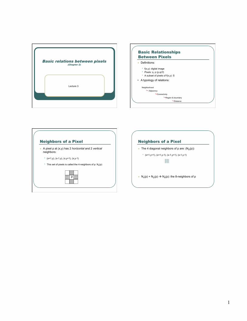
Neighbors of a Pixel   A pixel p at (x,y) has 2 horizontal and 2 vertical

neighbors:

•  (x+1,y), (x-1,y), (x,y+1), (x,y-1)

•  This set of pixels is called the 4-neighbors of p: N4(p)

p

Neighbors of a Pixel   The 4 diagonal neighbors of p are: (ND(p))

•  (x+1,y+1), (x+1,y-1), (x-1,y+1), (x-1,y-1)

  N4(p) + ND(p) N8(p): the 8-neighbors of p

p

Adjacent pixels

  Two pixels are adjacent if:

•  They are neighbors in some sense (e.g. N4(p), N8(p), …) •  Their gray levels satisfy a specified criterion of similarity V (e.g.

equality, …)

  V is the set of gray-level values used to define adjacency (e.g. V={1} for adjacency of pixels of value 1)

Adjacency (cont.)   p is adjacent to q if:

  We consider three types of adjacency:

•  4-adjacency: two pixels p and q with values from V are 4-adjacent if q is in the set N4(p)

•  8-adjacency: two pixels p and q with values from V are 8-adjacent if q is in the set N8(p)

€

q∈ N4 p( ),N8 p( ),...{ }f p( )∈ V

f q( )∈ V

⎧

⎨ ⎪

⎩ ⎪

2

Adjacency (cont.)   The third type of adjacency:

•  m-adjacency: p and q with values from V are m-adjacent if:

•  q is in N4(p)

or •  q is in ND(p) and the set N4(p)∩N4(q) has no pixels with values

from V

•  Mixed adjacency is a modification of 8-adjacency and is used to eliminate the multiple path connections that often arise when 8-adjacency is used.

Adjacency – An example

N4(p)∩N4(q)

Adjacency - An example N4(p)∩N4(q)

Subset Adjacency   Two image subsets S1 and S2 are adjacent if some pixel in S1 is

adjacent to some pixel in S2.

Paths   A path (curve) from pixel p with coordinates (x,y) to pixel q with

coordinates (s,t) is a sequence of distinct pixels:

•  Q : (x0,y0), (x1,y1), …, (xn,yn)

•  where (x0,y0)=(x,y), (xn,yn)=(s,t), and (xi,yi) is adjacent to (xi-1,yi-1), for 1≤i ≤n

•  n is the length of the path (|Q|).

  If (x0, y0) = (xn, yn), then Q is a closed path

  4-, 8-, and m-paths can be defined depending on the type of adjacency specified.

Connectivity   Connectivity between pixels is important for

establishing boundaries of objects and components of regions in an image

3

Connectivity   Two pixels (p∈S , q∈S) are connected in S if there

exists a path between them consisting entirely of pixels in S

  For any pixel p in S, the set of pixels in S that are connected to p is a connected component of S.

  If S has only one connected component then S is called a connected set.

Region & Boundary

  Let R be a subset of pixels:

• R is a region if R is a connected set.

•  Its boundary (border, contour) is the set of pixels in R that have at least one neighbor not in R

•  An edge can be the region boundary (in binary images)

Distance Measures

  For pixels p,q,z with coordinates (x,y), (s,t), (u,v), D is a distance function or metric if:

D(p,q) ≥ 0 (D(p,q)=0 iff p=q) D(p,q) = D(q,p) and D(p,z) ≤ D(p,q) + D(q,z)

Distance Measures

  Euclidean distance:

• De(p,q) = [(x-s)2 + (y-t)2]1/2

• Points (pixels) having a distance less than or equal to r from (x,y) are contained in a disk of radius r centered at (x,y).

Distance Measures

  D4 distance (city-block distance):

• D4(p,q) = |x-s| + |y-t| •  forms a diamond centered at (x,y) • e.g. pixels with D4≤2 from p

D4 = 1 are the 4-neighbors of p

Distance Measures

  D8 distance (chessboard distance):

• D8(p,q) = max(|x-s|,|y-t|) • Forms a square centered at p • e.g. pixels with D8≤2 from p

D8 = 1 are the 8-neighbors of p

4

Distance Measures   D4 and D8 distances between p and q are

independent of any paths that exist between the points because these distances involve only the coordinates of the points (regardless of whether a connected path exists between them).

  However, using m-adjacency the value of the distance (length of path) between two pixels depends on the values of the pixels along the path and those of their neighbors.

Distance Measures

  e.g. assume p, p2, p4 = 1 p1, p3 = can have either 0 or 1

If only connectivity of pixels valued 1 is allowed, and p1 and p3 are 0, the m-distance between p and p4 is 2.

If either p1 or p3 is 1, the distance is 3.

If both p1 and p3 are 1, the distance is 4 (p p1 p2 p3 p4)

Image Enhancements in the spatial domain: Intensity Transformations

(chapter 3)

(Lecture 3)

Image statistics   Consider an image f as a series of random samples, where each

pixel, f(x,y), is a sample at (x,y).

  The samples can be described by: •  The mean value (a measure of the overall brightness):

•  The standard deviation (a measure of the overall contrast):

•  Other summary statistics may also be used (min, max, median, …)

€

f =1

MNf x,y( )

N∑

M∑

€

σ =1

MNf x,y( ) − f ( )

2

N∑

M∑

Image Enhancement   Processing an image so that the result is more

suitable than the original image for a specific application. •  Problem oriented •  May be subjective

  There is no general theory of image enhancement

  Two primary categories (may be combined): •  Spatial domain methods •  frequency domain methods

Spatial Domain Methods

  Procedures that operate directly on the aggregate of pixels composing an image

 

  A neighborhood about (x,y) is defined by using a square (or rectangular) sub-image area centered at (x,y).

5

Spatial Domain Methods

  Mask processing or filtering:

•  when the values of f in a predefined neighborhood of (x,y) determine the value of g at (x,y).

•  Through the use of masks (or kernels, templates, or windows, or filters).

Spatial Domain Methods   When the neighborhood is 1 x 1 then g depends only on the value of f at

(x,y) and T becomes a gray-level transformation (or mapping) function (point operation):

s=T(r) , T:Z+→Z+

r and s are the gray levels of f(x,y) and g(x,y) at (x,y), where:

r denotes the pixel intensity before processing s denotes the pixel intensity after processing.

  “Point processing techniques” •  (e.g. contrast stretching, thresholding)

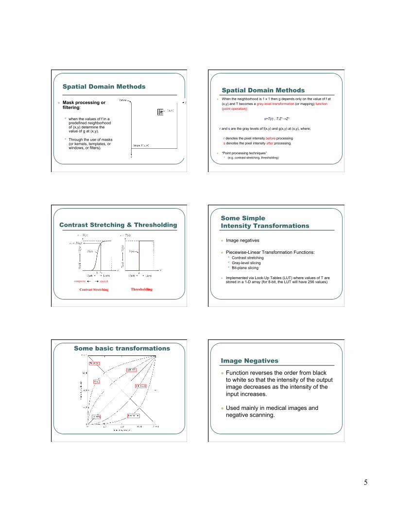
Contrast Stretching Thresholding

Contrast Stretching & Thresholding Some Simple Intensity Transformations

  Image negatives

  Piecewise-Linear Transformation Functions: •  Contrast stretching •  Gray-level slicing •  Bit-plane slicing

  Implemented via Look-Up Tables (LUT) where values of T are stored in a 1-D array (for 8-bit, the LUT will have 256 values)

Some basic transformations

Image Negatives

  Function reverses the order from black to white so that the intensity of the output image decreases as the intensity of the input increases.

  Used mainly in medical images and negative scanning.

6

Negative of an image   The negative is obtained by using the following

transformation function s=T(r):

[0,L-1] the range of gray levels S= L-1-r

Negative - example Aerial image The negative

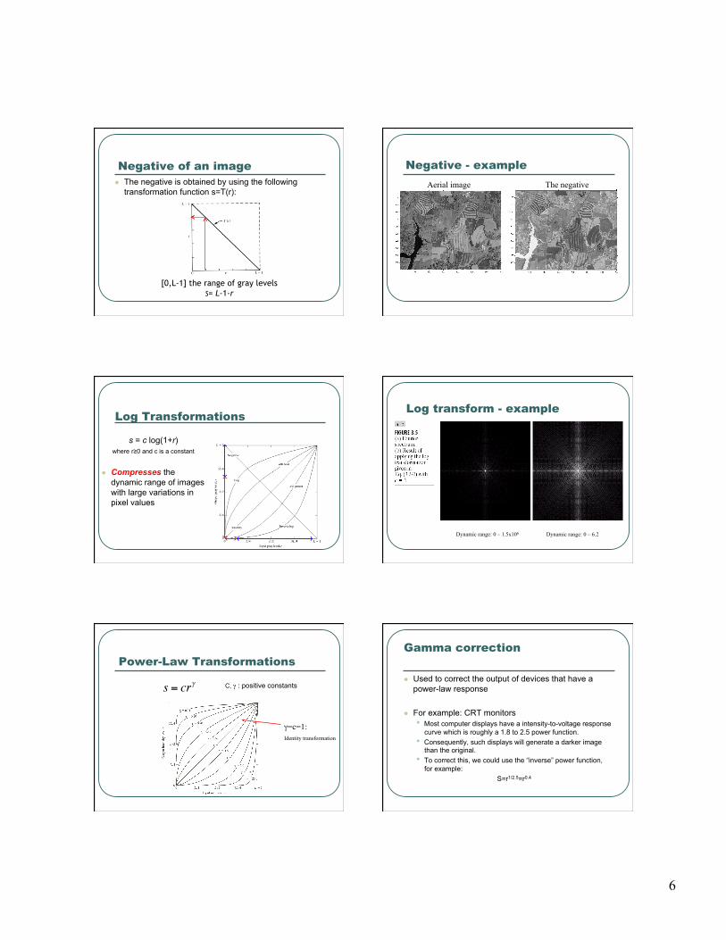
Log Transformations

s = c log(1+r) where r≥0 and c is a constant

  Compresses the dynamic range of images with large variations in pixel values

Dynamic range: 0 – 1.5x106 Dynamic range: 0 – 6.2

Log transform - example

Power-Law Transformations

C, γ : positive constants

γ=c=1: Identity transformation

Gamma correction

  Used to correct the output of devices that have a power-law response

  For example: CRT monitors •  Most computer displays have a intensity-to-voltage response

curve which is roughly a 1.8 to 2.5 power function. •  Consequently, such displays will generate a darker image

than the original. •  To correct this, we could use the “inverse” power function,

for example: S=r1/2.5=r0.4

7

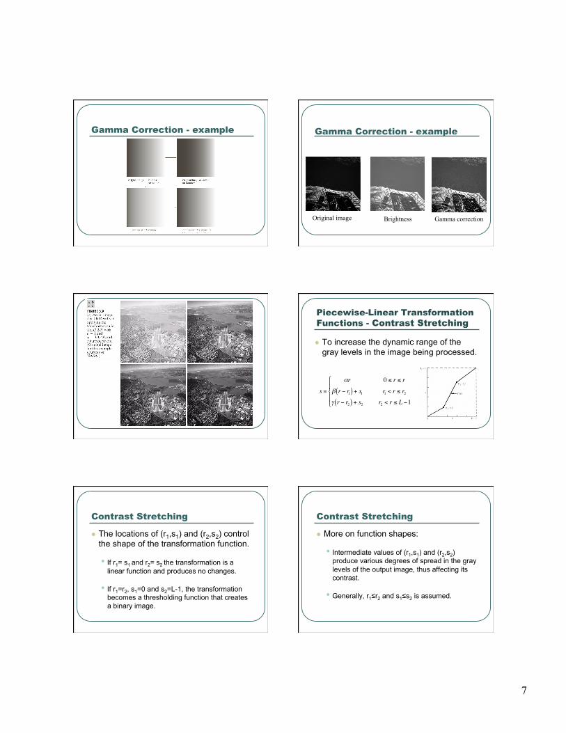
Gamma Correction - example Gamma Correction - example

Original image Brightness Gamma correction

Piecewise-Linear Transformation Functions - Contrast Stretching

  To increase the dynamic range of the gray levels in the image being processed.

€

s =

αr 0 ≤ r ≤ r

β r − r1( ) + s1 r1 < r ≤ r2γ r − r2( ) + s2 r2 < r ≤ L −1

⎧

⎨ ⎪

⎩ ⎪

Contrast Stretching

  The locations of (r1,s1) and (r2,s2) control the shape of the transformation function.

•  If r1= s1 and r2= s2 the transformation is a linear function and produces no changes.

•  If r1=r2, s1=0 and s2=L-1, the transformation becomes a thresholding function that creates a binary image.

Contrast Stretching

  More on function shapes:

•  Intermediate values of (r1,s1) and (r2,s2) produce various degrees of spread in the gray levels of the output image, thus affecting its contrast.

• Generally, r1≤r2 and s1≤s2 is assumed.

8

Gray-Level Slicing

  To highlight a specific range of gray levels in an image (e.g. to enhance certain features).

One way is to display a high value for all gray levels in the range of interest and a low value for all other gray levels (binary image).

Gray-Level Slicing

• The second approach is to brighten the desired range of gray levels but preserve the background and gray-level tonalities in the image:

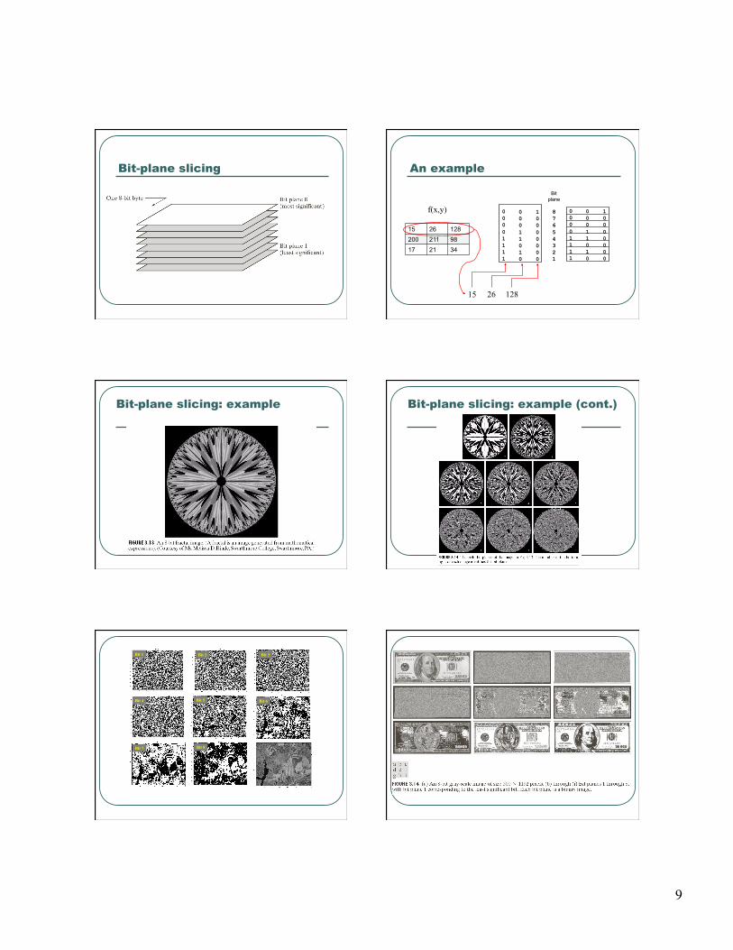
Bit-Plane Slicing   Analyzing the contribution made to the total image

appearance by specific bits.

•  i.e. Assuming that each pixel is represented by 8 bits, the image is composed of 8 1-bit planes.

•  Plane 0 contains the least significant bit and plane 7 contains the most significant bit.

•  Bit-plane slicing is useful for image compression

Bit-Plane Slicing

• Usually, only the higher order bits (top four) contain visually significant data. The other bit planes contribute the more subtle details.

• Plane 7 corresponds exactly with an image thresholded at gray level 128.

9

Bit-plane slicing An example

15 26 128

f(x,y)

15 26 128 200 211 98 17 21 34

Bit-plane slicing: example Bit-plane slicing: example (cont.)

Bit 1 Bit 2 Bit 3

Bit 4 Bit 5 Bit 6

Bit 7 Bit 8

10

Bit-plane slicing: example