Better Lucky Than Rich? Welfare Analysis of Automobile License

Allocations in Beijing and Shanghai∗

Shanjun Li†

March 2014

Abstract

Economists often favor market-based mechanisms over non-market based mechanisms

to allocate scarce public resources on grounds of economic efficiency and revenue gener-

ation. When the usage of the resources in question generates type-dependent negative

externalities, the welfare comparison can become ambiguous. Both types of allocation

mechanisms are being implemented in China’s major cities to distribute limited vehi-

cle licenses as a measure to combat worsening traffic congestion and urban pollution.

While Beijing employs non-transferable lotteries, Shanghai uses an auction system.

This study empirically quantifies the welfare consequences of the two allocation mech-

anisms by estimating a random coefficients discrete choice model of vehicle demand

to recover consumers’ willingness to pay for a license. Rather than relying on the

maintained exogeneity assumption on product attributes in the literature, we employ

a novel strategy by taking advantage of a control group as well as information from

household surveys to identify structural parameters. Our analysis finds that although

Beijing’s lottery system has a large advantage in reducing automobile externalities over

auction, the advantage is offset by the significant allocative cost from misallocation.

The lottery system foregone nearly 36 billion RMB ($6 billion) in social welfare in 2012

and a uniform price auction would have generated 21 billion RMB to Beijing municipal

government, more than covering all the subsidies to the local public transit system.

Keywords: Auction, Lottery, Random Coefficients Utility Model, Resource Allocation

JEL classification: L9, Q58, R48

∗I thank Antonio Bento, Sebastien Houde, Sabrina Howell, Sarah Jacobson, Matthew Kahn, NehaKhanna, Benjamin Leard, Joshua Linn, Yimin Liu, Stuart Rosenthal, Emily Wang, Catherine Wolfram,Jun Yang and seminar participants at Binghamton University, Ford Motor Company, NBER, Shanghai Uni-versity of Finance and Economics, University of Massachusetts - Amherst, and University of Sao Paulo forhelpful suggestions. Financial support from the Lehman fund at Cornell University is acknowledged. Allerrors are my own.†Assistant Professor, Dyson School of Applied Economics and Management, Cornell University, 405

Warren Hall, Ithaca, NY 14853. Email: SL2448@cornell.edu. Phone: (607)255-1832.

1 Introduction

Market-based mechanisms (e.g., auction) have often been advocated for allocating scarce

public resources on grounds of economic efficiency and revenue generation, as opposed to non-

market based mechanisms (e.g., lottery). Both have been used widely in practice, often for

different types of resources. For example, auctions are routinely used to sell mineral rights,

timber, and radio spectrum while lotteries are employed in distributing hunting licenses,

charter school admissions, and jury duty.1 Market-based mechanisms have the potential

to achieve efficiency by using price signals to distribute the scarce resource to those with

the highest willingness to pay (WTP), whereas lotteries with no-transferability can lead

to misallocation and unrealized welfare gain. However, when the usage of the resources

generates negative externalities that are increasing in WTP, the welfare comparison between

the two mechanisms can become ambiguous. In this case, the social benefit (consumer welfare

net of externalities), the basis for measuring social welfare, diverges from and may even be

decreasing with WTP, the basis for resource allocation under the market-based mechanisms.

The resource in question here is a license or permit to register a vehicle. Major cities in

China have been experiencing the world’s worst traffic congestion and air pollution as a result

of rapid economic growth as well as vehicle ownership outpacing transport infrastructure

and environmental regulation.2 Beijing, the second largest city in China, has been routinely

ranked as one of the cities with worst traffic conditions in the world, with the average traffic

speed during peak hours below 15 miles per hour. The daily concentration of PM2.5, a key

measure of air quality, frequently reaches over 10 times of the daily health limit recommended

by the World Health Organization (WHO). To ease gridlock and improve air quality, Beijing

municipal government introduced a quota system for vehicle licenses in 2011 in order to

limit the growth of vehicle ownership. About 20,000 new licenses are distributed each month

through non-transferable lotteries. Winning the lottery has become increasingly difficult:

the odds decreased from 1:10 in January 2011 to 1:100 by the end of 2013.

Shanghai, the largest city in China, also has a vehicle license quota system but its license

allocation is through an auction system instead of lotteries. In fact, an auction system has

1The Federal Communications Commission used both administrative process and lotteries to allocateradio spectrum in the early years, both of which led to wide discontent due to long delays. The FCC finallyadopted auctions in 1994 after many decades of persistent arguments by economists. The first auction yieldedten times of revenue predicted by the Congressional Budget Office (Cramton 2002).

2New automobile sales in China grew from 2.4 million units in 2001 to 19.30 million in 2012, surpassingthe U.S. to become the largest market in 2009. Zheng and Kahn (2013) offer a comprehensive review onChina’s urban pollution challenges and government policies to deal with them.

1

been in place since 1986 but the goal of reducing vehicle ownership did not emerge until

much recently. The current form of multi-unit, discriminatory and dynamic auction started

in 2008 and auctions are held monthly online to distribute about 10,000 licenses. In 2012,

the auction system generated over 6.7 billion RMB (about $1 billion) to Shanghai municipal

government. The average bid for a license reached over 92,000 RMB in March 2013, higher

than the price of many entry-level vehicle models.

The main objective of this study is to empirically quantify the welfare consequences of the

two allocation mechanisms in distributing vehicle licenses taking into account both allocation

efficiency and externalities associated with vehicle usage. This is an important question for

at least two reasons. First, traffic congestion and air pollution impose major costs to the

society, especially in emerging markets (Parry et al. 2007). Creutzig and He (2008) estimate

that the external costs from automobile usage in Beijing amount to over 7.5% of its GDP.

Under the endorsement of China’s Ministry of Environmental Protection, many large cities

in China are adopting license quota systems and some version of allocation mechanisms.3

However, the impacts and welfare consequences of these policies are unknown.

Second, there is theoretical ambiguity a priori in welfare comparison between the two

mechanisms because the usage of license (registering and ultimately driving a vehicle) is as-

sociated with negative externalities such as congestion and pollution. These type-dependent

externalities are likely to be increasing in consumers’ WTP for a license in that consumers

with high WPT tend to have high income, buy less fuel-efficient vehicles and drive more.

Whether the lottery or the auction system leads to higher social welfare depends critically

on the level of consumer heterogeneity in WTP and its relationship with automobile ex-

ternalities. Therefore, the efficiency comparison and the magnitude of welfare impacts are

ultimately empirical questions.

Since licenses are allocated through lotteries and trade is not allowed in Beijing, we do

not observe consumers’ WTP. In Shanghai, licenses are auctioned in a non-standard format

and the bids may not reflect value as shown in an experimental study by Liao and Holt

(2013). To recover consumers’ WTP for a license, we estimate a random coefficients discrete

choice model of vehicle demand that takes into account consumer preference heterogene-

ity and unobserved product attributes developed by Berry, Levinsohn, and Pakes (1995)

(henceforth BLP). Similar to Petrin (2002), our estimation strategy employs both aggregate

market-level data and information from household surveys to form moment conditions. From

3Cities of Guiyang and Guangzhou adopted license lotteries in July 2011 and August 2012, respectively.Tianjin and Hangzhou started to implement a hybrid system in January and March 2014.

2

household surveys on new vehicle buyers, we obtain the share of buyers among different in-

come groups. We used them to form (micro-) moment conditions and they are critical in

identifying consumer preference heterogeneity.

An important departure in our identification strategy from the literature is that we

do not rely on the maintained exogeneity assumption that unobserved product attributes

are uncorrelated with observed product attributes. Rather, we employ the common trend

assumption used in the difference-in-differences (DID) framework for impact evaluation.

This is possible because our market-level data include data for four cities: Beijing, Nanjing,

Shanghai, and Tianjin. Nanjing and Tianjin are two large cities next to Shanghai and

Tianjin, respectively. They did not have the license quota system during the data period

and as we show through graphs and regressions, the automobile markets in these two cities

exhibit similar trends to Beijing and Shanghai in the absence of the policies.

Several important findings emerge from our analysis. First, both policies in Beijing and

Shanghai significantly limited new vehicles sales: the lottery system in Beijing reduced new

vehicle sales by over one million in 2011 and 2012 while the Shanghai auction reduced sales

by about 1.4 million from 2008 to 2012. These reductions are substantial and a reflection of

the stringency of the quota system. Second, while Beijing’s lottery system has a non-trivial

advantage (7 billion RMB) over an auction system in reducing automobile externalities, its

allocative cost due to misallocation is nearly 43 billion RMB in 2012, implying a welfare loss

of nearly 36 billion RMB. The significant allocative cost from the lottery system is driven

by the large consumer heterogeneity in WTP for licenses. Third, a uniform price auction

would have generated 21 billion revenue to Beijing municipal government in 2012, more than

enough to cover all its subsidies to the local public transit system. Fourth, based on a range

of plausible assumptions, the optimal level of quota in Beijing is lower than the existing level

and further reducing the quota would increase net social welfare.

This study contributes to the literature in the following four aspects. First, although

theoretical literature on allocation mechanisms are abundant, there are very few empirical

studies on quantifying welfare outcomes of different mechanisms. Glaeser and Luttmer (2003)

study housing market rationing under the rent control in New York city and provide evidence

of significant misallocation of houses, without explicitly estimating the allocative cost. Davis

and Kilian (2011) find significant allocative costs from misallocation under the price ceiling

in the U.S. residential market for natural gas. In the context of a quantity regulation, this

paper empirically examine allocative outcomes by exploring a rare opportunity where both

market-based and non-market mechanisms are used for the same type of resources.

3

Second, as we discussed above, in the presence of type-dependent externalities that is

increasing in WTP, the efficiency comparison between the lottery and auction systems could

be ambiguous due to the fact that externalities introduce a wedge between net social benefit,

the basis for measuring social welfare, and the private benefit, the basis of resource allocation

under auction. The implication of type-dependent externalities on optimal allocation mech-

anisms has been examined in several theoretical studies in the context of firm competition.4

Our analysis empirically highlights type-dependent externalities in the context of consumer

goods and showcases the advantage of the lottery system in reducing externalities.

Third, our analysis adds to the emerging literature on China’s environmental and energy

policies. China is by far the largest emitter of greenhouse gases, accounting for nearly 30

percent of world emissions in 2012. It is the largest energy consumer and is also the top

importer of crude oil in the world. China’s domestic policies could have global impacts but

our understanding on the impacts of these policies is very limited.5

Fourth, our study offers a novel identification strategy in structural demand estimation

by employing the common trend assumption used in DID analysis. This alleviates the need

to rely on the maintained assumption in the literature which is often deemed strong since

vehicles attributes are likely to be jointly determined in the design process. Our empirical

strategy to recover consumers’ WTP for licenses combines both the structural demand model

and the DID method. The structural demand model allows consumer heterogeneity that is

critical for the welfare analysis while the DID framework provides us an alternative method

to identify structural parameters while at the same time offering a benchmark for examining

the validity of the predictions from the structural model.

Before we proceed, it is perhaps helpful to further clarify the scope of our welfare analysis.

First, our analysis focuses on the welfare consequences of different allocation mechanisms

within the policy framework of a quota system. Automobile usage generates multiple types of

externalities including congestion, air pollution, traffic accidents and noise. A vehicle license

quota system in theory is not the first-best instrument to internalize these externalities since

4Brocas (2013) analyzes optimal auction design with type-dependent negative externalities in the contextof multiple firms competing for the acquisition of a technology license or a procurement contract. The winnerinduces a negative externality on the loser since the winner will have a competitive advantage over the loserin downstream competition.

5Various federal and local policies are being adopted in China to address urban congestion and airpollution including fuel economy standards, emission standards, gasoline tax, and driving restrictions. Chenet al. (2011) study the environmental impacts of measures such as driving restriction and plant closure bythe Beijing government to clear up the air before the 2008 Olympic Games. Xiao and Heng (2013) evaluateand compare the effects of favorable consumption tax treatment for small vehicles and the gasoline tax.

4

it does not directly address the source of externalities, i.e., driving.6 Second, our analysis

focuses welfare impacts in the short run. The allocation of vehicle licenses are likely to have

impacts on household location, job decision and schooling choices, all of which could have

important welfare implications in the long term. Although part of these welfare impacts such

as the desire to live in a large apartment outside of the city center and hence the need to have

a vehicle are captured by the WTP that we estimate, we are not investigating the policy

impacts in these dimensions. The broader welfare comparisons between the quota system

with other potentially more efficient policy instruments such as congestion pricing and fuel

taxes as well as long-run analysis will necessitate additional information and modeling efforts.

We leave them for future research.

2 Allocation Mechanisms and Externalities

The purpose of this section is to offer an illustration on the welfare comparison between

lottery and auction systems in the presence of type-dependent negative externalities. In

allocating scarce public resources, governments or resource managers have relied on both

market-based mechanisms and non-market based mechanisms often for different types of

goods. Market-based mechanisms such as a well-designed auction can allocate the resource to

those with the highest value and hence achieve efficiency while non-market based mechanisms

such as an administration process or lottery do not. It is argued that non-market based

mechanisms such as a lottery are chosen often out of concern of fairness or for political

convenience (Taylor et al. 2003).

However, when the usage of resources generates market failures such as externalities,

market-based mechanisms such as an auction may not yield efficient allocation because the

private value and the social benefit diverge.7 We illustrate this point within the context of

allocating vehicle licenses using lotteries and auctions. Consider the following environment:

(1) there are Q licenses to be allocated; (2) there are N(N > Q) agents, each demanding

at most one license; (3) each agent i has a private value (or WTP) Vi and the value is

6In the first-best world, multiple instruments should be used to correct for these externalities. Forexample, real-time congestion pricing is the first-best instrument to deal with congestion externality while fueltaxes is the first-best instrument to internalize the externality from CO2 emissions and other pollutants thatare proportional to fuel use. Nevertheless, these policy instruments would require different administrativecosts. The quota system has become a popular policy option among local policy makers perhaps for its loweradministrative costs or due to inertia from traditional command-and-control regulatory approach.

7The usage of licenses by firms may have implications on market power. This has been discussed in thecontext of spectrum auctions where different collection of winners may subsequently lead to different marketstructure (Cramton 2002).

5

drawn from a known i.i.d. distribution with a support of [0, V ]; (4) the usage of the license

imposes an external cost of Ei, which is increasing in Vi. The fourth assumption of type-

dependent externalities is a key departure from a standard model of resource allocation. As

we document below, consumers with high WTP for a license tend to have higher income. On

average, they drive larger and less fuel-efficient vehicles and they drive more relative to those

with a low WTP. So the usage of licenses by those with a higher WTP is likely to generate

larger external costs. Our estimates below show that neither the magnitude of external costs

nor the difference in external costs across households is trivial. That is, the discussion below

does have empirical relevance in our context.

We compare two allocation mechanisms: a non-transferable lottery where all agents can

participate and have an equal chance of winning (random allocation); and a uniform price

auction where the Q highest bidders each gets one license and pays a price equal to the

highest rejected bid. Harris and Raviv (1981) show that each agent bids her value in this

auction and therefore the licenses will be allocated to the Q agents with the highest value.

We use the uniform price auction for exposition and the point is not lost with other types

of auctions such as discriminatory auctions that can achieve the same allocation outcome.

We start with a simple case of allocation mechanisms with constant external costs from

the usage of the license and ultimately automobiles as depicted in the top panel of Figure 1.

Line Q(p) is the (smoothed) WTP schedule. Line EC is the external cost for the agents with

the corresponding WTP and it is constant in this case. Assuming the quota Q is lower than

the optimal cap Q∗, the area BCD is the conventional deadweight loss (DWL) from quantity

constraint. Total consumer surplus from the auction system is given by the area ABQO but

the lottery system can only realize Q/Q1 of these surplus from the random allocation, which

is given by AQO. Therefore, the allocative cost, i.e., welfare loss from misallocation, of the

lottery system is ABQ, which could even be larger than the DWL from quantity constraint.

The empirical importance of allocative cost from random allocation is highlighted in Davis

and Kilian (2011) in the context of price ceiling in the U.S. residential natural gas market.

The middle panel in Figure 1 shows a case where the external costs are positively corre-

lated with WTP. As in the top panel, BCD is the DWL from quantity constraint and ABQ

is the allocative cost from the lottery system. However, the presence of type-dependent ex-

ternal costs implies that the lottery system leads to a reduction in external costs depicted by

EDF, offsetting part of the allocative cost. The net welfare loss from lottery (versus auction)

is given by the area ABQ - EDF, which is positive in this case. The advantage in reducing

externalities from the lottery system is dominated by the welfare loss from misallocation,

6

implying that the auction system still produces a better welfare outcome.

The welfare comparison between the two systems is reversed in the bottom panel where

the external costs are “strongly” increasing in WTP. To ease exposition, we assume that

the quota Q is at the intersection of the WTP schedule and the corresponding external

cost curve. In this case, the reduction in external costs from the lottery given by EBQO

dominates the allocative cost given by ABQ. Since agents with the highest private value

generates the smallest social value, the auction will allocate the licenses to the wrong hands

from the efficiency perspective. This result is driven by the fact that the wedge introduced

by the external costs between the private value and the social value leads to a negative

correlation between the two. Note that the external cost line does not have to surpass the

WTP schedule as shown in the graph to make the point. The result could still hold if the

EC line is below the WTP schedule but is steeper.

Which of the two scenarios is playing out in reality depends on the WTP schedule as well

as its relationship with the external cost curve. Although one can get a good sense on the

external costs from driving from different households based on household survey data, the

WTP schedule is not readily available. The empirical goal is to develop a method to estimate

the WTP schedule and conduct welfare comparison taking into account the external costs.

3 Policy and Data Description

In this section, we first describe the background for the quota systems. We then discuss the

lottery and auction policies in Beijing and Shanghai and present our data thereafter.

3.1 Background

During the past three decades, China has embarked on an extraordinary journey of economic

growth with its GDP growing at about 10 percent a year. As household income grows, luxury

good consumption such as automobiles started to pick up dramatically around the turn of

the century. The annual sales of new passenger vehicles increased from 2.4 million units in

2001 to over 19 million units in 2012 as depicted in Appendix Figure 1, surpassing the U.S.

to become the largest market in 2009. Large cities in China are ahead of the curve in both

economic growth and vehicle ownership. Beijing with about seven million households has

gone from a city on bikes to a city on cars during this period: the stock of passenger vehicles

increased from 1.6 million units to nearly 5 million units as shown in Appendix Figure 1.8

8Among the 5 million vehicles, about 4 million are owned by households. The household vehicle ownershiprate is 0.58 in Beijing, comparing to 0.46 in New York city and 1.16 in the U.S. from 2010 U.S. Census.

7

The rapid growth in vehicle ownership leads to serious traffic congestion, despite signifi-

cant efforts in expanding roads and public transit systems and a whole range of other traffic

management policies such as driving restrictions and reducing public transit fares. The city

is now often ranked routinely as one of the worst cities in traffic conditions. The traffic

speed on arterial roads within the 5th ring road during morning peak hours (7:00-9:00) on

work days averaged 14.7 miles/hour (MPH) in 2011, reduced from 22.8 MPH in 2005. The

average speed was 13.4 MPH during afternoon peak hours (17:00-19:00) in 2011, compared

with 20.2MPH in 2005. During the same period, air quality has worsened dramatically and

the air quality index is frequently above the hazardous level defined by the U.S. EPA which

recommends that everyone should avoid all outdoor physical activities.9

Shanghai with 8.5 million households has slightly better traffic conditions that are on

par with those in Los Angeles. The traffic speed on arterial roads averages 21.2MPH and

22.3MPH during morning and evening peak, respectively. As shown in the bottom panel

of Appendix Figure 1, the total number of vehicles in Shanghai is less than half of that

in Beijing, despite having more households and higher average household income. This is

largely due to vehicle purchase restrictions put in place before vehicle ownership took off as

we discuss below. The air quality in Beijing is consistently worse than Shanghai due to more

vehicles, worse traffic, and winter heating coupled with unfavorable topography. In a ranking

of air quality among 28 major cities on the east coast, Beijing ranked at the bottom with

an annual average PM10 concentration of 121 micrograms per cubic meter while Shanghai

ranked at 8th with an average PM10 concentration of 79 in 2010, still significantly higher

than the WHO’s health limit.

3.2 Policy Description

To address traffic congestion and air pollution, Beijing municipal government announced the

policy of capping new vehicle licenses which are necessary to register a vehicle, on December

23, 2010. Since January 2011, lotteries have been used to allocate about 20,000 licenses each

month. A license is needed for first-time buyers, and those who purchase an old vehicle,

accept a gifted vehicle, or transfer out-of-state registration to Beijing. Vehicle owners who

9The average daily concentration of PM2.5 frequently reaches over 250 micrograms per cube meter,compared to the recommended daily level of 20 by WHO. The city may have seen the worst air pollution sofar in Jan. 2013. During the 24-hour period from 10am on Jan. 12th, 18 of the 24 hourly PM2.5 reading inthe U.S. Embassy were beyond 500 micrograms per cube meter, with the highest record of 866. Accordingto Beijing Environmental Protection Bureau, automobiles are the largest source of PM2.5, accounting for 22percent in the whole city and about one third in the urban core. The second largest source of PM2.5 is coalburning (17 percent) followed by construction site dusts (16 percent) in 2012.

8

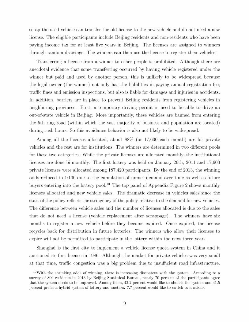
scrap the used vehicle can transfer the old license to the new vehicle and do not need a new

license. The eligible participants include Beijing residents and non-residents who have been

paying income tax for at least five years in Beijing. The licenses are assigned to winners

through random drawings. The winners can then use the license to register their vehicles.

Transferring a license from a winner to other people is prohibited. Although there are

anecdotal evidence that some transferring occurred by having vehicle registered under the

winner but paid and used by another person, this is unlikely to be widespread because

the legal owner (the winner) not only has the liabilities in paying annual registration fee,

traffic fines and emission inspections, but also is liable for damages and injuries in accidents.

In addition, barriers are in place to prevent Beijing residents from registering vehicles in

neighboring provinces. First, a temporary driving permit is need to be able to drive an

out-of-state vehicle in Beijing. More importantly, these vehicles are banned from entering

the 5th ring road (within which the vast majority of business and population are located)

during rush hours. So this avoidance behavior is also not likely to be widespread.

Among all the licenses allocated, about 88% (or 17,600 each month) are for private

vehicles and the rest are for institutions. The winners are determined in two different pools

for these two categories. While the private licenses are allocated monthly, the institutional

licenses are done bi-monthly. The first lottery was held on January 26th, 2011 and 17,600

private licenses were allocated among 187,420 participants. By the end of 2013, the winning

odds reduced to 1:100 due to the cumulation of unmet demand over time as well as future

buyers entering into the lottery pool.10 The top panel of Appendix Figure 2 shows monthly

licenses allocated and new vehicle sales. The dramatic decrease in vehicles sales since the

start of the policy reflects the stringency of the policy relative to the demand for new vehicles.

The difference between vehicle sales and the number of licenses allocated is due to the sales

that do not need a license (vehicle replacement after scrappage). The winners have six

months to register a new vehicle before they become expired. Once expired, the license

recycles back for distribution in future lotteries. The winners who allow their licenses to

expire will not be permitted to participate in the lottery within the next three years.

Shanghai is the first city to implement a vehicle license quota system in China and it

auctioned its first license in 1986. Although the market for private vehicles was very small

at that time, traffic congestion was a big problem due to insufficient road infrastructure.

10With the shrinking odds of winning, there is increasing discontent with the system. According to asurvey of 800 residents in 2013 by Beijing Statistical Bureau, nearly 70 percent of the participants agreethat the system needs to be improved. Among them, 42.2 percent would like to abolish the system and 41.5percent prefer a hybrid system of lottery and auction. 7.7 percent would like to switch to auctions.

9

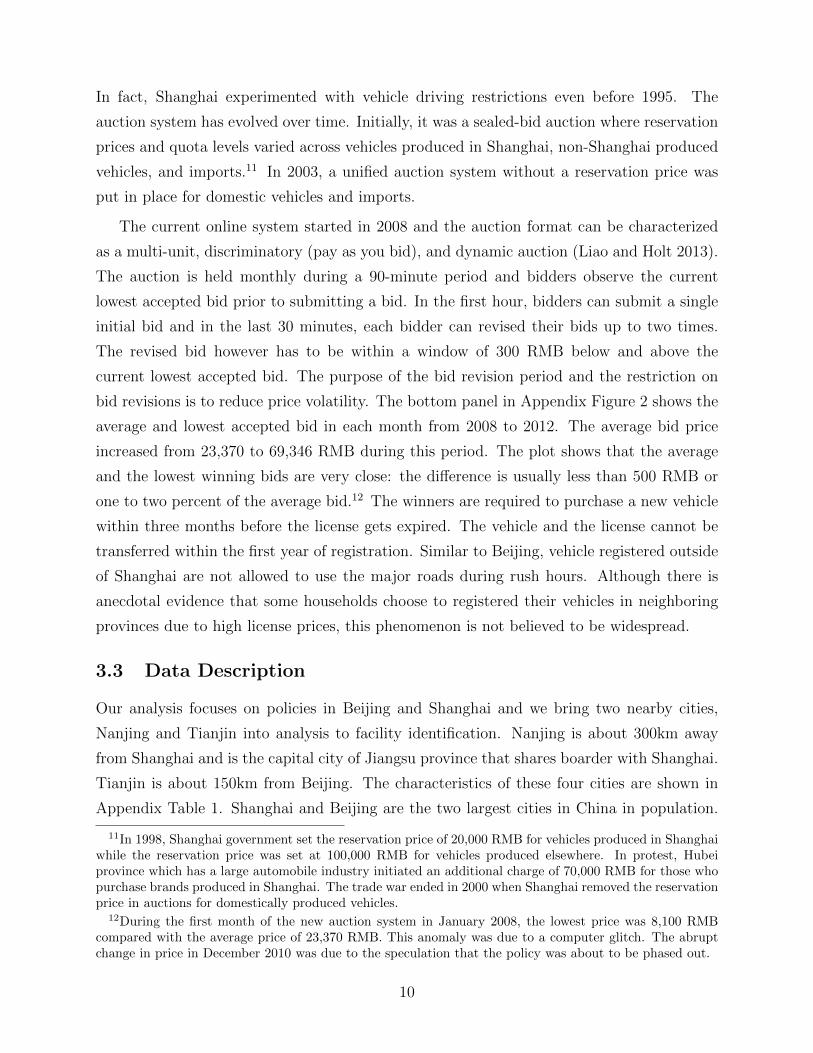
In fact, Shanghai experimented with vehicle driving restrictions even before 1995. The

auction system has evolved over time. Initially, it was a sealed-bid auction where reservation

prices and quota levels varied across vehicles produced in Shanghai, non-Shanghai produced

vehicles, and imports.11 In 2003, a unified auction system without a reservation price was

put in place for domestic vehicles and imports.

The current online system started in 2008 and the auction format can be characterized

as a multi-unit, discriminatory (pay as you bid), and dynamic auction (Liao and Holt 2013).

The auction is held monthly during a 90-minute period and bidders observe the current

lowest accepted bid prior to submitting a bid. In the first hour, bidders can submit a single

initial bid and in the last 30 minutes, each bidder can revised their bids up to two times.

The revised bid however has to be within a window of 300 RMB below and above the

current lowest accepted bid. The purpose of the bid revision period and the restriction on

bid revisions is to reduce price volatility. The bottom panel in Appendix Figure 2 shows the

average and lowest accepted bid in each month from 2008 to 2012. The average bid price

increased from 23,370 to 69,346 RMB during this period. The plot shows that the average

and the lowest winning bids are very close: the difference is usually less than 500 RMB or

one to two percent of the average bid.12 The winners are required to purchase a new vehicle

within three months before the license gets expired. The vehicle and the license cannot be

transferred within the first year of registration. Similar to Beijing, vehicle registered outside

of Shanghai are not allowed to use the major roads during rush hours. Although there is

anecdotal evidence that some households choose to registered their vehicles in neighboring

provinces due to high license prices, this phenomenon is not believed to be widespread.

3.3 Data Description

Our analysis focuses on policies in Beijing and Shanghai and we bring two nearby cities,

Nanjing and Tianjin into analysis to facility identification. Nanjing is about 300km away

from Shanghai and is the capital city of Jiangsu province that shares boarder with Shanghai.

Tianjin is about 150km from Beijing. The characteristics of these four cities are shown in

Appendix Table 1. Shanghai and Beijing are the two largest cities in China in population.

11In 1998, Shanghai government set the reservation price of 20,000 RMB for vehicles produced in Shanghaiwhile the reservation price was set at 100,000 RMB for vehicles produced elsewhere. In protest, Hubeiprovince which has a large automobile industry initiated an additional charge of 70,000 RMB for those whopurchase brands produced in Shanghai. The trade war ended in 2000 when Shanghai removed the reservationprice in auctions for domestically produced vehicles.

12During the first month of the new auction system in January 2008, the lowest price was 8,100 RMBcompared with the average price of 23,370 RMB. This anomaly was due to a computer glitch. The abruptchange in price in December 2010 was due to the speculation that the policy was about to be phased out.

10

Tianjin is the sixth and Nanjing is the 11th.13 Shanghai has the highest average household

income while Tianjin has the lowest. Appendix Table 1 shows that Beijing has the smallest

increase in average nominal income of 42% during the 5-year period while Shanghai has the

largest increase of 57%, with the inflation being 13.7% during this period.

We rely on four main data sets together with a variety of auxiliary data for our analysis.

The first main data set contains monthly vehicle sales by model (vintage-nameplate) in each

city from 2008 to 2012. There are 21,228 observations with 1,769 distinct models. Figure

2 plots monthly sales (in log) in each city and displays two important features. First, sales

in all four cities grew over time and tracked each other well before 2011 and the trend is

more consistent across Beijing, Nanjing and Tianjin, reflecting the fact that Shanghai has

an auction policy in place throughout the data period. Second, there was strong seasonality

which is largely driven by holidays. The sales in December 2010 went up dramatically

in all cities but then dropped significantly in February 2011. This is due to the fact that

Chinese New Year was in February 3rd in 2011.14 Third, the sales increase in December 2011

appeared to be stronger in Beijing than in other cities. This is due to the anticipation and

more importantly the fact that the quota policy was announced in December 23, 2010. Very

little if any discussion on the policy was made public before the announcement. However,

once the policy was announced, many who planned to buy a vehicle in the next few months

moved their purchase forward into the last week of December. In the main specification of

our analysis, we remove the last two months in 2010 and the first two months in 2011 in

Beijing to deal with the anticipation and more importantly announcement effects.

The second data set contains vehicle characteristics of each model in the sales data. These

characteristics include price, fuel economy (liters/100km), vehicle size, engine size, vehicle

type, and vehicle segment. The summary statistics are presented in Table 1. Vehicle prices

are computed based on the Manufacturer Suggested Retail Prices (MSRPs) and the sales

tax. MSRPs are set by manufacturers and are generally constant across locations and within

a model year. There could be potential pitfalls in using MSRPs when they are different from

the transaction prices due to promotions. Different from the promotion-heavy environment

in the U.S., China’s auto market has infrequent promotions from manufactures or dealers

and retail prices are often very close to or the same as MSRPs, a phenomenon commonly

seen for luxury products in China. Our analysis uses MSRPs with the implicit assumption

13Beijing, Shanghai and Tianjin are three of the four province-level cities. They are at the same level ofadministrative subdivision as provinces and are right below the central government.

14During the holiday season that starts from at least one week before the Chinese New Year and ends twoweeks after, people are occupied with visiting families and friends. Big-item purchases such as buying a cartend to occur before the holiday season.

11

that the allocation mechanisms in Shanghai and Beijing are not likely to affect firms price-

setting behavior or local dealer incentives. This assumption should not be a driving factor in

our results given the small market shares of these two cities and the marketing environment

for automobiles in China.15 The sales tax is normally set at 10% but was reduced to 5 and

7.5 percent for vehicles with engine displacement no more than 1.6 liter in 2009 and 2010,

respectively. The average price of a vehicle is over 300,000 RMB and the medium price is

over 190,000, both significantly higher than the average household income these cities.

The third data set is income distributions by city by year. China’s National Bureau of

Statistics conducts census every 10 years but the income data at the household level are

not publicly available. Instead, we obtain the average income by income quantiles in each

city in each year from the statistical yearbooks of each city. We construct household income

distribution based on these aggregate information together with Chinese Household Income

Survey (2002), a national representative survey, conducted by researchers at the University

of Michigan. We adjust the income in the household survey (14,971 obs.) proportionally

and separately for each of the quantiles so that the interpolated income distributions in a

given year are consistent with the annual income statistics from the yearbooks.

The fourth set of data contains aggregate information from an annual national repre-

sentative household survey among new vehicle buyers from Ford Motor Company. We were

provided household shares by four income groups among new vehicles buyers in each city in

each year. Appendix Table 2 presents these shares along with the shares of different income

group among all households, which are constructed based on the income distributions from

each city. The table shows that high income groups account for a disproportionally large

share of vehicle buyers. While the highest income group (annual household income over

144,000) accounts for 3.85% of all households in 2012 in Beijing, this group accounts for

more than 20% of new vehicle buyers. These information will be used to form additional

moment conditions that are crucial to identify consumer preference parameters.

4 Empirical Model of Vehicle Demand

In order to conduct welfare analysis, we need to recover consumers’ WTP for a license. We do

not observe license prices in Beijing since the licenses are allocated through lottery for free.

In Shanghai, although we observe average bids, they are unlikely to represent consumers’

15Li et al. (2013) offer a detailed discussion on the industry and examine various factors underlying pricechanges over time. MSRPs already include two types of taxes: consumption tax ranging from 1% for vehicleswith small engines to 40% for large engines, and value-added tax of 17% of before-tax price. These hightaxes partly contribute to the high vehicle prices in China relative to those in the United States.

12

WTP. Liao and Holt (2013) use experiments to study the relationship between bid and

WTP under the Shanghai auction and compare it with other formats such as the first price

auction. They show that initial bids in the first stage of the auction tend to be much lower

than those in the first price auction which themselves are lower than WTP. Bids are revised

up in the second stage but they are still much lower than WTP and the difference is larger

among high WTP bidders. In addition, the auction design suppresses heterogeneity in bids,

which will be a key factor in our welfare comparison. Our strategy to recover consumers’

WTP for a license is to estimate consumer surplus from buying a new vehicle. We set up

and estimate a demand system that is obtained by aggregating over the discrete choices of

individual buyers. In this section, we first specify the utility function, the basis of individual

choices. We then discuss the aggregation process to obtain the market demand.

4.1 Utility Function Specification

Let m = {1, 2, 3, 4} denote a market (i.e., Beijing, Nanjing, Shanghai, Tianjin) and a year-

month by t from 2008 to 2012. Let i denote a household and j ∈ J denote a model (i.e.,

vintage-nameplate) where J is the choice set. Household i’s utility from product j is a

function of household demographics and product characteristics. A household chooses one

product from a total of J models and an outside alternative in a given month. The outside

alternative captures the decision of not purchasing any new vehicle in the current month.

The indirect utility of household i from product j in market m at time t is defined as

umtij = u(pj, bmti,Xj, ξmtj, ymti,Zmti) + εmtij, (1)

where the first term on the right, u(.), denotes the deterministic component of the utility

as a function of vehicle attributes and consumer characteristics. pj is the tax-inclusive price

of product j and it does not vary across markets and months within a year as we discussed

in the data section. bmti is the price paid by consumer i (i.e., the bid) after winning the

auction and this applies only in Shanghai (hence zero in other cities). As shown above, the

winning bids in the discriminatory multi-unit auction have very small spread. Given that

we do not observe the distribution of the bids, we use the average bid as the price paid by

all the winners. The effect of this measurement error on our results should be small since

the difference between the average winning bid and the lowest winning bid is generally less

than two percent of the average bid.

Xj is a vector of observed product attributes (other than price) including a constant term,

vehicle size, engine size and fuel cost. ξmtj includes unobserved product attributes such as

13

product quality and unobserved demand shocks to be specified below. ymti is the income of

household i and Zmti is a vector of (unobserved) household demographics. εmtij is an i.i.d.

random taste shock and is assumed to follow the type I extreme value distribution. The

utility from the outside good is defined as umti0 = εmti0, where εmti0 also follows the type I

extreme value distribution.

Following the literature, we specify the first part of umtij, the deterministic utility to be:

umtij = αmtiln(pj + bmti) +K∑k=1

Xmtjkβmtik + ξj. (2)

αi measures consumer i’s preference or distaste for price and it is defined as:

αmti = α0 + α1lnymti + σνmti,

where αi will be negatively related to income if α1 is negative. One would expect high income

households to be less sensitive to price due to diminishing marginal utility of income. αi

is also affected by unobserved household attributes captured by νmti. We assume that νmti

has a standard normal distribution in the benchmark specification and σ is the standard

deviation of a normal distribution.

A note on the functional form of consumer preference on price is in order. The literature

on vehicle demand has used different specifications for the price and income interactions.

BLP and Petrin (2002) use ln(yi-pj) and the term has an natural explanation as the utility

from the composite good. As discussed above, the median vehicle price in China are higher

than the average income of most households, hence this specification does not lend itself well

to our context. One might argue that we should use the current payment on the vehicle

rather than the price in the utility function. In China, most buyers make full cash payment

on their purchases. Goldberg (1995) specifies the price and income interactions as αi(yi-pj)

where αi varies across income categories. She argues that one can view the price and income

variables to be proxies for vehicle capital cost and the lifetime wealth of the household,

respectively. Berry et al. (1999) specify αipj where αi is inversely related to income. In our

context, both of these specifications do not lead to the intuitive pattern of price elasticity

where more expensive products have less elastic demand. In order to generate that pattern,

these specifications require that the increase in household income among the buyers have to

be faster than the price increase if we compare two products with different prices.

We choose the current specification to allow income to affect consumer preference on price

in a more flexible manner. The price and income variables should be viewed as relative to the

outside good (which has a price of one). Therefore, our utility specification is homogenous

14

of degree zero in prices and income. In obtaining consumer surplus and welfare analysis, we

rely on the price variable rather than the income variable because of the difficulty in directly

interpreting the income variable in our context.16

Xmtjk is the kth attribute of product j. βik is the random taste parameter of household

i over product attribute k. It is a function of unobserved household demographics captured

by νik, which is assume to have a standard normal distribution.

βmtik = βk + σukνmtik. (3)

The preference parameters defined above underscore consumer heterogeneity that our

model tries to capture. The heterogeneity will translate into heterogeneity in consumers’

WTP for a new vehicle, which is crucial for our welfare analysis. With all the components

defined above, the utility function can be fully written out as the following:

umtij = (α0 + α1lnymti + σνmti)ln(pj + bmti) +K∑k=1

Xmtjk(βk + σukνmtik) + ξmtj + εmtij. (4)

4.2 Choice Probabilities and Aggregate Demand

Based on the i.i.d. type I extreme value distribution of εmtij and εmti0, the choice probability

of household i for product j without any quantity constraint is

Prmtij(pj, bmti,Xj, ξmtj, ymti,Zmti) =exp(umtij)

1 +∑

h[exp(umtih)], (5)

where bmti=0. This equation can be used directly to generate aggregate sales in the market

when there is no quantity constraint such as in Nanjing and Tianjin as well as in pre-policy

Beijing. Denote Nmt as the number of potential buyers in the market (i.e., the market size)

and the market share of project j in market m in time t is

Smtj =1

Nmt

∑i

Prmtij. (6)

In the case of quantity constraint, the aggregation needs to take into account the allo-

cation mechanisms. There are two types of households: those who need to acquire a new

license to register a vehicle and those who do not. Under both lottery and auction policies,

16Household income can be a rather imprecise proxy of wealth in these cities where housing value canaccount for the majority of the wealth. Housing values have increased several folds during the past 10 yearsin these cities. Many residents inherited housing from their parents and many others especially those whowork at government agencies were given subsidized housing. These people do not necessarily have as highincome as those who purchase their houses from the market. Alternatively, one can treat the income variableas another variable (such as education) that does not have a monetary unit.

15

households who scrap a used vehicle can use the old license to register a new vehicle. We do

not have household level data and therefore do not observe the type of households in this

regard. Instead, we explicitly model the type probabilities as a function of vehicle ownership

rate in Beijing and Shanghai. Denote Lmt as the probability that a household in city m and

time t would need to obtain a new license to register a vehicle. We parameterize Lmt as a

logistic function of observed vehicle ownership rate across markets and over time, omt:

Lmt =exp(γ0 + omt ∗ γ1)

1 + exp(γ0 + omt ∗ γ1). (7)

A positive coefficient γ1 would imply that as vehicle ownership rate rises, the probably of a

household needing a new license will decrease.

In Beijing, the households who need a new license must obtain the license through the

lottery system. Denote the odds of obtaining a lottery in Beijing in a given month among

all potential buyers from January 2011 (t > 36) as ρ. Denote cmti as a random draw from

a Bernoulli distribution with probability of Lmt being 1. The market share of product j in

Beijing (m=1) is:

S1tj[t>36] =1

Nmt

∑i

[Pr1tij ∗ 1(ci = 1) ∗ ρ+ Pr1tij ∗ 1(ci = 0)], (8)

where 1(.) is the indicator function. Pr1tij is defined by equation (5) and bmti=0. The

market share of product j in Shanghai (m=3) is defined as:

S3tj =1

Nmt

∑i

[Pr3tij(bmti > 0) ∗ 1(ci = 1) + Pr3tij(bmti = 0) ∗ 1(ci = 0)]. (9)

We define the market size Nmt to be half of the number of households in the city in

a given year in the benchmark specification. To check the sensitivity of the result to this

definition, we estimate a model where the market size is the total number of households as

has been traditionally done in the literature for the U.S. market.17 The results do not differ

in any significant way as we will show below.

Furthermore, we make the conceptual distinction between the market size and the lottery

pool. The market is composed of all potential buyers who first make lottery participation

decisions. Those who decide to participate form the lottery pool and the winners then

make vehicle purchase decisions. Our specification and aggregation method lump these two

decisions together. The parameter ρ in equation (8) captures both participation decisions and

the winning odds of the lottery. Therefore, it should not be compared against the observed

17In the U.S., about 13 percent of household purchases a new vehicle each year before the economicdownturn in 2008. In China, the number was about 5 percent in 2012.

16

odds in the data. That is, our specification does not explicitly modeling the increase of

the lottery pool due to the cumulation of unmet demand as well as strategic participation

behaviors, which explains the drop of the winning odds over time. As one of the robustness

checks, we estimate the model without using the post-policy data in Beijing (2011-2012)

and equation (8). The analysis shows that this simplified modeling choice does not have

qualitative impacts on the welfare outcomes.

5 Identification and Estimation

5.1 Constructing Moment Conditions

Our goal is to recover the preference parameters in equation (4) in order to estimate con-

sumers’ WTP for a license. The identification challenge comes from the fact that there

are unobserved product attributes as well as demand shocks ξmtj in the utility function.

The unobserved product attributes such as product quality are likely to be correlated with

prices. Previous studies show that ignoring these unobserved product attributes biases the

price coefficient toward zero and leads to wrong welfare calculations. This challenge in fact

motivated the methodology in BLP. An additional issue in our context is that unobserved

demand shocks in Shanghai are likely to be correlated with average bids and hence render

them endogenous. Ignoring this can also bias the price coefficient toward zero.

To facilitate the discussion on identification and estimation below, notice that the utility

function in equation (4) contains terms that vary by households as well as terms that do

not. We separate these two categories and rewrite the utility function as the following:

umtij = δmtj + µmtij + εmtij, (10)

where δmtj is the household-invariant utility or the mean utility of product j in market m at

time t. Based on equation (4), it is specified as follows

δmtj(θ1) = Xjβ + ξmtj

= Xjβ + ξj + ηt + 1(m = 3)η′t + ζms + κmyrt + emtj

= δj + ηt + 1(m = 3)η′t + ζms + κmyrt + emtj, (11)

where we write ξmtj into several terms in the second line. ξj is unobserved product attributes

such as quality and safety features that do not vary over time and across markets. ηt captures

time (year-month) fixed effects that control for common demand shocks and seasonalities

across cities. 1(m = 3)η′t captures Shanghai-specific time effects. ζms is city-specific pref-

17

erences for different vehicle segments where s is an index for segments. yrt is year (1 to 5)

and κmyrt captures city-specific time trend. emtj is time-varying and city-specific demand

shocks. The last line combines Xjβ + ξj into product dummies δj, absorbing the utility

that is constant for all households across the markets. The parameters in the mean utility

function is denoted as θ1 = {δj, ηt, η′t, ζms, κm}. The second part in equation (10), µmtij, is

household-specific utility defined as:

µmtij(θ2) = [α0 + α1lnymti + σνmti]ln(pmtj + bmti) +∑k

xmjkνmtikσuk . (12)

The parameters in the household-specific utility are denoted as θ2 = {α0, α1, σ, σu}. With

this specification, we can rewrite the choice probabilities in equation (5) as following:

Prmtij(pj, bmti,Xj, ξmtj, ymti,Zmti) =exp[δmtj(θ1) + µmtij(θ2)]

1 +∑

h{exp[δmth(θ1) + µmtih(θ2)]}. (13)

The market shares can be written as Smtj(δmtj, θ2, θ3), where θ3 = {γ0, γ1, ρ} which charac-

terizes the license allocation processes described above.

In the choice probabilities, unobserved product attributes and demand shocks are ab-

sorbed in δmtj while the price and bid variables are in µmtij. If we could include market-

time-product fixed effects subsuming δmtj, we can control for unobserved product attributes

and demand shocks. However, this is impractical in this nonlinear model. BLP develop a

methodology to back out δmtj. Under mild regularity conditions, for given vectors of θ2 and

θ3, a unique vector of δmt for each market that equalizes the predicted market shares with

observed market shares can be recovered through a contraction mapping algorithm:

δn+1mt = δnmt + ln(Somt)− ln[S(δnmt, θ2, θ3)], (14)

where n is the number of iteration. So is a vector of observed market shares while S() is

predicted market shares. With the recovered δmt for given vectors of θ2 and θ3, θ1 can be

estimated using a linear framework following equation (11).

To estimate the model, we follow BLP by using a simulated GMM with the nested

contraction mapping. The GMM is based on three sets of moment conditions. The first set

is formed based on the city-year specific demand shocks in equation (11). The identification

assumption is that these demand shocks are mean independent of city-year dummy variables,

i.e., having zero mean at the city-year level:

E[emtj(θ2, θ3)|dmt

]= 0, (15)

where dmt are city-year dummies.This assumption amounts to that time-varying demand

18

shocks have a common trend across cities and the common trend is controlled by time fixed

effects. What is left from the time trend emtj is not systemically different across cities. Note

that we have also included city-segment fixed effects and these control for difference in levels

in demand shocks. Since Beijing implemented the lottery in 2011 and 2012, this assumption

implies that the lottery policy is exogenous to the time-varying demand-shocks in Beijng.

This common trend assumption (in the absence of the policy) is motivated by the graph-

ical evidence in Figure 2 and it is a key assumption needed in the DID analysis for policy

evaluation. Although one cannot test this assumption directly given that we do not observe

the counterfactual of no policy for the treatment group (Beijing in our case), we have three

years of data before the policy and we can examine if the pre-policy time trends are the

same across the cities in a reduced-form framework. If they are the same before the policy,

we would be more comfortable with the assumption (Heckman and Hotz 1989).

Since Shanghai implements an auction system throughout our data period, we do not

have a pre-policy period for comparison. To allow for the possibility of different time trend

between Shanghai and other cities, we include Shanghai-specific time effects in equation

(11) in the benchmark specification as a conservative measure. Recall we have city-segment

dummies (which swaps city fixed effects) and time fixed effects in the equation. This leaves

us eight exclusion restrictions in the first set including city-year dummy variables for Beijing

and Nanjing from 2002 to 2005 (Tianjin is the base group and year 2001 is the base year). In

one of alternative specifications, we do not include Shanghai-specific time effects and assume

common trend in all four cities (leaving us 12 exclusion restrictions) and we obtain very

similar results.

The second set of moment conditions is constructed based on the aggregate information

from the household survey presented in the right panel of Appendix Table 2. We match

the predicted shares of households by income group by city among new vehicle buyers to

those in the table. We use the fourth group as the base group and this gives us 12 moment

conditions (four cities each with three income groups):

Et

[Smgt|buyers(θ2, θ3)− Smgt|buyers

]= 0, (16)

where g is a income group and Smgt|buyers is the predicted share of income group g among

vehicle buyers while Smgt|buyers is the observed counterpart. The former is calculated as:

Smgt|buyers(θ2, θ3) =

∑Nmt

i=1 d(ymti ∈ INCg)∑J

j=1 Prmtij∑Nmt

i=1

∑Jj=1 Prmtij

(17)

where d(.) is an indicator function being 1 for household i whose income (ymti) falls into the

19

income range of group g, INCg.

The third set of moment conditions matches the predicted quantity of licenses to the

observed quota in each month.

Et[Qmt(θ2, θ3)−Qmt] = 0, (18)

where Qmt is predicted quantity of licenses and it is calculated for Beijing (m=1 and t >36)

and Shanghai (m=3) as the following

Q1t =∑i

J∑j=1

[Pr1tij ∗ 1(ci = 1) ∗ ρ],

Q3t =∑i

J∑j=1

[Pr3tij(bmti > 0) ∗ 1(ci = 1)], (19)

where 1(.) is the indicator function and the definitions of ci are random draws from a

Bernoulli distribution as discussed in Section 4.2. There could be a time gap between winning

a license and purchasing a vehicle. In Beijing, winners have six months to purchase a new

vehicle while in Shanghai, winners have three months before the license expires. Many

consumers indeed take their time to purchase their vehicles. In the estimation, Qmt is not

the quota observed in that particular month; rather it is the average of the last six months

and three months for Beijing and Shanghai, respectively.

We form the objective function by stacking these three sets of moment conditions. The

procedure involves iteratively updating θ2 and θ3 and then δmj from the inner loop of con-

traction mapping to minimize the objective function. The estimation starts with an initial

weighted matrix to obtain consistent initial estimates of the parameters and optimal weight-

ing matrix. The model is then re-estimated using the new weighting matrix.

5.2 Further Discussions on Identification and Computation

Although our model follows closely the BLP literature, our identification strategy represents

an important departure. The maintained identification assumption in the literature is that

unobserved product attributes are mean independent of those observed ones and the exclu-

sion restrictions are given by the product attributes of other products within the firm and

outside the firm. This assumption could be violated if firms choose product attributes (ob-

served and unobserved) jointly (Klier and Linn 2012). We do not rely on this assumption.

Instead, our first set of moment conditions (or macro-moments) are based on the assumption

that unobserved demand shocks have a common trend across the cities, a critical assumption

20

in DID analysis. We are able to offer some evidence to support this assumption.

It is worth mentioning that our identification strategy is also made possible by the fact

that different households are paying different effective prices (price plus bid) for the same

vehicle in Shanghai depending on whether they need a new license or not. This allows us to

have all the price variables in the household-specific utility and be isolated from unobserved

products and demand shocks. To understand this, imagine if we do not have data for

Shanghai, we would have α0ln(pj) entering the mean-utility term. We would then need

to estimate α0 for welfare analysis. Since the price variable and the unobserved product

attributes would both appear in the mean utility, one would need to evoke some type of

exogeneity assumption such as the one on unobserved product attributes maintained in

the literature to deal with price endogeneity. Alternatively, one can assume away α0ln(pj)

from the utility specification so that the price variable is always interacted with household

demographics such as income and hence appear in the household specific utility alone as in

Berry et al. (1999) and Beresteanu and Li (2011). This could be a restrictive functional form

and our estimation results do not support this form in our context.

Before concluding this section, we offer some additional details for estimation. First,

the estimation starts from generating a set of households in each year-month and in each

market. Each of the households is defined by a vector of household demographics including

income from the income distribution and unobserved household attributes from the standard

normal. When generating the random draws, we use randomized Halton sequences to im-

prove efficiency. Our results below are all based on 150 households in each year-month and

market. Using the benchmark specification, we tried 200 random draws but that made very

little difference.18 Second, we speed up the estimation process through a combination of two

techniques. The first technique is to parallelize the computation across the four markets.

The time savings from the parallel process more than offset the additional overhead time.

The second technique is to modify equation (14) for the contraction mapping by employing

the Newton’s method where the update is based on the derivate of the market share with

respect to the mean utility δmt:

δn+1mt = δnmt +

[∂ln[S(δnmt, θ2, θ3)]

∂δnmt

]−1 {ln(Somt)− ln[S(δnmt, θ2, θ3)]

}. (20)

Although additional time is needed to calculate the derivatives, there is still considerable

18The convergence criterion for the simulated GMM (outer loop) is 10e-8 while that for the contractionmapping (inner loop) is set up to 10e-14. The convergence criterion for the contraction mapping starts from10e-10 and increases as the search goes on in order to expedite the estimation.

21

savings from fewer iterations due to the quadratic convergence rate of the Newton’s method.

6 Estimation Results

In this section, we first present evidence from the reduced-form regressions on the common

trend assumption and the sales impact of the lottery policy in Beijing. Then we discuss the

parameter estimates from the random coefficients discrete choice model.

6.1 Evidence from Reduce-form Regressions

To examine the validity of the common trend assumption across the cities, we estimate the

following regression based on data from 2008 to 2010 (pre-policy period).

ln(Smtj) = δj + λmt + ηt + 1(m = 3)η′t + ζms + emtj,

where the dependent variable is the log market shares. δj is model (vintage-nameplate)

dummies. λmt is city-year fixed effects to capture city-specific and time-varying demand

shocks. The common trend assumption assumes that these shocks are the same across cities

in a given year. The other terms are defined the same as in equation (11): we include time

(year-month) fixed effects, Shanghai-specific time effects and city-segment fixed effects.

Table 2 presents the regression results for three specifications. The first two use all

observations while the third one drops the data in the last two months of 2010 in Beijing to

remove the anticipation effect and more importantly the announcement effect in December

2010. In all specifications, the base group is Tianjin and the base year is 2008. The first

specification does not include Shanghai-specific time fixed effects but include Shanghai-year

fixed effects. The coefficient estimate on ln(price+bid) suggests a price elasticity of -4.846,

which is a plausible magnitude. All the city-year interactions are small in magnitude and

not statistically different from zero, suggesting a similar time trend across the four cities.

The second specification include Shanghai-specific time fixed effects to control for monthly

demand shocks in Shanghai that are different from the base group and could be correlated

with the average bid. The price coefficient reduces to -5.089, consistent with the conjecture

that unobserved demand shocks that are correlated with the average bid can bias the price

coefficient toward zero. Nevertheless, the difference in the price coefficient estimates is quite

small. The city-year interactions again have small and insignificant coefficient estimates.

The third specification produces very similar results to the second one, suggesting that the

anticipation and announcement effects are not large enough perhaps due to the short notice.

22

The evidence from Figure 2 and these results support the common trend assumption, the

basis of our first set of moment conditions in the structural estimation.

We next use a DID framework to examine the sales impact of the lottery policy. These

results will be compared with those from the structural demand model. The equation for

DID is very similar to equation except replacing city-year fixed effects with lottery policy

dummies for Beijing in 2011 and 2012. The results are presented in Appendix Table 3. The

first specification uses all observations while the other two drop observations in the last two

months in 2010 and the first two months in 2011 in Beijing. While the first two specifications

include city-specific time trend (up to second-order polynomials), the third one does not.

Using the full data set, the lottery policy is estimated to have reduced sales by 60.6% in

2011 and 50.7% in 2012. This implies that without the policy, the sales would have been

847,000 units in 2011 and 1.05 million units in 2012, compared with a pre-policy sales of

804,000 in 2010. The second specification produces slightly smaller sales impacts: 54.1% and

40.4% in 2011 and 2012, respectively. This is intuitive since we drop the last two months in

2010 where the increase in sales was partly due to the fact that people moved their purchase

forward from the future. So without the policy, the sales would have been smaller in 2010.

The sales impacts of the policy would have been smaller in 2011 and 2012 to be consistent

with growth in other cities. These estimates imply that the sales would have been about

728,000 and 873,000 in the absence of the policy in 2011 and 2012. The third specification

leads to slightly larger sales impacts than those from the specification two. We will come

back to these estimates for comparison once we obtain estimates from the structural model.

6.2 Parameter Estimates from the Demand System

Table 3 shows parameter estimates from the GMM estimation for six specifications. The

first panel represent parameters in θ2 which appear in the household-specific utility function

in equation (12). The three parameters in the second panel are the auxiliary parameters θ3

that are needed to incorporate the policies into the calculation of market shares as shown

in equations (8) and (9). We do not present parameter estimates for θ1 since they are not

needed to perform our policy simulations and welfare analysis: θ2, θ3, and δmtj, the mean

utilities from equation (20) suffice.

The first specification is the benchmark model and our preferred specification. Below we

discuss the coefficient estimates and compare results across different specifications. We note

however, that the magnitude of the preference parameters by themselves are hard to interpret

and we defer much of the discussion on the comparison across specifications in the next two

23

sections where we simulate sales and conduct welfare analysis using these parameters.

In the benchmark specification, the coefficient estimate on ln(price+bid) is negative while

that on the interaction between this price variable and ln(income) is positive. This suggests

that households with a higher income are less price sensitive. Given the range of ln(income)

from 0.55 to 6.72, the first two coefficient estimates suggest that all households dislike high

prices. The variable ln(income) in the specification is to capture the fact that the utility

difference between a new vehicle and the outside good varies by income. The second and

third coefficient estimates imply the partial effect of ln(income) is positive for about 95% of

the vehicle models, suggesting that the utility difference increases with income.

The next five coefficients are random coefficients, representing the standard deviation

estimates of the normal distribution for preferences on each vehicle characteristics. The

random coefficient on constant captures the variation (due to unobserved household demo-

graphics) in the utility difference between a new vehicle and the outside good. Three out of

five random coefficients are statistically significant, adding consumer heterogeneity to what

is implied by income heterogeneity.

To get a sense of the magnitude of coefficient estimates on price variables, we calculate

price elasticities based on model estimates. The average own price elasticity is -10.51 with

a range of -8.70 to -15.97. Models with a higher price tend to have a smaller elasticity

in magnitude, consistent with the intuition. The average elasticity is somewhat larger in

magnitude than the estimates obtained for the U.S. market which range from -3 to -8.4

(BLP, Goldberg 1995, Petrin 2002, and Beresteanu and Li 2011).19

However, we believe our estimates are reasonable. In addition to the fact that we have a

different identification strategy as discussed in Section 5 , the difference could be attributed

to at least the following two reasons. First, the income level in these four cities in China is less

than one half of the U.S. income level during the data period of 1981 to 1993 used in Petrin

(2002). To the extent that higher income would reduce price sensitivity, the differences in

income could lead to the differences in price elasticities. Second, vehicle prices in our data are

much higher than MSPRs in the U.S. for the same brand.20 For example, a Hyundai Sonata

GLS Sedan with 2.4 Liter engine with base options had a MSRP of $19,695 in the U.S., and

19Petrin (2002) based on data from 1981 to 1993 in the U.S. market and Beresteanu and Li (2011) basedon data from 1999 to 2006 both use micro-moments for estimation, yielding an average price elasticity of -6and -8.4, respectively.

20Imports account for less than 3% of the auto market in China. Most brands sold in U.S. are availablein China but they are produced there by joint ventures between foreign and domestic auto makers. Pleasesee Li et al. (2013) for a discussion on China’a auto industry.

24

a similar model produced in China had an MSPR of 178,800 RMB (over $28,000). That is,

one need to adjust our price elasticities downward (in magnitude) in order to compare them

with the elasticities in the U.S. market.21

The first auxiliary parameter ρ is the ratio of total license allocated over the number

of potential vehicle buyers (without the quota constraint) that would need a new license

(e.g., fist-time buyers) under the quota system. It measures the stringency of the quota

system: the smaller it is, the more stringent the quota is. It is a very important parameter

in estimating the counterfactual sales under the policy. The parameter is estimated to be

0.202 in the benchmark specification, implying that only one out of five potential buyers that

need a license is able to obtain a license through the lottery. As we discussed above, this

should not be compared with the observed odds in the lottery because the observed lottery

pool includes not only those who enter the market for a new vehicle in the current month

but also unmet demand in the past months and future buyers. Our empirical model lumps

lottery participation decision and vehicle choices together. Nevertheless, as we show below,

the estimate of 0.202 (together with other parameters) leads to reasonable counterfactual

sales without the policy.

The second and third auxiliary parameters define the probability of a buyer needing a new

license given by equation (7). The positive coefficient γ1 suggests that as vehicle ownership

goes up, the share of potential buyers who need a new license decreases. This is intuitive

since as vehicle ownership increases, more and more households would need to replace their

old vehicles with new vehicles and hence do not need a new license. These two parameter

estimates imply that about 72% of potential buyers in Shanghai and 69% in Beijing in 2012

would need a license should they decide to buy a vehicle.

To examine the importance of the first set of moment conditions that are based on the

common trend assumption, we estimate the model without these moment conditions under

alternative one. The coefficient estimates on ln(price+bid) and its interaction with income

are both larger in magnitude although they have the same signs as those from the benchmark

specification. The average own price elasticity is -13.55 with a range from -20.48 to -11.07.

These are about 30 percent larger than those from the benchmark specification in magnitude.

Another important difference is that the estimate of ρ is almost twice as large as that from

the benchmark model. This estimate implies that the quota is much less stringent and as

we show below, the model estimates from this specification predict unreasonably small sales

21High vehicle prices in China are in part due to the fact that they include three types of taxes on top ofthe prices that dealers get: value-added tax, consumption tax, and sales tax. For an average vehicle, thesethree amount to about one third of the vehicle price.

25

under the counterfactual scenario of no policy.

Alternative specification two in Table 3 does not utilize the second set of moment con-

ditions (i.e., micro-moments) that are based on shares of new vehicle purchases by income

group. These moment conditions are important in recovering the heterogeneity in WTP for

a new car and price sensitivity across income groups. Without these micro-moment condi-

tions, the parameter estimate on the price and income interaction term has a negative sign.

This implies that high income groups are more price sensitive, running against our intuition

as well as the results from the benchmark model. As a result, price elasticity estimates are

larger in magnitude for more expensive vehicles, opposite to the results from the first two

specifications. It is interesting to note that the auxiliary parameters are very close to those

from the benchmark model, suggesting that these parameters are largely identified through

the first and third sets of moment conditions.

Table 3 also presents results from three additional specifications as further robustness

checks. Alternative three examines the sensitivity of the results to the definition of market

size. In the benchmark model, we assume half of the households in a city participate in the

market for new vehicles, implying the market size of a month is the number of households

divided by 24. Alternative three assumes the market size to be the number of all households

as is often done in the studies on the U.S. market. The coefficients by and large are very

similar to those in the benchmark specification. This implies that the mean utilities must

be smaller in this specification in order to generate the same number of new vehicle sales as

in the benchmark specification.

Alternative four assumes that 85% of the lottery winners use the license to purchase new

vehicles instead of used vehicles in Beijing and the number in Shanghai is 95%. As specified

by the policy, buyers of used vehicles need a license if they do not already have one (i.e.,

from scrapping an old vehicle). We do not have detailed statistics on the ultimate usage of

the licenses and we use these two numbers as the upper bound. We choose a lower number

for Shanghai because the buyers there tend to have higher income than in Beijing.22

In all the first five specifications, random draws for random coefficients are drawn from

standard normal distributions which are unbounded. To remove the impacts of extreme

values, the last specification uses random draws from truncated normal distributions by

removing the draws below 2.5 percentile and above 97.5 percentile. The coefficient estimates

22In May 2011, about 1600 licenses from the lottery were used for used vehicle purchases inBeijing according to information from used vehicle dealers: http: //auto.sina.com.cn/news/2011-06-21/0752790152.shtml. In June and July 2011, the ratio was 11.7% and 14%, respectively: http://auto.sohu.com/20110816/n316431063.shtml.

26

are very close to those from the benchmark specification and so are the simulation results

and welfare analysis shown below.

6.3 Impacts on Vehicle Sales

Table 4 presents the simulated sales under the counterfactual of no policy for various speci-

fications. Under the benchmark specification, the counterfactual sales in Beijing are 779,272

and 1,142,064 in 2011 and 2012, relative to observed sales of 334, 308 and 520,442 under

the policy. This suggests that the lottery policy reduced sales by 57 and 54 percent, respec-

tively in 2011 and 2012. The estimated sales impact in 2011 is very close to those from the

DID analysis in Appendix Table 3. The sales impact in 2012 from the structural model is

somewhat larger than those from the DID analysis.

The model estimates predict the sales would have increased by 46.5% from 2011 to 2012

in Beijing without the quota system. This is quite a bit larger than what was observed in

Tianjin and Nanjing (13% and 5%), our control groups. This larger uptake in sales, relative

to other cities, could be due to the combination of the following two reasons. First, the

number of households in Beijing increased by 2.8% from 2011 to 2012, compared to 0.6%

in Nanjing, 1.4% in Shanghai, and 4.3% in Tianjin. Second, the average income of the top

quantile increased from 158,233 to 189,213 from 2011 to 2012 in Beijing, a 19.6% growth.

This is much larger than the other three cities: 6.5%, 10.9% and 7.9% in Nanjing, Shanghai

and Tianjin, respectively. Given that the high-income group contributes disproportionally

more to new vehicle purchases as shown in Appendix Table 2, the larger income growth in

this group could lead to a larger increase in vehicle sales.

Under alternative specification one without the first set of moment conditions, the coun-

terfactual sales in Beijing without the policy are 591,789 and 884,541 in 2011 and 2012,

respectively. The 25% drop in sales from 2010 to 2011 without the policy is hard to explain

given that the sales decrease during the same period in Nanjing and Tianjin was 6.6% and

0.02%. Since the common trend assumption is not enforced, this specification wrongly at-

tribute part of the large sales drop from 2010 to 2011 due to the quota system to a negative

demand shock in 2011 in Beijing relative to other cities. This then leads to a larger estimate

on ρ (i.e., less stringent quota) and predicts a large decrease in sales without the policy

It is interesting to note that although alternative specification two (without micro-

moments) does not provide sensible pattern of price elasticities, the simulated sales impacts

are close to those from the benchmark model. This is because the policy impacts are mainly

identified through the first set of moment conditions that utilize common trend assump-

27

tion, just as in a DID analysis. The micro-moment conditions, on the other hand, are very

important for identifying consumer WTP and subsequent welfare comparisons.

The bottom panel of Table 4 shows the counterfactual sales without the auction pol-

icy from 2008 to 2012 in Shanghai. The results from the benchmark specification suggest

that the policy reduced the sales by about 52% during this period. Interestingly, all three

specifications including alternative one produce very similar results. This is because the

identification of the policy impacts in Shanghai is through the changes in treatment inten-

sity (i.e., average bids) over time. That is, the estimation of the policy impacts in Shanghai

is largely based on the parameter estimates on the price variables.

The last three columns of Table 4 presents the sales impacts from the three robustness

checks based on different assumptions on the market size, license usage for used cars, and

distribution of random draws. As we have discussed in the above section, the parameter

estimates from these specifications are very similar to those in the benchmark specification.

Consistent with that, this table shows that the sales impacts are by and large similar to the

estimates from the benchmark specification.

7 Welfare Analysis

The purpose of this section is to compare welfare consequences under the lottery and auction

systems and we focus on 2012 for illustration. The comparison is performed on both allocative

efficiency and the external costs associated with automobile usage.

7.1 WTP Schedules

We first derive consumer WTP schedule for a license in Beijing and Shanghai in 2012 based

on parameter estimates from the benchmark specification in Table 3. The WTP for a license

by household i is given by the expected consumer surplus (CS) from the most preferred

vehicle:

E(CSi) = Eε

[maxj=1,...,J

uij + εijMUij

]=

1

MUln[ ∑j=1,...,J

exp(uij)]

if MUij is constant, (21)

where MUij is marginal utility of money. The last equality holds only if the marginal utility of

money is constant. However, because our utility specification is nonlinear in price, we cannot

use the closed-form expression in the last equality to estimate consumer surplus. Instead,

we follow the simulation method developed by Herriges and Kling (1999) to estimate the

28

expected CS from the most preferred vehicle.23

Figure 3 depicts the WTP schedule or the demand curve for licenses in Beijing (top panel)

and Shanghai (bottom panel) in 2012. The WTP schedules can be viewed as populated by

households with different WTP since each household demands no more than one vehicle in

a period. The red vertical line denotes the level of quota: 259,800 in Beijing and 108,100

in Shanghai. The WTP schedules exhibit two salient features. First, there is considerable

heterogeneity with some households willing to pay more than 200,000 RMB for a license

in both markets.24 Among those with positive WTP in Beijing, the average WTP is about

53,200 RMB with a standard deviation of about 83,500 RMB. The average WTP in Shanghai

is 32,000 RMB with a standard deviation of 52,400 RMB. Our random coefficients utility

framework is well suited to capture consumer heterogeneity, which is critical for welfare

comparison under different allocation mechanisms as we will show below.

The second feature is that the WTP schedule in Beijing is higher than that in Shanghai,

implying that households in Beijing on average are willing to pay a higher price for a license.

This is a reflection that consumers in Shanghai have better access to the public transit and

hence have less strong demand for a new vehicle.25 This is also consistent with the simulated

sales under the counterfactual scenario of no quota systems in Table 4: the counterfactual

sales in Beijing and Shanghai in 2012 would have been 1,142,064 and 712, 215, respectively.

Although Shanghai has more households and a higher average income than Beijing, the sales

are lower, reflecting a lower WTP for a new vehicle. As discussed above, Shanghai has been

carrying out the auctions to distribute licenses for nearly three decades and the auction

revenue has been used to build road infrastructure and improve public transit.

The intersection between the vertical lines and the WTP schedules in Figure 3 gives

the market clearing prices under a uniform price auction, the highest rejected bid in such

a auction. The clearing price would have been 82,210 RMB in Beijing and 53,020 RMB in

Shanghai based on simulations. This simulated clearing price in Shanghai is nearly identical

to the observed lowest bid of 52,800 from the auction data in 2012. This fact provides

another favorable validity check for our empirical analysis. Since our estimation does not

have any explicit constraints on WTP and clearing prices, this adds confidence for us to take

23Independent of the estimation, we separately generate 1000 households for each market for each monthin 2012. Each household is characterized by a vector of income and random draws of unobserved householdattributes. For each household, we draw 200 vectors of εi to achieve better precision.

24Anecdotal evidence from the internet suggests that the price of a vehicle license in the black market inBeijing was about 200,000RMB in 2012 even though there is a large legal risk in such transactions.

25For example, the total length of Beijing’s city rail system is 465km with 277 stations while that inShanghai is 538km with 329 stations by the end of 2013.

29

the estimates to perform the welfare analysis below.

7.2 Consumer Surplus and Externalities

We now compare consumer surplus from license allocations and externalities associated with

automobile usage under the two mechanisms. As discussed in Section 2, although auctions

can achieve more efficient allocations than lottery in general, this may not be true when

the resources being allocated generate negative externalities that increase with WTP. Vehi-

cle usage generates multiple externalities including congestion, air pollution, and accidents

(Parry et al. 2007). These externalities could impose a huge burden on the society especially

in rapidly developing countries where they are not adequately controlled for.

There are good reasons to believe that the externalities are positively correlated with

consumer WTP for a vehicle license. First, households with a high WTP tend to be those

with high household income. They tend to drive larger and more luxurious vehicles that have

lower fuel economy and hence burn more gasoline for the same travel distance.26 Second,

households with high income tend to drive more. Small and Van Dender (2007) estimate the

elasticity of annual vehicle miles traveled (VMT) with respect to income to be 0.11 using the

U.S. state-level data. The relationship holds among households in Beijing according to 2010

Beijing Household Travel Survey, a representative household survey in Beijing conducted by

Beijing Transportation Research Center. Among the seven income groups in the survey, the

average annual household VMT ranges from 15,300 to 25,100 km from the lowest income

group (less than 50,000 RMB in annual income) to the highest income group (more than

300,000 RMB). The average VMT is 16,100 km among all 133,14 households in the data.

We first examine allocative efficiency in Beijing from lottery and auction mechanisms

under the observed quota level of 259,800 units in 2012. We use a uniform price auction

rather than the Shanghai auction format as the basis for comparison. As shown in Liao and

Holt (2013), the Shanghai auction is non-standard and may not yield the efficient outcome.

Table 5 presents the simulation results for two different scenarios regarding the time-span

for the external cost analysis to be discussed below, bearing in mind that consumer surplus

does not vary between the two scenarios.

Under a uniform price auction, the clearing price would have been 82,210 RMB in Beijing

in 2012. The total consumer surplus given by the area to the left of the vertical line in Figure

26Larger and heavier vehicles also impose larger accident externalities as shown in (Anderson and Auffham-mer 2013; Jacobsen 2013). However, accident externalities in general are found to be small relative tocongestion and air pollution in the slow-moving urban traffic.

30

3 would have been 48.35 billion, but only 11 percent of it (or 5.39 billion) is realized under

the lottery system, resulting in a welfare loss of nearly 43 billon. This striking result is

due to: (1) there is a great deal of heterogeneity in WTP, and (2) the lottery allocates the

license randomly. The significant welfare loss is robust to the three assumptions (market

size, license usage for used vehicles, and extreme random draws) examined under the last

three specifications in Table 3: it is 41.1, 38.4 and 39.8 billion RMB, respectively.

We now turn to differences in total external costs under the two mechanisms. The average

fuel economy of new vehicles sold under the lottery is 8.92 liters/100km compared to 9.19

under the auction. This is consistent with our discussion above: the auction system will

lead to a market with more high income households than the lottery system. In calculating

VMT, we assign annual VMT to each household according to the seven income groups in 2010

Beijing Household Travel survey. By doing so, the average annual VMT of 17,760km under

the lottery is also smaller than that from the auction, 19,800km. To quantify automobile

externalities under the two mechanisms, we need to make two additional assumptions.

The first is with regard to the time horizon over which the external costs accrue. Although

a license can theoretically stay with the households over multiple vehicle lifetimes, it is

probably not very meaningful to take such a long-term view in calculating external costs.

In response to the fast-changing environment, policies in China tend to change frequently.

How long the quota system will last and how binding it will be is uncertain. We carry out

our analysis based on two scenarios: 15 years, the maximum legal age of usage, and 10

years, which bound the average vehicle lifetime. These should be plausible time horizons

to consider from the policy perspective. In addition, our demand analysis assumes that a

consumer’s WTP for a license is the consumer surplus for the most preferred vehicle during

the vehicle lifetime. The WTP estimates obtained under this assumption are quite sensible

as discussed above. Lastly, we note that reasonable variations of time horizons would change

our welfare estimates but would not affect the qualitative comparison of the two mechanisms.

The second assumption is on the external costs associated with gasoline consumption.

The literature has generally translated externalities on a per-unit of gasoline basis in the

discussion on the optimal gasoline tax as a (second-best) policy instrument.27 We take the

results from Creutzig and He (2008) that estimate the externalities from automobile usage

in Beijing. The most plausible estimate from their study is 0.85 RMB/km (in 2012 terms)

and congestion and air pollution account for about 80%. This translates to 9.7 RMB per

27Congestion is directly related to travel distance while CO2 emissions is proportional to gasoline con-sumption. Air pollution is more complicated as it relates to engine running time even for the same distance.In addition, it also has to do with vehicle age as old vehicles pollute disproportionally more (Kahn 1996).

31

liter of gasoline consumed at the average level of fuel economy, implying an external cost

of $6.02 per gallon of gasoline.28 Parry and Timilsina (2009) estimate the external costs

from automobile usage to be about $6.05 (in 2005 $) per gallon of gasoline in Mexico city.29

Mexico city probably offers a reasonable comparison to Beijing in that both have very severe

congestion and air pollution. In addition, the average household income in these two cities

is roughly the same, about one fourth of that in the US. We note that although reasonable

variations on the unit external cost affect the magnitude of welfare estimates, they do not

qualitatively affect the efficiency comparison between the two mechanisms.

Figure 4 plots the external cost curve (the dashed downward sloping curves) for the

15-year time horizon in the top panel and 10-year time-horizon in the bottom panel. The

external cost curves depict the total external costs from the automobile usage during a

given time horizon for the corresponding households on the WTP curve. The estimates are

obtained based on a five percent annual discount rate. Since the external costs increase with

WTP, the auction system leads to larger externalities than the lottery system. As shown in

Table 5, the total external costs during a 15-year time horizon is estimated to be 33.02 billion

RMB under the lottery system and 40.21 under the auction system, implying a non-trivial

difference of nearly 7 billion RMB. With a 10-year time horizon, the estimates are 24.57

billion RMB and 29.92 billion RMB, respectively.

7.3 Social Welfare and Comparison

Does the advantage of externality reduction from the lottery system change the efficiency

ranking of the two mechanisms? The answer is no in our context because this advantage is

dominated by the allocative cost from the lottery. The net social welfare (total surplus minus

total external costs) from the lottery system is estimated to be -27.63 billion, compared with

8.13 billion from the auction. The net social welfare from the lottery system being negative

is due to: (1) the external costs are larger than consumer surplus for a larger number of

households with relatively low WTP as shown in Figure 4; and (2) the level of quota is set

too high relative to the optimal level as we discuss below.

The difference in net social welfare implies that by using the lottery system instead of

a uniform price auction, Beijing municipal government left nearly 36 billion RMB on the

28For final calculation of external costs, we recognize that China currently imposes a gasoline tax of1RMB per liter to deal with the externalities from automobile usage. So we take 8.7 RMB/km as the(un-internalized) external costs.

29Parry and Small (2005) estimate the external costs of one gallon of gasoline consumption to be around$0.83 and $1.23 (in 2000 $) in the US and UK, respectively.

32

table. If we use a 10-year time horizon to calculate total external costs, the difference in net

social welfare is about 38 billion. These findings suggest that under the model estimates and

a set of reasonable assumptions, the lottery system performs poorly in efficiency relative to a

uniform price auction. In terms of government revenue, a uniform price auction would have

generated over 21 billion RMB for Beijing government in 2012. If the revenue were to be

use for additional support to the public transit as Shanghai does, it would have more than

doubled the existing subsidy level of 17 billion.

The last exercise we conduct is to examine the optimal level of quota in Beijing. Our

analysis is not meant to devise the optimal policy for dealing with congestion and air pollu-

tion. In fact, real-time congestion pricing and gasoline taxes should be more effective policies

than the quota system since they directly target the source of externalities: driving and gaso-

line consumption. Nevertheless, we investigate another margin of improvement within the

framework of the quota system. The optimal level of quota is determined by the intersection

of the WTP and external cost curves as shown in Figure 4. Under the 15-year time horizon,

the optimal level of quota is 125,612, about half of the quota used in 2012.30 The clearing

price from a uniform price auction would be 157,500 RMB, nearly twice as high as it would

be with the existing quota. As shown in the second panel of Table 5, consumer surplus would

be 34.87 billion, less than 48.35 billion under the existing quota. However, the total external

costs would be 20.87 billion with the smaller quota, about half of those from the existing

quota. As a result, the net social welfare would be 14.12 billion, compared with 8.13 billion

under the existing quota. Government revenue would be 19.78 billion, only slightly smaller.

If we use a 10-year time horizon, the optimal quota would be higher since the unit external

costs would be smaller. The net social welfare would increase to 20.79 billion RMB.

8 Conclusion

Air pollution and traffic congestion are arguably two of the most pressing issues for China’s

urban residents. To combat worsening traffic congestion and air pollution, transit authorities

in many large cities in China are implementing license quota systems to curb the growth in

vehicle ownership. How should they distribute the limited number of vehicle licenses? One

might be quick to point out that market-based mechanisms that distribute the resources to

those with the highest value would be more efficient. However, if the usage of the resources

generates negative externalities that are positively correlated with the willingness to pay, the

30Interestingly, the annual quota in Beijing is reduced to 150,000 in 2014 from about 250,000 in previousyears. This new quota includes 20,000 licenses designated for electric vehicles.

33

efficiency advantage of market-based mechanisms may disappear because the usage of the

resources by those with highest private benefit could lead to smaller social benefit.

Although there is a large and distinguished theoretical literature on resource allocation

mechanisms since Coase (1959), with the exception of the auction literature, empirical stud-

ies that quantify resource misallocation and its welfare impacts are sparse. This study offers

the first empirical analysis on the welfare outcomes of the lottery and auction systems used

in Beijing and Shanghai to distribute vehicle licenses. The analysis builds upon the ran-

dom coefficients discrete choice model and develop a novel empirical strategy that combines

the common trend assumption between treatment and control groups in impact evaluation

literature with the micro-moment conditions as in Petrin (2002) to identify structural pa-

rameters, without relying on the maintained exogeneity assumption between observed and

unobserved product attributers in the literature.

Our analysis shows that lotteries offer a large advantage over auctions in reducing au-

tomobile externalities under a quota system. Nevertheless, this advantage is offset by the

allocative cost from misallocation. The estimated welfare loss from Beijing’s lottery system

is 36 billion RMB (or $6 billion) in 2012. This underscores the importance of allocation effi-

ciency in the presence of large consumer heterogeneity. This large loss is especially concerning

given that Beijing is often a leader in setting state policies. Four other major cities have

recently adopted vehicle license quota systems: two are using lotteries to allocate licenses

while the other two using a hybrid system. Although the rational for choosing lotteries has

not been made public, one can postulate that the decision reflects concerns for equality. Our

analysis shows that a uniform price auction could have generated 21 billon RMB revenue

to Beijing municipal government, which could then be used to double its subsidies to local

public transit system or for other measures to address the distributional concern.

The vehicle license quota system being adopted by urban transit authorities in China

is a blunt instrument that does not directly attack the source of externalities. Economists

have long been advocating market-based mechanisms such as Pigouvian polices to correct

for externalities. Among real-world implementations, congestion pricing schemes have been

adopted in London, Singapore and Stockholm and have been found effective in reducing

congestion (Anas and Lindsey 2011). Fuel taxes offer a second-best and administratively

simple policy to deal with multiple automobile externalities(Parry et al. 2007). In this

paper, we focus on the welfare consequences of the two allocation mechanisms within the

framework of a license quota system. The comparison between the quota system itself with

road pricing and gasoline taxes is worthy of future research.

34

References

Anas, A. and Lindsey, R. (2011). Reducing urban road externalities: Road pricing in

theory and in practice. Review of Environmental Economics and Policy, 5 (1), 66–88.

Anderson, M. L. and Auffhammer, M. (2013). Pounds that kill: The external costs of

vehicle weight. Review of Economic Studies.

Beresteanu, A. and Li, S. (2011). Gasoline prices, government support, and the demand

for hybrid vehicles. International Economic Review, 52 (1), 161–182.

Berry, S., Levinsohn, J. and Pakes, A. (1995). Automobile prices in market equilibrium.

Econometrica, 63 (4), 841–890.

—, — and — (1999). Voluntary export restraints on automobiles: Evaluating a strategic

trade policy. American Economic Review, 89 (3), 400–430.

Brocas, I. (2013). Optimal allocation mechanisms with type-dependent negative external-

ities. Theory and Decision, 75 (2), 359–387.

Chen, Y., Jin, G. Z., Kumar, N. and Shi, G. (2011). The promise of beijing: Evaluating

the impact of the 2008 olympic games on air quality, working Paper.

Coase, R. (1959). The federal communications commission. Journal of Law and Economics,

1, 1–40.

Cramton, P. (2002). Spectrum auctions. In M. Cave, S. Majumdar and I. Vogelsang (eds.),

Handbook of Telecommunications Economics, Amsterdam: Elsevier Science, pp. 605–639.

Creutzig, F. and He, D. (2008). Climate change mitigation and co-benefits of feasible

transport demand policies in beijing. Transportation Research Part D, 14 (2), 120–131.

Davis, L. W. and Kilian, L. (2011). The allocative cost of price ceilings in the u.s.

residential market for natural gas. Journal of Political Economy, 119 (2), 212–241.

Glaeser, E. L. and Luttmer, E. (2003). The misallocation of housing under rent control.

American Economic Review, 93, 1027–1046.

Goldberg, P. (1995). Product differentiation and oligopoly in international markets: The

case of the US automobile industry. Econometrica, 63 (4), 891–951.

Harris, M. and Raviv, A. (1981). Allocation mechanisms and the design of auctions.

Econometrica, (6), 1477–1499.

Heckman, J. and Hotz, V. J. (1989). Choosing among alternative nonexperimental meth-

35

ods for estimating the impact of social pro-grams: The case of manpower training. Journal

of the American Statistical Association, 84, 862–880.

Herriges, J. and Kling, C. (1999). Nonlinear income effects in random utility models.

Reivew of Economics and Statistics, 81 (1), 62–72.

Jacobsen, M. (2013). Fuel economy and safety: The influences of vehicle class and driver

behavior. American Economic Journal: Applied Economics, 5 (3), 1–26.

Kahn, M. (1996). New evidence on trends in vehicle emissions. Rand Journal of Economics,

27 (1), 183–196.

Klier, T. and Linn, J. (2012). New-vehicle characteristics and the cost of the corporate

average fuel economy standard. Rand Jounal of Economics, 43 (1), 186–213.

Li, S., Xiao, J. and Liu, Y. (2013). The price evolution in chinas automobile market,

forthcoming Journal of Economic Management and Strategy.

Liao, E. Z. and Holt, C. (2013). The pursuit of revenue reduction: An experimental

analysis of the shanghai license plate auction, working paper.

Parry, I., Harrington, W. and Walls, M. (2007). Automobile externalities and poli-

cies. Journal of Economic Literature, XLV, 374–400.

— and Small, K. (2005). Does britain or the united states have the right gasoline tax?

American Economic Review, 95 (4), 1276–1289.

— and Timilsina, G. (2009). Pricing externalities from passenger transportation in mexico

city, world Bank Policy Research Working Paper.

Petrin, A. (2002). Quantifying the benefit of new products: the case of minivan. Journal

of Political Economy, 110 (4), 705–729.

Small, K. and Van Dender, K. (2007). Fuel efficiency and motor vehicle travel: The

declining rebound effect. Energy Journal, 28 (1), 25–51.

Taylor, G., Tsui, K. K. and Zhu, L. (2003). Lottery or waiting-line auction? Journal

of Public Economics, (5-6).

Xiao, J. and Heng, J. (2013). The impacts of air-pollution motivated automobile con-

sumption tax adjustments of china. Review of Economics and Statistics.

Zheng, S. and Kahn, M. E. (2013). Understanding china’s urban pollution dynamics.

Journal of Economic Literature, 51 (3), 731–772.

36

Figure 1: Welfare Comparison of Lottery and Auction with Externalities

37

Fig

ure

2:N

ewV

ehic

leM

onth

lySal

es(i

nlo

gari

thm

)in

the

Fou

rC

itie

s

01

/08

06

/08

12

/08

06

/09

12

/09

06

/10

12

/10

06

/11

12

/11

06

/12

12

/12

8.59

9.510

10

.511

11

.512

Be

ijin

g

Sh

an

gh

ai

Tia

njin

Na

njin

g

38

Figure 3: WTP Schedules for Licenses in Beijing and Shanghai

20 40 60 80 100 1200

40

80

120

160

200

240

280

Permits (in 10,000)

WT

P (

in 1

,000 Y

uan)

Beijing

20 40 60 800

40

80

120

160

200

240

280

Permits (in 10,000)

WT

P (

in 1

,000 Y

uan)

Shanghai

Notes: The top panel depicts the demand curve or the WTP schedule for licenses in Beijingin 2012 while the graph in the bottom panel is for Shanghai in 2012. The vertical lines arethe quotas, 259,800 and 108,100 in Beijing and Shanghai, respectively.

39

Figure 4: WTP Schedules and External Costs

20 40 60 80 100 1200

40

80

120

160

200

240

280

Permits (in 10,000)

WT

P (

in 1

,00

0 Y

ua

n)

Beijing WTP

External Cost

20 40 60 80 100 1200

40

80

120

160

200

240

280

Permits (in 10,000)

WT

P (

in 1

,00

0 Y

ua

n)

Beijing WTP

External Cost

Notes: The external costs depicted in the top panel (the downward sloping dashed line) arecalculated over a 15-year time span of using the license while those in the bottom panel arebased on a 10-year time span. The solid vertical lines denote the observed quota level of259,800. The dashed vertical lines are the optimal levels of quota of 125,612, and 183,796for the top and bottom, respectively.

40

Tab

le1:

Sum

mar

ySta

tist

ics

ofV

ehic

leSal

esan

dC

har

acte

rist

ics

Var

iable

Mea

nM

edia

nS.D

.M

inM

axP

rice

(in

2012

RM

B)

315.

2219

7.79

276.

5836

.49

1148

.38

Mon

thly

sale

sby

model

inB

eiji

ng

125.

9331

.00

240.

661.

0034

64.0

0M

onth

lysa

les

by

model

inN

anji

ng

34.7

19.

0065

.36

1.00

964.

00M

onth

lysa

les

by

model

inShan

ghai

57.0

111

.00

131.

231.

0030

36.0

0M

onth

lysa

les

by

model

inT

ianji

n57

.33

12.0

012

5.75

1.00

2295

.00

Veh

icle

size

(m2)

8.01

8.09

1.01

4.20

10.9

7D

ispla

cem

ent

(lit

er)

2.09

1.87

0.77

0.90

5.70

Lit

ers

per

100

kilom

eter

s9.

108.

802.

092.

9017

.20

RM

Bp

er10

0kilom

eter

s66

.17

63.6

216

.10

20.6

112

9.95

Pas

senge

rca

rdum

my

0.63

1.00

0.48

0.00

1.00

SU

Vdum

my

0.22

0.00

0.41

0.00

1.00

Min

ivan

dum

my

0.15

0.00

0.36

0.00

1.00

Lar

gedum

my

0.14

0.00

0.35

0.00

1.00

Luxury

dum

my

0.02

0.00

0.16

0.00

1.00

Med

ium

dum

my

0.35

0.00

0.48

0.00

1.00

Min

idum

my

0.03

0.00

0.17

0.00

1.00

Sm

all

dum

my

0.21

0.00

0.41

0.00

1.00

Upp

erm

ediu

mdum

my

0.24

0.00

0.43

0.00

1.00

Not

es:

The

obse

rvat

ion

isat

the

vehic

lem

odel

-yea

r-m

onth

leve

l.P

rice

sin

clude

vehic

lesa

les

tax

whic

his

10p

erce

nt

in20

08,

2011

and

2012

.T

he

tax

vari

edac

ross

vehic

les

wit

hdiff

eren

ten

gine

size

in20

09an

d20

10.

Ther

ear

e21

,228

obse

rvat

ions

from

2008

to20

12w

ith

1,76

9m

odel

s(v

inta

ge-n

amep

late

)in

the

dat

ase

t.

41

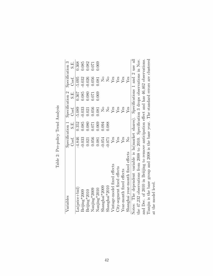
Tab

le2:

Pre

-pol

icy

Tre

nd

Anal

ysi

s

Var

iable

sSp

ecifi

cati

on1

Sp

ecifi

cati

on2

Sp

ecifi

cati

on3

Coef

.S.E

.C

oef

.S.E

.C

oef

.S.E

.L

n(p

rice

+bid

)-4

.846

0.35

2-5

.089

0.36

7-5

.095

0.36

8B

eiji

ng*

2009

-0.0

330.

085

-0.0

330.

085

-0.0

320.

085

Bei

jing*

2010

0.02

10.

080

0.02

10.

080

-0.0

260.

082

Nan

jing*

2009

0.05

60.

071

0.05

60.

071

0.05

60.

071

Nan

jing*

2010

0.08

10.

069

0.08

10.

069

0.08

10.

069

Shan

ghai

*200

9-0

.054

0.09

4N

oN

oShan

ghai

*201

0-0

.071

0.08

8N

oN

oV

inta

ge-m

odel

fixed

effec

tsY

esY

esY

esC

ity-s

egm

ent

fixed

effec

tsY

esY

esY

esY

ear-

mon

thfixed

effec

tsY

esY

esY

esShan

ghai

year

-mon

thfixed

effec

tsN

oY

esY

es

Not

es:

The

dep

enden

tva

riab

leis

ln(m

arke

tsh

ares

).Sp

ecifi

cati

ons

1an

d2

use

all

the

47,2

32ob

serv

atio

ns

from

2008

to20

10.

Sp

ecifi

cati

on3

dro

ps

obse

rvat

ions

inN

ov.

and

Dec

.of

2010

inB

eiij

ing

tore

mov

ean

tici

pat

ion

effec

tan

dhas

46,4

62ob

serv

atio

ns.

Tia

nji

nis

the

bas

egr

oup

and

2008

isth

ebas

eye

ar.

The

stan

dar

der

rors

are

clust

ered

atth

em

odel

leve

l.

42

Tab

le3:

Par

amet

erE

stim

ates

from

GM

M

Var

iab

les

Ben

chm

ark

Alt

ern

ativ

e1

Alt

ern

ativ

e2

Alt

ern

ativ

e3

Alt

ern

ati

ve4

Alt

ern

ati

ve5

Coef

.S

.E.

Coef

.S

.E.

Coef

.S

.E.

Coef

.S

.E.

Coef

.S

.E.

Coef

.S

.E.

Para

mete

rsin

the

hou

seh

old

-sp

ecifi

cu

tili

ty(θ

2)

Ln

(pri

ce+

bid

)-1

7.51

91.

927

-23.

687

2.04

1-8

.132

2.42

5-2

1.31

54.

133

-17.1

27

2.1

84

-16.2

22

1.8

52

Ln

(in

com

e)*l

n(p

+b

id)

1.55

80.

193

2.14

10.

256

-1.2

150.

403

1.56

10.

316

1.5

19

0.2

34

1.3

84

0.2

01

Ln

(in

com

e)-6

.442

0.89

7-7

.108

1.17

05.

850

1.92

6-6

.470

1.38

3-6

.387

1.1

40

-5.6

48

0.9

85

σfo

rln

(pri

ce+

bid

)0.

095

0.04

40.

195

0.05

90.

248

0.10

60.

215

0.08

40.0

80

0.0

63

0.0

91

0.0

56

σfo

rco

nst

ant

0.90

70.

261

0.01

10.

133

1.16

40.

543

1.51

20.

311

0.9

22

0.2

90

0.8

97

0.2

83

σfo

rfu

elco

sts/

100k

m0.

000

0.09

40.

000

0.06

00.

299

0.20

80.

002

0.11

90.0

03

0.1

20

0.0

01

0.1

14

σfo

rve

hic

lesi

ze0.

022

0.32

60.

020

0.15

50.

385

0.25

40.

065

0.19

30.1

37

0.4

98

0.0

65

0.5

17

σfo

ren

gin

ed

isp

lace

men

t1.

835

0.49

32.

954

0.33

72.

990

0.98

13.

726

1.02

31.3

60

0.5

55

1.5

20

0.5

61

Au

xilia

ryp

ara

mete

rsfo

rallocati

on

mech

an

ism

(θ3)

ρ0.

202

0.03

70.

395

0.03

00.

205

0.04

10.

283

0.03

60.1

82

0.0

33

0.1

86

0.0

41

γ0

-1.0

010.

018

-0.9

250.

042

-1.0

020.

038

-0.9

860.

343

-1.0

02

0.4

08

-1.0

04

0.0

65

γ1

0.25

20.

005

0.13

60.

006

0.24

80.

007

0.22

50.

078

0.2

53

0.1

03

0.2

55

0.0

17

Not

es:

Th

eb

ench

mar

km

od

elis

the

pre

ferr

edm

od

el.

Alt

ern

ativ

esp

ecifi

cati

on1

does

not

incl

ud

eth

efi

rst

set

of

mom

ent

con

dit

ion

s(c

omm

on-t

ren

dm

omen

ts).

Alt

ern

ativ

e2

does

not

incl

ud

eth

ese

con

dse

tof

mom

ent

con

dit

ion

s(m

icro

-mom

ents

).A

lter

nat

ive

3as

sum

esal

lth

eh

ouse

hol

ds

asth

ep

oten

tial

bu

yers

ina

year

soth

em

arke

tsi

zein

each

month

isth

eto

tal

nu

mb

erof

hou

seh

old

sd

ivid

edby

12.

Alt

ern

ativ

e4

assu

mes

ace

rtai

np

erce

nta

geof

lice

nse

sar

eu

sed

tob

uy

use

dve

hic

les:

15

per

cent

inB

eiji

ng

and

5p

erce

nt

inS

han

ghai

.A

lter

nat

ive

5ta

kes

the

ran

dom

dra

ws

for

un

obse

rved

hou

seh

old

att

rib

ute

sfr

om

ast

an

dard

nor

mal

dis

trib

uti

onre

mov

ing

dra

ws

bel

ow2.

5an

dab

ove

97.5

per

centi

les

43

Tab

le4:

Pol

icy

Impac

tson

Sal

esin

Bei

jing

and

Shan

ghai

Yea

rO

bse

rved

Sal

esC

ounte

rfac

tura

lS

ales

Ben

chm

ark

Alt

ern

ativ

e1

Alt

ern

ativ

e2

Alt

ern

ativ

e3

Alt

ern

ati

ve4

Alt

ern

ati

ve5

Beij

ing

2008

411,

936

411,

936

411,

936

411,

936

411,

936

411,9

36

411,9

36

2009

602,

219

602,

219

602,

219

602,

219

602,

219

602,2

19

602,2

19

2010

804,

355

804,

355

804,

355

804,

355

804,

355

804,3

55

804,3

55

2011

334,

308

779,

273

591,

789

774,

600

691,

476

800,6

55

797,0

41

2012

520,

442

1,14

2,06

488

4,54

11,

114,

074

1,00

4,96

91,

177,8

13

1,1

70,6

55

Sh

an

gh

ai

2008

165,

298

344,

955

322,

379

340,

356

377,

179

346,2

77

340,9

70

2009

208,

570

414,

994

417,

469

399,

754

453,

940

418,8

68

412,8

30

2010

264,

232

577,

542

538,

468

567,

164

651,

788

575,7

82

568,7

14

2011

277,

119

599,

425

603,

846

597,

196

603,

463

609,9

72

599,9

61

2012

295,

047

712,

215

681,

951

688,

113

779,

833

723,1

97

712,2

05

Not

es:

Th

esi

xco

unte

rfac

tual

outc

omes

corr

esp

ond

toth

esi

xsp

ecifi

cati

ons

inT

able

3.

44

Table 5: Welfare Comparison Between Lottery and Auction in Beijing

15-year Horizon 10-year HorizonLottery Auction Lottery Auction

(1) (2) (3) (4)

Observed Quota LevelQuota in 2012 259,800 259,800 259,800 259,800Clearing price (in 1000 RMB) 0.00 82.21 0.00 82.21Realized consumer surplus (in billion) 5.39 48.35 5.39 48.35Unrealized consumer surplus (in billon) 42.96 0.00 42.96 0.00

Average fuel economy (liters per 100km) 8.92 9.19 8.92 9.19Annual VMT (1000 kms) 17.76 19.80 17.76 19.80Total external costs (in billion) 33.02 40.21 24.57 29.92

Government revenue (in billion) 0.00 21.36 0.00 21.36Net social welfare (in billion) -27.63 8.13 -19.18 18.43

Optimal Quota LevelOptimal quota 125,612 183,796Clearing price (in 1000) 157.50 112.50Consumer surplus (in billion) 34.87 42.60Total external costs (in billion) 20.75 21.82Government revenue (in billion) 19.78 20.68Net social welfare (in billion) 14.12 20.79

Notes: All monetary variables are in RMB ($1 for about 6.1 RMB). The top panelpresents welfare comparison between a lottery system and a uniform price auctionfor Beijing in 2012. The bottom panel shows welfare outcomes with the optimallevels of quota. The optimal quotas are defined by the intersections between thevertical dashed line and the downward sloping dashed line in the two panels ofFigure 4. Net social welfare is equal to realized consumer surplus minus totalexternal costs. Columns (1) and (2) use a 15-year time span for calculating totalexternal costs, i.e., total discounted external costs during 15 years with a discountrate of 5%. Columns (3) and (4) are results based on a 10-year time span forexternal costs.

45

Appendices

NOT FOR PUBLICATION: ONLINE MATERIALS

Figure 1: New Vehicle Sales in China and Vehicle Stocks in Beijng and Shanghai

Notes: The top panel depicts annual sales of new passenger vehicles in China and the U.S.from 2001 to 2012. The bottom panel shows the vehicle stock of passenger vehicles in Beijingand Shanghai from 2003 to 2012.

1

Fig

ure

2:M

onth

lyV

ehic

leSal

esan

dN

um

ber

oflice

nse

sin

Bei

jing

and

Shan

ghai

01

/08

06

/08

12

/08

06

/09

12

/09

06

/10

12

/10

06

/11

12

/11

06

/12

12

/12

05

10

15

x 1

04

Be

ijin

g S

ale

s

Pe

rmits

01

/08

06

/08

12

/08

06

/09

12

/09

06

/10

12

/10

06

/11

12

/11

06

/12

12

/12

01234567x 1

04

Sh

an

gh

ai S

ale

s

Pe

rmits

Ave

rag

e P

rice

Lo

we

st

Price

2

Tab

le1:

Cit

yC

har

acte

rist

ics

inB

eiji

ng,

Nan

jing,

Shan

ghai

,T

ianji

n

Yea

rC

ity

No.

ofH

ouse

hol

ds

Ave

rage

Hou

sehol

dN

ewve

hic

leN

atio

nal

Veh

icle

%in

nat

ion

(mil.)

Inco

me

(in

RM

B)

Sal

esSal

es(m

il.)

2008

Bei

jing

605.

9969

,230

419,

703

6.76

6.21

2009

Bei

jing

636.

2974

,866

610,

076

10.3

35.

9120

10B

eiji

ng

668.

1081

,404

815,

211

13.7

65.

9320

11B

eiji

ng

687.

8688

,838

346,

207

14.4

72.

3920

12B

eiji

ng

704.

8998

,466

536,

216

15.5

03.

4620

08N

anji

ng

224.

6862

,431

83,4

596.

761.

2420

09N

anji

ng

230.

8468

,861

131,

316

10.3

31.

2720

10N

anji

ng

237.

0076

,442

177,

105

13.7

61.

2920

11N

anji

ng

240.

0886

,940

166,

770

14.4

71.

1520

12N

anji

ng

241.

6298

,069

187,

194

15.5

01.

2120

08Shan

ghai

774.

1279

,225

169,

678

6.76

2.51

2009

Shan

ghai

799.

2184

,495

212,

139

10.3

32.

0520

10Shan

ghai

825.

1092

,330

268,

507

13.7

61.

9520

11Shan

ghai

841.

2310

5,06

728

4,69

314

.47

1.97

2012

Shan

ghai

853.

0611

6,54

530

3,09

515

.50

1.96

2008

Tia

nji

n34

7.88

56,1

3116

0,22

16.

762.

3720

09T

ianji

n35

6.92

61,7

3722

3,77

410

.33

2.17

2010

Tia

nji

n36

6.20

69,4

7727

6,71

613

.76

2.01

2011

Tia

nji

n38

3.35

76,4

5527

8,33

614

.47

1.92

2012

Tia

nji

n39

9.92

84,1

3829

2,44

215

.50

1.89

Not

es:

The

sale

sdat

aar

efr

omR

.L.P

olk

&C

O.an

dot

her

vari

able

sar

efr

omva

riou

sis

sues

ofA

nnual

Soci

alan

dE

conom

icD

evel

opm

ent

Rep

ort

by

each

ofth

eci

ties

.T

he

aver

age

inco

me

isnom

inal

.N

ewve

hic

lesa

les

incl

ude

pas

senge

rca

rsan

dligh

ttr

uck

s.

3

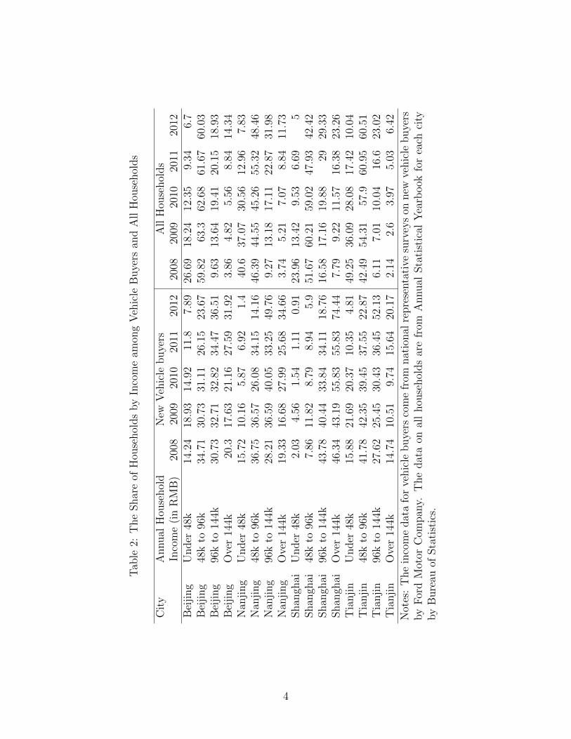
Tab

le2:

The

Shar

eof

Hou

sehol

ds

by

Inco

me

amon

gV

ehic

leB

uye

rsan

dA

llH

ouse

hol

ds

Cit

yA

nnual

Hou

sehol

dN

ewV

ehic

lebuye

rsA

llH

ouse

hol

ds

Inco

me

(in

RM

B)

2008

2009

2010

2011

2012

2008

2009

2010

2011

2012

Bei

jing

Under

48k

14.2

418

.93

14.9

211

.87.

8926

.69

18.2

412

.35

9.34

6.7

Bei

jing

48k

to96

k34

.71

30.7

331

.11

26.1

523

.67

59.8

263

.362

.68

61.6

760

.03

Bei

jing

96k

to14

4k30

.73

32.7

132

.82

34.4

736

.51

9.63

13.6

419

.41

20.1

518

.93

Bei

jing

Ove

r14

4k20

.317

.63

21.1

627

.59

31.9

23.

864.

825.

568.

8414

.34

Nan

jing

Under

48k

15.7

210

.16

5.87

6.92

1.4

40.6

37.0

730

.56

12.9

67.

83N

anji

ng

48k

to96

k36

.75

36.5

726

.08

34.1

514

.16

46.3

944

.55

45.2

655

.32

48.4

6N

anji

ng

96k

to14

4k28

.21

36.5

940

.05

33.2

549

.76

9.27

13.1

817

.11

22.8

731

.98

Nan

jing

Ove

r14

4k19

.33

16.6

827

.99

25.6

834

.66

3.74

5.21

7.07

8.84

11.7

3Shan

ghai

Under

48k

2.03

4.56

1.54

1.11

0.91

23.9

613

.42

9.53

6.69

5Shan

ghai

48k

to96

k7.

8611

.82

8.79

8.94

5.9

51.6

760

.21

59.0

247

.93

42.4

2Shan

ghai

96k

to14

4k43

.78

40.4

433

.84

34.1

118

.76

16.5

817

.16

19.8

829

29.3

3Shan

ghai

Ove

r14

4k46

.34

43.1

955

.83

55.8

374

.44

7.79

9.22

11.5

716

.38

23.2

6T

ianji

nU

nder

48k

15.8

821

.69

20.3

710

.35

4.81

49.2

536

.09

28.0

817

.42

10.0

4T

ianji

n48

kto

96k

41.7

842

.35

39.4

537

.55

22.8

742

.49

54.3

157

.960

.95

60.5

1T

ianji

n96

kto

144k

27.6

225

.45

30.4

336

.45

52.1

36.

117.

0110

.04

16.6

23.0

2T

ianji

nO

ver

144k

14.7

410

.51

9.74

15.6

420

.17

2.14

2.6

3.97

5.03

6.42

Not

es:

The

inco

me

dat

afo

rve

hic

lebuye

rsco

me

from

nat

ional

repre

senta

tive

surv

eys

onnew

vehic

lebuye

rsby

For

dM

otor

Com

pan

y.T

he

dat

aon

all

hou

sehol

ds

are

from

Annual

Sta

tist

ical

Yea

rbook

for

each

city

by

Bure

auof

Sta

tist

ics.

4

Tab

le3:

Sal

esIm

pac

tsof

the

Lot

tery

Pol

icy

inB

eiji

ng

Var

iable

sSp

ecifi

cati

on1

Sp

ecifi

cati

on2

Sp

ecifi

cati

on3

Coef

.S.E

.Im

pac

tsC

oef

.S.E

.Im

pac

tsC

oef

.S.E

.Im

pac

tsL

n(p

rice

+bid

)-3

.213

0.17

4-3

.229

0.17

44-3

.229

0.17

5L

otte

ryin

2011

-0.9

380.

116

-60.

6%-0

.787

0.12

2-5

4.1

%-0

.803

0.04

6-5

5.1%

Lot

tery

in20

12-0

.730

0.21

3-5

0.7

%-0

.543

0.22

16-4

0.5%

-0.5

470.

046

-42.

1%V

inta

ge-m

odel

fixed

effec

tsY

esY

esY

esY

ear-

mon

thfixed

effec

tsY

esY

esY

esShan

ghai

*ye

ar-m

onth

effec

tsY

esY

esY

esC

ity-s

egm

ent

fixed

effec

tsY

esY

esY

esC

ity

tren

d(q

uad

rati

c)Y

esY

esN

o

Not

es:

The

dep

enden

tva

riab

leis

ln(m

arke

tsh

ares

).Sp

ecifi

cati

ons

1use

all

the

84,9

12ob

serv

atio

ns

from

2008

to20

12.

Sp

ecifi

cati

ons

2an

d3

dro

pth

ela

sttw

om

onth

sin

2010

and

firs

ttw

om

onth

sof

2011

for

Bei

jing

tore

mov

ean

tici

pat

ion

effec

t.T

he

stan

dar

der

rors

are

clust

ered

atth

em

odel

leve

l.

5