Embed Size (px)
Citation preview

University of MiamiScholarly Repository
Open Access Dissertations Electronic Theses and Dissertations
2008-04-12
Bethe Ansatz and Open Spin-1/2 XXZ QuantumSpin ChainRajan MurganUniversity of Miami, [email protected]
Follow this and additional works at: https://scholarlyrepository.miami.edu/oa_dissertations
This Open access is brought to you for free and open access by the Electronic Theses and Dissertations at Scholarly Repository. It has been accepted forinclusion in Open Access Dissertations by an authorized administrator of Scholarly Repository. For more information, please [email protected].
Recommended CitationMurgan, Rajan, "Bethe Ansatz and Open Spin-1/2 XXZ Quantum Spin Chain" (2008). Open Access Dissertations. 69.https://scholarlyrepository.miami.edu/oa_dissertations/69


UNIVERSITY OF MIAMI
BETHE ANSATZ AND OPEN SPIN-12
XXZ QUANTUM SPIN CHAIN
By
Rajan Murgan
A DISSERTATION
Submitted to the Facultyof the University of Miami
in Partial Fulfillment of the Requirements forthe Degree of Doctor of Philosophy
Coral Gables, Florida
May 2008

UNIVERSITY OF MIAMI
A dissertation submitted in partial fulfillment ofthe requirements for the degree of
Doctor of Philosophy
BETHE ANSATZ AND OPEN SPIN-12
XXZ QUANTUM SPIN CHAIN
Rajan Murgan
Approved:
Dr. Rafael Nepomechie Dr. Terri A. ScanduraProfessor of Physics Dean of the Graduate School
Dr. Orlando Alvarez Dr. James NearingProfessor of Physics Professor of Physics
Dr. Changrim AhnProfessor of PhysicsEwha Womans University

RAJAN MURGAN (Ph.D., Physics)
Bethe Ansatz and Open Spin-12
XXZ
Quantum Spin Chain (May 2008)
Abstract of a dissertation at the University of Miami.
Dissertation supervised by Professor Rafael I. NepomechieNo. of page in text. (141)
The open spin-12
XXZ quantum spin chain with general integrable boundary
terms is a fundamental integrable model. Finding a Bethe Ansatz solution for this
model has been a subject of intensive research for many years. Such solutions for
other simpler spin chain models have been shown to be essential for calculating
various physical quantities, e.g., spectrum, scattering amplitudes, finite size cor-
rections, anomalous dimensions of certain field operators in gauge field theories,
etc.
The first part of this dissertation focuses on Bethe Ansatz solutions for open
spin chains with nondiagonal boundary terms. We present such solutions for some
special cases where the Hamiltonians contain two free boundary parameters. The
functional relation approach is utilized to solve the models at roots of unity, i.e.,
for bulk anisotropy values η = iπp+1
where p is a positive integer. This approach
is then used to solve open spin chain with the most general integrable boundary
terms with six boundary parameters, also at roots of unity, with no constraint
among the boundary parameters.
The second part of the dissertation is entirely on applications of the newly
obtained Bethe Ansatz solutions. We first analyze the ground state and compute

the boundary energy (order 1 correction) for all the cases mentioned above. We
extend the analysis to study certain excited states for the two-parameter case. We
investigate low-lying excited states with one hole and compute the corresponding
Casimir energy (order 1N
correction) and conformal dimensions for these states.
These results are later generalized to many-hole states. Finally, we compute the
boundary S-matrix for one-hole excitations and show that the scattering ampli-
tudes found correspond to the well known results of Ghoshal and Zamolodchikov
for the boundary sine-Gordon model provided certain identifications between the
lattice parameters (from the spin chain Hamiltonian) and infrared (IR) parameters
(from the boundary sine-Gordon S-matrix) are made.

To my parents
iii

ACKNOWLEDGEMENTS
I wish to express my deepest gratitude to my thesis advisor, Professor R.I.
Nepomechie, who introduced me to the subject of Bethe Ansatz and integrable
models. I deeply appreciate the invaluable guidance, patience and support that he
provided throughout my doctoral studies. I also would like to thank the Depart-
ment of Physics and College of Arts and Sciences at the University of Miami for
their continuous financial support.
iv

TABLE OF CONTENTS
1 Chapter 1: Introduction . . . . . . . . . . . . . . . . . . . . . . . . . . . 1
1.1 Conditions of integrability . . . . . . . . . . . . . . . . . . . . . . . 3
1.1.1 Yang-Baxter equation . . . . . . . . . . . . . . . . . . . . . 3
1.1.2 Boundary Yang-Baxter equation . . . . . . . . . . . . . . . . 4
1.2 Spin-12
XXZ quantum spin chains . . . . . . . . . . . . . . . . . . . 4
1.2.1 Closed spin chain . . . . . . . . . . . . . . . . . . . . . . . . 5
1.2.2 Open spin chain . . . . . . . . . . . . . . . . . . . . . . . . . 6
1.3 Algebraic Bethe Ansatz . . . . . . . . . . . . . . . . . . . . . . . . . 6
1.4 McCoy’s method . . . . . . . . . . . . . . . . . . . . . . . . . . . . 8
2 Chapter 2: Bethe Ansatz For Special Cases of an
Open XXZ Spin Chain . . . . . . . . . . . . . . . . . . . . . 12
2.1 Transfer matrix and functional relations . . . . . . . . . . . . . . . 14
2.2 Bethe Ansatz solution: Even p, one arbitrary boundary parameter . 18
2.2.1 α− 6= 0 . . . . . . . . . . . . . . . . . . . . . . . . . . . . . . 18
2.2.2 β− 6= 0 . . . . . . . . . . . . . . . . . . . . . . . . . . . . . . 21
2.2.3 θ∓ 6= 0 . . . . . . . . . . . . . . . . . . . . . . . . . . . . . . 22
2.3 Bethe Ansatz solution: Even p, two arbitrary boundary parameters 24
2.3.1 α− , α+ arbitrary . . . . . . . . . . . . . . . . . . . . . . . . 25
2.3.2 β− , β+ arbitrary . . . . . . . . . . . . . . . . . . . . . . . . 26
2.3.3 α− , β− arbitrary . . . . . . . . . . . . . . . . . . . . . . . . 26
v

2.4 Bethe Ansatz solution: Odd p, two arbitrary boundary parameters . 28
2.5 An attempt to obtain a conventional T −Q relation . . . . . . . . . 29
2.6 The generalized T −Q relations . . . . . . . . . . . . . . . . . . . . 32
2.6.1 α− 6= 0, β− 6= 0 and α+ = β+ = θ± = 0 . . . . . . . . . . . . 34
2.6.2 α± 6= 0 and β± = θ± = 0 . . . . . . . . . . . . . . . . . . . . 36
3 Chapter 3: Bethe Ansatz For General Case of an
Open XXZ Spin Chain . . . . . . . . . . . . . . . . . . . . . 39
3.1 The case p > 1 . . . . . . . . . . . . . . . . . . . . . . . . . . . . . 40
3.1.1 The matrix M(u) . . . . . . . . . . . . . . . . . . . . . . . . 40
3.1.2 Bethe Ansatz . . . . . . . . . . . . . . . . . . . . . . . . . . 45
3.2 The XX chain (p = 1) . . . . . . . . . . . . . . . . . . . . . . . . . 50
4 Chapter 4: Boundary Energy of The Open XXZ Chain
From New Exact Solutions . . . . . . . . . . . . . . . . . . . 56
4.1 Case I: p even . . . . . . . . . . . . . . . . . . . . . . . . . . . . . . 57
4.2 Case II: p odd . . . . . . . . . . . . . . . . . . . . . . . . . . . . . . 65
5 Chapter 5: Boundary Energy of The General Open
XXZ Chain at Roots of Unity . . . . . . . . . . . . . . . . . 73
5.1 Bethe Ansatz . . . . . . . . . . . . . . . . . . . . . . . . . . . . . . 74
5.2 Even p . . . . . . . . . . . . . . . . . . . . . . . . . . . . . . . . . . 77
5.2.1 Sea roots {v±(aj)k , v
±(bj)k } . . . . . . . . . . . . . . . . . . . . 78
5.2.2 Extra roots {w±(aj ,l)k , w
±(bj)k } . . . . . . . . . . . . . . . . . . 78
5.2.3 Boundary energy . . . . . . . . . . . . . . . . . . . . . . . . 79
5.3 Odd p . . . . . . . . . . . . . . . . . . . . . . . . . . . . . . . . . . 84
5.3.1 Sea roots {v±(aj)k , v
±(bj)k } . . . . . . . . . . . . . . . . . . . . 85
5.3.2 Extra roots {w(aj ,l)k , w
(bj)k } . . . . . . . . . . . . . . . . . . . 85
vi

5.3.3 Boundary energy . . . . . . . . . . . . . . . . . . . . . . . . 87
6 Chapter 6: Finite-Size Correction and Bulk Hole-Excitations . . . . . . . 93
6.1 Bethe Ansatz . . . . . . . . . . . . . . . . . . . . . . . . . . . . . . 95
6.1.1 Even N . . . . . . . . . . . . . . . . . . . . . . . . . . . . . 95
6.1.2 Odd N . . . . . . . . . . . . . . . . . . . . . . . . . . . . . . 96
6.2 Finite-size correction of order 1/N . . . . . . . . . . . . . . . . . . . 97
6.2.1 Sum-rule and hole-excitations . . . . . . . . . . . . . . . . . 98
6.2.2 Casimir energy . . . . . . . . . . . . . . . . . . . . . . . . . 103
6.3 Numerical results . . . . . . . . . . . . . . . . . . . . . . . . . . . . 108
7 Chapter 7: Boundary S Matrix . . . . . . . . . . . . . . . . . . . . . . . 111
7.1 One-hole state . . . . . . . . . . . . . . . . . . . . . . . . . . . . . . 113
7.2 One-hole state with 2-string . . . . . . . . . . . . . . . . . . . . . . 114
7.3 Boundary S matrix . . . . . . . . . . . . . . . . . . . . . . . . . . . 116
7.3.1 Eigenvalue for the one-hole state without 2-string . . . . . . 116
7.3.2 Eigenvalue for the one-hole state with 2-string . . . . . . . . 121
7.3.3 Relation to boundary sine-Gordon model . . . . . . . . . . . 123
Appendix 1 . . . . . . . . . . . . . . . . . . . . . . . . . . . . . . . . . . . . 127
Appendix 2 . . . . . . . . . . . . . . . . . . . . . . . . . . . . . . . . . . . . 129
Appendix 3 . . . . . . . . . . . . . . . . . . . . . . . . . . . . . . . . . . . . 131
3.0.4 Case I: p even . . . . . . . . . . . . . . . . . . . . . . . . . . 131
3.0.5 Case II: p odd . . . . . . . . . . . . . . . . . . . . . . . . . . 132
Bibliography . . . . . . . . . . . . . . . . . . . . . . . . . . . . . . . . . . . 133
vii

Chapter 1: Introduction
Exact solutions to some fundamental physical systems such as the hydrogen
atom and the harmonic oscillator have played crucial roles in the development of
physics. Sytems that can be solved exactly are said to be “integrable.” Such exact
solutions allow many of the physical properties of these systems such as the spec-
trum, scattering amplitudes, correlation functions, etc., to be determined exactly
without resorting to any sort of approximation methods. Historically, Yang [1]
in his solution of the problem of particles in one dimension with repulsive delta
function interaction and Baxter [2] in his solution of the eight vertex statistical
model independently showed that these integrable models satisfy a special non-
linear equation, known as the Yang-Baxter equation (YBE). This equation is a
crucial condition of integrability. The YBE also arises as the condition of factor-
izability of the multiparticle S-matrix of 1 + 1 dimensional integrable quantum
field theory models, such as the sine-Gordon model [3]. For systems with bound-
ary, Zamolodchikov and Cherednik [4, 5] introduced the reflection equation, also
known as the boundary Yang-Baxter equation (BYBE), that ensures boundary
integrability. Ghoshal and Zamolodchikov [6] demonstrated such boundary inte-
grability in certain 1 + 1 dimensional boundary quantum field theories through
their formulation of boundary scattering matrices that obey BYBE.
A quantum spin chain is a fundamental prototype of integrable models. Such
chains come with two topologies, “closed” and “open.” Originally, Heisenberg
[7] introduced the isotropic closed spin-12
XXX quantum spin chain in 1928. A
few years later, Bethe proposed an ansatz, called Bethe’s hypothesis, to solve
1
2
the model [8]. Hulthen studied the antiferromagnetic ground state of this model
[9] using Bethe’s hypothesis. This method, now known as the coordinate Bethe
Ansatz, was later used by others to obtain further important results on closed
spin-12
XXX and XXZ (anisotropic) spin chains [10]–[13]. Gaudin and Alcaraz et
al. utilized the method to solve the open spin-12
XXZ quantum spin chain with
diagonal boundary terms [14, 15] It also served as an important tool to study other
models, e.g. delta-function interaction problem [16].
Bethe Ansatz has since been a powerful method to solve integrable models.
Over the years, it has been subjected to numerous investigations and applied to
solve many quantum systems. In the late 1970’s, an alternative method with
common mathematical background to coordinate space Bethe Ansatz was devised.
This method, which relies on diagonalization of transfer matrices, is known as the
Quantum Inverse Scattering Method (QISM) or the algebraic Bethe ansatz (ABA)
[17]–[22]. It requires a reference state from which the desired Bethe states can
be constructed. ABA has been used to solve many simpler quantum spin chain
models, e.g., open spin-12
XXZ quantum spin chain with diagonal boundary terms
[23]. However, obtaining such a reference state for more general quantum spin
chains has proven to be a formidable task and still is an open problem. Recently,
an ABA solution for the corresponding open spin chain with nondiagonal boundary
terms with constrained boundary parameters was proposed [24], where a proper
“reference” state for this model was found. This Bethe Ansatz solution was also
derived using certain functional relations [27, 28] and the Q-operator [29], which
do not require the construction of reference states.
We note that Bethe Ansatz is only one of the possible routes towards integra-
bility. Recently, Baseilhac and Koizumi [30] and Galleas [31] proposed solutions
for the generic case of the open spin-12
XXZ quantum spin chain using q-Onsager

3
algebra and nonlinear algebraic relations, respectively. However, computations
of thermodynamic properties such as finite size corrections and S-matrices using
these methods are still unclear at the present. In this dissertation, we restrict
our investigation of integrable quantum spin chains using strictly Bethe-Ansatz-
type solutions derived from functional relations. In the following sections of this
chapter, some of the above-mentioned results will be briefly reviewed.
1.1 Conditions of integrability
For quantum integrable models, YBE and BYBE ensure bulk and boundary
(for models involving boundaries) integrability, respectively. These are nonlinear
equations involving R(u) and K(u) matrices, which are the solutions of these
equations 1. The matrix R(u) is defined as an operator acting on the tensor
product space V ⊗V , where V generally is a N -dimensional complex vector space
CN . Similarly, the matrix K(u) is defined as an operator acting on V . We review
them separately below.
1.1.1 Yang-Baxter equation
We first define the permutation matrix, Px ⊗ y = y ⊗ x for all vectors x and
y. The YBE can be written as
R12(u− v)R13(u)R23(v) = R23(v)R13(u)R12(u− v) (1.1)
where Rij are operators on V ⊗ V ⊗ V , with R12 = R ⊗ 1 , R23 = 1 ⊗ R and
R13 = P23R12P23, where P23 = 1⊗P is the permutation matrix acting nontrivially
on the second and third spaces and trivially on the first. Evidently, R12 acts
nontrivially on the first and second spaces and trivially on the third. Similarly,
R13 acts nontrivially on the first and third spaces and trivially on the second, etc.
1Studies on YBE and BYBE and their solutions have significantly advanced the subject ofquantum groups, where these solutions arise from the representations of the quantum groups.

4
The independent variable u (or v) is called the “spectral parameter.” One can
interpret (1.1) as factorized scattering of three particles in bulk [3]. As we shall
see, the trigonometric solution with V = C2 of the YBE is of particular interest to
us since it yields the R matrix of the spin-12
XXZ quantum spin chain given below,
R(u) =
a 0 0 00 b c 00 c b 00 0 0 a
, (1.2)
where
a = sinh(u + η) , b = sinh u , c = sinh η (1.3)
and η is the bulk anisotropy parameter.
1.1.2 Boundary Yang-Baxter equation
The BYBE can be written as [4, 5]
R12(u− v)K1(u)R21(u + v)K2(v) = K2(v)R12(u + v)K1(u)R21(u− v) (1.4)
where Rij is defined as before. The matrix K(u) acts on space V , with K1 =
K ⊗ 1 , K2 = 1⊗K. As usual, u and v are spectral parameters. Analogous to the
YBE (1.1), the BYBE (1.4) can be seen as scattering of particles from a boundary.
As for the YBE, various solutions of the BYBE have been found. The most general
matrix K(u) of the open spin-12
XXZ quantum spin chain was found by de Vega
and Gonzalez-Ruiz [32] and independently by Goshal and Zamolodchikov [6] by
solving (1.4) directly using the R matrix (1.2).
1.2 Spin-12 XXZ quantum spin chains
Construction of spin chains requires two crucial “building blocks”, namely the
R and K matrices introduced above. In the following sections, we review the

5
construction of both the closed and open spin-12
XXZ quantum spin chains from
these matrices.
1.2.1 Closed spin chain
The closed spin-12
XXZ chain is constructed from only the R matrix (1.2). The
transfer matrix can be expressed as
t(u) = tr0 T0(u) (1.5)
where T0(u) is the monodromy matrix defined as a product of R matrices,
T0(u) = R0N(u) · · ·R01(u) (1.6)
where R0n(u) is an operator on
0
↓V ⊗
1
↓V · · · ⊗
n
↓V ⊗ · · ·⊗
N
↓V (1.7)
where “0” is the “auxiliary space” over which the trace tr0 is taken, and n takes the
values of 1 , 2 . . . , N representing the “quantum spaces.” The monodromy matrix
obeys the fundamental relation
R00′(u− v)T0(u)T0′(v) = T0′(v)T0(u)R00′(u− v) (1.8)
which can be proven using (1.1) and the fact that R0n commutes with R0′n′ for
n 6= n′. The transfer matrix has the following important commutativity property
[t(u), t(v)] = 0 (1.9)
The Hamiltonian can be constructed from the logarithmic derivative of the transfer
matrix,
H = sinh ηd
dulog t(u)|u=0 −
N
2cosh ηI

6
=N−1∑n=1
Hn,n+1 + HN,1 ,
Hij = sinh ηPijR′ij(0)−
1
2cosh ηI
=1
2
(σx
nσxn+1 + σy
nσyn+1 + cosh η σz
nσzn+1
)(1.10)
where σx , σy , σz are the standard Pauli matrices, η is the bulk anisotropy parame-
ter, and the prime indicates differentiation with respect to the spectral parameter.
One then can readily conclude that [H, t(u)] = 0.
1.2.2 Open spin chain
The transfer matrix t(u) of the open spin chain is given by [23]
t(u) = tr0 K+0 (u)T0(u)K−
0 (u)T0(u), (1.11)
where T0(u) and T0(u) are the monodromy matrices,
T0(u) = R0N(u) · · ·R01(u) , T0(u) = R01(u) · · ·R0N(u), (1.12)
and tr0 again denotes trace over the “auxiliary space” 0. K+(u) and K−(u) are
the K matrices corresponding to the left and right boundaries of the open spin
chain, respectively. One can relate the transfer matrix to the open spin chain
Hamiltonian H using (see [23])
t′(0) = 2H tr K+(0) + tr K+(0)′ (1.13)
More discussions on these subjects are found in subsequent chapters where solu-
tions of open XXZ spin chains and applications of these solutions are presented.
1.3 Algebraic Bethe Ansatz
In this section, we review the ABA approach, applied to the case of the closed
spin-12
XXZ spin chain. A crucial element to this approach is the R matrix (1.2)
7
discussed above. Detailed information on this approach can be found in [22]. The
monodromy matrix T0(u) is a 2× 2 matrix in the auxiliary space,
T0(u) =
(A(u) B(u)C(u) D(u)
), (1.14)
where the elements of this matrix are operators acting on the quantum space V ⊗N .
These operators obey the following set of algebraic relations encoded in (1.8),
[B(u), B(v)] = 0
A(u)B(v) =a(v − u)
b(v − u)B(v)A(u)− c(v − u)
b(v − u)B(u)A(v) ,
D(u)B(v) =a(u− v)
b(u− v)B(v)D(u)− c(u− v)
b(u− v)B(u)D(v) , (1.15)
where a, b and c are given by (1.3).
The following reference state ω+ (ferromagnetic state with all spins up) is an
eigenstate of A(u) and D(u)
ω+ =
(10
)⊗ · · · ⊗
(10
)︸ ︷︷ ︸
N
(1.16)
namely,
A(u)ω+ = sinhN(u + η)ω+ , D(u)ω+ = sinhN(u)ω+ (1.17)
Further, it is annihilated by C(u), C(u)ω+ = 0. B(u) can be used as a creation
operator to form so-called Bethe states,
B(u1) · · ·B(uM)ω+ = |u1, . . . , uM〉. (1.18)
From (1.5), (1.14)-(1.18), it can be shown that the Bethe state |u1, . . . , uM〉 is an
eigenstate of the transfer matrix t(u) = A(u) + D(u),
t(u)|u1, . . . , uM〉 = Λ(u; u1, . . . , uM)|u1, . . . , uM〉 (1.19)
8
with the eigenvalue
Λ(u; u1, . . . , uM) = sinhN(u + η)Q(u− η)
Q(u)+ sinhN(u)
Q(u + η)
Q(u)(1.20)
provided the zeros uα of the function
Q(u) =M∏
α=1
sinh(u− uα) (1.21)
satisfy the following Bethe Ansatz equations,
(sinh(uβ + η)
sinh(uβ)
)N= −
M∏α=1
sinh(uβ − uα + η)
sinh(uβ − uα − η)β = 1, . . . ,M,
0 ≤ M ≤ N
2(1.22)
which also naturally arise from the analyticity of the eigenvalue Λ(u; u1, . . . , uM).
Quantities of interest such as the energy can now be calculated from the solution
of (1.22) using
E = sinh2 ηM∑
α=1
1
sinh(uα + η) sinh(uα)+
N
2cosh η (1.23)
which can be derived from (1.10) and (1.20). Equations (1.20) and (1.22) are
the desired solution of this model that one could use to compute further various
physical quantities of the quantum spin chain e.g., bulk scattering amplitudes of
spinons. In the following chapters, we shall derive such Bethe Ansatz type equa-
tions for more general open quantum XXZ spin chains and utilize these solutions
to determine various important physical quantities. Completeness of these solu-
tions can be numerically checked for small number of sites using a method which
we describe below.
1.4 McCoy’s method
In this section, we describe a method pioneered by Barry McCoy and his
collaborators [33, 34], known as ‘McCoy’s method’, to check completeness of Bethe

9
Ansatz type solutions. It is based on the transfer matrix of the model. One works
with newly defined spectral parameters, x ≡ eu and bulk anisotropy parameter,
q ≡ eη. McCoy’s method consists of four main steps (cf.[28]):
(a) We fix an arbitrary (generic) value x0 of the spectral parameter, for which
we compute the eigenvectors |Λ〉 of the transfer matrix t(x0). These eigenvectors
are independent of the spectral parameter (due to the commutativity property of
the transfer matrix (1.9)).
(b) Next, we determine the eigenvalues Λ(x) as Laurent polynomials in x by
acting with t(x) on the eigenvectors found in (a).
(c) We further set Q(x) =∑M
k=−M akxk (from (1.21)), and determine the coeffi-
cients ak from the relation (1.20), i.e., Λ(x)Q(x) = h(xq)Q(xq) + h(x)Q(xq), where
h(x) = (x−x−1
2)N .
(d) Finally, we factor the polynomials Q(x), the zeros of which are the Bethe
roots one is looking for.
We tabulate results (energy and Bethe roots) for the ground state of the closed
spin-12
XXZ quantum spin chain with even N , obtained using this method in Table
1.1. We also demonstrate the completeness of the solution (1.22) numerically for
N = 4 in Table 1.2. The number of Bethe roots M is not fixed and is related to
the spin Sz,
Sz = ±(N
2−M) (1.24)
The “±” can be attributed to the charge conjugation symmetry of the model.
This symmetry also implies a two-fold degeneracy of states with nonzero Sz, e.g.,
in Table 1.2., states with E = −2.0 and 2.0 are two-fold degenerate, with spin
Sz = ±1. Another example is the reference state with all spin up (or down) with
M = 0, namely Sz = +2 (or Sz = −2) which also gives the two-fold degeneracy.
The nondegenerate states, e.g., E = −3.62258 and 2.20837 have Sz = 0, giving

10
M = 2. Finally, note that there also exist states with much higher degeneracy,
e.g., E = 0. For these states, in addition to energy and spin, other quantities like
the momentum should be taken into consideration to distinguish them.
N M ground state energy, E shifted Bethe roots uα = uα + η2
2 1 -2.70711 04 2 -3.62258 -0.226301, 0.2263016 3 -5.08036 -0.336515, 0, 0.3365158 4 -6.61973 -0.411590, -0.101612, 0.101612, 0.411590
Table 1.1: Ground state energy and Bethe roots of the closed spin-12
XXZ chainin the massless regime (imaginary η), for η = iπ
4.
Energy, E degeneracy M shifted Bethe roots uα = uα + η2
-3.62258 1 2 -0.226301, 0.226301-2.0 2 1 0
1 0-1.41421 1 2 0 , iπ
2
0 7 1 -0.4406871 -0.4406871 0.4406871 0.4406872 -0.329239 + iπ
2, 0.329239
2 0.329239 + iπ2, -0.329239
2 -η2, η
2
1.41421 2 0 -0 -
2.0 2 1 iπ2
1 iπ2
2.20837 1 2 ± 0.600211 + iπ2
Table 1.2: Complete set of 24 energy levels and Bethe roots of the closed spin-12
XXZ chain in the massless regime, for η = iπ4.

11
Subsequent chapters of this dissertation consists of the following papers:
Chapter 2 “Bethe ansatz from functional relations of open XXZ chain for new
special cases”, JSTAT P05007 (2005), Addendum JSTAT P11004 (2005) and
“Generalized T-Q relations and the open XXZ chain”, JSTAT P08002 (2005) by
R. Murgan and R.I. Nepomechie.
Chapter 3 “Exact solution of the open XXZ chain with general integrable bound-
ary terms at roots of unity”, JSTAT P08006 (2006) by R. Murgan, R.I. Nepomechie
and Chi Shi.
Chapter 4 “Boundary energy of the open XXZ chain from new exact solutions”,
Annales Henri Poincare 7 (2006) 1429 by R. Murgan, R.I. Nepomechie and Chi
Shi.
Chapter 5 “Boundary energy of the general open XXZ chain at roots of unity”,
JHEP01 (2007) 038 by R. Murgan, R.I. Nepomechie and Chi Shi.
Chapter 6 “Finite-size correction and bulk hole-excitations for special case of an
open XXZ chain with nondiagonal boundary terms at roots of unity”, JHEP05
(2007) 069 by R. Murgan.
Chapter 7 “Boundary S-matrix of an open XXZ spin chain with nondiagonal
boundary terms”, JHEP03 (2008) 053 by R. Murgan.

Chapter 2: Bethe Ansatz For Special Cases of anOpen XXZ Spin Chain
The open XXZ quantum spin chain with general integrable boundary terms [32]
is a fundamental integrable model with boundary, which has applications in con-
densed matter physics, statistical mechanics and string theory. The Hamiltonian
can be written as 2[6, 32]
H = H0 +1
2sinh η
[coth α− tanh β−σz
1 + cosech α− sech β−( cosh θ−σx1
+ i sinh θ−σy1)− coth α+ tanh β+σz
N + cosech α+ sech β+( cosh θ+σxN
+ i sinh θ+σyN)], (2.1)
where Hn,n+1 is given by
H0 =1
2
N−1∑n=1
(σx
nσxn+1 + σy
nσyn+1 + cosh η σz
nσzn+1
), (2.2)
σx , σy , σz are the standard Pauli matrices, η is the bulk anisotropy parameter,
α± , β± , θ± are arbitrary boundary parameters 3 and N is the number of spins.
Although this model remains unsolved, the special case of diagonal boundary
terms was solved long ago [14, 15, 23], and some progress on the more general case
has been achieved recently by two different approaches. One approach, pursued by
Cao et al. [24] is an adaptation of the generalized algebraic Bethe Ansatz [21, 35]
to open chains. Another approach, which was developed in [25]-[28] and which we
pursue further here, exploits the functional relations obeyed by the transfer matrix
2Note that this Hamiltonian is related to the transfer matrix as encoded in (1.13)3Under a global spin rotation about the z axis, the bulk terms remain invariant, and the
boundary parameters θ± become shifted by the same constant, θ± 7→ θ± + const. Hence, theenergy (and in fact, the transfer matrix eigenvalues) depend on θ± only through the differenceθ− − θ+.
12

13
at roots of unity. It is based on fusion [36], the truncation of the fusion hierarchy
at roots of unity [40, 41], and the Bazhanov-Reshetikhin solution of RSOS models
[37, 38]. Similar results had been known for closed spin chains [39, 40, 41].
Both approaches lead to a Bethe Ansatz solution for the special case that the
boundary parameters obey a certain constraint. Namely, (following the notation
of the second reference in [27] where α− , β− , θ− and α+ , β+ , θ+ denote the left
and right boundary parameters, respectively, and N is the number of spins in the
chain),
α− + β− + α+ + β+ = ±(θ− − θ+) + ηk , (2.3)
where k is an even integer if N is odd, and is an odd integer if N is even. See
Appendix 1 for details on the Bethe Ansatz solution for this case. This solution
has been used to derive a nonlinear integral equation for the sine-Gordon model
on an interval [42, 43], and has been generalized to other models [44]. However,
completeness of this solution is not straightforward, as two sets of Bethe Ansatz
equations are generally needed in order to obtain all 2N levels [28]. Related work
includes [44]-[50].
Despite these successes, it would be desirable to find the solution for general val-
ues of the boundary parameters; i.e., when the constraint (2.3) is not satisfied. In
the functional relation approach, the main difficulty lies in recasting the functional
relations (which are known [26, 27] for general values of the boundary parameters)
as the condition that a certain determinant vanish. In this chapter, we present the
solution of this problem (and hence, the Bethe Ansatz expression for the transfer
matrix eigenvalues) for the special cases that all but one of the boundary param-
eters are zero, and the bulk anisotropy has values η = iπ3
, iπ5
, . . .. These results
are extended to cases where any two of the boundary parameters {α−, α+, β−, β+}
are arbitrary and the remaining parameters are either η or iπ/2. We also present
14
Bethe Ansatz solutions for cases with at most two arbitrary boundary parameters
and the bulk anisotropy has values η = iπ2
, iπ4
, . . ..
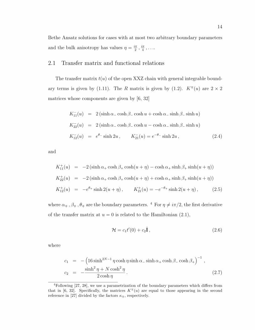
2.1 Transfer matrix and functional relations
The transfer matrix t(u) of the open XXZ chain with general integrable bound-
ary terms is given by (1.11). The R matrix is given by (1.2). K∓(u) are 2 × 2
matrices whose components are given by [6, 32]
K−11(u) = 2 (sinh α− cosh β− cosh u + cosh α− sinh β− sinh u)
K−22(u) = 2 (sinh α− cosh β− cosh u− cosh α− sinh β− sinh u)
K−12(u) = eθ− sinh 2u , K−
21(u) = e−θ− sinh 2u , (2.4)
and
K+11(u) = −2 (sinh α+ cosh β+ cosh(u + η)− cosh α+ sinh β+ sinh(u + η))
K+22(u) = −2 (sinh α+ cosh β+ cosh(u + η) + cosh α+ sinh β+ sinh(u + η))
K+12(u) = −eθ+ sinh 2(u + η) , K+
21(u) = −e−θ+ sinh 2(u + η) , (2.5)
where α∓ , β∓ , θ∓ are the boundary parameters. 4 For η 6= iπ/2, the first derivative
of the transfer matrix at u = 0 is related to the Hamiltonian (2.1),
H = c1t′(0) + c2I , (2.6)
where
c1 = −(16 sinh2N−1 η cosh η sinh α− sinh α+ cosh β− cosh β+
)−1,
c2 = −sinh2 η + N cosh2 η
2 cosh η. (2.7)
4Following [27, 28], we use a parametrization of the boundary parameters which differs fromthat in [6, 32]. Specifically, the matrices K∓(u) are equal to those appearing in the secondreference in [27] divided by the factors κ∓, respectively.

15
and I is the identity matrix. For u = 0, the transfer matrix is given by
t(0) = c0I , c0 = −8 sinh2N η cosh η sinh α− sinh α+ cosh β− cosh β+ . (2.8)
For the special case η = iπ/2 (i.e., p = 1),
t(0) = 0 , t′(0) = d0I , d0 = (−1)N+18i sinh α− sinh α+ cosh β− cosh β+(2.9)
and the Hamiltonian (2.1) is related to the second derivative of the transfer matrix
at u = 0 [25],
H = d1t′′(0) , d1 = (−1)N+1 (32 sinh α− sinh α+ cosh β− cosh β+)−1 . (2.10)
In addition to the fundamental commutativity property
[t(u) , t(v)] = 0 , (2.11)
the transfer matrix also has iπ periodicity
t(u + iπ) = t(u) , (2.12)
crossing symmetry
t(−u− η) = t(u) , (2.13)
and the asymptotic behavior
t(u) ∼ − cosh(θ− − θ+)eu(2N+4)+η(N+2)
22N+1I + . . . for u →∞ . (2.14)
For bulk anisotropy values η = iπp+1
, with p = 1 , 2 , . . ., the transfer matrix
obeys functional relations of order p + 1 [26, 27]
t(u)t(u + η) . . . t(u + pη)
− δ(u− η)t(u + η)t(u + 2η) . . . t(u + (p− 1)η)

16
− δ(u)t(u + 2η)t(u + 3η) . . . t(u + pη)
− δ(u + η)t(u)t(u + 3η)t(u + 4η) . . . t(u + pη)
− δ(u + 2η)t(u)t(u + η)t(u + 4η) . . . t(u + pη)− . . .
− δ(u + (p− 1)η)t(u)t(u + η) . . . t(u + (p− 2)η)
+ . . . = f(u) . (2.15)
For example, for the case p = 2, the functional relation is
t(u)t(u + η)t(u + 2η)− δ(u− η)t(u + η)− δ(u)t(u + 2η) − δ(u + η)t(u)
= f(u) . (2.16)
The functions δ(u) and f(u) are given in terms of the boundary parameters
α∓ , β∓ , θ∓ by
δ(u) = δ0(u)δ1(u) , f(u) = f0(u)f1(u) , (2.17)
where
δ0(u) = (sinh u sinh(u + 2η))2N sinh 2u sinh(2u + 4η)
sinh(2u + η) sinh(2u + 3η), (2.18)
δ1(u) = 24 sinh(u + η + α−) sinh(u + η − α−) cosh(u + η + β−) cosh(u + η − β−)
× sinh(u + η + α+) sinh(u + η − α+) cosh(u + η + β+) cosh(u + η − β+) ,
(2.19)
and therefore,
δ(u + iπ) = δ(u) , δ(−u− 2η) = δ(u) . (2.20)
For p even,
f0(u) = (−1)N+12−2pN sinh2N ((p + 1)u) , (2.21)

17
f1(u) = (−1)N+123−2p(
sinh ((p + 1)α−) cosh ((p + 1)β−) sinh ((p + 1)α+) cosh ((p + 1)β+)
× cosh2 ((p + 1)u)− cosh ((p + 1)α−) sinh ((p + 1)β−) cosh ((p + 1)α+)
× sinh ((p + 1)β+) sinh2 ((p + 1)u)− (−1)N cosh ((p + 1)(θ− − θ+))
× sinh2 ((p + 1)u) cosh2 ((p + 1)u)). (2.22)
For p odd,
f0(u) = (−1)N+12−2pN sinh2N ((p + 1)u) tanh2 ((p + 1)u) , (2.23)
f1(u) = −23−2p(
cosh ((p + 1)α−) cosh ((p + 1)β−) cosh ((p + 1)α+) cosh ((p + 1)β+)
× sinh2 ((p + 1)u)− sinh ((p + 1)α−) sinh ((p + 1)β−) sinh ((p + 1)α+)
× sinh ((p + 1)β+) cosh2 ((p + 1)u) + (−1)N cosh ((p + 1)(θ− − θ+))
× sinh2 ((p + 1)u) cosh2 ((p + 1)u)). (2.24)
Hence, f(u) satisfies
f(u + η) = f(u) , f(−u) = f(u) . (2.25)
We also note the identity
f0(u)2 =p∏
j=0
δ0(u + jη) . (2.26)
The commutativity property (2.11) implies that the eigenvectors |Λ〉 of the
transfer matrix t(u) are independent of the spectral parameter u. Hence, the
corresponding eigenvalues Λ(u) obey the same functional relations (2.15), as well
as the properties (2.12) - (2.14).

18
2.2 Bethe Ansatz solution: Even p, one arbitrary boundary param-eter
We henceforth restrict to even values of p (i.e., bulk anisotropy values η =
iπ3
, iπ5
, . . .), and consider the various special cases that all but one of the boundary
parameters are zero.
2.2.1 α− 6= 0
For the case that all boundary parameters are zero except for α− (or, similarly,
α+), we find that the functional relations (2.15) for the transfer matrix eigenvalues
can be written as
detM = 0 , (2.27)
where M is given by the (p + 1)× (p + 1) matrixΛ(u) −h(u) 0 . . . 0 −h(−u + pη)
−h(−u) Λ(u + pη) −h(u + pη) . . . 0 0...
......
. . ....
...−h(u + p2η) 0 0 . . . −h(−u− p(p− 1)η) Λ(u + p2η)
(2.28)
(whose successive rows are obtained by simultaneously shifting u 7→ u + pη and
cyclically permuting the columns to the right) provided that there exists a function
h(u) which has the properties
h(u + 2iπ) = h (u + 2(p + 1)η) = h(u) , (2.29)
h(u + (p + 2)η) h(−u− (p + 2)η) = δ(u) , (2.30)p∏
j=0
h(u + 2jη) +p∏
j=0
h(−u− 2jη) = f(u) . (2.31)
To solve for h(u), we set
h(u) = h0(u)h1(u) , (2.32)
with
h0(u) = (−1)N sinh2N(u + η)sinh(2u + 2η)
sinh(2u + η). (2.33)

19
Noting that
h0(u + (p + 2)η) h0(−u− (p + 2)η) = δ0(u) ,p∏
j=0
h0(u + 2jη) =p∏
j=0
h0(−u− 2jη) = f0(u) , (2.34)
where δ0(u) and f0(u) are given by (2.18) and (2.21), respectively, we see that
h1(u) must satisfy
h1(u + (p + 2)η) h1(−u− (p + 2)η) = δ1(u) , (2.35)p∏
j=0
h1(u + 2jη) +p∏
j=0
h1(−u− 2jη) = f1(u) . (2.36)
Eliminating h1(−u− 2jη) in (2.36) using (2.35), we obtain
z(u)2 − z(u)f1(u) +p∏
j=0
δ1 (u + (2j − 1)η) = 0 , (2.37)
where
z(u) =p∏
j=0
h1(u + 2jη) . (2.38)
Solving the quadratic equation (2.37) for z(u), making use of the explicit expres-
sions (2.19) and (2.22) for δ1(u) and f1(u), respectively, we obtain
z(u) = 2−2(p−1) cosh2 ((p + 1)u) sinh ((p + 1)u)
× (sinh ((p + 1)u)± sinh ((p + 1)α−)) . (2.39)
Notice that this expression for z(u) has periodicity 2η, which is consistent with
(2.38) and the assumed periodicity (2.29). Corresponding solutions of (2.38) for
h1(u) are
h1(u) = −4 cosh2 u sinh u sinh(u∓ α−)cosh
(12(u± α− + η)
)cosh
(12(u∓ α− − η)
) . (2.40)
In short, a function h(u) which satisfies (2.29) - (2.31) is given by
h(u) = (−1)N+14 sinh2N(u + η)sinh(2u + 2η)
sinh(2u + η)cosh2 u sinh u
× sinh(u− α−)cosh
(12(u + α− + η)
)cosh
(12(u− α− − η)
) . (2.41)

20
The structure of the matrix M (2.28) suggests that its null eigenvector has the
form (Q(u) , Q(u + pη) , . . . , Q(u + p2η)), where Q(u) has the periodicity property
Q(u + 2iπ) = Q(u) . (2.42)
It follows that the transfer matrix eigenvalues are given by
Λ(u) = h(u)Q(u + pη)
Q(u)+ h(−u + pη)
Q(u− pη)
Q(u), (2.43)
which evidently has the form of Baxter’s TQ relation. We make the Ansatz
Q(u) =M∏
j=1
sinh(
1
2(u− uj)
)sinh
(1
2(u + uj − pη)
), (2.44)
which has the periodicity (2.42) as well as the crossing property 5
Q(−u + pη) = Q(u) . (2.45)
The asymptotic behavior (2.14) is consistent with having M (the number of zeros
uj of Q(u)) given by
M = N + p + 1 , (2.46)
which we have confirmed numerically for small values of N and p. Analyticity of
Λ(u) implies the Bethe Ansatz equations
h(uj)
h(−uj + pη)= −Q(uj − pη)
Q(uj + pη), j = 1 , . . . , M . (2.47)
To summarize, for the special case that p is even and all boundary parameters
are zero except for α−, the eigenvalues of the transfer matrix (1.11) are given by
(2.43), where h(u) is given by (2.41), and Q(u) is given by (2.44) and (2.46), with
zeros uj given by (2.47).
5Note that Λ(u) = Λ(−u + pη) = Λ(−u− η), where the first equality follows from (2.43) and(2.45), and the second equality follows from the iπ periodicity of Λ(u) (which, however, is notmanifest from (2.43).)

21
We observe that for the special case that we are considering, the corresponding
Hamiltonian is not of the usual XXZ form. Indeed, t′(0) (the first derivative of
the transfer matrix evaluated at u = 0) is proportional to σxN . Hence, to obtain a
nontrivial integrable Hamiltonian, one must consider the second derivative of the
transfer matrix. We find
t′′(0) = −16 sinh2N−1 η cosh η sinh α−
({σx
N ,N−1∑n=1
Hn ,n+1
}
+ (N cosh η + sinh η tanh η)σxN +
sinh η
sinh α−σx
1σxN
), (2.48)
where Hn ,n+1 is given by
Hn ,n+1 =1
2
(σx
nσxn+1 + σy
nσyn+1 + cosh η σz
nσzn+1
). (2.49)
2.2.2 β− 6= 0
For the case that all boundary parameters are zero except for β− (or, similarly,
β+), we find that the functional relations (2.15) for the transfer matrix eigenvalues
can again be written in the form (2.27), where now the matrix M is given by
Λ(u) −h(u) 0 . . . 0 −h(−u− η)
−h(−u− (p + 1)η) Λ(u + pη) −h(u + pη) . . . 0 0...
......
. . ....
...−h(u + p2η) 0 0 . . . −h(−u− (p2 + 1)η) Λ(u + p2η)
(2.50)
if h(u) satisfies
h(u + 2iπ) = h (u + 2(p + 1)η) = h(u) , (2.51)
h(u + (p + 2)η) h(−u− η) = δ(u) , (2.52)p∏
j=0
h(u + 2jη) +p∏
j=0
h(−u− (2j + 1)η) = f(u) . (2.53)
Proceeding similarly to the previous case, we now find
h(u) = (−1)N4 sinh2N(u + η)sinh(2u + 2η)
sinh(2u + η)sinh2 u cosh u
×(cosh u + (−1)
p2 i sinh β−
). (2.54)

22
The transfer matrix eigenvalues are now given by
Λ(u) = h(u)Q(u + pη)
Q(u)+ h(−u− η)
Q(u− pη)
Q(u), (2.55)
with
Q(u) =M∏
j=1
sinh(
1
2(u− uj)
)sinh
(1
2(u + uj + η)
), (2.56)
which satisfies Q(u + 2iπ) = Q(u) and Q(−u− η) = Q(u); and
M = N + p . (2.57)
Moreover, the Bethe Ansatz equations for the zeros uj take the form
h(uj)
h(−uj − η)= −Q(uj − pη)
Q(uj + pη), j = 1 , . . . , M . (2.58)
For this case, t′(0) = 0, and
t′′(0) = −16 cosh η sinh2N η (σx1 + sinh β− σz
1) σxN . (2.59)
Higher derivatives yield more complicated expressions.
2.2.3 θ∓ 6= 0
For the case that all boundary parameters are zero except for θ− and θ+ (quan-
tities of interest depend only on the difference θ−−θ+), we find that the functional
relations (2.15) for the transfer matrix eigenvalues can be written in the form
(2.27), where the matrix M is given by
Λ(u) −h(2)(−u− η) 0 . . . 0 −h(1)(u)
−h(1)(u + η) Λ(u + η) −h(2)(−u− 2η) . . . 0 0...
......
. . ....
...−h(2)(−u− (p + 1)η) 0 0 . . . −h(1)(u + pη) Λ(u + pη)
(2.60)
(whose successive rows are obtained by simultaneously shifting u 7→ u + η and
cyclically permuting the columns to the right), if the functions h(1)(u) and h(2)(u)

23
satisfy
h(k)(u + iπ) = h(k) (u + (p + 1)η) = h(k)(u) , k = 1 , 2 , (2.61)
h(1)(u + η) h(2)(−u− η) = δ(u) , (2.62)p∏
j=0
h(1)(u + jη) +p∏
j=0
h(2)(−u− jη) = f(u) . (2.63)
We find
h(1)(u) = (−1)Neθ+−θ− sinh2N(u + η)sinh(2u + 2η)
sinh(2u + η)sinh2 2u ,
h(2)(u) = (−1)Neθ−−θ+ sinh2N(u + η)sinh(2u + 2η)
sinh(2u + η)sinh2 2u . (2.64)
The transfer matrix eigenvalues are given by
Λ(u) = h(1)(u)Q(u− η)
Q(u)+ h(2)(−u− η)
Q(u + η)
Q(u), (2.65)
with, for N even,
Q(u) =2M∏j=1
sinh(u− uj) , (2.66)
which satisfies Q(u + iπ) = Q(u); and
M =1
2(N + p) . (2.67)
The Bethe Ansatz equations for the zeros uj take the form
h(1)(uj)
h(2)(−uj − η)= −Q(uj + η)
Q(uj − η), j = 1 , . . . , M . (2.68)
For this case, also t′(0) = 0, and
t′′(0) = −16 cosh η sinh2N η(
cosh θ− cosh θ+ σx1σx
N + i cosh θ− sinh θ+ σx1σy
N
+ i sinh θ− cosh θ+ σy1σ
xN − sinh θ− sinh θ+ σy
1σyN
). (2.69)
24
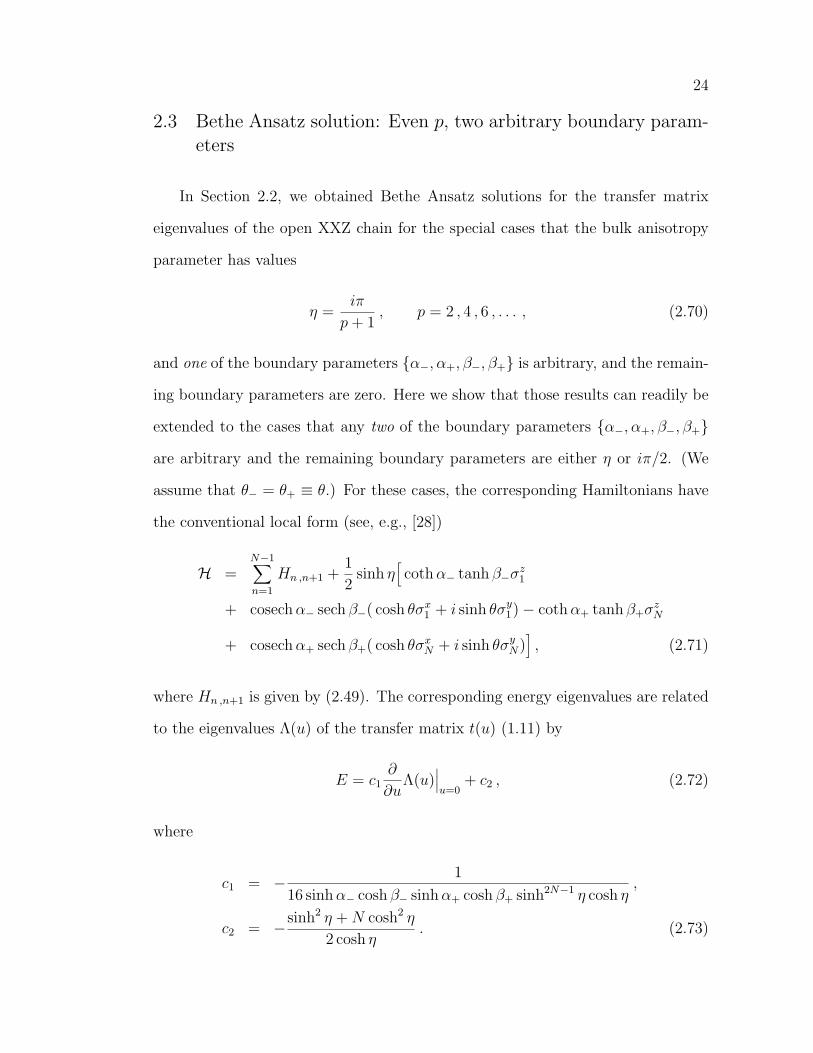
2.3 Bethe Ansatz solution: Even p, two arbitrary boundary param-eters
In Section 2.2, we obtained Bethe Ansatz solutions for the transfer matrix
eigenvalues of the open XXZ chain for the special cases that the bulk anisotropy
parameter has values
η =iπ
p + 1, p = 2 , 4 , 6 , . . . , (2.70)
and one of the boundary parameters {α−, α+, β−, β+} is arbitrary, and the remain-
ing boundary parameters are zero. Here we show that those results can readily be
extended to the cases that any two of the boundary parameters {α−, α+, β−, β+}
are arbitrary and the remaining boundary parameters are either η or iπ/2. (We
assume that θ− = θ+ ≡ θ.) For these cases, the corresponding Hamiltonians have
the conventional local form (see, e.g., [28])
H =N−1∑n=1
Hn ,n+1 +1
2sinh η
[coth α− tanh β−σz
1
+ cosech α− sech β−( cosh θσx1 + i sinh θσy
1)− coth α+ tanh β+σzN
+ cosech α+ sech β+( cosh θσxN + i sinh θσy
N)], (2.71)
where Hn ,n+1 is given by (2.49). The corresponding energy eigenvalues are related
to the eigenvalues Λ(u) of the transfer matrix t(u) (1.11) by
E = c1∂
∂uΛ(u)
∣∣∣u=0
+ c2 , (2.72)
where
c1 = − 1
16 sinh α− cosh β− sinh α+ cosh β+ sinh2N−1 η cosh η,
c2 = −sinh2 η + N cosh2 η
2 cosh η. (2.73)

25
2.3.1 α− , α+ arbitrary
For the case that α± are arbitrary and β± = η, we find that√√√√f1(u)2 − 4p∏
j=0
δ1 (u + (2j − 1)η) = 2−2p+3 cosh2 ((p + 1)u) sinh ((p + 1)u)
×[sinh ((p + 1)α−)− (−1)N sinh ((p + 1)α+)
].
(2.74)
The key point is that the argument of the square root is a perfect square. For
definiteness, we henceforth restrict to even values of N . It follows that the quantity
z(u) appearing in (2.37) is now given by (cf. (2.39))
z(u) = 2−2(p−1) cosh2 ((p + 1)u) [sinh ((p + 1)u)± sinh ((p + 1)α−)]
× [sinh ((p + 1)u)∓ sinh ((p + 1)α+)] . (2.75)
Corresponding solutions of (2.38) for h1(u) are (cf. (2.40))
h1(u) = 4 cosh2(u− η) sinh(u∓ α−) sinh(u± α+)
×cosh
(12(u± α− + η)
)cosh
(12(u∓ α− − η)
) cosh(
12(u∓ α+ + η)
)cosh
(12(u± α+ − η)
) . (2.76)
Hence, for h(u) = h0(u)h1(u) we can take (cf. (2.41))
h(u) = 4 sinh2N(u + η)sinh(2u + 2η)
sinh(2u + η)cosh2(u− η)
× sinh(u− α−) sinh(u + α+)cosh
(12(u + α− + η)
)cosh
(12(u− α− − η)
) cosh(
12(u− α+ + η)
)cosh
(12(u + α+ − η)
) ,
(2.77)
which indeed satisfies (2.29)-(2.31). The transfer matrix eigenvalues and Bethe
Ansatz equations are given by (2.43), (2.44), (2.47), with (cf. (2.46))
M = N + 2p + 1 . (2.78)

26
2.3.2 β− , β+ arbitrary
For the case that β± are arbitrary and α± = η, we find that√√√√f1(u)2 − 4p∏
j=0
δ1 (u + (2j − 1)η) = i2−2p+3 sinh2 ((p + 1)u) cosh ((p + 1)u)
× [sinh ((p + 1)β−)− sinh ((p + 1)β+)]
(2.79)
and therefore
z(u) = 2−2(p−1) sinh2 ((p + 1)u) [cosh ((p + 1)u)± i sinh ((p + 1)β−)]
× [cosh ((p + 1)u)∓ i sinh ((p + 1)β+)] . (2.80)
Thus, we take the function h(u) to be (cf. (2.54))
h(u) = 4 sinh2N(u + η)sinh(2u + 2η)
sinh(2u + η)sinh2(u− η)
× (cosh u + i sinh β−) (cosh u− i sinh β+) , (2.81)
which indeed satisfies (2.51)-(2.53). The transfer matrix eigenvalues and Bethe
Ansatz equations are given by (2.55), (2.56), (2.58), with (cf. (2.57))
M = N + 2p− 1 . (2.82)
2.3.3 α− , β− arbitrary
For the case that α− , β− are arbitrary and α+ = iπ/2, β+ = η, we find that√√√√f1(u)2 − 4p∏
j=0
δ1 (u + (2j − 1)η) = 2−2p+3 cosh2 ((p + 1)u) sinh ((p + 1)u)
×[sinh ((p + 1)α−) + (−1)
p2 i cosh ((p + 1)β−)
],
(2.83)
and therefore
z(u) = 2−2(p−1) cosh2 ((p + 1)u) [sinh ((p + 1)u)± sinh ((p + 1)α−)]
×[sinh ((p + 1)u)± (−1)
p2 i cosh ((p + 1)β−)
]. (2.84)

27
For h(u) we take
h(u) = 4 sinh2N(u + η)sinh(2u + 2η)
sinh(2u + η)cosh(u− η) cosh u
× sinh(u− α−)cosh
(12(u + α− + η)
)cosh
(12(u− α− − η)
) (sinh u + i cosh β−) , (2.85)
which satisfies (2.29)-(2.31). The transfer matrix eigenvalues and Bethe Ansatz
equations are given by (2.43), (2.44), (2.47), with (cf. (2.46))
M = N + p . (2.86)
Similar results hold for the case that α+ , β+ are arbitrary and α− = iπ/2, β− = η,
etc.
We have checked these solutions numerically for chains of length up to N =
6, and have verified that they give the complete set of 2N eigenvalues. Hence,
completeness is achieved more simply than in the case that the constraint (2.3) is
satisfied [28].
We emphasize that, in contrast to the solution for the case that the con-
straint (2.3) is satisfied, these solutions do not hold for generic values of the bulk
anisotropy. Indeed, these solutions hold only for η = iπ3
, iπ5
, . . .. Also, while the
Q(u) functions have periodicity iπ for the case that the constraint (2.3) is satisfied
and for the case treated in Section 2.2.3, the Q(u) functions have only 2iπ period-
icity for the cases treated in Sections 2.2.1 and 2.2.2. (See Eqs. (A1.10), (2.66),
(2.44) and (2.56), respectively.)
Two key steps in our approach for solving for the function h(u) (which permits
the recasting of the functional relations (2.15) as the vanishing of a determinant
(2.27)) are solving the quadratic equation (2.37) for z(u), and factoring the result,
such as in (2.38). For the special cases solved so far (namely, the case (2.3) consid-
ered in [24, 27, 28], and the new cases considered here), the discriminants of the

28
corresponding quadratic equations are perfect squares, and the factorizations can
be readily carried out. However, for general values of the boundary parameters,
the discriminant is no longer a perfect square; and factoring the result becomes a
formidable challenge. Perhaps elliptic functions may prove useful in this regard. 6
2.4 Bethe Ansatz solution: Odd p, two arbitrary boundary param-eters
The famous Baxter T −Q relation [35], which schematically has the form
t(u) Q(u) = Q(u′) + Q(u′′) , (2.87)
holds for many integrable models associated with the sl2 Lie algebra and its defor-
mations, such as the closed XXZ quantum spin chain. This relation provides one
of the most direct routes to the Bethe Ansatz expression for the eigenvalues of the
transfer matrix t(u).
We present a generalization of this relation which involves more than one Q(u),
t(u) Q1(u) = Q2(u′) + Q2(u
′′) ,
t(u) Q2(u) = Q1(u′′′) + Q1(u
′′′′) . (2.88)
This structure arises naturally in the open XXZ quantum spin chain for special
values of the bulk and boundary parameters. We expect that such generalized
T − Q relations, involving two or more independent Q(u)’s, may also appear in
other integrable models.
We find here (again by means of the functional relations approach) that by
allowing the possibility of generalized T−Q relations, we can obtain Bethe-Ansatz-
type expressions for the transfer matrix eigenvalues for the cases that at most two
of the boundary parameters {α−, α+, β−, β+} are nonzero, and the bulk anisotropy
6An attempt along this line for the case p = 1 was considered in [25].

29
has values η = iπ2
, iπ4
, . . .. In order to derive the generalized T − Q relation, it is
instructive to first understand why we are unable to obtain a conventional relation
with a single Q(u).
2.5 An attempt to obtain a conventional T −Q relation
In order to obtain Bethe Ansatz expressions for the transfer matrix eigenvalues,
we try (following [38]) to recast the functional relations as the condition that the
determinant of a certain matrix vanishes. To this end, let us consider again the
(p + 1)× (p + 1) matrix given by [27]
M(u) =
Λ(u) − δ(u)
h(u+η)0 . . . 0 −h(u)
−h(u + η) Λ(u + η) − δ(u+η)h(u+2η)
. . . 0 0...
......
. . ....
...
− δ(u−η)h(u)
0 0 . . . −h(u + pη) Λ(u + pη)
(2.89)
where h(u) is a function which is iπ-periodic, but otherwise not yet specified.
Evidently, successive rows of this matrix are obtained by simultaneously shifting
u 7→ u + η and cyclically permuting the columns to the right. Hence, this matrix
has the symmetry property
SM(u)S−1 = M(u + η) , (2.90)
where S is the (p + 1)× (p + 1) matrix given by
S =
0 1 0 . . . 0 00 0 1 . . . 0 0...
......
. . ....
...0 0 0 . . . 0 11 0 0 . . . 0 0
, Sp+1 = 1 . (2.91)
This symmetry implies that the corresponding T − Q relation would involve
only one Q(u). Indeed, if we assume detM(u) = 0 (which, as we discuss below,
turns out to be false for the cases which we consider here), then M(u) has a null
30
eigenvector,
M(u) v(u) = 0 . (2.92)
The symmetry (2.90) is consistent with
S v(u) = v(u + η) , (2.93)
which in turn implies that v(u) has the form
v(u) = (Q(u) , Q(u + η) , . . . , Q(u + pη)) , Q(u + iπ) = Q(u) . (2.94)
That is, all the components of v(u) are determined by a single function Q(u). The
null eigenvector condition (2.92) together with the explicit forms (2.89), (2.94) of
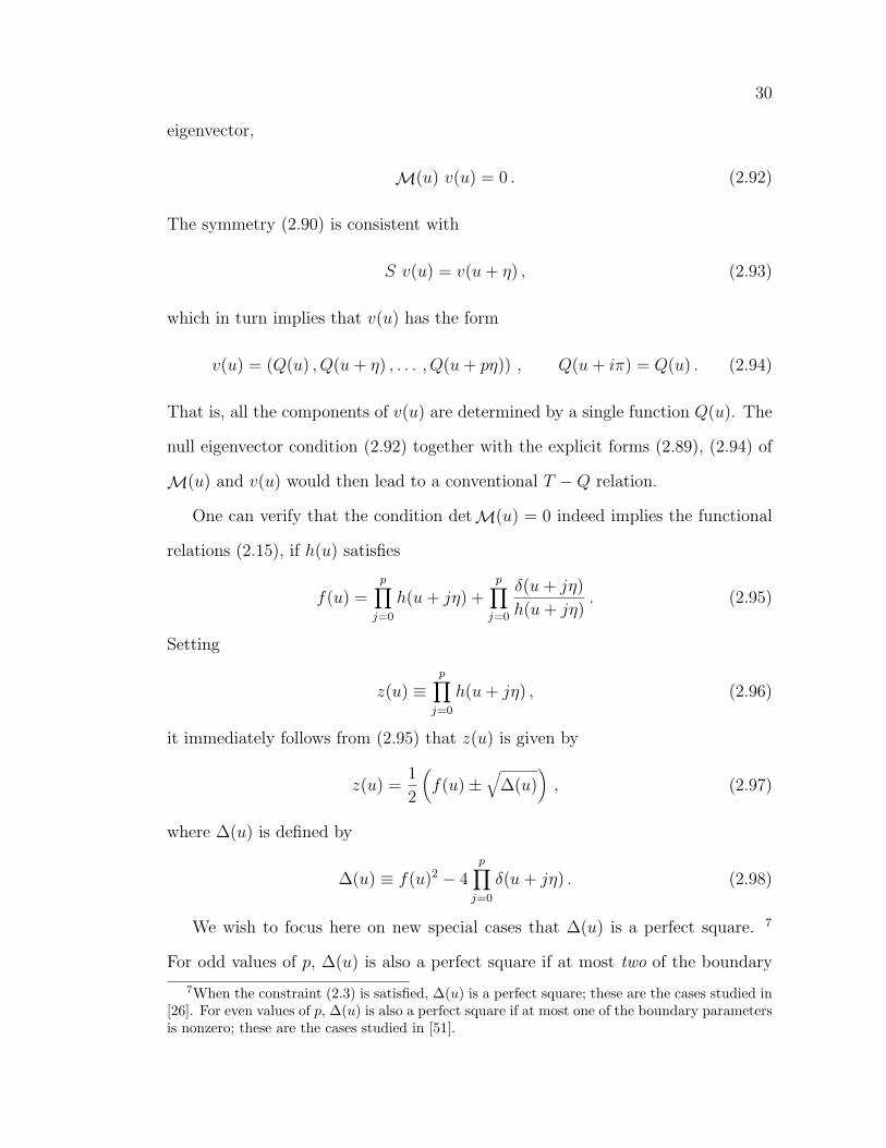
M(u) and v(u) would then lead to a conventional T −Q relation.
One can verify that the condition detM(u) = 0 indeed implies the functional
relations (2.15), if h(u) satisfies
f(u) =p∏
j=0
h(u + jη) +p∏
j=0
δ(u + jη)
h(u + jη). (2.95)
Setting
z(u) ≡p∏
j=0
h(u + jη) , (2.96)
it immediately follows from (2.95) that z(u) is given by
z(u) =1
2
(f(u)±
√∆(u)
), (2.97)
where ∆(u) is defined by
∆(u) ≡ f(u)2 − 4p∏
j=0
δ(u + jη) . (2.98)
We wish to focus here on new special cases that ∆(u) is a perfect square. 7
For odd values of p, ∆(u) is also a perfect square if at most two of the boundary
7When the constraint (2.3) is satisfied, ∆(u) is a perfect square; these are the cases studied in[26]. For even values of p, ∆(u) is also a perfect square if at most one of the boundary parametersis nonzero; these are the cases studied in [51].
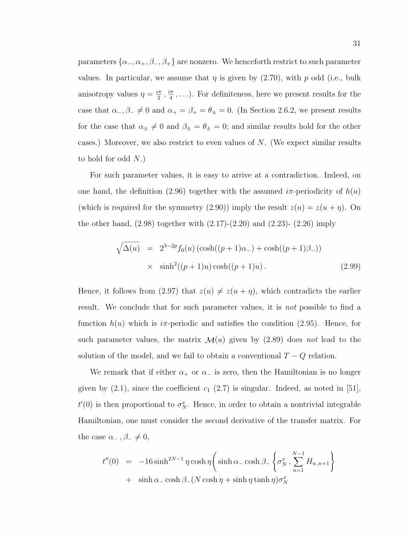
31
parameters {α−, α+, β−, β+} are nonzero. We henceforth restrict to such parameter
values. In particular, we assume that η is given by (2.70), with p odd (i.e., bulk
anisotropy values η = iπ2
, iπ4
, . . .). For definiteness, here we present results for the
case that α−, β− 6= 0 and α+ = β+ = θ± = 0. (In Section 2.6.2, we present results
for the case that α± 6= 0 and β± = θ± = 0; and similar results hold for the other
cases.) Moreover, we also restrict to even values of N . (We expect similar results
to hold for odd N .)
For such parameter values, it is easy to arrive at a contradiction. Indeed, on
one hand, the definition (2.96) together with the assumed iπ-periodicity of h(u)
(which is required for the symmetry (2.90)) imply the result z(u) = z(u + η). On
the other hand, (2.98) together with (2.17)-(2.20) and (2.23)- (2.26) imply
√∆(u) = 23−2pf0(u) (cosh((p + 1)α−) + cosh((p + 1)β−))
× sinh2((p + 1)u) cosh((p + 1)u) . (2.99)
Hence, it follows from (2.97) that z(u) 6= z(u + η), which contradicts the earlier
result. We conclude that for such parameter values, it is not possible to find a
function h(u) which is iπ-periodic and satisfies the condition (2.95). Hence, for
such parameter values, the matrix M(u) given by (2.89) does not lead to the
solution of the model, and we fail to obtain a conventional T −Q relation.
We remark that if either α+ or α− is zero, then the Hamiltonian is no longer
given by (2.1), since the coefficient c1 (2.7) is singular. Indeed, as noted in [51],
t′(0) is then proportional to σxN . Hence, in order to obtain a nontrivial integrable
Hamiltonian, one must consider the second derivative of the transfer matrix. For
the case α− , β− 6= 0,
t′′(0) = −16 sinh2N−1 η cosh η
(sinh α− cosh β−
{σx
N ,N−1∑n=1
Hn ,n+1
}+ sinh α− cosh β−(N cosh η + sinh η tanh η)σx
N

32
+ sinh η (σx1 + sinh β− cosh α−σz
1) σxN
), (2.100)
where Hn ,n+1 is given by (2.49). The case α± 6= 0, for which the Hamiltonian
instead has a conventional local form, will be discussed in the following section.
2.6 The generalized T −Q relations
Instead of demanding the symmetry (2.90), let us now demand only the weaker
symmetry
T M(u)T−1 = M(u + 2η) , T ≡ S2 , (2.101)
where S is given by (2.91). Indeed, (2.90) implies (2.101), but the converse is not
true. A matrix M(u) with such symmetry is given by
Λ(u) − δ(u)
h(1)(u)0 . . . 0 − δ(u−η)
h(2)(u−η)
−h(1)(u) Λ(u + η) −h(2)(u + η) . . . 0 0...
......
. . ....
...−h(2)(u− η) 0 0 . . . −h(1)(u + (p− 1)η) Λ(u + pη)
(2.102)
where h(1)(u) and h(2)(u) are functions which are iπ-periodic, but otherwise not
yet specified.
This symmetry implies that the corresponding T −Q relations will involve two
Q(u)’s. Indeed, assuming again that
detM(u) = 0 , (2.103)
then M(u) has a null eigenvector v(u),
M(u) v(u) = 0 . (2.104)
The symmetry (2.101) is consistent with
T v(u) = v(u + 2η) , (2.105)

33
which implies that v(u) has the form
v(u) = (Q1(u) , Q2(u) , . . . , Q1(u− 2η) , Q2(u− 2η)) , (2.106)
with
Q1(u) = Q1(u + iπ) , Q2(u) = Q2(u + iπ) . (2.107)
That is, the components of v(u) are determined by two independent functions,
Q1(u) and Q2(u). The null eigenvector condition (2.104) together with the explicit
forms (2.102), (2.106) of M(u) and v(u) now lead to generalized T −Q relations,
Λ(u) =δ(u)
h(1)(u)
Q2(u)
Q1(u)+
δ(u− η)
h(2)(u− η)
Q2(u− 2η)
Q1(u), (2.108)
= h(1)(u− η)Q1(u− η)
Q2(u− η)+ h(2)(u)
Q1(u + η)
Q2(u− η). (2.109)
Since Λ(u) has the crossing symmetry (2.13) and δ(u) has the crossing property
(2.20), it is natural to have the two terms in (2.108) transform into each other under
crossing. Hence, we set
h(2)(u) = h(1)(−u− 2η) , (2.110)
and we make the Ansatz
Q1(u) =M1∏j=1
sinh(u− u(1)j ) sinh(u + u
(1)j + η) ,
Q2(u) =M2∏j=1
sinh(u− u(2)j ) sinh(u + u
(2)j + 3η) , (2.111)
which is consistent with the required periodicity (2.107) and crossing properties
Q1(u) = Q1(−u− η) , Q2(u) = Q2(−u− 3η) . (2.112)
Analyticity of Λ(u) (2.108), (2.109) implies Bethe-Ansatz-type equations for
the zeros {u(1)j , u
(2)j } of Q1(u) , Q2(u), respectively,
δ(u(1)j ) h(2)(u
(1)j − η)
δ(u(1)j − η) h(1)(u
(1)j )
= −Q2(u
(1)j − 2η)
Q2(u(1)j )
, j = 1 , 2 , . . . , M1 ,
h(1)(u(2)j )
h(2)(u(2)j + η)
= −Q1(u
(2)j + 2η)
Q1(u(2)j )
, j = 1 , 2 , . . . , M2 . (2.113)

34
Note that the function h(1)(u) has not yet been specified, nor has the impor-
tant assumption that M(u) has a vanishing determinant (2.103) yet been verified.
These problems are closely related, and we now address them both.
One can verify that the condition detM(u) = 0 indeed implies the functional
relations (2.15), if h(1)(u) satisfies
f(u) = w(u)p−1∏
j=0,2,...
δ(u + jη) +1
w(u)
p∏j=1,3,...
δ(u + jη) , (2.114)
where
w(u) ≡∏p
j=1,3,... h(2)(u + jη)∏p−1
j=0,2,... h(1)(u + jη)
. (2.115)
It immediately follows from (2.114) that w(u) is given by
w(u) =f(u)±
√∆(u)
2∏p−1
j=0,2,... δ(u + jη), (2.116)
where ∆(u) is the same quantity defined in (2.98).
2.6.1 α− 6= 0, β− 6= 0 and α+ = β+ = θ± = 0
We consider the case that p is odd, and that at most α− and β− are nonzero. For
this case,√
∆(u) is given by (2.99). It follows from (2.116) that for p = 3 , 7 , 11 , . . .
the two solutions for w(u) are given by
w(u) = coth2N(
1
2(p + 1)u
),
w(u) =
(cosh((p + 1)u)− cosh((p + 1)α−)
cosh((p + 1)u) + cosh((p + 1)α−)
)(cosh((p + 1)u)− cosh((p + 1)β−)
cosh((p + 1)u) + cosh((p + 1)β−)
)
× coth2N(
1
2(p + 1)u
), p = 3 , 7 , 11 , . . . ; (2.117)
and for p = 1 , 5 , 9 , . . . the two solutions for w(u) are given by
w(u) =
(cosh((p + 1)u)− cosh((p + 1)α−)
cosh((p + 1)u) + cosh((p + 1)α−)
)coth2N
(1
2(p + 1)u
),
w(u) =
(cosh((p + 1)u) + cosh((p + 1)β−)
cosh((p + 1)u)− cosh((p + 1)β−)
)coth2N
(1
2(p + 1)u
),
p = 1 , 5 , 9 , . . . . (2.118)

35
There are many solutions of (2.115) for h(1)(u) (with h(2)(u) given by (2.110))
corresponding to the above expressions for w(u), which also have the required iπ
periodicity. We consider here the solutions
h(1)(u) = −4 sinh2N(u + 2η) , M2 =1
2N + p− 1 , M1 = M2 + 2 ,
p = 3 , 7 , 11 , . . . (2.119)
and
h(1)(u) =
−2 cosh(u + α−) cosh(u− α−) cosh(2u) sinh2N(u + 2η) ,M1 = M2 = 1
2N + 2p− 1 , p = 9 , 17 , 25 , . . .
2 cosh(u + α−) cosh(u− α−) cosh(2u) sinh2N(u + 2η) ,M1 = M2 = 1
2N + 3
2(p− 1) , p = 5 , 13 , 21 , . . .
2 cosh(u + α−) cosh(u− α−) cosh(2u) sinh2N(u + 2η) ,M1 = M2 = 1
2N + 2 , p = 1 ,
(2.120)
corresponding to the first solutions for w(u) given in (2.117), (2.118), respectively.
We have searched for solutions largely by trial and error, verifying numerically
(along the lines explained in [28]) for small values of N that the eigenvalues can
indeed be expressed as (2.108), (2.109) with Q(u)’s of the form (2.111).
Note that the values of M1 and M2 (i.e., the number of zeros of Q1(u) and
Q2(u), respectively) depend on the particular choice for the function h(1)(u). Our
reason for choosing (2.119), (2.120) over the other solutions which we found is that
the former solutions gave the lowest values of M1 and M2, for given values of N
and p. (It would be interesting to know whether there exist other solutions for
h(1)(u) which give even lower values of M1 and M2.) Our conjectured values of
M1 and M2 given in (2.119), (2.120) are consistent with the asymptotic behavior
(2.14). Moreover, these values have been checked numerically for small values of
N (up to N = 6) and p (up to p = 21). That is, we have verified numerically that,
with the above choice of h(1)(u), the generalized T − Q relations (2.108), (2.109)
correctly give all 2N eigenvalues, with Q1(u) and Q2(u) of the form (2.111) and
36
with M1 and M2 given in (2.119), (2.120). We expect that similar results can be
obtained corresponding to the second solutions for w(u).
We propose that for the case that p is odd and that at most α−, β− are nonzero,
the eigenvalues Λ(u) of the transfer matrix t(u) (1.11) are given by the generalized
T − Q relations (2.108), (2.109), with Q1(u) and Q2(u) given by (2.111), h(2)(u)
given by (2.110), and h(1)(u) given by (2.119), (2.120). The zeros {u(1)j , u
(2)j }
of Q1(u) and Q2(u) are solutions of the Bethe Ansatz equations (2.113). We
expect that there are sufficiently many such equations to determine all the zeros.
As already mentioned, similar results hold for the case that at most two of the
boundary parameters {α−, α+, β−, β+} are nonzero.
2.6.2 α± 6= 0 and β± = θ± = 0
Here we consider the case that α± 6= 0 and β± = θ± = 0, for which the
Hamiltonian is local,
H =N−1∑n=1
Hn ,n+1 +1
2sinh η
(cosech α−σx
1 + cosech α+σxN
), (2.121)
as follows from (2.1). For this case, the quantity√
∆(u) is given by (2.99) with β−
replaced by α+, namely,
√∆(u) = 23−2pf0(u) (cosh((p + 1)α−) + cosh((p + 1)α+))
× sinh2((p + 1)u) cosh((p + 1)u) . (2.122)
It follows that the two solutions for w(u) (2.116) are given by
w(u) = coth2N(
1
2(p + 1)u
),
w(u) =
(cosh((p + 1)u)− cosh((p + 1)α−)
cosh((p + 1)u) + cosh((p + 1)α−)
)(cosh((p + 1)u)− cosh((p + 1)α+)
cosh((p + 1)u) + cosh((p + 1)α+)
)
× coth2N(
1
2(p + 1)u
), p = 3 , 7 , 11 , . . . , (2.123)

37
and
w(u) = coth2N+2(
1
2(p + 1)u
),
w(u) =
(cosh((p + 1)u)− cosh((p + 1)α−)
cosh((p + 1)u) + cosh((p + 1)α−)
)(cosh((p + 1)u)− cosh((p + 1)α+)
cosh((p + 1)u) + cosh((p + 1)α+)
)
× coth2N+2(
1
2(p + 1)u
), p = 1 , 5 , 9 , . . . . (2.124)
For simplicity, let us once again consider just the first solutions for w(u) given
in (2.123) and (2.124), which are independent of α±. Corresponding solutions of
(2.115) for h(1)(u) (with h(2)(u) given by (2.110)) are
h(1)(u) = 4 sinh2N(u + 2η) , M2 =1
2N +
1
2(3p− 1) , M1 = M2 + 2 ,
p = 3 , 7 , 11 , . . . (2.125)
and
h(1)(u) =
−2 cosh(2u) sinh2 u sinh2N(u + 2η) , M1 = M2 = 12N + 2p− 1 ,
p = 9 , 17 , 25 , . . .2 cosh(2u) sinh2 u sinh2N(u + 2η) , M1 = M2 = 1
2N + 3
2(p− 1) ,
p = 5 , 13 , 21 , . . .2 cosh(2u) sinh2 u sinh2N(u + 2η) , M1 = M2 = 1
2N + 2 ,
p = 1 .
(2.126)
That is, the eigenvalues Λ(u) of the transfer matrix t(u) (1.11), for η values (2.70)
with p odd and for α± 6= 0 and β± = θ± = 0, are given by the generalized T −Q
relations (2.108), (2.109), with Q1(u) and Q2(u) given by (2.111), h(2)(u) given by
(2.110), and h(1)(u) given by (2.125), (2.126). The zeros {u(1)j , u
(2)j } of Q1(u) and
Q2(u) are solutions of the Bethe Ansatz equations (2.113).
We have argued that the eigenvalues of the transfer matrix of the open XXZ
chain, for the special case that p is odd and that at most two of the boundary
parameters {α−, α+, β−, β+} are nonzero, can be given by generalized T −Q rela-
tions (2.108), (2.109) involving more than one Q(u). Although we have not ruled
out the possibility of expressing these eigenvalues in terms of a conventional T −Q
relation, the analysis in Section 2.5 suggests to us that this is unlikely.

38
It should be possible to explicitly construct operators Q1(u), Q2(u) which com-
mute with each other and with the transfer matrix t(u), and whose eigenvalues
are given by (2.111). There may be further special cases for which the quantity
∆(u) (2.98) is a perfect square, in which case it should not be difficult to find the
corresponding Bethe Ansatz solution. The general case that ∆(u) is not a perfect
square and/or that η 6= iπ/(p + 1) remains to be understood.
Generalized T −Q relations are novel structures, which merit further investiga-
tion. The corresponding Bethe Ansatz equations (e.g., (2.113)) have some resem-
blance to the “nested” equations which are characteristic of higher-rank models.
Such generalized T − Q relations, involving two or even more Q(u)’s, may also
lead to further solutions of integrable open chains of higher rank and/or higher-
dimensional representations. (For recent progress on such models, see e.g. [44].)

Chapter 3: Bethe Ansatz For General Case of anOpen XXZ Spin Chain
There remains the vexing problem of solving the model when the constraint (2.3)
is not satisfied, i.e., for arbitrary values of the boundary parameters. Our goal has
been to solve this problem for the root of unity case. Some progress was already
achieved in [51, 52], where Bethe-Ansatz-type solutions for special cases with up
to two free boundary parameters (and with the remaining boundary parameters
fixed to specific values) were proposed. For those special cases (as well as for the
cases where the constraint (2.3) is satisfied), the quantity ∆(u) defined by (2.98),
namely
∆(u) = f(u)2 − 4p∏
j=0
δ(u + jη) (3.1)
is a perfect square. However, for generic values of boundary parameters, ∆(u) is
not a perfect square, and it had not been clear to us how to proceed. It is on this
generic case that we focus in this chapter.
We find, for generic values of the boundary parameters, expressions for the
eigenvalues Λ(u) of the transfer matrix t(u) in terms of sets of “Q functions”
{ai(u) , bi(u)}, whose zeros are given by Bethe-Ansatz-like equations. (See (3.42),
(3.43) for p > 1; and (3.69), (3.70) for p = 1.) Such generalized T − Q relations,
involving more than one Q function, appeared already for certain special cases
[52], and were used in [53] to compute the corresponding boundary energies in
the thermodynamic limit. We have verified the T − Q relations numerically for
small values of p and N , and confirmed that they describe the complete set of 2N
eigenvalues.
39

40
3.1 The case p > 1
We treat in this section the case η = iπ/(p+1) with p > 1, i.e., bulk anisotropy
values η = iπ3
, iπ4
, . . .. Following Bazhanov and Reshetikhin [38], we first recast the
functional relations for the transfer matrix eigenvalues Λ(u) as the condition that
a matrix M(u) have zero determinant. The equations for the corresponding null
eigenvector, together with a key Ansatz (3.38)-(3.39), then lead to the desired set of
generalized T−Q relations for Λ(u) (3.42), (3.43) and the associated Bethe-Ansatz
equations (3.45)-(3.52).
3.1.1 The matrix M(u)
Our objective is to determine the eigenvalues Λ(u) of the transfer matrix t(u).
As noted earlier, the transfer matrix satisfies a functional relation (2.15). By virtue
of the commutativity property (2.11), the eigenvalues satisfy the same functional
relation as the corresponding transfer matrix, as well as the properties (2.12) -
(2.14). Hence, for example, for p = 2 the eigenvalues satisfy
Λ(u) Λ(u + η) Λ(u + 2η) − δ(u) Λ(u + 2η)− δ(u + η) Λ(u)
− δ(u + 2η) Λ(u + η) = f(u) . (3.2)
The first main step is to reformulate the functional relation as the condition
that the determinant of some matrix vanish. To this end, let us consider the
(p + 1)× (p + 1) matrix M(u) given by
Λ(u) −m1(u) 0 . . . 0 0 −np+1(u)−n1(u) Λ(u + η) −m2(u) . . . 0 0 0
......
.... . .
......
...0 0 0 . . . −np−1(u) Λ(u + (p− 1)η) −mp(u)
−mp+1(u) 0 0 . . . 0 −np(u) Λ(u + pη)
(3.3)
where the matrix elements {mj(u) , nj(u)} are still to be determined. Evidently,
this matrix is essentially tridiagonal, with nonzero elements also in the lower left

41
and upper right corners. One can verify that in order to recast the functional
relations as
detM(u) = 0 , (3.4)
it is sufficient that the off-diagonal matrix elements {mj(u) , nj(u)} be periodic
functions of u with period iπ, and satisfy the conditions
mj(u) nj(u) = δ(u + (j − 1)η) , j = 1 , 2 , . . . , p + 1 , (3.5)p+1∏j=1
mj(u) +p+1∏j=1
nj(u) = f(u) . (3.6)
We now proceed to determine a set of off-diagonal matrix elements {mj(u) , nj(u)}
which satisfies these conditions. Using (3.5) to express nj(u) in terms of mj(u),
and then substituting into (3.6), we immediately see that the quantity z(u) ≡∏p+1j=1 mj(u) must satisfy
z(u) +1
z(u)
p∏j=0
δ(u + jη) = f(u) . (3.7)
This being a quadratic equation for z(u), we readily obtain the two solutions
z±(u) =1
2
(f(u)±
√∆(u)
), (3.8)
where the discriminant ∆(u) is the quantity (2.98),
∆(u) = f(u)2 − 4p∏
j=0
δ(u + jη) . (3.9)
In short, we must find a set of matrix elements {mj(u) , nj(u)} which satisfies (3.5)
and also
p+1∏j=1
mj(u) = z±(u) , (3.10)
where z±(u) is given by (3.8).
In previous work [27, 51, 52] we considered special cases for which ∆(u) is
a perfect square. However, for generic values of the boundary parameters, ∆(u)

42
is not a perfect square. Hence, the off-diagonal matrix elements cannot all be
meromorphic functions of u.
In order to determine these matrix elements, it is convenient to recast the
expression for z±(u) into a more manageable form. Noting that (see (2.18), (2.21)
and (2.23))
p∏j=0
δ0(u + jη) = f0(u)2 , (3.11)
we see that
∆(u) = f0(u)2 ∆1(u) , (3.12)
where we have defined
∆1(u) = f1(u)2 − 4p∏
j=0
δ1(u + jη) . (3.13)
It follows from (3.8) and (3.12) that
z±(u) = f0(u) z±1 (u) , (3.14)
where
z±1 (u) =1
2
(f1(u)±
√∆1(u)
). (3.15)
Using the explicit expressions for δ1(u) (2.19) and f1(u) (2.22), (2.24), one can
show that ∆1(u) (3.13) can be expressed as
∆1(u) = 4 sinh2(2(p + 1)u)2∑
k=0
µk coshk(2(p + 1)u) , (3.16)
where the coefficients µk, which depend on the boundary parameters, are given in
the Appendix (A2.1), (A2.2) for even and odd values of p, respectively. It follows
from (3.15) and (3.16) that
z±1 (u) =1
2(f1(u)± g1(u) Y (u)) , (3.17)

43
where we have defined
g1(u) = 2 sinh(2(p + 1)u) (3.18)
and
Y (u) =
√√√√ 2∑k=0
µk coshk(2(p + 1)u) , (3.19)
which we take to be a single-valued continuous branch obtained by introducing
suitable branch cuts in the complex u plane.8 One can see that Y (u) has the
properties
Y (u + η) = Y (u) , Y (−u) = Y (u) . (3.20)
It follows from (2.25), (3.17) and (3.18) that
z±1 (u + η) = z±1 (u) z+1 (−u) = z−1 (u) . (3.21)
In short, z±(u) is given by (3.14), where z±1 (u) is given by (3.17) - (3.19), and has
the important properties (3.21).
In order to construct the desired set of matrix elements, it is also convenient
to introduce the function h(u),
h(u) = h0(u) h1(u) , (3.22)
where h0(u) is given by
h0(u) = (−1)N sinh2N(u + η)sinh(2u + 2η)
sinh(2u + η), (3.23)
and satisfies
h0(u) h0(−u) = δ0(u− η) , (3.24)p∏
k=0
h0(u + kη) =p∏
k=0
h0(−u− kη) = f0(u) . (3.25)
8We assume that the boundary parameters have generic values, and therefore, the function∑2k=0 µk coshk(2(p + 1)u) is not a perfect square. The branch points are zeros of this function.

44
Moreover, h1(u) is given by 9
h1(u) = (−1)N+14 sinh(u + α−) cosh(u + β−) sinh(u + α+) cosh(u + β+) , (3.26)
and satisfies
h1(u) h1(−u) = δ1(u− η) . (3.27)
We are finally ready to explicitly construct the requisite matrix elements:
mj(u) = h(−u− jη) , nj(u) = h(u + jη) , j = 1 , 2 , . . . , p ,
mp+1(u) =z−(u)∏p
k=1 h(−u− kη)=
z−1 (u) h0(−u)∏pk=1 h1(−u− kη)
,
np+1(u) =z+(u)∏p
k=1 h(u + kη)=
z+1 (u) h0(u)∏p
k=1 h1(u + kη), (3.28)
Indeed, using (3.24), (3.27) and the fact
z+(u) z−(u) =p∏
j=0
δ(u + jη) (3.29)
(which follows from (3.8) and (3.9)), it is easy to see that the condition (3.5) is
satisfied. It is also easy to see that the condition (3.10) (with z−(u) on the RHS)
is also satisfied. We note here for future reference that
np+1(u) = mp+1(−u) , (3.30)
which follows from (3.21). We also note that if the constraint (2.3) with ε1 = ε2 =
ε3 = 1 is satisfied, then∏p
k=0 h1(u + kη) = z±1 (u), as follows from the identity
(A1.8). Hence, for this case, np+1(u) = h(u), and the matrix M(u) reduces to the
one considered in [27].
9Presumably, one can use the more general expression h1(u) = (−1)N+14 sinh(u+α−) cosh(u+ε1β−) sinh(u + ε2α+) cosh(u + ε3β+), where εi = ±1, which also satisfies (3.27). However, forsimplicity, we restrict to the special case εi = 1.

45
3.1.2 Bethe Ansatz
The fact (3.4) that M(u) has a zero determinant implies that it has a null
eigenvector v(u) = (v1(u) , v2(u) , . . . , vp+1(u)),
M(u) v(u) = 0 . (3.31)
We shall assume the periodicity
vj(u + iπ) = vj(u + (p + 1)η) = vj(u) , j = 1 , . . . , p + 1 , (3.32)
which is consistent with the periodicity M(u+ iπ) = M(u). It follows from (3.31)
and the expression (3.3) for M(u) that
Λ(u + (j − 1)η) vj(u) = nj−1(u) vj−1(u) + mj(u) vj+1(u) ,
j = 1 , 2 , . . . , p + 1 , (3.33)
where vj+p+1 = vj and nj+p+1 = nj. Shifting u 7→ u− (j − 1)η, we readily obtain
Λ(u) v1(u) = h(−u− η) v2(u) + np+1(u) vp+1(u) ,
Λ(u) vj(u− (j − 1)η) = h(u) vj−1(u− (j − 1)η) + h(−u− η) vj+1(u− (j − 1)η) ,
j = 2 , 3 , . . . , p ,
Λ(u) vp+1(u− pη) = h(u) vp(u− pη) + mp+1(u− pη) v1(u− pη) . (3.34)
The crossing properties of the eigenvalue Λ(−u − η) = Λ(u) (2.13) together with
(3.30) suggest a corresponding crossing property of v(u), namely,
vj(−u) = vp+2−j(u) , j = 1 , 2 , . . . , p + 1 . (3.35)
In particular, for j = p2
+ 1 (which occurs only for p even !), this relation implies
that v p2+1(u) is crossing invariant,
v p2+1(−u) = v p
2+1(u) . (3.36)

46
Moreover, (3.35) implies that at most bp2c+1 components of v(u) are independent,
say, {v1(u) , . . . , vb p2c+1(u)}, where b c denotes integer part.
Substituting the explicit expression for np+1(u) (3.28) into (3.34), we obtain
the relations
Λ(u) v1(u) = h(−u− η) v2(u) +z+1 (u) h0(u)∏p
k=1 h1(u + kη)v1(−u) ,
Λ(u) vj(u− (j − 1)η) = h(u) vj−1(u− (j − 1)η) + h(−u− η) vj+1(u− (j − 1)η) ,
j = 2 , . . . , bp2c+ 1 , (3.37)
which evidently resemble a system of generalized T −Q equations. However, since
Λ(u) is an analytic function of u for finite values of u 10, the functions vj(u) cannot
be analytic due to the presence of the z+1 (u) factor in (3.37).
We therefore propose instead the following Ansatz:
vj(u) = aj(u) + bj(u) Y (u) , j = 1 , 2 , . . . , bp2c+ 1 , (3.38)
where Y (u) is the function (3.19), and aj(u) , bj(u) are periodic, analytic functions
of u,
aj(u) = Aj
2Ma∏k=1
sinh(u− u(aj)k ) , bj(u) = Bj
2Mb∏k=1
sinh(u− u(bj)k ) , j 6= p
2+ 1 ,
a p2+1(u) = A p
2+1
Ma∏k=1
sinh(u− u(a p
2 +1)
k ) sinh(u + u(a p
2 +1)
k ) ,
b p2+1(u) = B p
2+1
Mb∏k=1
sinh(u− u(b p
2 +1)
k ) sinh(u + u(b p
2 +1)
k ) , (3.39)
whose zeros {u(aj)k , u
(bj)k }, normalization constants {Aj , Bj}, and also the integers
Ma , Mb are still to be determined. 11 The forms (3.39) for aj(u) and bj(u) evidently
have the periodicity and crossing properties
aj(u + iπ) = aj(u) , bj(u + iπ) = bj(u) , j = 1 , . . . , p + 1 ,
10This is a well-known consequence of the transfer matrix properties (2.11) - (2.14).11Since the normalization of the null eigenvector v(u) is arbitrary, one of the normalization
constants, say B1, can be set to unity.

47
a p2+1(−u) = a p
2+1(u) , b p
2+1(−u) = b p
2+1(u) , (3.40)
which reflect the corresponding properties of vj(u) (3.32), (3.36) and of Y (u) (3.20).
We have obtained numerical support for this Ansatz, which we discuss at the end
of this section.
We now substitute the Ansatz (3.38), as well as the expression for z+1 (u) (3.17),
into (3.37). Since Λ(u) and Y (u)2 (but not Y (u) !) are analytic function of u, we
can separately equate the terms that are linear in Y (u), and the terms with even
(i.e., 0 or 2) powers of Y (u). In this way we finally arrive at the generalized T −Q
equations:
Λ(u) a1(u) = h(−u− η) a2(u) +h0(u)
2∏p
k=1 h1(u + kη)
[f1(u) a1(−u)
+ g1(u) Y (u)2 b1(−u)],
(3.41)
Λ(u) aj(u− (j − 1)η) = h(u) aj−1(u− (j − 1)η) + h(−u− η) aj+1(u− (j − 1)η) ,
j = 2 , . . . , bp2c+ 1 , (3.42)
and
Λ(u) b1(u) = h(−u− η) b2(u) +h0(u)
2∏p
k=1 h1(u + kη)
[f1(u) b1(−u) + g1(u) a1(−u)
],
Λ(u) bj(u− (j − 1)η) = h(u) bj−1(u− (j − 1)η) + h(−u− η) bj+1(u− (j − 1)η) ,
j = 2 , . . . , bp2c+ 1 , (3.43)
where a p2+2(u) = a p
2(−u) and a p+3
2(u) = a p+1
2(−u) for even and odd values of p,
respectively, and similarly for the b’s.
The asymptotic behavior Λ(u) ∼ eu(2N+4) for u →∞ (2.14) together with the
T −Q equations imply the relation
Ma = Mb + p + 1 . (3.44)

48
An analysis of the u-independent terms yields relations among the normalization
constants and sums of zeros (∑
l u(aj)l ,
∑l u
(bj)l ), which we do not record here.
As usual, analyticity of Λ(u) and the T −Q equations imply Bethe-Ansatz-like
equations for the zeros {u(aj)l } of the functions {aj(u)},
h0(−u(a1)l − η)
h0(u(a1)l )
= −f1(u(a1)l ) a1(−u
(a1)l ) + g1(u
(a1)l ) Y (u
(a1)l )2 b1(−u
(a1)l )
2a2(u(a1)l ) h1(−u
(a1)l − η)
∏pk=1 h1(u
(a1)l + kη)
,
h(−u(aj)l − jη)
h(u(aj)l + (j − 1)η)
= −aj−1(u(aj)l )
aj+1(u(aj)l )
, j = 2 , . . . , bp2c+ 1 , (3.45)
and for the zeros {u(bj)l } of the functions {bj(u)},
h0(−u(b1)l − η)
h0(u(b1)l )
= − f1(u(b1)l ) b1(−u
(b1)l ) + g1(u
(b1)l ) a1(−u
(b1)l )
2b2(u(b1)l ) h1(−u
(b1)l − η)
∏pk=1 h1(u
(b1)l + kη)
,
h(−u(bj)l − jη)
h(u(bj)l + (j − 1)η)
= −bj−1(u(bj)l )
bj+1(u(bj)l )
, j = 2 , . . . , bp2c+ 1 . (3.46)
Moreover, there are additional Bethe-Ansatz-like equations for the normalization
constants. Indeed, noting that h0(u) has a pole at u = −η2, it follows from the
analyticity of Λ(u) and the T −Q equations (3.42) that
a1(η
2) = a2(−
η
2) , (3.47)
aj−1((1
2− j)η) = aj+1((
1
2− j)η) , j = 2 , . . . , bp
2c+ 1 . (3.48)
In obtaining the first equation (3.47), we have made use of the identity
f1(−η
2) = 2
p∏k=0
h1(−η
2+ ηk) . (3.49)
The equations (3.47), (3.48) evidently further relate the normalization constants
{Aj}. Similarly, the T −Q equations (3.43) imply
b1(η
2) = b2(−
η
2) , (3.50)
bj−1((1
2− j)η) = bj+1((
1
2− j)η) , j = 2 , . . . , bp
2c+ 1 , (3.51)
49
which relate the normalization constants {Bj}. Finally, noting that the first (i.e.,
j = 1) T − Q equation in the set (3.43) has the factor∏p
k=1 h1(u + kη) in the
denominator which can vanish, e.g. at u = −α− − η, leads to the relation
f1(−α− − η) b1(α− + η) = −g1(−α− − η) a1(α− + η) , (3.52)
which relates the normalization constants A1 and B1. A similar analysis of the first
equation in (3.42) gives an equivalent result, by virtue of the identity f1(u0)2 =
g1(u0)2Y (u0)
2 if u0 satisfies∏p
j=0 δ1(u0 + jη) = 0, which follows from (3.13) and
the fact (3.16) that ∆1(u) = g1(u)2Y (u)2.
The energy eigenvalues of the Hamiltonian (2.1) follow from (2.6)-(2.8) and the
T −Q relations (3.42),
E = c1Λ′(0) + c2 = c1c0
[−
a′j(−(j − 1)η)
aj(−(j − 1)η)+
a′j−1(−(j − 1)η)
aj−1(−(j − 1)η)+
h′(0)
h(0)
]+ c2 ,(3.53)
where j can take any value in the set {2 , . . . , bp2c + 1}. For j 6= p
2+ 1, it follows
that
E =1
2sinh η
2Ma∑l=1
[coth(u
(aj)l + (j − 1)η)− coth(u
(aj−1)l + (j − 1)η)
]+
1
2sinh η (coth α− + tanh β− + coth α+ + tanh β+) +
1
2(N − 1) cosh η ,
(3.54)
which does not depend explicitly on the normalization constants. For j = p2
+ 1,
there is an additional contribution from the terma′j(−(j−1)η)
aj(−(j−1)η)in (3.53), since this
aj(u) is crossing invariant. It follows that
E =1
2sinh η
×{
Ma∑l=1
[coth(u
(a p2 +1
)
l +pη
2)− coth(u
(a p2 +1
)
l − pη
2)]−
2Ma∑l=1
coth(u(a p
2)
l +pη
2)
}+ . . . ,
(3.55)

50
where the ellipsis denotes the terms in (3.54) that are independent of Bethe roots.
If one works instead with the T −Q relations (3.43), one obtains the same results
(3.54), (3.55), except with sums over the b roots.
We have verified the T −Q equations numerically, for values of p and N up to
6 and for generic values of the boundary parameters, along the lines [28]. These
results are consistent with the conjecture
Ma = bN − 1
2c+ 2p + 1 , Mb = bN − 1
2c+ p , (3.56)
which agrees with the relation (3.44). These numerical results also indicate that
our Bethe Ansatz solution is complete: for each value of N , we find sets of Bethe
roots corresponding to each of the 2N eigenvalues of the transfer matrix. As already
remarked, this numerical work provides support for the Ansatz (3.38), (3.39).
3.2 The XX chain (p = 1)
The case p = 1 corresponds to bulk anisotropy value η = iπ/2, for which the
bulk Hamiltonian (2.2) reduces to
H0 =1
2
N−1∑n=1
(σx
nσxn+1 + σy
nσyn+1
), (3.57)
which is known as the XX chain. The open XX chain with nondiagonal boundary
terms was studied earlier in [25], [54]–[56].
The functional equation for the case p = 1 is given by
t(u) t(u + η)− δ(u)− δ(u + η) = f(u) , (3.58)
We find that a suitable matrix M(u) is given by
M(u) =
(Λ(u) −m1(u)−n1(u) Λ(u + η)
), (3.59)

51
where
m1(u) =1
h1(−u)
[h0(u) δ1(u + η) + h0(−u− η) z−1 (u)
], (3.60)
n1(u) =1
h1(u)
[h0(−u) δ1(u + η) + h0(u + η) z+
1 (u)]
. (3.61)
Indeed, one can verify that the condition detM(u) = 0 reproduces the functional
equation (3.58). Note that
n1(u) = m1(−u) . (3.62)
The corresponding null eigenvector v(u) = (v1(u) , v2(u)) satisfies M(u) v(u) = 0,
i.e.,
Λ(u) v1(u) = m1(u) v2(u) , (3.63)
Λ(u) v2(u− η) = n1(u− η) v1(u− η) . (3.64)
The crossing symmetry Λ(−u− η) = Λ(u) and (3.62) suggest
v2(u) = v1(−u) . (3.65)
That is, only one component is independent, say, v1(u). Substituting the explicit
expression (3.60) into the first equation (3.63), we obtain
Λ(u) v1(u) =1
h1(−u)
[h0(u) δ1(u + η) + h0(−u− η) z−1 (u)
]v1(−u) . (3.66)
Similarly to the p > 1 case, we make the Ansatz
v1(u) = a1(u) + b1(u) Y (u) , (3.67)
where
a1(u) = A2Ma∏k=1
sinh(u− u(a1)k ) , b1(u) =
2Mb∏k=1
sinh(u− u(b1)k ) . (3.68)

52
Substituting this Ansatz, together with the expression for z−1 (u) (3.17), into (3.66),
we obtain the desired generalized T −Q equations:
Λ(u) a1(u) h1(−u) =[h0(u) δ1(u + η) +
1
2h0(−u− η) f1(u)
]a1(−u)
− 1
2h0(−u− η) g1(u) Y (u)2 b1(−u) , (3.69)
Λ(u) b1(u) h1(−u) =[h0(u) δ1(u + η) +
1
2h0(−u− η) f1(u)
]b1(−u)
− 1
2h0(−u− η) g1(u) a1(−u) . (3.70)
From the asymptotic behavior we obtain the relation
Ma = Mb + 2 . (3.71)
The corresponding Bethe Ansatz equations are
h0(−u(a1)l − η)
h0(u(a1)l )
= − 2δ1(u(a1)l + η) a1(−u
(a1)l )
f1(u(a1)l ) a1(−u
(a1)l )− g1(u
(a1)l ) Y (u
(a1)l )2 b1(−u
(a1)l )
,
(3.72)
h0(−u(b1)l − η)
h0(u(b1)l )
= − 2δ1(u(b1)l + η) b1(−u
(b1)l )
f1(u(b1)l ) b1(−u
(b1)l )− g1(u
(b1)l ) a1(−u
(b1)l )
, (3.73)
and, e.g.,
f1(α−) b1(−α−) = g1(α−) a1(−α−) . (3.74)
There are no additional relations arising from analyticity at u = −η2
analogous to
(3.47), (3.50) due to the identity f1(−η2) = 2δ1(
η2).
The energy eigenvalues of the Hamiltonian (2.1) follow from (2.9), (2.10) and
the first T −Q relation (3.69),
E = d1Λ′′(0) = d1d0
[−2
a′1(0)
a1(0)+
h′1(0)
h1(0)
]
= i2Ma∑l=1
coth u(a1)l +
i
2(coth α− + tanh β− + coth α+ + tanh β+) . (3.75)
Working instead with the second T −Q relation (3.70) gives the same result (3.75)
except with sums over b roots.

53
We have verified that the above T −Q equations are well-satisfied numerically,
for values of N up to 8 and for generic values of the boundary parameters, along
the lines [28]. These results are consistent with the conjecture
Ma = bN − 1
2c+ 3 , Mb = bN − 1
2c+ 1 , (3.76)
which agrees with the relation (3.71), and in fact also with (3.56). These results
also indicate that our Bethe Ansatz solution is complete.
We have found a Bethe-Ansatz-type solution of the open spin-1/2 integrable
XXZ quantum spin chain with general integrable boundary terms at roots of unity.
All six boundary parameters are arbitrary. In particular, the boundary parameters
need not satisfy the constraint (2.3) that arose in previous work [24], [27]-[29].
Moreover, in contrast to that earlier solution, our new solution appears to give
the complete set of 2N eigenvalues in a straightforward manner. This solution is
essentially the same for both even and odd values of p, the main difference being
that, in the former case, one of the Q functions is crossing invariant.
Part of the price paid for this success is that there are multiple Q functions
{aj(u) , bj(u)} and corresponding multiple sets of Bethe roots {u(aj)l , u
(bj)l }. How-
ever, we have already demonstrated the feasibility of performing thermodynamic
(N →∞) computations with two such sets of Bethe roots [53]. Hence, we expect
that this multiplicity of sets of Bethe roots will not cause significant computational
difficulty. A further complication is the appearance of normalization constants
{Aj , Bj} and their corresponding Bethe-Ansatz-type equations.
Another part of the price paid for this success is that the bulk anisotropy
parameter is restricted to the values iπ/(p+1). However, we expect that it should
be possible to further generalize our solution to the case η = iπp′/(p+1), where p′
is also an integer. Indeed, we expect that functional relations of order p + 1 with
the same structure (e.g., (2.15)) will continue to hold for that case, except with

54
a different function f(u) that will now depend also on p′. Hence, to the extent
that a number can be approximated by a rational number, this approach should in
principle solve the problem for general imaginary values of η. Unfortunately, this
approach does not seem to be suitable for directly addressing the problem of real
values of η, for which case the transfer matrix presumably does not obey functional
relations of finite order. Nevertheless, as in the case of the sinh-Gordon and sine-
Gordon models, it may perhaps be possible to obtain results for real values of η
from those of imaginary values of η by some sort of analytic continuation.
Although we have considered here the case of generic values of the boundary
parameters for which the quantity ∆(u) is not a perfect square, we find numeri-
cal evidence that our solution remains valid when ∆(u) becomes a perfect square.
Presumably, for such special cases, the Q functions {aj(u) , bj(u)} are not indepen-
dent. It may be interesting to determine the precise relationship between these
Q functions and those appearing in the previously found solutions [24], [27]-[29],
[51, 52].
We have also considered the case η = iπp/(p + 1), with p a positive integer,
which corresponds to the “reflectionless points” of the sine-Gordon model. Nu-
merical experiments suggest that for p odd, the transfer matrix obeys the same
functional relations (with the same function f(u) (2.23),(2.24)) as for the case
where η = iπ/(p + 1); hence, the same solution also holds for this case. However,
for p even, the function f(u) must be slightly modified. The resulting expression
is given in Appendix 2.
We remark that the set of off-diagonal elements (3.28) of the matrix M(u) is
not unique. Indeed, we have found other sets of matrix elements which also give
detM(u) = 0. Among all the sets which we found, the particular set presented
here has several advantages: (i) it works for both even and odd values of p; (ii) the

55
corresponding T − Q relations and Bethe Ansatz equations are relatively simple;
(iii) the corresponding values of Ma and Mb are minimized. Nevertheless, it may be
worthwhile to continue looking for alternative sets of off-diagonal matrix elements,
which may further reduce the values of Ma and Mb, or which may have other nice
properties.
A key step in our analysis is the Ansatz (3.38), (3.39), which allows us to
express the non-analytic quantities {vj(u)} in terms of analytic ones {aj(u) , bj(u)}.
We have numerical evidence that this Ansatz is valid. However, it is not clear
whether this Ansatz is the most “economical”: there may be alternative Ansatze
which introduce fewer Q functions. For example, there may be some fixed relation
between aj(u) and bj(u).
The structure of our generalized T − Q equations bears some resemblance to
that of the conventional TBA equations of the XXZ chain [56]. Presumably, this
common structure has its origin in the fusion rules and root of unity properties of
the underlying Uq(su2) algebra.
Having in hand an exact solution of a model with so many free boundary
parameters, one can hope to be able to analyze a plethora of interesting boundary
behavior.
Finally, we note that it should be possible to generalize the approach presented
here to open integrable anisotropic spin chains constructed from R and K matrices
(both trigonometric and elliptic) corresponding to higher-dimensional representa-
tions and/or higher-rank algebras.

Chapter 4: Boundary Energy of The Open XXZ ChainFrom New Exact Solutions
Bethe Ansatz solutions with up to two free boundary parameters have been
proposed in [51, 52]. Completeness of these new solutions is straightforward, in
contrast to the case (2.3) [28]. A noteworthy feature of the solution [52] is the
appearance of a generalized T −Q relation of the form
t(u) Q1(u) = Q2(u′) + Q2(u
′′) ,
t(u) Q2(u) = Q1(u′) + Q1(u
′′) , (4.1)
involving two Q-operators, instead of the usual one [35]. However, unlike the case
(2.3), these new solutions hold only at roots of unity, i.e., bulk anisotropy values
(2.70) for all positive integer values of p .
The aim of this chapter is to use the new solutions [51, 52] to investigate the
ground state in the thermodynamic (N →∞) limit. For definiteness, we focus on
two particular cases:
Case I: The bulk anisotropy parameter has values (2.70) with p even;
the boundary parameters β± are arbitrary, and α± = η, θ± = 0 [51] (4.2)
Case II: The bulk anisotropy parameter has values (2.70) with p odd;
the boundary parameters α± are arbitrary, and β± = θ± = 0 [52] (4.3)
We also henceforth restrict to even values of N . For each of these cases, we deter-
mine the density of Bethe roots describing the ground state in the thermodynamic
56

57
limit, for suitable values of the boundary parameters; and we compute the corre-
sponding boundary (surface) energies. 12 We find that the results coincide with
the boundary energy computed in [42] for the case (2.3), namely, 13
E±boundary = −sin µ
2µ
∫ ∞
−∞dω
1
2 cosh(ω/2)
{sinh((ν − 2)ω/4)
2 sinh(νω/4)− 1
2
+ sgn(2a± − 1)sinh((ν − |2a± − 1|)ω/2)
sinh(νω/2)+
sinh(ω/2) cos(b±ω)
sinh(νω/2)
}+
1
2sin µ cot(µa±)− 1
4cos µ , (4.4)
where
µ = −iη =π
p + 1, ν =
π
µ= p + 1 , α± = iµa± , β± = µb± , (4.5)
and sgn(n) = n|n| for n 6= 0.
4.1 Case I: p even
For Case I (4.2), the Hamiltonian (2.1) becomes
H = H0 +1
2(cosh η tanh β−σz
1 + sech β−σx1 − cosh η tanh β+σz
N + sech β+σxN) ,(4.6)
which is Hermitian for β± real. The eigenvalues Λ(u) of the transfer matrix (1.11)
are given by [51]
Λ(u) = h(u)Q(u + pη)
Q(u)+ h(−u− η)
Q(u− pη)
Q(u), (4.7)
where 14
h(u) = 4 sinh2N+1(u + η)sinh(2u + 2η)
sinh(2u + η)sinh(u− η)
× (cosh u + i sinh β−) (cosh u− i sinh β+) , (4.8)
12For the case of diagonal boundary terms, the boundary energy was first computed numericallyin [15], and then analytically in [57].
13Here we correct the misprint in Eq. (2.29) in [42], as already noted in [43].14We find that the function h(u) given by (2.81), to which we now refer as hold(u), leads to
p−1 “Bethe roots” which actually are common to all the eigenvalues, and which therefore shouldbe incorporated into a new h(u). In this way, we arrive at the expression (4.8), which is equalto hold(u) sinh(u+η)
sinh(u−η) ; and at the M value in (4.9), which is equal to Mold − (p− 1), where Mold isgiven by (2.82).

58
and
Q(u) =M∏
j=1
sinh(
1
2(u− uj)
)sinh
(1
2(u + uj + η)
), M = N + p . (4.9)
The zeros uj of Q(u) satisfy the Bethe Ansatz equations
h(uj)
h(−uj − η)= −Q(uj − pη)
Q(uj + pη), j = 1 , . . . , M . (4.10)
More explicitly, in terms of the “shifted” Bethe roots uj ≡ uj + η2,
(sinh(uj + η
2)
sinh(uj − η2)
)2N+1sinh(2uj + η)
sinh(2uj − η)
sinh(uj − 3η2)
sinh(uj + 3η2)
×(
cosh(uj − η2) + i sinh β−
cosh(uj + η2) + i sinh β−
)(cosh(uj − η
2)− i sinh β+
cosh(uj + η2)− i sinh β+
)
= −M∏
k=1
cosh(12(uj − uk + η))
cosh(12(uj − uk − η))
cosh(12(uj + uk + η))
cosh(12(uj + uk − η))
, j = 1 , · · · , M(4.11)
The energy eigenvalues are given by (2.6)
E = c1Λ′(0) + c2
= c1h(0)Q(pη)
Q(0)
[h′(0)
h(0)+
Q′(pη)
Q(pη)− Q′(0)
Q(0)
]+ c2 . (4.12)
Using the fact
Λ(0) = h(0)Q(pη)
Q(0)= c0 , (4.13)
where the second equality follows from (2.8), we arrive at the result
E =1
2sinh2 η
M∑j=1
1
sinh(uj − η2) sinh(uj + η
2)
+1
2(N − 1) cosh η . (4.14)
Numerical investigation of the ground state for small values of N and p (along
the lines of [28]) suggests making a further shift of the Bethe roots,
˜uj ≡ uj −iπ
2= uj +
η
2− iπ
2, (4.15)

59
in terms of which the Bethe Ansatz Eqs. (4.11) become(cosh(˜uj + η
2)
cosh(˜uj − η2)
)2N+2sinh(˜uj + η
2)
sinh(˜uj − η2)
cosh(˜uj − 3η2)
cosh(˜uj + 3η2)
×sinh(1
2(˜uj + β− − η
2)) cosh(1
2(˜uj − β− − η
2))
sinh(12(˜uj + β− + η
2)) cosh(1
2(˜uj − β− + η
2))
×sinh(1
2(˜uj − β+ − η
2)) cosh(1
2(˜uj + β+ − η
2))
sinh(12(˜uj − β+ + η
2)) cosh(1
2(˜uj + β+ + η
2))
= −M∏
k=1
cosh(12(˜uj − ˜uk + η))
cosh(12(˜uj − ˜uk − η))
sinh(12(˜uj + ˜uk + η))
sinh(12(˜uj + ˜uk − η))
, j = 1 , · · · , M(4.16)
Moreover, we find that for suitable values of the boundary parameters β± (which
we discuss after Eq. (4.38) below), the N + p Bethe roots {˜u1 , . . . , ˜uN+p} for the
ground state have the approximate form 15
{vj ± iπ
2: j = 1 , 2 , . . . , N
2
v(1)j + iπ , v
(2)j : j = 1 , 2 , . . . , p
2
, (4.17)
where {vj , v(a)j } are all real and positive. That is, the ground state is described by
N2
“strings” of length 2, and p2
pairs of strings of length 1.
We make the “string hypothesis” that (4.17) is exactly true in the thermody-
namic limit (N → ∞ with p fixed). The number of strings of length 2 therefore
becomes infinite (there is a “sea” of such 2-strings); and the distribution of their
centers {vj} is described by a density function, which can be computed from the
counting function. To this end, we form the product of the Bethe Ansatz Eqs.
(4.16) for the sea roots vj ± iπ2. The result is given by
e1(λj)4N+4g1(λj)
2[e3(λj)
2g1+i2b−(λj)g1−i2b−(λj)g1+i2b+(λj)g1−i2b+(λj)]−1
(4.18)
=
N/2∏k=1
e2(λj − λk)e2(λj + λk)
22∏
a=1
p/2∏k=1
[g2(λj − λ
(a)k )g2(λj + λ
(a)k )
],
j = 1 , . . . ,N
2,
15Due to the periodicity and crossing properties Q(u + 2iπ) = Q(−u − η) = Q(u), the zerosuj are defined up to uj 7→ uj + 2iπ and uj 7→ −uj − η, which corresponds to ˜uj 7→ ˜uj + 2iπ and˜uj 7→ −˜uj − iπ, respectively. We use these symmetries to restrict the roots to the fundamentalregion <e ˜uj ≥ 0 and −π < =m ˜uj ≤ π.

60
where we have used the notation (4.5), as well as
vj = µλj , v(a)j = µλ
(a)j , (4.19)
and (see [42] and references therein)
en(λ) =sinh
(µ(λ + in
2))
sinh(µ(λ− in
2)) , gn(λ) = en(λ± iπ
2µ) =
cosh(µ(λ + in
2))
cosh(µ(λ− in
2)) . (4.20)
Taking the logarithm of (4.18), we obtain the ground-state counting function
h(λ) =1
4π
{(4N + 4)q1(λ) + 2r1(λ)− 2q3(λ)
−r1+i2b−(λ)− r1−i2b−(λ)− r1+i2b+(λ)− r1−i2b+(λ)
−2N/2∑k=1
[q2(λ− λk) + q2(λ + λk)]−2∑
a=1
p/2∑k=1
[r2(λ− λ
(a)k ) + r2(λ + λ
(a)k )
] }(4.21)
where qn(λ) and rn(λ) are odd functions defined by
qn(λ) = π + i ln en(λ) = 2 tan−1 (cot(nµ/2) tanh(µλ)) ,
rn(λ) = i ln gn(λ) . (4.22)
Noting that
N/2∑k=1
[q2(λ− λk) + q2(λ + λk)] =N/2∑
k=−N/2
q2(λ− λk)− q2(λ) , (4.23)
where λ−k ≡ −λk, and letting N become large, we obtain a linear integral equation
for the ground-state root density ρ(λ),
ρ(λ) =1
N
dh
dλ= 2a1(λ)−
∫ ∞
−∞dλ′ a2(λ− λ′) ρ(λ′) (4.24)
+1
2N
{4a1(λ) + 2b1(λ)− 2a3(λ) + 2a2(λ)− b1+2ib−(λ)− b1−2ib−(λ)
− b1+2ib+(λ)− b1−2ib+(λ)−2∑
a=1
p/2∑k=1
[b2(λ− λ
(a)k ) + b2(λ + λ
(a)k )
] },(4.25)

61
where we have ignored corrections of higher order in 1/N when passing from a sum
to an integral, and we have introduced the notations
an(λ) =1
2π
d
dλqn(λ) =
µ
π
sin(nµ)
cosh(2µλ)− cos(nµ),
bn(λ) =1
2π
d
dλrn(λ) = −µ
π
sin(nµ)
cosh(2µλ) + cos(nµ). (4.26)
Using Fourier transforms, we obtain 16
ρ(λ) = 2s(λ) +1
NR(λ) , (4.27)
where
s(λ) =1
2π
∫ ∞
−∞dω e−iωλ 1
2 cosh(ω/2)=
1
2 cosh(πλ), (4.28)
and
R(ω) =1
2 (1 + a2(ω))
{4a1(ω) + 2b1(ω)− 2a3(ω) + 2a2(ω)− b1+2ib−(ω)
− b1−2ib−(ω)− b1+2ib+(ω)− b1−2ib+(ω)− 22∑
a=1
p/2∑k=1
cos(ωλ(a)k ) b2(ω)
}(4.29)
with
an(ω) = sgn(n)sinh ((ν − |n|)ω/2)
sinh (νω/2), 0 ≤ |n| < 2ν , (4.30)
bn(ω) = −sinh (nω/2)
sinh (νω/2), 0 < <e n < ν . (4.31)
Turning now to the expression (4.14) for the energy, and invoking again the
string hypothesis (4.17), we see that
E = −1
2sinh2 η
M∑j=1
1
cosh(˜uj − η2) cosh(˜uj + η
2)
+1
2(N − 1) cosh η
16Our conventions are
f(ω) ≡∫ ∞−∞
eiωλ f(λ) dλ , f(λ) =12π
∫ ∞−∞
e−iωλ f(ω) dω .

62
= −1
2sinh2 η
{− 2
N/2∑j=1
1
sinh(vj − η2) sinh(vj + η
2)
+2∑
a=1
p/2∑j=1
1
cosh(v(a)j − η
2) cosh(v
(a)j + η
2)
}+
1
2(N − 1) cosh η
= −2π sin µ
µ
{N/2∑j=1
a1(λj) +1
2
2∑a=1
p/2∑j=1
b1(λ(a)j )
}+
1
2(N − 1) cos µ . (4.32)
Repeating the maneuver (4.23) in the summation over the centers of the sea roots,
and letting N become large, we obtain
E = −π sin µ
µ
{ N/2∑j=−N/2
a1(λj)− a1(0) +2∑
a=1
p/2∑j=1
b1(λ(a)j )
}+
1
2(N − 1) cos µ (4.33)
= −π sin µ
µ
{N∫ ∞
−∞dλ a1(λ) ρ(λ)− a1(0) +
2∑a=1
p/2∑j=1
b1(λ(a)j )
}+
1
2(N − 1) cos µ ,
where again we ignore corrections that are higher order in 1/N . Substituting the
result (4.27) for the root density, we obtain
E = Ebulk + Eboundary , (4.34)
where the bulk (order N) energy is given by
Ebulk = −2Nπ sin µ
µ
∫ ∞
−∞dλ a1(λ) s(λ) +
1
2N cos µ
= −N sin2 µ∫ ∞
−∞dλ
1
[cosh(2µλ)− cos µ] cosh(πλ)+
1
2N cos µ ,(4.35)
which agrees with the well-known result [13]. Moreover, the boundary (order 1)
energy is given by
Eboundary = −π sin µ
µ
{I +
2∑a=1
p/2∑j=1
b1(λ(a)j )
}− 1
2cos µ , (4.36)
where I is the integral
I =∫ ∞
−∞dλ a1(λ) [R(λ)− δ(λ)] =
1
2π
∫ ∞
−∞dω a1(ω)
[R(ω)− 1
]= −
2∑a=1
p/2∑j=1
b1(λ(a)j ) +
1
2π
∫ ∞
−∞dω s(ω)
{2a1(ω) + b1(ω)− a3(ω)− 1
−1
2
[b1+2ib−(ω) + b1−2ib−(ω) + b1+2ib+(ω) + b1−2ib+(ω)
] }, (4.37)

63
where we have used the fact s(ω)b2(ω) = b1(ω). Remarkably, the λ(a)j -dependent
contribution in (4.36) is exactly canceled by an opposite contribution from the
integral I (4.37). Writing the boundary energy as the sum of contributions from
the left and right boundaries, Eboundary = E−boundary + E+
boundary, we conclude that
the energy contribution from each boundary is given by
E±boundary = −sin µ
2µ
∫ ∞
−∞dω
1
2 cosh(ω/2)
{sinh((ν − 2)ω/4)
2 sinh(νω/4)− 1
2
+sinh(ω/2) cosh((ν − 2)ω/2)
sinh(νω/2)+
sinh(ω/2) cos(b±ω)
sinh(νω/2)
}− 1
4cos µ .
(4.38)
One can verify that this result coincides with the result (4.4) with a± = 1. As
shown in Appendix 3, the integrals in (4.35) and (4.38) (with p even) can be
evaluated analytically.
We have derived the result (4.38) for the boundary energy under the assumption
that the Bethe roots for the ground state have the form (4.17), which is true only
for suitable values of the boundary parameters β±. For example, the shaded region
in Fig. 4.1 denotes the region of parameter space for which the ground-state Bethe
roots have the form (4.17) for p = 4 and N = 2. For parameter values outside the
shaded region, one or more of the Bethe roots has an imaginary part which is not
a multiple of π/2 and which evidently depends on the parameter values (but in a
manner which we have not yet explicitly determined). As p increases, the figure is
similar, except that the shaded region moves further away from the origin.
A qualitative explanation of these features can be deduced from a short heuristic
argument. Indeed, let us rewrite the Hamiltonian (4.6) as
H = H0 + hz1σ
z1 + hx
1σx1 + hz
NσzN + hx
NσxN , (4.39)
where the boundary magnetic fields are given by
hz1 =
1
2cosh η tanh β− , hx
1 =1
2sech β−

64
Figure 4.1: Shaded region denotes region of the (β+ , β−)plane for which the ground-state Bethe roots havethe form (4.17) for p = 4 and N = 2.
hzN = −1
2cosh η tanh β+ , hx
N =1
2sech β+ . (4.40)
For β+β− >> 0 (i.e., the shaded regions in Fig. 1), the boundary fields in the x
direction are small; moreover, hz1h
zN < 0; i.e., the boundary fields in the z direction
have antiparallel orientations, which (since N is even) is compatible with a Neel-
like (antiferromagnetic) alignment of the spins. (See Fig. 4.2.) Hence, the ground
state and corresponding Bethe roots are “simple.”
Figure 4.2: Antiparallel boundary fields (big, red) are com-patible with antiferromagnetic alignment of spins(small, blue)
On the other hand, if |β±| are small (the unshaded region near the origin of
Fig. 4.1), then the boundary fields in the x direction are large. Also, if β+β− < 0
(the second and fourth quadrants of Fig. 4.1, which are also unshaded), then
hz1h
zN > 0; i.e., the boundary fields in the z direction are parallel, which can lead to
“frustration.” (See Fig. 4.3.) For these cases, the ground states and corresponding
Bethe roots are “complicated.”

65
Figure 4.3: Parallel boundary fields (big, red) are not com-patible with antiferromagnetic alignment of spins(small, blue)
4.2 Case II: p odd
For Case II (4.3), the Hamiltonian (2.1) becomes
H = H0 +1
2sinh η (cosech α−σx
1 + cosech α+σxN) . (4.41)
We restrict α± to be purely imaginary in order for the Hamiltonian to be Hermitian.
We use the periodicity α± 7→ α± + 2πi of the transfer matrix to further restrict
α± to the fundamental domain −π ≤ =m α± < π. The eigenvalues Λ(u) of the
transfer matrix (1.11) are given by [52] 17
Λ(u) =δ(u− η)
h(2)(u− η)
Q2(u− η)
Q1(u)+
δ(u)
h(1)(u)
Q2(u + η)
Q1(u),
= h(1)(u− η)Q1(u− η)
Q2(u)+ h(2)(u)
Q1(u + η)
Q2(u), (4.42)
where 18
h(1)(u) =8 sinh2N+1(u + 2η) cosh2(u + η) cosh(u + 2η)
sinh(2u + 3η),
h(2)(u) = h(1)(−u− 2η) ,
δ(u) = h(1)(u)h(2)(u) sinh(u + η + α−) sinh(u + η − α−)
× sinh(u + η + α+) sinh(u + η − α+) , (4.43)
17The function Q2(u) here as well as its zeros {u(2)j } are shifted by η with respect to the
corresponding quantities in [52], to which we now refer as “old”; i.e., Q2(u) = Qold2 (u − η) and
u(2)j = u
(2) oldj − η.
18Similarly to Case I, we find that the functions h(1)(u) given in Eqs. (2.125), (2.126) lead to“Bethe roots” which actually are common to all the eigenvalues, and which therefore should beincorporated into a new h(1)(u). In this way, we arrive at the expression for h(1)(u) in (4.43) andthe corresponding Ma values in (4.45).

66
and
Qa(u) =Ma∏j=1
sinh(u− u(a)j ) sinh(u + u
(a)j + η) , a = 1 , 2 , (4.44)
with
M1 =1
2(N + p + 1) , M2 =
1
2(N + p− 1) . (4.45)
As remarked earlier in this chapter, the expressions for the eigenvalues (4.42)
correspond to generalized T −Q relations (4.1). For generic values of α±, we have
not managed to reformulate this solution in terms of a single Q(u). The zeros
{u(a)j } of Qa(u) are given by the Bethe Ansatz equations,
δ(u(1)j ) h(2)(u
(1)j − η)
δ(u(1)j − η) h(1)(u
(1)j )
= −Q2(u
(1)j − η)
Q2(u(1)j + η)
, j = 1 , 2 , . . . , M1 ,
h(1)(u(2)j − η)
h(2)(u(2)j )
= −Q1(u
(2)j + η)
Q1(u(2)j − η)
, j = 1 , 2 , . . . , M2 . (4.46)
In terms of the “shifted” Bethe roots u(a)j ≡ u
(a)j + η
2, the Bethe Ansatz equations
aresinh(u(1)j + η
2)
sinh(u(1)j − η
2)
2N+1cosh(u
(1)j − η
2)
cosh(u(1)j + η
2)
×sinh(u
(1)j + α− − η
2)
sinh(u(1)j − α− + η
2)
sinh(u(1)j − α− − η
2)
sinh(u(1)j + α− + η
2)
sinh(u(1)j + α+ − η
2)
sinh(u(1)j − α+ + η
2)
sinh(u(1)j − α+ − η
2)
sinh(u(1)j + α+ + η
2)
= −M2∏k=1
sinh(u(1)j − u
(2)k + η)
sinh(u(1)j − u
(2)k − η)
sinh(u(1)j + u
(2)k + η)
sinh(u(1)j + u
(2)k − η)
, j = 1 , · · · , M1 . (4.47)
and sinh(u(2)j + η
2)
sinh(u(2)j − η
2)
2N+1cosh(u
(2)j − η
2)
cosh(u(2)j + η
2)
= −M1∏k=1
sinh(u(2)j − u
(1)k + η)
sinh(u(2)j − u
(1)k − η)
sinh(u(2)j + u
(1)k + η)
sinh(u(2)j + u
(1)k − η)
, j = 1 , · · · , M2(4.48)
The energy is given by
E =1
2sinh2 η
2∑a=1
Ma∑j=1
1
sinh(u(a)j − η
2) sinh(u
(a)j + η
2)
+1
2(N − 1) cosh η . (4.49)

67
Indeed, for p > 1, we obtain this result by following steps similar to those leading
to (4.14). For p = 1, we use (2.9) and (2.10) instead of (2.8) and (2.6); nevertheless,
the result (4.49) holds also for p = 1.
From numerical studies for small values of N and p, and for suitable values of
the boundary parameters α± (which we discuss after Eq. (4.66) below), we find
that the ground state is described by Bethe roots {u(1)j } and {u(2)
j } of the form 19
{v
(1,1)j : j = 1 , 2 , . . . , N
2
v(1,2)j + iπ
2, : j = 1 , 2 , . . . , p+1
2
,
{v
(2,1)j : j = 1 , 2 , . . . , N
2
v(2,2)j + iπ
2, : j = 1 , 2 , . . . , p−1
2
(4.50)
respectively, where {v(a,b)j } are all real and positive.
We make the “string hypothesis” that (4.50) remains true in the thermody-
namic limit (N → ∞ with p fixed). That is, that the Bethe roots {u(a)j } for the
ground state have the form{v
(a,1)j : j = 1 , 2 , . . . , M(a,1)
v(a,2)j + iπ
2, : j = 1 , 2 , . . . , M(a,2)
, a = 1 , 2 , (4.51)
where {v(a,b)j } are all real and positive; also, M(1,1) = M(2,1) = N
2, and M(1,2) = p+1
2,
M(2,2) = p−12
. Evidently there are two “seas” of real roots, namely {v(1,1)j } and
{v(2,1)j }.
We now proceed to compute the boundary energy, using notations similar to
those in Case I. Defining
v(a,b)j = µλ
(a,b)j , (4.52)
the Bethe Ansatz equations (4.47), (4.48) for the sea roots are
e1(λ(1,1)j )2N+1 = −
[g1(λ
(1,1)j )e1+2a−(λ
(1,1)j )e1−2a−(λ
(1,1)j )e1+2a+(λ
(1,1)j )e1−2a+(λ
(1,1)j )
]19The periodicity and crossing properties of Qa(u) imply that the zeros u
(a)j are defined up to
u(a)j 7→ u
(a)j + iπ and u
(a)j 7→ −u
(a)j − η, which corresponds to u
(a)j 7→ u
(a)j + iπ and u
(a)j 7→ −u
(a)j ,
respectively. We use these symmetries to restrict the roots to the fundamental region <e u(a)j ≥ 0
and −π2 < =m u
(a)j ≤ π
2 .

68
×N/2∏k=1
[e2(λ
(1,1)j − λ
(2,1)k )e2(λ
(1,1)j + λ
(2,1)k )
]
×(p−1)/2∏
k=1
[g2(λ
(1,1)j − λ
(2,2)k )g2(λ
(1,1)j + λ
(2,2)k )
], (4.53)
and
e1(λ(2,1)j )2N+1g1(λ
(2,1)j )−1
= −N/2∏k=1
[e2(λ
(2,1)j − λ
(1,1)k )e2(λ
(2,1)j + λ
(1,1)k )
]
×(p+1)/2∏
k=1
[g2(λ
(2,1)j − λ
(1,2)k )g2(λ
(2,1)j + λ
(1,2)k )
], (4.54)
respectively, where j = 1 , . . . , N2. The corresponding ground-state counting func-
tions are
h(1)(λ) =1
2π
{(2N + 1)q1(λ)− r1(λ)− q1+2a−(λ)− q1−2a−(λ)− q1+2a+(λ)− q1−2a+(λ)
−N/2∑k=1
[q2(λ− λ
(2,1)k ) + q2(λ + λ
(2,1)k )
]−
(p−1)/2∑k=1
[r2(λ− λ
(2,2)k ) + r2(λ + λ
(2,2)k )
] },
(4.55)
and
h(2)(λ) =1
2π
{(2N + 1)q1(λ)− r1(λ)
−N/2∑k=1
[q2(λ− λ
(1,1)k ) + q2(λ + λ
(1,1)k )
]−
(p+1)/2∑k=1
[r2(λ− λ
(1,2)k ) + r2(λ + λ
(1,2)k )
] }.
(4.56)
Repeating the maneuver (4.23) in the summations over the sea roots, and letting
N become large, we obtain a pair of coupled linear integral equations for the
ground-state root densities ρ(a)(λ),
ρ(1)(λ) =1
N
dh(1)
dλ= 2a1(λ)−
∫ ∞
−∞dλ′ a2(λ− λ′) ρ(2)(λ′)
+1
N
{a1(λ) + a2(λ)− b1(λ)− a1+2a−(λ)− a1−2a−(λ)

69
− a1+2a+(λ)− a1−2a+(λ)−(p−1)/2∑
k=1
[b2(λ− λ
(2,2)k ) + b2(λ + λ
(2,2)k )
] },
(4.57)
and
ρ(2)(λ) =1
N
dh(2)
dλ= 2a1(λ)−
∫ ∞
−∞dλ′ a2(λ− λ′) ρ(1)(λ′)
+1
N
{a1(λ) + a2(λ)− b1(λ)−
(p+1)/2∑k=1
[b2(λ− λ
(1,2)k ) + b2(λ + λ
(1,2)k )
] }.
(4.58)
It is straightforward to solve by Fourier transforms for the individual root densities.
However, we shall see that the energy depends only on the sum of the root densities,
which is given by
ρ(1)(λ) + ρ(2)(λ) = 4s(λ) +1
NR(λ) , (4.59)
where
R(ω) =1
1 + a2(ω)
{2a1(ω) + 2a2(ω)− 2b1(ω)− a1+2a−(ω)− a1−2a−(ω)
− a1+2a+(ω)− a1−2a+(ω)− 22∑
a=1
M(a,2)∑k=1
cos(ωλ(a,2)k ) b2(ω)
}. (4.60)
The expression (4.49) for the energy and the string hypothesis (4.50) imply
E = −1
2sinh2 η
{−
2∑a=1
N/2∑j=1
1
sinh(v(a,1)j − η
2) sinh(v
(a,1)j + η
2)
−2∑
a=1
M(a,2)∑j=1
1
cosh(v(a,2)j − η
2) cosh(v
(a,2)j + η
2)
}+
1
2(N − 1) cosh η
= −π sin µ
µ
{ 2∑a=1
N/2∑j=1
a1(λ(a,1)j ) +
2∑a=1
M(a,2)∑j=1
b1(λ(a,2)j )
}+
1
2(N − 1) cos µ
= −π sin µ
µ
{1
2
2∑a=1
N/2∑j=−N/2
a1(λ(a,1)j )− a1(0) +
2∑a=1
M(a,2)∑j=1
b1(λ(a,2)j )
}
+1
2(N − 1) cos µ

70
= −π sin µ
µ
{N
2
∫ ∞
−∞dλ a1(λ)
[ρ(1)(λ) + ρ(2)(λ)
]− a1(0)
+2∑
a=1
M(a,2)∑j=1
b1(λ(a,2)j )
}+
1
2(N − 1) cos µ . (4.61)
Substituting the result (4.59) for the sum of the root densities, we obtain
E = Ebulk + Eboundary , (4.62)
where the bulk (order N) energy is again given by (4.35), and the boundary (order
1) energy is given by
Eboundary = −π sin µ
µ
{I +
2∑a=1
M(a,2)∑j=1
b1(λ(a,2)j )
}− 1
2cos µ , (4.63)
where I is the integral
I =1
2
∫ ∞
−∞dλ a1(λ) [R(λ)− 2δ(λ)] =
1
4π
∫ ∞
−∞dω a1(ω)
[R(ω)− 2
]
= −2∑
a=1
M(a,2)∑j=1
b1(λ(a,2)j ) +
1
2π
∫ ∞
−∞dω s(ω)
{a1(ω)− b1(ω)− 1
−1
2
[a1+2a−(ω) + a1−2a−(ω) + a1+2a+(ω) + a1−2a+(ω)
] }. (4.64)
Once again there is a remarkable cancellation among terms involving Bethe roots
which are not parts of the seas, namely, λ(a,2)j . Writing Eboundary as the sum of con-
tributions from the left and right boundaries, we conclude that for the parameter
values 20
1
2≤ |a±| < ν − 1
2, (4.65)
the energy contribution from each boundary is given by
E±boundary = −sin µ
2µ
∫ ∞
−∞dω
1
2 cosh(ω/2)
{cosh((ν − 2)ω/4)
2 cosh(νω/4)− 1
2
+sinh(ω/2) cosh((ν − 2|a±|)ω/2)
sinh(νω/2)
}− 1
4cos µ . (4.66)
20This restriction arises when using the Fourier transform result (4.30) to evaluate a1+2a±(ω)+a1−2a±(ω).

71
This result agrees with the result (4.4) with b± = 0 and a± values (4.65). As shown
in Appendix 3, the integrals (with p odd) can also be evaluated analytically.
We have derived the above result for the boundary energy under the assumption
that the Bethe roots for the ground state have the form (4.50), which is true only
for suitable values of the boundary parameters a±, namely,
ν − 1
2< |a±| <
ν + 1
2, a+a− > 0 , (4.67)
where ν = p + 1. For parameter values outside the region (4.67), one or more of
the Bethe roots has an imaginary part which is not a multiple of π/2 and which
evidently depends on the parameter values. One can verify that the region (4.67)
is contained in the region (4.65).
As in Case I, it is possible to give a qualitative explanation of the restriction
(4.67) by a heuristic argument. Indeed, let us rewrite the Hamiltonian (4.41) as
H = H0 + hx1σ
x1 + hx
NσxN , (4.68)
where the boundary magnetic fields are given by
hx1 =
1
2sinh η cosech α− , hx
N =1
2sinh η cosech α+ . (4.69)
For α± ≈ iπ/2 or −iπ/2 (i.e., a± ≈ ν/2 or −ν/2), the boundary magnetic fields in
the x direction are small and parallel. Hence, the ground state and corresponding
Bethe roots are “simple.” Outside of this region of parameter space, the boundary
fields in the x direction are large and/or antiparallel, and so the ground state and
corresponding Bethe roots are “complicated.”
We have investigated the ground state of the open XXZ spin chain with nondi-
agonal boundary terms which are parametrized by pairs of boundary parameters,
in the thermodynamic limit, using the new exact solutions [51, 52] and the string
hypothesis. This investigation has revealed some surprises. Indeed, for Case I

72
(4.2), the ground state is described in part by a sea of strings of length 2 (4.17),
which is characteristic of spin-1 chains [58]. For Case II (4.3), the energy depends
on two sets of Bethe roots (4.49), and in fact on the sum of the corresponding root
densities (4.61). For each case, there is a remarkable cancellation of the energy
contributions from non-sea Bethe roots.
Perhaps the biggest surprise is that, for the two cases studied here, the bound-
ary energies coincide with the result (4.4) for the constrained case (2.3), even when
that constraint is not satisfied. This suggests that the result (4.4) may hold for
general values of the boundary parameters.

Chapter 5: Boundary Energy of The General OpenXXZ Chain at Roots of Unity
As is well known, for both the closed chain and the open chain with diagonal
boundary terms, the eigenvalues of the Hamiltonian (and more generally, the trans-
fer matrix) can be expressed in terms of zeros (“Bethe roots”) of a single function
Q(u). This is in sharp contrast with the solution [53], which involves multiple
Q functions, and therefore, multiple sets of Bethe roots. The number of such Q
functions depends on the value of p. (Generalized T −Q equations involving two
such Q functions first arose in [52] for special values of the boundary parameters.)
The solution [60] has additional properties which distinguish it from typical
Bethe Ansatz solutions: the Q functions also have normalization constants which
must be determined; and the Bethe Ansatz equations have a nonconventional form.
Given the unusual nature of this solution, one can justifiably wonder whether it
provides a practical means of computing properties of the chain in the thermo-
dynamic (N → ∞) limit. To address this question, we set out to compute the
so-called boundary or surface energy (i.e., the order 1 contribution to the ground-
state energy), which is perhaps the most accessible boundary-dependent quantity.
For the case of diagonal boundary terms, this quantity was first computed numer-
ically in [15], and then analytically in [57].
We find that the boundary energy computation is indeed feasible. The key point
is that, when the boundary parameters are in some suitable domain, the ground-
state Bethe roots appear to follow certain remarkable patterns. By assuming the
strict validity of these patterns (“string hypothesis”), the Bethe equations reduce to
73
74
a conventional form. Hence, standard techniques can then be used to complete the
computation. We find that our final result (5.44) for the boundary energy coincides
with the result obtained in [42] for the case that the boundary parameters obey the
constraint (2.3), and in [53] for special values [51, 52] of the boundary parameters
at roots of unity.
5.1 Bethe Ansatz
In this section, we briefly recall the Bethe Ansatz solution [60]. In order to
ensure hermiticity of the Hamiltonian (1.1), we take the boundary parameters β±
real; α± imaginary; θ± imaginary. We begin by introducing the Ansatz for the
various Q(u) functions that appear in our solution, which we denote as aj(u) and
bj(u):
aj(u) = Aj
2Ma∏k=1
sinh(u− u(aj)k ) , bj(u) = Bj
2Mb∏k=1
sinh(u− u(bj)k ) ,
j = 1 , . . . , bp + 1
2c , (5.1)
where {u(aj)k , u
(bj)k } are the zeros of aj(u) and bj(u) respectively, and b c denotes
integer part. If p is even, then there is one additional set of functions corresponding
to j = p2
+ 1,
a p2+1(u) = A p
2+1
Ma∏k=1
sinh(u− u(a p
2 +1)
k ) sinh(u + u(a p
2 +1)
k ) ,
b p2+1(u) = B p
2+1
Mb∏k=1
sinh(u− u(b p
2 +1)
k ) sinh(u + u(b p
2 +1)
k ) . (5.2)
The normalization constants {Aj , Bj} are yet to be determined 21. We assume
that N is even, in which case the integers Ma , Mb are given by
Ma =N
2+ 2p , Mb =
N
2+ p− 1 , (5.3)
21One of these normalization constants can be set to unity.

75
It is clear from (5.1), (5.2) that aj(u) and bj(u) have the following periodicity and
crossing properties,
aj(u + iπ) = aj(u) , bj(u + iπ) = bj(u) , j = 1 , . . . , bp2c+ 1 ,(5.4)
a p2+1(−u) = a p
2+1(u) , b p
2+1(−u) = b p
2+1(u) . (5.5)
The zeros of the functions {aj(u)} and {bj(u)} satisfy the following Bethe
Ansatz equations
h0(−u(a1)l − η)
h0(u(a1)l )
= −f1(u(a1)l ) a1(−u
(a1)l ) + g1(u
(a1)l ) Y (u
(a1)l )2 b1(−u
(a1)l )
2a2(u(a1)l ) h1(−u
(a1)l − η)
∏pk=1 h1(u
(a1)l + kη)
(5.6)
h(−u(aj)l − jη)
h(u(aj)l + (j − 1)η)
= −aj−1(u(aj)l )
aj+1(u(aj)l )
, j = 2 , . . . , bp2c+ 1 , (5.7)
and
h0(−u(b1)l − η)
h0(u(b1)l )
= − f1(u(b1)l ) b1(−u
(b1)l ) + g1(u
(b1)l ) a1(−u
(b1)l )
2b2(u(b1)l ) h1(−u
(b1)l − η)
∏pk=1 h1(u
(b1)l + kη)
, (5.8)
h(−u(bj)l − jη)
h(u(bj)l + (j − 1)η)
= −bj−1(u(bj)l )
bj+1(u(bj)l )
, j = 2 , . . . , bp2c+ 1 , (5.9)
where a p2+2(u) = a p
2(−u) and a p+3
2(u) = a p+1
2(−u) for even and odd values of p,
respectively, and similarly for the b’s. Moreover,
h(u) = h0(u) h1(u) , (5.10)
where h0(u) and h1(u) are as follows
h0(u) = sinh2N(u + η)sinh(2u + 2η)
sinh(2u + η),
h1(u) = −4 sinh(u + α−) cosh(u + β−) sinh(u + α+) cosh(u + β+) . (5.11)
We also define the quantities
g1(u) = 2 sinh(2(p + 1)u) (5.12)

76
and
Y (u)2 =2∑
k=0
µk coshk(2(p + 1)u) . (5.13)
Explicit expressions for the coefficients µk in (5.13), which depend on the boundary
parameters, are listed in the Appendix 2 for both even and odd values of p. The
function f1(u) for even and odd p are given by (2.22) and (2.24) respectively.
Moreover, there are additional Bethe-Ansatz-like equations
a1(η
2) = a2(−
η
2) , (5.14)
aj−1((1
2− j)η) = aj+1((
1
2− j)η) , j = 2 , . . . , bp
2c+ 1 , (5.15)
which relate the normalization constants {Aj}; and also
b1(η
2) = b2(−
η
2) , (5.16)
bj−1((1
2− j)η) = bj+1((
1
2− j)η) , j = 2 , . . . , bp
2c+ 1 , (5.17)
which relate the normalization constants {Bj}. There are also equations that relate
the normalization constants A1 and B1, such as
f1(−α− − η) b1(α− + η) = −g1(−α− − η) a1(α− + η) . (5.18)
The energy eigenvalues of the Hamiltonian (2.1) are given by
E =1
2sinh η
2Mb∑l=1
[coth(u
(bj)l + (j − 1)η)− coth(u
(bj−1)l + (j − 1)η)
]+ E0 ,
j = 2 , . . . , bp + 1
2c , (5.19)
where E0 is defined as
E0 =1
2sinh η (coth α− + tanh β− + coth α+ + tanh β+) +
1
2(N − 1) cosh η .(5.20)
For even p, there is one more expression for the energy corresponding to j = p2+1,
E =1
2sinh η
{Mb∑l=1
[coth(u
(b p2 +1
)
l +pη
2)− coth(u
(b p2 +1
)
l − pη
2)]
−2Mb∑l=1
coth(u(b p
2)
l +pη
2)
}+ E0 . (5.21)

77
There are also similar expressions for the energy in terms of a roots {u(aj)l } [60].
5.2 Even p
In this section, we consider the case where the bulk anisotropy parameter
assumes the values (2.70), η = iπ3
, iπ5
, . . .. We have studied the Bethe roots cor-
responding to the ground state numerically for small values of p and N along the
lines of [28]. We have found that, when the boundary parameters are in some suit-
able domain (which we discuss further below Eq. (5.44)), the ground state Bethe
roots {u(aj)k , u
(bj)k } have a remarkable pattern. An example with p = 2 , N = 4 is
shown in Figure 5.1. Specifically, these roots can be categorized into “sea” roots,
{v±(aj)k , v
±(bj)k } (the number of which depends on N) and the remaining “extra”
roots, {w±(aj ,l)k , w
±(bj)k } (the number of which depends on p) according to the fol-
lowing pattern which we adopt as our “string hypothesis.”
Figure 5.1: Ground-state Bethe roots for p = 2, N = 4, α− = 0.604i, α+ =0.535i, β− = −1.882, β+ = 1.878, θ− = 0.6i, θ+ = 0.7i.

78
5.2.1 Sea roots {v±(aj)k , v
±(bj)k }
Sea roots of all {aj(u) , bj(u)} functions for any even p are summarized below,
v±(aj)k = v
±(bj)k = ±vk +
(2p + 3− 2j
2
)η , k = 1 , . . . ,
N
2,
j = 1 , . . . ,p
2+ 1 , (5.22)
where vk are real and positive. In Figure 5.1, the sea roots are indicated with red
stars.
Note that the real parts (±vk) are independent of j. This, as we shall see,
greatly simplifies the analysis. Furthermore, for each sea root with real part +vk,
there is an additional “mirror” sea root with real part −vk, for a total of N sea
roots, provided j 6= p2
+ 1. For j = p2
+ 1, there are only N2
sea roots +vk + iπ2
(i.e., just the root with positive real part) due to the crossing symmetry (5.5) of
the functions a p2+1(u) and b p
2+1(u). 22
5.2.2 Extra roots {w±(aj ,l)k , w
±(bj)k }
We next describe the remaining extra Bethe roots for even p, the number of
which depends on the value of p. In Figure 5.1, the extra roots are indicated with
black circles. Since the functions aj(u) and bj(u) have a different number of such
extra roots, we present them separately. The extra roots of the bj(u) functions
have the form
w±(bj)k = ±wk +
(2p + 1− 2k
2
)η , k = 1 , . . . , p− 1 ,
j = 1 , . . . ,p
2+ 1 . (5.23)
22Hence, strictly speaking, we should write the j = p2 +1 equation in (5.22) separately, keeping
only the + roots. However, in order to avoid doubling the number of equations, we commit thisabuse of notation here and throughout this section.

79
The real parts of the roots, wk, are not all independent. Instead, they are related
to each other pairwise as follows,
wk = wp−k , k = 1 , . . . ,p
2− 1 . (5.24)
Only w p2
remains unpaired. This property proves to be crucial for the boundary
energy calculation.
There are two types of extra roots of the aj(u) functions:
w±(aj ,1)k = w
±(bj)k = ±wk +
(2p + 1− 2k
2
)η , k = 1 , . . . , p− 1 ,
w±(aj ,2)k = ±w0 +
(2p + 3− 2k
2
)η , k = 1 , . . . , p + 1 ,
j = 1 , . . . ,p
2+ 1 . (5.25)
Note that the extra roots of the first type {w±(aj ,1)k } coincide with the b roots
{w±(bj)k }; and that the extra roots of the second type {w±(aj ,2)
k } form a “(p + 1)-
string”, with real part w0.
As previously remarked, for j = p2
+ 1, only the roots with the + sign appear.
5.2.3 Boundary energy
We now proceed to compute the boundary energy. Using the expression (5.19)
for the energy and our string hypothesis, we obtain (for p > 2)
E =1
2sinh η
{ N2∑
k=1
[coth(v
+(bj)k + (j − 1)η) + coth(v
−(bj)k + (j − 1)η)
− coth(v+(bj−1)k + (j − 1)η)− coth(v
−(bj−1)k + (j − 1)η)
]+
p−1∑k=1
[coth(w
+(bj)k + (j − 1)η) + coth(w
−(bj)k + (j − 1)η)
− coth(w+(bj−1)k + (j − 1)η)− coth(w
−(bj−1)k + (j − 1)η)
]}+ E0 ,
j = 2 , . . . ,p
2. (5.26)

80
Recalling (5.22) and (5.23), this expression for the energy reduces to
E = sinh2 η
N2∑
k=1
1
sinh(vk − η2) sinh(vk + η
2)
+ E0 , vk > 0 , (5.27)
independently of the value of j. Since the extra roots w(bj)k are independent of j,
their contribution to the energy evidently cancels, leaving only the sea-root terms
in (5.27). The same result can also be obtained (for p ≥ 2) from the energy
expression (5.21).
We turn now to the Bethe Ansatz equations, on which we must also impose
our string hypothesis. Choosing j = p2
+ 1 in (5.9) with u(bj)l equal to the sea root
v+(b p
2 +1)
l = vl + iπ2, we obtain
h(−vl − η2)
h(vl − η2)
= −b p
2(vl + iπ
2)
b p2(−vl − iπ
2), (5.28)
where we have made use of the fact b p2+2(u) = b p
2(−u). More explicitly, this
equation reads(sinh(vl + η
2)
sinh(vl − η2)
)2Nsinh(2vl + η)
sinh(2vl − η)
sinh(vl − η2
+ α−)
sinh(vl + η2− α−)
cosh(vl − η2
+ β−)
cosh(vl + η2− β−)
×sinh(vl − η
2+ α+)
sinh(vl + η2− α+)
cosh(vl − η2
+ β+)
cosh(vl + η2− β+)
= −N2∏
k=1
sinh(vl − vk + η)
sinh(vl − vk − η)
sinh(vl + vk + η)
sinh(vl + vk − η),
l = 1 , · · · ,N
2, vk > 0 . (5.29)
In obtaining this result, we have made use of the fact that the normalization
constant B p2
of the function b p2(u) cancels, and also that the contribution from the
extra roots on the RHS cancel as a consequence of the relation (5.24) among their
real parts.
Remarkably, as a consequence of our string hypothesis, our non-conventional
Bethe Ansatz equations have reduced to a conventional system (5.29), which can
be analyzed by standard methods. However, before proceeding further with this
computation, it is worth noting that the same equations can also be obtained

81
starting from any j > 1. To see this, we first observe that the {Aj} normalization
constants are all equal, and similarly for the {Bj} normalization constants,
A1 = A2 = . . . = A p2+1 , B1 = B2 = . . . = B p
2+1 . (5.30)
This result follows from the Bethe-Ansatz-like equations (5.14)-(5.17) and the
string hypothesis. For example, using (5.22) and (5.23) in (5.16), and remembering
the relation (5.24) among the real parts of the extra roots, we obtain B1 = B2.
Hence, choosing u(bj)l in (5.9) to be a sea root v
+(bj)l for any j ∈ {2 , . . . , p
2+1}, we
again arrive at (5.29). Moreover, in view of the identity
aj−1(v+(aj)l )
aj+1(v+(aj)l )
=bj−1(v
+(bj)l )
bj+1(v+(bj)l )
, j = 2 , . . . ,p
2+ 1 , (5.31)
where v+(aj)l = v
+(bj)l is a sea root, the same result (5.29) can also be obtained from
(3.45). 23
In the thermodynamic (N → ∞) limit, the number of sea roots becomes infi-
nite. The distribution of the real parts of these roots {vk} can be represented by
a density function, which is computed from the counting function. Using (4.20),
we rewrite the Bethe Ansatz equations (5.29) in a more compact form,
e1(λl)2N+1 g1(λl)
e2a−−1(λl) e2a+−1(λl)
g1+2ib−(λl) g1+2ib+(λl)= −
N2∏
k=1
e2(λl − λk) e2(λl + λk) ,
l = 1 , · · · ,N
2, (5.32)
where we have set vl = µλl, η = iµ , α± = iµa± , β± = µb±. Note that the
parameters µ, a±, b± are all real.
Taking the logarithm of (5.32), we obtain the desired ground state counting
function
h(λ) =1
2π
{(2N + 1)q1(λ) + r1(λ) + q2a−−1(λ)− r1+2ib−(λ) + q2a+−1(λ)
23Only the first set of Bethe equations (5.6), (5.8) do not seem to reduce to (5.29).
82
− r1+2ib+(λ)−N2∑
k=1
[q2(λ− λk) + q2(λ + λk)]}
, (5.33)
where qn(λ) and rn(λ) are odd functions given by (4.22). Defining λ−k ≡ −λk, we
have
−N2∑
k=1
[q2(λ− λk) + q2(λ + λk)] = −N2∑
k=−N2
q2(λ− λk) + q2(λ) . (5.34)
The root density ρ(λ) for the ground state is therefore given by
ρ(λ) =1
N
dh
dλ= 2a1(λ)−
∫ ∞
−∞dλ′ a2(λ− λ′) ρ(λ′) +
1
N
[a1(λ) + b1(λ)
+ a2(λ) + a2a−−1(λ)− b1+2ib−(λ) + a2a+−1(λ)− b1+2ib+(λ)], (5.35)
where we have ignored corrections of higher order in 1/N when passing from a sum
to an integral, and we have used (4.26) 24.
The solution of the linear integral equation (5.35) for ρ(λ) is obtained by Fourier
transforms and is given by
ρ(λ) = 2s(λ) +1
NR(λ) , (5.36)
where
s(λ) =1
2π
∫ ∞
−∞dω e−iωλ 1
2 cosh(ω/2)=
1
2 cosh(πλ), (5.37)
and
R(ω) =1
(1 + a2(ω))
{a1(ω) + b1(ω) + a2(ω)− b1+2ib−(ω)− b1+2ib+(ω)
+ a2a−−1(ω) + a2a+−1(ω)}
, (5.38)
with an(ω) and bn(ω) given by (4.30) and (4.31) respectively.
24These new functions an(λ) and bn(λ) should not be confused with the Q functions aj(u) andbj(u) appearing earlier.

83
Expressing the energy expression (5.27) in terms of the newly defined quantities
and letting N become large, we obtain
E = −2π sin µ
µ
N2∑
k=1
a1(λk) + E0 = −π sin µ
µ
{ N2∑
k=−N2
a1(λk)− a1(0)}
+ E0
= −π sin µ
µ
{N∫ ∞
−∞dλ a1(λ) ρ(λ)− a1(0)
}+
1
2(N − 1) cos µ
+1
2sin µ (cot µa− + i tanh µb− + cot µa+ + i tanh µb+) , (5.39)
where again we ignore corrections that are higher order in 1/N . Substituting the
result (5.36) for the root density, we obtain
E = Ebulk + Eboundary , (5.40)
where the bulk (order N) energy is given by
Ebulk = −2Nπ sin µ
µ
∫ ∞
−∞dλ a1(λ) s(λ) +
1
2N cos µ
= −N sin2 µ∫ ∞
−∞dλ
1
[cosh(2µλ)− cos µ] cosh(πλ)+
1
2N cos µ ,(5.41)
which agrees with the well-known result [13]. The boundary (order 1) energy is
given by
Eboundary = −π sin µ
µI − 1
2cos µ +
1
2sin µ
× (cot µa− + i tanh µb− + cot µa+ + i tanh µb+) , (5.42)
where I is the integral
I =∫ ∞
−∞dλ a1(λ) [R(λ)− δ(λ)] =
1
2π
∫ ∞
−∞dω a1(ω)
[R(ω)− 1
]=
1
2π
∫ ∞
−∞dω s(ω)
{a1(ω) + b1(ω)− 1
−b1+2ib−(ω)− b1+2ib+(ω) + a2a−−1(ω) + a2a+−1(ω)}
. (5.43)
We further write the boundary energy as the sum of contributions from the left
and right boundaries, Eboundary = E−boundary + E+
boundary. The energy contribution

84
from each boundary is given by
E±boundary = −sin µ
2µ
∫ ∞
−∞dω
1
2 cosh(ω/2)
{sinh((ν − 2)ω/4)
2 sinh(νω/4)− 1
2
+ sgn(2a± − 1)sinh((ν − |2a± − 1|)ω/2)
sinh(νω/2)+
sinh((2ib± + 1)ω/2)
sinh(νω/2)
}+
1
2sin µ (cot µa± + i tanh µb±)− 1
4cos µ . (5.44)
This result can be shown to coincide with previous results in [42, 53], namely (4.4)
and (4.38).
We emphasize that the result (5.44) has been derived under the assumption
that the Bethe roots for the ground state obey the string hypothesis, which is true
only for suitable values of the boundary parameters. For example, the shaded areas
in Figures 5.2 and 5.3 denote regions of parameter space for which the ground-state
Bethe roots have the form described in Sections 5.2.1 and 5.2.2. The α± and β±
parameters are varied in the two figures, respectively.
Figure 5.2: Shaded area denotes region of the (=m α+ ,=m α−) plane forwhich the ground-state Bethe roots obey the string hypothesisfor p = 2, N = 2, β− = −1.882, β+ = 1.878, θ− = 0.6i, θ+ = 0.7i.
5.3 Odd p
In this section, we consider the case where the bulk anisotropy parameter
assumes the values (2.70) with p odd, i.e., η = iπ2
, iπ4
, . . .. As for the even p
case, for suitable values of the boundary parameters, the ground state Bethe roots
{u(aj)k , u
(bj)k } have a regular pattern. An example with p = 3 , N = 4 is shown in

85
Figure 5.3: Shaded area denotes region of the (β+ , β−) plane for which theground-state Bethe roots obey the string hypothesis for p = 2,N = 2, α− = −1.818i, α+ = 2.959i, θ− = 0.7i, θ+ = 0.6i.
Figure 5.4. As before, these roots can be categorized into sea roots (the number
of which depends on N) and extra roots (the number of which depends on p)
according to the following pattern which we adopt as our “string hypothesis.”
5.3.1 Sea roots {v±(aj)k , v
±(bj)k }
Sea roots of all {aj(u) , bj(u)} functions for odd p are given by
v±(aj)k = v
±(bj)k = ±vk +
(2p + 3− 2j
2
)η , k = 1 , . . . ,
N
2,
j = 1 , . . . ,p + 1
2, (5.45)
where vk are real and positive. In Figure 5.4, the sea roots are indicated with red
stars.
As in the even p case, the real parts (±vk) are independent of j. This again
provides simplification to the analysis. In contrast to the even p case, now none of
the functions {aj(u) , bj(u)} has crossing symmetry. Hence, there are N sea roots
for all values of j.
5.3.2 Extra roots {w(aj ,l)k , w
(bj)k }
We now describe the extra Bethe roots for odd p. In Figure 5.4, the extra roots
are indicated with black circles. We start with the p − 1 extra roots of the bj(u)

86
Figure 5.4: Ground-state Bethe roots for p = 3, N = 4, α− = 1.554i, α+ =0.948i, β− = −0.214, β+ = 0.186, θ− = 0.6i, θ+ = 0.7i.
functions:
w±(bj)k = ±wk + (p− k) η , k = 1 , . . . , p− 2 ,
w±(bj)p−1 = ±wp−1 +
(p + 2− 2j
2
)η , j = 1 , . . . ,
p + 1
2. (5.46)
Similarly to the even p case, the real parts of the extra roots are related to each
other pairwise,
wk = wp−k−1 , k = 1 , . . . ,p− 3
2, (5.47)
so that only w p−12
remains unpaired.
Similarly, the extra roots of the aj(u) functions are as follows,
w±(aj ,1)k = w
±(bj)k = ±wk + (p− k) η , k = 1 , . . . , p− 2 ,
w±(aj ,1)p−1 = w
±(bj)p−1 = ±wp−1 +
(p + 2− 2j
2
)η ,

87
w±(aj ,2)k = ±w0 + (p + 1− k) η , k = 1 , . . . , p + 1 , j = 1 , . . . ,
p + 1
2.
(5.48)
As in the even p case, the extra roots of the first type {w±(aj ,1)k } coincide with the
b roots {w±(bj)k }. Moreover, the extra roots of the second type {w±(aj ,2)
k } form a
“(p + 1)-string”, with real part w0.
However, in contrast to the even p case, some of the extra roots (namely, w(aj ,1)p−1
and w(bj)p−1) depend on the value of j. Hence, as we shall see, these extra roots will
not cancel from either the energy expression or the Bethe equations. Nevertheless,
the contribution of these roots to the boundary energy will ultimately cancel.
5.3.3 Boundary energy
As in the case of even p, we use the energy expression (5.19) and the string
hypothesis to obtain (for p ≥ 3)
E =1
2sinh η
{ N2∑
k=1
[coth(v
+(bj)k + (j − 1)η) + coth(v
−(bj)k + (j − 1)η)
− coth(v+(bj−1)k + (j − 1)η)− coth(v
−(bj−1)k + (j − 1)η)
]+
p−1∑k=1
[coth(w
+(bj)k + (j − 1)η) + coth(w
−(bj)k + (j − 1)η)
− coth(w+(bj−1)k + (j − 1)η)− coth(w
−(bj−1)k + (j − 1)η)
]}+ E0 ,
j = 2 , . . . ,p + 1
2. (5.49)
Recalling (5.45) and (5.46), this expression for the energy reduces, independently
of the value of j, to
E = sinh2 η
N2∑
k=1
1
sinh(vk − η2) sinh(vk + η
2)− 2 sinh2 η
cosh η + cosh(2wp−1)+ E0 ,
(5.50)

88
where vk , wp−1 > 0. As already anticipated, the expression for the energy depends
on the extra root wp−1 as well as on the sea roots.
Turning now to the Bethe Ansatz equations, following similar arguments as for
the even p case, we find again that the A normalization constants are all equal,
and similarly for the B’s,
A1 = A2 = . . . = A p+12
, B1 = B2 = . . . = B p+12
. (5.51)
Choosing u(bj)l in (5.9) to be a sea root v
+(bj)l for any j ∈ {2 , . . . , p+1
2}, we obtain(
sinh(vl + η2)
sinh(vl − η2)
)2Nsinh(2vl + η)
sinh(2vl − η)
sinh(vl − η2
+ α−)
sinh(vl + η2− α−)
cosh(vl − η2
+ β−)
cosh(vl + η2− β−)
×sinh(vl − η
2+ α+)
sinh(vl + η2− α+)
cosh(vl − η2
+ β+)
cosh(vl + η2− β+)
= −sinh(vl − wp−1 − p−1
2η)
sinh(vl − wp−1 + p−12
η)
×sinh(vl + wp−1 − p−1
2η)
sinh(vl + wp−1 + p−12
η)
N2∏
k=1
sinh(vl − vk + η)
sinh(vl − vk − η)
sinh(vl + vk + η)
sinh(vl + vk − η),
l = 1 , · · · ,N
2, vk , wp−1 > 0 . (5.52)
In a compact form, this result can be written as
e1(λl)2N+1 g1(λl)
e2a−−1(λl) e2a+−1(λl)
g1+2ib−(λl) g1+2ib+(λl)= −
[ep−1(λl − λ) ep−1(λl + λ)
]−1
×N2∏
k=1
e2(λl − λk) e2(λl + λk) , l = 1 , · · · ,N
2, (5.53)
where wp−1 = µλ. The corresponding ground state counting function is given by
h(λ) =1
2π
{(2N + 1)q1(λ) + r1(λ) + q2a−−1(λ)− r1+2ib−(λ) + q2a+−1(λ)
− r1+2ib+(λ) + qp−1(λ− λ) + qp−1(λ + λ)
−N2∑
k=1
[q2(λ− λk) + q2(λ + λk)]}
. (5.54)
Following similar procedure as before, we arrive at the root density for the ground
state
ρ(λ) = 2a1(λ)−∫ ∞
−∞dλ′ a2(λ− λ′) ρ(λ′) +
1
N
[a1(λ) + b1(λ) + a2(λ)(5.55)

89
+ a2a−−1(λ)− b1+2ib−(λ) + a2a+−1(λ)− b1+2ib+(λ) + ap−1(λ− λ)
+ ap−1(λ + λ)],
where as before higher order corrections in 1/N are ignored when passing from a
sum to an integral. This yields
ρ(λ) = 2s(λ) +1
NR(λ) , (5.56)
where now
R(ω) =1
(1 + a2(ω))
{a1(ω) + b1(ω) + a2(ω)− b1+2ib−(ω)− b1+2ib+(ω)
+ a2a−−1(ω) + a2a+−1(ω) + 2 cos(λω) ap−1(ω)}
. (5.57)
The energy expression (5.50) yields, as N →∞,
E = −2π sin µ
µ
{ N2∑
k=1
a1(λk) + b1(λ)}
+ E0
= −π sin µ
µ
{ N2∑
k=−N2
a1(λk)− a1(0) + 2b1(λ)}
+ E0
= −π sin µ
µ
{N∫ ∞
−∞dλ a1(λ) ρ(λ)− a1(0) + 2b1(λ)
}+
1
2(N − 1) cos µ
+1
2sin µ (cot µa− + i tanh µb− + cot µa+ + i tanh µb+) . (5.58)
Substituting (5.56) for the root density, we again obtain
E = Ebulk + Eboundary , (5.59)
where the bulk (order N) energy is again given by (5.41). The boundary energy
is now given by
Eboundary = −π sin µ
µI +
1
2sin µ (cot µa− + i tanh µb− + cot µa+ + i tanh µb+)
− 2π sin µ
µb1(λ)− 1
2cos µ , (5.60)

90
where I is now the integral
I =∫ ∞
−∞dλ a1(λ) [R(λ)− δ(λ)] =
1
2π
∫ ∞
−∞dω a1(ω)
[R(ω)− 1
]=
1
2π
∫ ∞
−∞dω s(ω)
{a1(ω) + b1(ω)− 1
−b1+2ib−(ω)− b1+2ib+(ω) + a2a−−1(ω) + a2a+−1(ω) + 2 cos(λω) ap−1(ω)}
.
(5.61)
Using the fact that s(ω)ap−1(ω) = −b1(ω), we see that there is a perfect cancel-
lation of the last term in (5.60) which depends on the extra root λ. Thus, as in
the even p case, there is no contribution to the boundary energy from extra roots.
Proceeding as before, we find that the energy contribution from each boundary is
again given by (5.44), thus coinciding with previous results, (4.4) and (4.66).
As for even p, the derivation here is based on the string hypothesis for the
ground-state Bethe roots, which is true only for suitable values of boundary pa-
rameters. For example, the shaded areas in Figures 5.5 and 5.6 denote the regions
of parameter space for which the ground-state Bethe roots have the form described
in Sections 5.3.1 and 5.3.2. The α± and β± parameters are varied in the two figures,
respectively.
Figure 5.5: Shaded area denotes region of the (=m α+ ,=m α−) plane forwhich the ground-state Bethe roots obey the string hypothesisfor p = 3, N = 2, β− = −0.85, β+ = 0.9, θ− = 0.6i, θ+ = 0.7i.
We have studied the ground state of the general integrable open XXZ spin-1/2
chain (2.1) in the thermodynamic limit, utilizing the solution we found recently

91
Figure 5.6: Shaded area denotes region of the (β+ , β−) plane for which theground-state Bethe roots obey the string hypothesis for p = 3,N = 2, α− = 1.2i, α+ = 0.98i, θ− = 0.7i, θ+ = 0.6i.
in [60] which does not assume any restrictions or constraints among the boundary
parameters. However, the bulk parameter is restricted to values corresponding to
roots of unity. The key to working with this solution is formulating an appropriate
string hypothesis, which leads to a reduction of the Bethe Ansatz equations to
a conventional form. While the idea of using a string hypothesis to simplify the
analysis of Bethe equations is as old as the Bethe Ansatz itself, the particular
patterns appearing here are perhaps unparalleled in their rich structure.
The boundary energy result (5.44) was obtained previously [42] for bulk and
boundary parameters that are unconstrained and constrained, respectively; and
we have now obtained the same result for the reversed situation, namely, for bulk
and boundary parameters that are constrained and unconstrained, respectively.
Hence, this result presumably holds when both the bulk and boundary parameters
are unconstrained (within some suitable domains). Indeed, for the boundary sine-
Gordon model [6], which is closely related to the open XXZ chain, the expression
[59] for the boundary energy is valid for general values of the bulk and boundary
parameters.
Having demonstrated the practicality of this solution, we now expect that it
should be possible to use a similar approach to analyze further properties of the
model, such as the Casimir energy (order 1/N correction to the ground state

92
energy), and bulk and boundary excited states.
There is an evident redundancy in the solution which we have used here: there
are many equivalent expressions for the energy (see, e.g., (5.19), (5.21)), and we
find that the Bethe Ansatz equations (5.7), (5.9) all become equivalent upon im-
posing the string hypothesis. Moreover, while there are various “extra” Bethe
roots describing the ground state, they ultimately do not contribute to the bound-
ary energy. All of this suggests that it may be possible to find a simpler and
more economical solution of the model involving fewer Q functions. Ideally, one
would like to find a solution for which neither bulk nor boundary parameters are
constrained.

Chapter 6: Finite-Size Correction and Bulk Hole-Excitations
The integrable open spin-1/2 XXZ chain has been subjected to intensive studies
due to its growing applications in various fields of physics, e.g., statistical mechan-
ics, string theory and condensed matter physics. Various progress have been made
in obtaining solutions for this model, both diagonal [14, 15, 23] and general nondi-
agonal cases [24], [26]–[31]. Upon obtaining the desired solution, the next natural
question that needed to be addresed is its practicality within various contexts.
One important area where these solutions have found creditable applications is in
determining finite size corrections to the ground state energy. By relating to con-
formal invariance, these finite size corrections are shown to be related directly to
other crucial parameters like the critical indices, central charge and conformal di-
mensions [62]–[65]. There are few methods and approaches to accomplish this task.
De Vega and Woynarowich [66] derived integral equations for calculating leading
finite-size corrections for models solvable by Bethe Ansatz approach [67]. This was
then generalized to nested Bethe Ansatz models as well [68]. Another approach
was introduced by Woynarowich and Eckel [69, 70], which utilizes Euler-Maclaurin
formula and Wiener-Hopf integration to compute these corrections for the closed
XXZ chain. Others have also studied more general integrable spin chain models
e.g., XXZ diagonal [15, 57], nondiagonal cases [42], quantum spin 1/2 chains with
non-nearest-neighbour short-range interaction [71] and XXZ(1/2, 1) which contains
alternating spins of 1/2 and 1 [72], within similar framework. Other approaches
e.g., based on NLIE (Nonlinear Integral Equations) have also been successful in
determining these effects for integrable lattice models [73] and related integrable
93

94
quantum field theories, such as the sine-Gordon model with periodic [74]–[77],
Dirichlet [78]–[82] and Neumann boundary conditions [42, 43].
With similar aim in mind, utilizing an exact solution for the integrable spin-1/2
XXZ chain with nondiagonal boundary terms we found earlier for even number of
sites [52, 53], and extending the solution to account for odd number of sites as
well, we compute the correction of order 1/N (Casimir energy) to the ground state
energy together with its low lying excited states (multi-hole states). We employ
the method introduced by Woynarovich and Eckle [69] that makes use of Euler-
Maclaurin formula [86] and Wiener-Hopf integration [87]. In particular, we com-
pute the analytical expressions for central charge and the conformal dimensions of
low lying excited states. We also compare these analytical results to corresponding
numerical results obtained by solving the model numerically for some large number
of sites.
Bethe Ansatz solution will be reviewed and extension of that result to include
the corresponding Bethe Ansatz solution for odd N makes our final result more
complete. We notice that the lowest energy state for even N of this model has
one hole. Hence, the true ground state (lowest energy state without holes) lies
in the odd N sector. Similar behaviour are also found for the open chain with
diagonal boundary terms, for certain values of boundary parameters [88]. It is
known that (critical) XXZ model with nondiagonal boundary terms corresponds
to (conformally invariant) free Boson with Neumann boundary condition whereas
the diagonal ones are related to the Dirichlet case [43, 79, 80, 81]. Although the
model we study here has nondiagonal boundary terms, we find that the conformal
dimensions for this model resemble that of the Dirichlet boundary condition. Nu-
merical results are presented to confirm and support the analytical results. Here,
we solve the model numerically for some large but finite N and further employ an
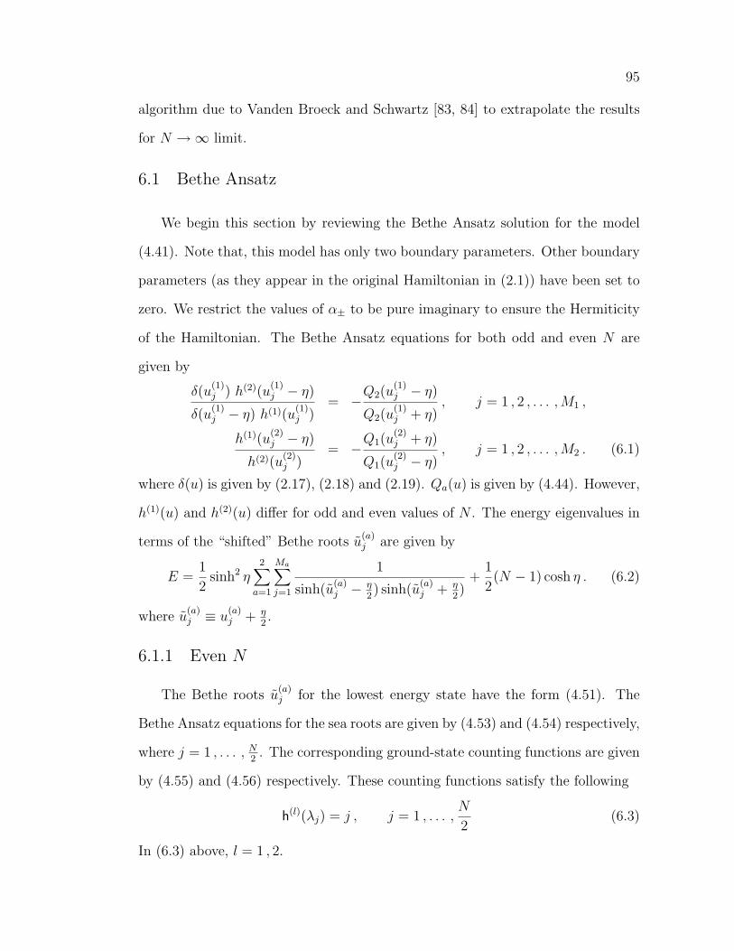
95
algorithm due to Vanden Broeck and Schwartz [83, 84] to extrapolate the results
for N →∞ limit.
6.1 Bethe Ansatz
We begin this section by reviewing the Bethe Ansatz solution for the model
(4.41). Note that, this model has only two boundary parameters. Other boundary
parameters (as they appear in the original Hamiltonian in (2.1)) have been set to
zero. We restrict the values of α± to be pure imaginary to ensure the Hermiticity
of the Hamiltonian. The Bethe Ansatz equations for both odd and even N are
given by
δ(u(1)j ) h(2)(u
(1)j − η)
δ(u(1)j − η) h(1)(u
(1)j )
= −Q2(u
(1)j − η)
Q2(u(1)j + η)
, j = 1 , 2 , . . . , M1 ,
h(1)(u(2)j − η)
h(2)(u(2)j )
= −Q1(u
(2)j + η)
Q1(u(2)j − η)
, j = 1 , 2 , . . . , M2 . (6.1)
where δ(u) is given by (2.17), (2.18) and (2.19). Qa(u) is given by (4.44). However,
h(1)(u) and h(2)(u) differ for odd and even values of N . The energy eigenvalues in
terms of the “shifted” Bethe roots u(a)j are given by
E =1
2sinh2 η
2∑a=1
Ma∑j=1
1
sinh(u(a)j − η
2) sinh(u
(a)j + η
2)
+1
2(N − 1) cosh η . (6.2)
where u(a)j ≡ u
(a)j + η
2.
6.1.1 Even N
The Bethe roots u(a)j for the lowest energy state have the form (4.51). The
Bethe Ansatz equations for the sea roots are given by (4.53) and (4.54) respectively,
where j = 1 , . . . , N2. The corresponding ground-state counting functions are given
by (4.55) and (4.56) respectively. These counting functions satisfy the following
h(l)(λj) = j , j = 1 , . . . ,N
2(6.3)
In (6.3) above, l = 1 , 2.

96
6.1.2 Odd N
In this section, we present an extension of the previous results to include
solutions for odd N values. The roots distribution is similar to the previous case,
but now we have M(1,1) = M(2,1) = N+12
, and M(1,2) = M(2,2) = p−12
. Using the
following in (6.1),
h(1)(u) = sinh(u− α+ + η) sinh(u + α+ + η)
× sinh2N+1(u + 2η) cosh2(u + η) cosh(u + 2η)
sinh(2u + 3η),
h(2)(u) = h(1)(−u− 2η) , (6.4)
we obtain the Bethe Ansatz equations
e1(λ(1,1)j )2N+1
[g1(λ
(1,1)j )e1+2a−(λ
(1,1)j )e1−2a−(λ
(1,1)j )
]−1(6.5)
= −(N+1)/2∏
k=1
[e2(λ
(1,1)j − λ
(2,1)k )e2(λ
(1,1)j + λ
(2,1)k )
]
×(p−1)/2∏
k=1
[g2(λ
(1,1)j − λ
(2,2)k )g2(λ
(1,1)j + λ
(2,2)k )
],
and
e1(λ(2,1)j )2N+1
[g1(λ
(2,1)j )e1+2a+(λ
(2,1)j )e1−2a+(λ
(2,1)j )
]−1(6.6)
= −(N+1)/2∏
k=1
[e2(λ
(2,1)j − λ
(1,1)k )e2(λ
(2,1)j + λ
(1,1)k )
]
×(p−1)/2∏
k=1
[g2(λ
(2,1)j − λ
(1,2)k )g2(λ
(2,1)j + λ
(1,2)k )
],
respectively, where j = 1 , . . . , N+12
. Note the presence of parameter-dependant
terms in both the equations above. One can also notice the number of extra roots
changes from p+12
to p−12
for Q1(u). The ground-state counting functions for this
case read
h(1)(λ) =1
2π
{(2N + 1)q1(λ)− r1(λ)− q1+2a−(λ)− q1−2a−(λ)

97
−(N+1)/2∑
k=1
[q2(λ− λ
(2,1)k ) + q2(λ + λ
(2,1)k )
]−
(p−1)/2∑k=1
[r2(λ− λ
(2,2)k ) + r2(λ + λ
(2,2)k )
] },
(6.7)
and
h(2)(λ) =1
2π
{(2N + 1)q1(λ)− r1(λ)− q1+2a+(λ)− q1−2a+(λ)
−(N+1)/2∑
k=1
[q2(λ− λ
(1,1)k ) + q2(λ + λ
(1,1)k )
]−
(p−1)/2∑k=1
[r2(λ− λ
(1,2)k ) + r2(λ + λ
(1,2)k )
] },
(6.8)
As for even N , we again have the following
h(l)(λj) = j , j = 1 , . . . ,N + 1
2(6.9)
where l = 1 , 2. Note that (6.3) and (6.9) can be written more compactly as
h(l)(λj) = j , j = 1 , . . . , bN + 1
2c (6.10)
where b. . .c denotes the integer part and µλbN+12
c is the largest sea root for that
“sea.” Subsequently, we shall denote largest sea roots as µΛl.
6.2 Finite-size correction of order 1/N
In this section, we shall compute the finite-size correction for the ground state
and low lying excited states. For these excited states, we restrict our analysis to
excitations by holes which are located to the right of the real sea roots. Applying
(4.51) to (6.2), we get the lowest state energy eigenvalues for chain of finite length
N ,
E = −π sin µ
µ
{1
2
2∑a=1
bN+12
c∑j=−bN+1
2c
a1(λ(a,1)j )− a1(0) +
2∑a=1
M(a,2)∑j=1
b1(λ(a,2)j )
}
+1
2(N − 1) cos µ . (6.11)
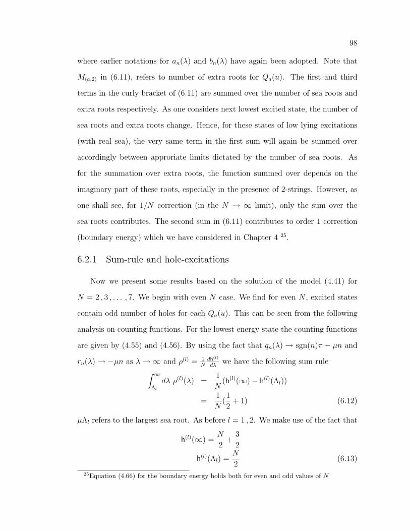
98
where earlier notations for an(λ) and bn(λ) have again been adopted. Note that
M(a,2) in (6.11), refers to number of extra roots for Qa(u). The first and third
terms in the curly bracket of (6.11) are summed over the number of sea roots and
extra roots respectively. As one considers next lowest excited state, the number of
sea roots and extra roots change. Hence, for these states of low lying excitations
(with real sea), the very same term in the first sum will again be summed over
accordingly between approriate limits dictated by the number of sea roots. As
for the summation over extra roots, the function summed over depends on the
imaginary part of these roots, especially in the presence of 2-strings. However, as
one shall see, for 1/N correction (in the N → ∞ limit), only the sum over the
sea roots contributes. The second sum in (6.11) contributes to order 1 correction
(boundary energy) which we have considered in Chapter 4 25.
6.2.1 Sum-rule and hole-excitations
Now we present some results based on the solution of the model (4.41) for
N = 2 , 3 , . . . , 7. We begin with even N case. We find for even N , excited states
contain odd number of holes for each Qa(u). This can be seen from the following
analysis on counting functions. For the lowest energy state the counting functions
are given by (4.55) and (4.56). By using the fact that qn(λ) → sgn(n)π − µn and
rn(λ) → −µn as λ →∞ and ρ(l) = 1N
dh(l)
dλwe have the following sum rule∫ ∞
Λl
dλ ρ(l)(λ) =1
N(h(l)(∞)− h(l)(Λl))
=1
N(1
2+ 1) (6.12)
µΛl refers to the largest sea root. As before l = 1 , 2. We make use of the fact that
h(l)(∞) =N
2+
3
2
h(l)(Λl) =N
2(6.13)
25Equation (4.66) for the boundary energy holds both for even and odd values of N

99
From (6.12) and (6.13), we see that there is one hole located to the right of the
largest sea root. Similar analysis for low lying (multi-hole) excited states yields
the following
∫ ∞
Λl
dλ ρ(l)(λ) =1
N(h(l)(∞)− h(l)(Λl))
=1
N(1
2+ NH) (6.14)
where NH is the number of holes (odd) to the right of the corresponding largest sea
root. To illustrate the results above, we consider the following low lying excited
states with N2−1 and N
2−2 sea roots and therefore different number of extra roots
than the lowest energy state 26. The former case is found to have one hole with
p−12
and p−32
extra roots in addition to a 2-string from each of the Q1(u) and Q2(u)
respectively. From,
h(l)(∞) =N
2+
1
2
h(l)(Λl) =N
2− 1 (6.15)
one has
1
N(h(l)(∞)− h(l)(Λl)) =
1
N(1
2+ 1) (6.16)
Hence giving NH = 1. The later case has three holes with p+12
and p−12
extra roots
and a 2-string from each of the Qa(u) with a = 1 , 2. Similar analysis,
h(l)(∞) =N
2+
3
2
h(l)(Λl) =N
2− 2 (6.17)
yields
1
N(h(l)(∞)− h(l)(Λl)) =
1
N(1
2+ 3) (6.18)
26The lowest energy state has N2 sea roots. As for the extra roots, there are p+1
2 and p−12 of
them for Q1(u) and Q2(u) respectively

100
giving NH = 3. The total number of roots are the same for all these states. There
are also excited states with equal number of sea and extra roots as for the state
of lowest energy, but with position of the single hole nearer to the origin than
that of the lowest energy state, suggesting the usual bulk hole-excitation scenario,
Ehole(λ(a)) increases as λ(a) → 0 where Ehole(λ
(a)) is the energy due to the presence
of holes and λ(a), with a = 1 , 2 denote the positions of the holes in both “seas.”
We shall compute the explicit expression for energy due to holes shortly.
As for the odd N case, we have the true ground state, namely state of lowest
energy without hole. From the counting functions, (6.7) and (6.8), we have∫ ∞
Λl
dλ ρ(l)(λ) =1
N(h(l)(∞)− h(l)(Λl))
=1
2N(6.19)
As before l = 1 , 2, and we make use of the fact that
h(l)(∞) =N
2+ 1
h(l)(Λl) =N + 1
2(6.20)
From (6.20), we see that this state of lowest energy for odd N has no hole, signifying
the true ground state. Similar analysis for low lying excited states yields the
following ∫ ∞
Λl
dλ ρ(l)(λ) =1
N(h(l)(∞)− h(l)(Λl))
=1
N(1
2+ NH) (6.21)
where NH is the number of holes (even) to the right of sea roots. Hence, for odd
N case, there are even number of holes (for each Qa(u)), with a = 1 , 2, for the
excited states, e.g., for the first excited state with N−12
sea roots,
h(l)(∞) =N + 1
2+
3
2
h(l)(Λl) =N − 1
2(6.22)

101
which signifies the presence of two holes.
It is known for simpler models of spin chains e.g., closed XXZ chain that even
number of holes are present in chains with even number of spins and vice versa.
Hence, the true ground state (lowest energy state with no holes) for these models
is found to lie in even N sector. The reverse scenario (one hole in the lowest energy
state for even N and ground state in odd N sector) we find here for this model can
be explained using some heuristic arguments based on spin and magnetic fields at
the two boundaries, similar to the one given at the end of Section 4.1 27. From
(4.67), we notice the signs of a+ and a− must be the same for boundary parameter
region of interest. Hence, in Hamiltonian (4.41), the direction of the magnetic fields
at the two boundaries are also the same (Both up or both down). This upsets the
antiferromagnetic spin arrangement at the boundaries, favouring spin allignments
along the same direction at the boundaries for chains with even N . This causes the
following: presence of odd N behaviours in the even N chain, namely the lowest
energy state for even N sector has one hole for each Qa(u). Spins at the boundaries
for the odd N chain will not experience such spin upset since the parallel magnetic
fields favours the antiferromagnetic arrangement of an odd N chain. Therefore,
the lowest energy state for odd N chain has no holes. In other words, the true
ground state exists in odd N sector. Further effects are the presence of odd and
even number of holes in chains with even and odd N respectively as shown in the
analysis above.
Now, the energy due to hole excitations can be presented. We consider first
the lowest energy state for even N case with one hole. Using
1
N
N2∑
k=−N2
g(λ− λ(a,1)k ) ≈
∫ ∞
−∞dλ′ ρ(l)(λ′)g(λ− λ′)− 1
Ng(λ− λ(a)) (6.23)
27Readers are urged to refer to Figures 4.2 and 4.3.

102
for some arbitrary function g(λ) and
ρ(l) =1
N
dh(l)
dλ(6.24)
where l = 1 , 2, µλ(a,1)k ≡ sea roots, with a = 1 , 2, and µλ(a) ≡ position of the hole
for each of the Qa(u), one can write down the sum of the two densities
ρ(1)(λ) + ρ(2)(λ) = 4a1(λ)−∫ ∞
−∞dλ′ (ρ(1)(λ′) + ρ(2)(λ′))a2(λ− λ′)
+1
N[a2(λ− λ(1)) + a2(λ− λ(2))] +
1
N[2a1(λ) + 2a2(λ)− 2b1(λ)
− a1+2a−(λ)− a1−2a−(λ)− a1+2a+(λ)− a1−2a+(λ)
−p−12∑
k=1
(b2(λ− λ(2,2)k ) + b2(λ + λ
(2,2)k ))
−p+12∑
k=1
(b2(λ− λ(1,2)k ) + b2(λ + λ
(1,2)k ))] (6.25)
Defining ρtotal(λ) ≡ ρ(1)(λ) + ρ(2)(λ) and solving (6.25) using Fourier transform,
we have
ρtotal(ω) = 4s(ω) +1
NR(ω)
+1
NJ(ω)(eiωλ(1)
+ eiωλ(2)
) (6.26)
where ρtotal(ω) , a2(ω) and s(ω) are the Fourier transforms of ρtotal(λ) , a2(λ) and
a1(λ)1+a2(λ)
respectively. Also J(ω) = a2(ω)1+a2(ω)
. R(ω) is the contribution from the second
square bracket in (6.25), which will not enter the calculation for Ehole(λ(a)) and
will be omitted henceforth. The Fourier transform of hole density are the third
and the fourth terms in (6.26), which gives
ρhole(λ) =1
N[J(λ− λ(1)) + J(λ− λ(2))] (6.27)
Using approximation (6.23) in (6.11), and making use of (6.27), one has
Ehole(λ(a)) = −Nπ sin µ
2µ
∫ ∞
−∞dλ a1(λ)ρhole(λ)
+π sin µ
2µ
2∑a=1
a1(λ(a)) (6.28)

103
which after some manipulation yields
Ehole(λ(a)) =
π sin µ
4µ
2∑a=1
1
cosh πλ(a)(6.29)
Generalizing the derivation to α number of holes, one has
ρhole(λ) =1
N
∑α
2∑a=1
J(λ− λ(a)α ) (6.30)
and finally the following for the energy
Ehole(λ(a)α ) =
π sin µ
4µ
∑α
2∑a=1
1
cosh πλ(a)α
(6.31)
Note that Ehole(λ(a)α ) increases as λ(a)
α → 0 as mentioned above in paragraph fol-
lowing (6.18).
6.2.2 Casimir energy
In this section, we give the derivation of 1/N correction (Casimir energy) to
the lowest energy state, for the even N case (with one hole). This result is then
generalized to include odd N values as well as the low lying (multi-hole) excited
states. We begin by presenting the expression for the density difference between
chain of finite length (with N spins), ρ(1)N (λ) + ρ
(2)N (λ) and that of infinite length,
ρ∞(λ)
ρ(1)N (λ) + ρ
(2)N (λ)− ρ∞(λ) = −
∫ ∞
−∞dγ a2(λ− γ)[
1
N
N2∑
β=−N2
δ(γ − λ(1,1)β )− ρ
(1)N (γ)]
−∫ ∞
−∞dγ a2(λ− γ)[
1
N
N2∑
β=−N2
δ(γ − λ(2,1)β )− ρ
(2)N (γ)]
−∫ ∞
−∞dγ a2(λ− γ)[ρ
(1)N (γ) + ρ
(2)N (γ)− ρ∞(γ)] (6.32)
In (6.32) and henceforth, only terms that are crucial to the computation of 1/N
correction are given. Other parameter dependant terms that contribute to order 1

104
correction have been omitted here 28. Solving (6.32) yields
ρ(1)N (λ) + ρ
(2)N (λ)− ρ∞(λ) = −
∫ ∞
−∞dγ p(λ− γ)[
1
N
N2∑
β=−N2
δ(γ − λ(1,1)β )− ρ
(1)N (γ)]
−∫ ∞
−∞dγ p(λ− γ)[
1
N
N2∑
β=−N2
δ(γ − λ(2,1)β )− ρ
(2)N (γ)]
(6.33)
where ρ∞(λ) = 4a1(λ)1+a2(λ)
≡ 4s(λ) and p(λ) = 12π
∫∞−∞ dω e−iωλ a2(ω)
1+a2(ω)Similar equation
expressing the energy difference between finite and infinite system is also needed
to compute Casimir energy. This is given by
EN − E∞ = −Nπ sin µ
2µ
{ ∫ ∞
−∞dλ a1(λ)[
1
N
N2∑
β=−N2
δ(λ− λ(1,1)β )− ρ
(1)N (λ)]
+∫ ∞
−∞dλ a1(λ)[
1
N
N2∑
β=−N2
δ(λ− λ(2,1)β )− ρ
(2)N (λ)]
+∫ ∞
−∞dλ a1(λ)[ρ
(1)N (λ) + ρ
(2)N (λ)− ρ∞(λ)]
}(6.34)
Using (6.33) and the fact that p(ω)a1(ω) = s(ω)a2(ω), we have
EN − E∞ = −Nπ sin µ
4µ
{ ∫ ∞
−∞dλ S
(1)N (λ)ρ(1)
∞ (λ) +∫ ∞
−∞dλ S
(2)N (λ)ρ(2)
∞ (λ)}
(6.35)
where S(l)N (λ) ≡ 1
N
∑N2
β=−N2
δ(λ−λ(l,1)β )− ρ
(l)N (λ) and ρ(l)
∞(λ) = 12ρ∞(λ) ≡ 2s(λ) with
l = 1 , 2. Further, using Euler-Maclaurin summation formula [86], (6.35) becomes
EN − E∞ = −Nπ sin µ
2µ
{−∫ ∞
Λ1
dλ ρ(1)∞ (λ)ρ
(1)N (λ) +
1
2Nρ(1)∞ (Λ1)
+1
12N2ρ(1)N (Λ1)
ρ(1)′
∞ (Λ1)−∫ ∞
Λ2
dλ ρ(2)∞ (λ)ρ
(2)N (λ) +
1
2Nρ(2)∞ (Λ2)
+1
12N2ρ(2)N (Λ2)
ρ(2)′
∞ (Λ2)}
(6.36)
28See [53] for details

105
(6.33) can also be expressed in similar form
ρ(1)N (λ) + ρ
(2)N (λ) − ρ∞(λ) =
∫ ∞
Λ1
dγ p(λ− γ)ρ(1)N (γ)− 1
2Np(λ− Λ1)
− p′(λ− Λ1)
12N2ρ(1)N (Λ1)
+∫ ∞
Λ2
dγ p(λ− γ)ρ(2)N (γ)− 1
2Np(λ− Λ2)
− p′(λ− Λ2)
12N2ρ(2)N (Λ2)
(6.37)
As before, µΛ1 and µΛ2 are the largest sea roots from the two “seas” respectively.
From this point, the calculation very closely resembles the details found in Section
2 in [57]. Hence, we omit the details and give only the crucial steps. Note that
(6.37) can be written in the standard form of the Wiener-Hopf equation [87] after
redefining the terms,
χ(1)(t) + χ(2)(t) −∫ ∞
0ds p(t− s)χ(1)(s)−
∫ ∞
0ds p(t− s)χ(2)(s)
≈ f (1)(t)− 1
2Np(t) +
1
12N2ρ(1)N (Λ1)
p′(t)
+ f (2)(t)− 1
2Np(t) +
1
12N2ρ(2)N (Λ2)
p′(t) (6.38)
where the following definitions have been adopted
χ(l)(λ) = ρ(l)N (λ + Λl)
f (l)(λ) = ρ(l)∞(λ + Λl) (6.39)
and following change in variable is used : t = λ − Λl with l = 1 , 2 From the
Fourier transformed version of (6.38), one can solve for X(l)+ (ω) which is the Fourier
transfrom of χ(l)+ (t) that is analytic in the upper half complex plane 29,
X(l)+ (ω) =
1
2N+
iω
12N2ρ(l)N (Λl)
+ G+(ω)( ig1
12N2ρ(l)N (Λl)
− 1
2N− iω
12N2ρ(l)N (Λl)
+2G+(iπ)e−πΛl
π − iω
)(6.40)
29Again for complete details, refer to [57]

106
where G+(ω)G+(−ω) = 1 + a2(ω) and g1 = i12
(2 + ν − 2νν−1
). For later use, note
that G+(0)2 = 2(ν−1)ν
.
From (6.12), (6.39) and (6.40), one can then determine ρ(1)N (Λl) and ρ
(2)N (Λ2) ex-
plicitly from
χ(l)+ (0) ≡ 1
2ρ
(l)N (Λl) =
1
2π
∫ ∞
−∞dω X
(l)+ (ω) (6.41)
by contour integration and some algebra. We give the result below
ρ(l)N (Λl) =
1
4N
{π + 2πα + ig1 + [π2 +
2ig1π
3− g2
1
3+ 4π2α2 + 4πα(π + ig1)]
12
}(6.42)
where α = 1G+(0)
= ( ν2(ν−1)
)12
Finally, using ρ(l)∞(λ) ≈ 2e−πλ for λ → Λl and (6.36), one arrives at the desired
expression for 1/N correction to the energy,
EN − E∞ = ECasimir = −π2 sin µ
24µN(1− 12α2) (6.43)
where the effective central charge is
ceff = 1− 12α2
= 1− 6ν
(ν − 1)(6.44)
We see that for this model, the central charge, c = 1 (Free boson). Also ceff is
independent of boundary parameters, unlike for the Dirichlet case [57]. This is
a feature expected for models with Neumann boundary condition. Further, from
conformal field theory, one also has the following for the conformal dimensions,
∆ =1− ceff
24
=ν
4(ν − 1)(6.45)
Note that the above results are derived for the lowest energy state for even N with
one hole for each Qa(u). Reviewing the derivation above, one can notice that the

107
results above can be further generalized for any N and for low lying excited states
with arbitrary number of holes, provided these holes are located to the right of the
largest sea root as mentioned in the beginning of Section 6.2. For these excited
states, the sum for S(l)N (λ) in (6.32) - (6.35) will inevitably have different limits
since the number of sea roots vary. However, after applying the Euler-Maclaurin
formula, one would recover (6.36) and (6.37). In addition to that, for states with
NH number of holes (all located to the right of the largest sea root), one uses the
more general result for the sum rule, namely (6.14) and (6.21) which eventually
yields
α =NH
G+(0)(6.46)
Thus, we have the following for the effective central charge and conformal dimen-
sions for low lying excited states
ceff = 1− 6ν
(ν − 1)N2
H
∆ =ν
4(ν − 1)N2
H (6.47)
Surprisingly, the results (6.45) and (6.47) appear to have more resemblance to spin
chains with diagonal boundary terms, as one could see from the νν−1
dependance
[78]-[81], rather than ν−1ν
[43] which is the anticipated form for conformal dimen-
sions for spin chains with nondiagonal boundary terms. Indeed the theory of a free
Bosonic field ϕ compactified on a circle of radius r is invariant under ϕ 7→ ϕ+2πr,
where r = 2β. β is the continuum bulk coupling constant that is related to ν by
β2 = 8π(ν−1ν
). Further, the quantization of the momentum zero-mode Π0, yields
Π0 = nβ2
for Neumann boundary condition and Π0 = 2nβ
for the Dirichlet case,
where n is an integer. Hence, the zero-mode contribution to the energy, E0,n ∼ Π20
implies E0,n ∼ ∆ ∼ (ν−1ν
) for Neumann and E0,n ∼ ∆ ∼ ( νν−1
) for Dirichlet case
respectively. More complete discussion on this topic can be found in [43, 80]. Next,

108
we will resort to numerical analysis to confirm our analytical results obtained in
this section.
6.3 Numerical results
We present here some numerical results for both odd and even N cases, to
support our analytical derivations in Section 6.2.2. We first solve numerically the
Bethe equations (6.1), (4.55), (4.56), (6.7) and (6.8) for some large number of spins.
We use these solutions to calculate Casimir energy numerically from the following
E = Ebulk + Eboundary + ECasimir (6.48)
In (6.48), E is given by (6.11). Thus, having determined the Bethe roots numer-
ically, one uses known expressions for Ebulk [13] and Eboundary [53] to determine
ECasimir. Then using the expression found above for ECasimir, namely (6.43), one
can determine the effective central charge, ceff for that value of N ,
ceff = − 24µN
π2 sin µ(E − Ebulk − Eboundary) (6.49)
Finally, we employ an algorithm due to Vanden Broeck and Schwartz [83, 84] to
extrapolate these values for central charge at N →∞ limit. Table 6.1 below shows
the ceff values for some finite even N , for the lowest energy state with one hole
(NH = 1). Equation (6.47) predicts ceff values of -11 and -7 for p = 1 and p = 3
30 respectively which are the extrapolated values (-11.000315 and -7.000410) we
obtain from the Vanden Broeck and Schwartz method.
For odd N sector, since NH = 0, (6.47) predicts ceff = 1 (for the ground
state) for any odd p. We present similar numerical results for odd N in Table 6.2
below for p = 1 and p = 3. We work out the ceff values numerically for N =
15 ,25 ,. . . ,65. Excellent agreement between the calculated and the extrapolated
values of 1.000770 and 1.001851 again strongly supports our analytical results.
30ν = p + 1

109
N ceff , p = 1 , ν = 2 ceff , p = 3 , ν = 416 -9.365620 -2.85387224 -9.857713 -3.27127932 -10.122128 -3.55714840 -10.287160 -3.77088248 -10.399970 -3.93955456 -10.481956 -4.07765264 -10.544233 -4.193784...
......
∞ -11.000315 -7.000410
Table 6.1: Central charge values, ceff for p = 1 (a+ = 0.783, a− = 0.859) and p = 3(a+ = 2.29, a− = 1.76), from numerical computations based on N = 16 ,24 ,. . . ,64and extrapolated values at N →∞ limit (Vanden Broeck and Schwartz algorithm).
N ceff , p = 1 , ν = 2 ceff , p = 3 , ν = 415 0.898334 0.53150125 0.936128 0.63401235 0.953433 0.69275845 0.963360 0.73184155 0.969797 0.76014265 0.974311 0.781795...
......
∞ 1.000770 1.001851
Table 6.2: Central charge values, ceff for p = 1 (a+ = 0.926, a− = 0.654) and p = 3(a+ = 2.10, a− = 1.80), from numerical computations based on N = 15 ,25 ,. . . ,65and extrapolated values at N →∞ limit (Vanden Broeck and Schwartz algorithm).
From the proposed Bethe equations for an open XXZ spin chain with nondi-
agonal boundary terms, we computed finite size effect, namely the 1/N correction
(Casimir energy) to the lowest energy state for both even and odd N . We also
studied the bulk excitations due to holes. We found some peculiar results for these
excitations of this model. Firstly, the number of holes for excited states seem to
be reversed: even number of holes for chains with odd number of spins and vice
versa. However, one could explain this by resorting to heuristic arguments involv-
ing effects of magnetic fields on the spins at the boundary. We then computed the
energy due to hole-excitations. We further generalized the finite-size correction

110
calculation to include multi-hole excited states, where these holes are situated to
the right of the largest sea root. Having found the correction, we proceeded to
compute the effective central charge, ceff and the conformal dimensions, ∆ for
the model. We found the central charge, c = 1. The effective central charge is
independent of the boundary parameters, as expected for models with Neumann
boundary condition. The result for ∆ however, turns out to be similar to mod-
els with diagonal boundary terms rather than the nondiagonal ones, to which the
model studied here belongs to.
As an independent check to our analytical results, we also solved the model
numerically for some large values of N . We used this solution to compute 1/N
correction for these large N values, then extrapolate them to the N → ∞ limit
using Vanden Broeck and Schwartz algorithm. Our numerical results strongly
support the analytical derivations presented here. Hence, the question about the
“Dirichlet-like” behaviour remains for now.
There are many other open questions that one can explore and address further.
For example, similar analysis involving boundary excitations can also be carried
out. This can be really challenging even for the diagonal (Dirichlet) case [79, 89].
Further, solution for more general XXZ model involving multiple Q(u) functions
[60, 61], can also be utilized in similar capacity to explore these effects. Last but
not least, excitations due to other objects that we choose to ignore here, such as
special roots/holes and so forth can also be explored for these models in order to
make the study more complete.

Chapter 7: Boundary S Matrix
Factorizable S matrix is an important object of integrable field theories and
integrable quantum spin chains. As for the “bulk” case where the S matrix is
determined in terms of two-particle scattering amplitudes, the “boundary” case
can equally well be formulated in terms of an analogous “one-particle boundary-
reflection” amplitude. These bulk and boundary amplitudes are required to satisfy
Yang-Baxter [1, 2, 3] and the boundary Yang-Baxter [5, 6] equations respectively.
Methods based on Bethe equations have long been used to compute bulk two-
particle S matrices [21, 90, 91]. In [21], Fadeev and Takhtajan studied scattering
of spinons for the periodic XXX chain for both the ferromagnetic and antiferro-
magnetic cases. The bulk two-particle S matrix for the latter case coincides with
the bulk S matrix for the sine-Gordon model [3] in the limit β2 → 8π, where β is
the sine-Gordon coupling constant. Much work has also been done on the subject
for open spin chains [42, 43, 78, 79], [92]–[95] as well as for integrable field theories
with boundary [6, 92]. In [6], Ghoshal and Zamolodchikov presented a precise
formulation of the concept of boundary S matrix for 1 + 1 dimensional quantum
field theory with boundaries such as Ising field theory with boundary magnetic
field and boundary sine-Gordon model. For the latter model, the authors used
a bootstrap approach to compute the boundary S matrix. They determined the
scalar factor up to a CDD-type of ambiguity. Nonlinear integral equation (NLIE)
[73, 74, 96] approach has also been used to study excitations in integrable quantum
field theories such as the sine-Gordon model [75]–[77],[97, 98] and open quantum
spin-1/2 XXZ spin chains [42, 43, 78, 79]. In fact, in [43], NLIE approach is used
111

112
to compute boundary S matrix for the open spin-1/2 XXZ spin chain with nondi-
agonal boundary terms, where the boundary parameters obey certain constraint.
The bulk anisoptopy parameter however is taken to be arbitrary.
In this chapter, we compute the eigenvalues of the boundary S matrix for
a special case of an open spin-1/2 XXZ spin chain with nondiagonal boundary
terms with two independant boundary parameters (with no constraint) at roots
of unity, using the solution obtained recently [51, 53]. The motivation for the
performed computation is the fact that the Bethe Ansatz equation for this model
is unchanged under sign reversal of the boundary parameters. Hence, the usual
trick of obtaining the second eigenvalue of the boundary S matrix of an open spin-
1/2 XXZ spin chain by exploiting the change in Bethe Ansatz equation under such
sign reversal of the boundary parameters [43, 93, 94, 95] would not work here.
Consequently, identifications of separate one-hole states are necessary here. We
follow the approach used earlier for diagonal open spin chains [93, 94]. This is
a generalization of the method developed by Korepin, Andrei and Destri [90, 91]
for computing bulk S matrix. The quantization condition discussed by Fendley
and Saleur [92] is a crucial step for the calculation. The solution utilized here was
derived for certain values of bulk anisotropy parameter, µ in the repulsive regime
(µ = πp+1
∈ (0, π2]) for odd p values. Hence, we focus only on the critical and
repulsive regime, which corresponds in the sine-Gordon model to β2 ∈ [4π, 8π) 31.
One-hole excitations for this model occur in even N sector [99] in contrast to the
diagonal open spin-1/2 XXZ spin chain where such excitations appear in the odd
N sector [94].
Since the Bethe roots for the model consist of “sea” roots and “extra” roots,
we rely on a conjectured relation between the “extra” roots and the hole rapidity,
31β2 = 8(π − µ)

113
which is confirmed numerically for system up to about 60 sites. We find that the
eigenvalue derived for the open XXZ spin chain agrees with one of the eigenval-
ues of Ghoshal-Zamolodchikov’s boundary S matrix for the one boundary sine-
Gordon model, provided the lattice boundary parameters that appear in the spin
chain Hamiltonian and the IR parameters that appear in Ghoshal-Zamolodchikov’s
boundary S matrix [6] obey the same relation as in [43] 32. The problem of finding
the second eigenvalue of the boundary S matrix requires the identification of an
independent one-hole state. In contrast to previous studies [43, 93, 94, 95], where
such state was found by reversing the signs of the boundary parameters 33, similar
strategy does not work here. Reversing the signs of the boundary parameters in the
present case leaves the Bethe equation unchanged, hence giving the same one-hole
state. Interestingly, a separate one-hole state with 2-string is found [99]. Using
a conjectured relation between “extra” roots, hole rapidity and the boundary pa-
rameters, which is again confirmed numerically for system up to about 60 sites, we
derive the remaining eigenvalue which also agrees with Ghoshal-Zamolodchikov’s
result.
7.1 One-hole state
In order to compute the spinon boundary scattering amplitude, we consider
a one-hole state. The roots distribution for such a state was found in [53]. One-
hole excitations for the open XXZ spin chain we study here appear in the even N
sector. Hence, it is sufficient to consider the results for even N case. The shifted
Bethe roots u(a)j = u
(a)j + η
2for this state have the form (4.51). The Bethe Ansatz
32Very recently, similar relations were found for the open XXZ spin chain with diagonal-nondiagonal boundary terms in [95].
33In fact, there is a change ξ± → −ξ± in the Bethe equation for the diagonal case [94].

114
equations are re-expressed in terms of counting functions, h(l)(λ) as
h(l)(λ(l,1)j ) = Jj, l = 1 , 2 (7.1)
where h(l)(λ) are given by (4.55) and (4.56). Further, {J1, J2, . . . , JN2} is a set of
increasing positive integers that parametrize the state 34. For states with no holes,
the integers take consecutive values. For one-hole state, there is a break in the
sequence, represented by a missing integer. This missing integer J , fixes the value
of the hole rapidity, λ, according to
h(1)(λ) = h(2)(λ) = J . (7.2)
If the hole is located to the right of the largest “sea” root (λ(a,1)N2
), then J =
bh(l)(∞)− h(l)(λ(a,1)N2
)c. See [99] for more details. For later use, we next define the
densities of sea roots as
ρ(l)(λ) =1
N
dh(l)(λ)
dλ(7.3)
where l = 1 , 2
7.2 One-hole state with 2-string
In addition to the one-hole state mentioned in last section, there is another
one-hole state. This state is the only remaining one-hole state, which also has a
2-string. In this section, we give some brief information on the state. The shifted
Bethe roots u(a)j = u
(a)j + η
2for this state have the following form
µλ(a,1)j j = 1 , 2 , . . . , M(a,1)
µλ(a,2)j + iπ
2, j = 1 , 2 , . . . , M(a,2)
µλ(a)0 + η
2
µλ(a)0 − η
2
, a = 1 , 2 , (7.4)
34In principle, there are two such sets of integers,{J
(1)i
}and
{J
(2)i
}corresponding to the two
counting functions, h(1)(λ) and h(2)(λ) respectively. But, in fact these two sets of integers areidentical. Hence we choose to drop the superscript, l from Jj in (7.1).

115
where λ(a)0 , µ = π
p+1and λ
(a,b)j are real. Here, M(1,1) = M(2,1) = N
2− 1, and
M(1,2) = p−12
, M(2,2) = p−32
. As before, µλ(a,1)j are the zeros of Qa(u) that form
real sea (“sea” roots) and µλ(a,2)k are real parts of the “extra” roots (also zeros of
Qa(u)) which are not part of the “seas.” For this state, we also have µλ(a)0 , the
real parts of additional “extra” roots that form a 2-string.
The counting functions for this state are given by
h(1)(λ) =1
2π
{(2N + 1)q1(λ)− r1(λ)− q1+2a−(λ)− q1−2a−(λ)− q1+2a+(λ)− q1−2a+(λ)
−N2−1∑
k=1
[q2(λ− λ
(2,1)k ) + q2(λ + λ
(2,1)k )
]−
(p−3)/2∑k=1
[r2(λ− λ
(2,2)k ) + r2(λ + λ
(2,2)k )
]−q3(λ− λ
(2)0 )− q3(λ + λ
(2)0 )− q1(λ− λ
(2)0 )− q1(λ + λ
(2)0 )
}, (7.5)
and
h(2)(λ) =1
2π
{(2N + 1)q1(λ)− r1(λ)
−N2−1∑
k=1
[q2(λ− λ
(1,1)k ) + q2(λ + λ
(1,1)k )
]−
(p−1)/2∑k=1
[r2(λ− λ
(1,2)k ) + r2(λ + λ
(1,2)k )
]−q3(λ− λ
(1)0 )− q3(λ + λ
(1)0 )− q1(λ− λ
(1)0 )− q1(λ + λ
(1)0 )
}. (7.6)
The Bethe Ansatz equations for this state take the following form,
h(l)(λ(l,1)j ) = Jj, l = 1 , 2 (7.7)
where {J1, J2, . . . , JN2−1} is a set of increasing positive integers that parametrize
the state. The hole for this state breaks the sequence, represented by a missing
integer. As before, the missing integer J ,enables one to calculate the hole rapidity,
λ using
h(1)(λ) = h(2)(λ) = J . (7.8)
If the hole appears to the right of the largest “sea” root (λ(a,1)N2−1
), then J = bh(l)(∞)−
h(l)(λ(a,1)N2−1
)c. More on this state can be found in [99].

116
7.3 Boundary S matrix
In this Section, we give the derivation for the boundary scattering amplitudes
for one-hole states reviewed in Section 6.1.
7.3.1 Eigenvalue for the one-hole state without 2-string
First, we consider the state reviewed in Section 7.1. From (4.55), (4.56), (7.3)
and (4.26), one can solve for the sum of the two densities. We recall the results
below [53],
ρtotal(λ) = ρ(1)(λ) + ρ(2)(λ)
= 4s(λ) +1
NR+(λ) (7.9)
where s(λ) = 12 cosh(πλ)
and R+(λ) is the inverse Fourier transform of R+(ω) which
is given by
R+(ω) =1
1 + a2(ω)
[2a1(ω) + 2a2(ω)− 2b1(ω)− a1+2a−(ω)− a1−2a−(ω)
− a1+2a+(ω)− a1−2a+(ω)− 2b2(ω)(
p−12∑
k=1
cos(λ(2,2)k ω) +
p+12∑
l=1
cos(λ(1,2)l ω))
+ 4a2(ω) cos(λω)]
(7.10)
The presence of extra roots, λ(a,2)k and the hole rapidity, λ, are to be noted here35.
Henceforth, we shall denote λ(a,2)k simply as λ
(a)k . Morever, momentum of the
excitation is given by
p(λ) = tan−1(sinh(πλ)
)− π
2(7.11)
From (7.11), one gets s(λ) = 12π
dp(λ)dλ
. Consequently, using (7.3), one rewrites (7.9)
as
1
N
dhtotal(λ)
dλ=
2
π
dp(λ)
dλ+
1
NR+(λ) (7.12)
35Energy carried by the hole is given by E(λ) = π sin µ2µ
1cosh(πλ)
. Such an expression for spinonwas derived in [21]

117
where htotal(λ) = h(1)(λ) + h(2)(λ) and 1N
dhtotal(λ)dλ
= ρtotal(λ). After integrating
(7.12) with respect to λ, taking limits of integration from 0 to λ, one finds 36
htotal(λ) = h(1)(λ) + h(2)(λ) =2
πNp(λ) +
∫ λ
0dλR+(λ) (7.13)
Since h(1)(λ) = h(2)(λ) ∈ positive integer and R+(λ) is an even function of λ,
multiplying the resulting expression by 2iπ and exponentiating gives
e2ip(λ)Neiπ2
∫ λ
−λdλR+(λ)
= 1 (7.14)
Next, let us compare equation (7.14) to the Yang’s quantization condition for a
particle on an interval of length N ,
e2ip(λ)NR(λ; a+)R(λ; a−) | λ, (±)〉 =| λ, (±)〉 (7.15)
where R(λ; a±) are the non-diagonal boundary S matrices and | λ, (±)〉 denote the
two possible one-hole states. Note that the ± in | λ, (±)〉 represents two posssible
one-hole states and not the right and left boundaries. The expression eiπ2
∫ λ
−λdλR+(λ)
then, should be equal to one of the two eigenvalues of the Yang matrix Y (λ) defined
by
Y (λ) = R(λ; a+)R(λ; a−) (7.16)
Defining this eigenvalue as α(λ, a+)α(λ, a−), where + and − denote the right and
left boundaries respectively, (7.14) can be rephrased as
e2ip(λ)Nα(λ, a+)α(λ, a−) = 1 (7.17)
The problem thus reduces to evaluating the following
α(λ, a+)α(λ, a−) = eiπ2
∫ λ
−λdλR+(λ)
(7.18)
36Since we are only able to determine the scattering amplitudes up to a rapidity-independentfactor, the additive constant p(0) from the integration is ignored in (7.13).

118
After some manipulations, we have the following,
α(λ, a+)α(λ, a−) = exp{2∫ ∞
0
dω
ωsinh(2iλω)
[ a2(ω)
1 + a2(ω)+
1
1 + a2(2ω)[a2(2ω)
+ a1(2ω)− b1(2ω)− 1
2(a1+2a−(2ω) + a1−2a−(2ω)
+ a1+2a+(2ω) + a1−2a+(2ω))
− b2(2ω)(
p−12∑
k=1
cos(2λ(2)k ω) +
p+12∑
l=1
cos(2λ(1)l ω))]
]}(7.19)
Further, using (4.30) and (4.31), one gets
α(λ, a+)α(λ, a−) = exp{2∫ ∞
0
dω
ωsinh(2iλω)
[2 sinh(3ω/2) sinh((ν − 2)ω/2)
sinh(2ω) sinh((ν − 1)ω/2)
+sinh(ω)
sinh((ν − 1)ω) cosh(ω)+
sinh((−ν + 2a− − 1)ω)
2 sinh((ν − 1)ω) cosh(ω)
+sinh((ν − 2a− − 1)ω)
2 sinh((ν − 1)ω) cosh(ω)+ (a− → a+)
+sinh(ω)
sinh((ν − 1)ω)(
p−12∑
k=1
cos(2λ(2)k ω) +
p+12∑
l=1
cos(2λ(1)l ω))
]}(7.20)
where (a− → a+) is a shorthand for two additional terms which are the same as
the third and fourth terms in the integrand of (7.20), but with a− replaced by a+.
The integrals involving “extra” roots λ(2)k and λ
(1)l yield
exp{2∫ ∞
0
dω
ωsinh(2iλω)
sinh(ω)
sinh((ν − 1)ω)(
p−12∑
k=1
cos(2λ(2)k ω) +
p+12∑
l=1
cos(2λ(1)l ω))
}
=
p−12∏
k=1
p+12∏
l=1
√f(λ
(2)k , λ
(1)l , λ)f(λ
(2)k , λ
(1)l , λ +
iπ
µ′)(7.21)
where µ′ = πν−1
and
f(λ(2)k , λ
(1)l , λ) =
sinh (µ′
2(λ + λ
(2)k + i
2− iπ
2µ′))
sinh (µ′
2(λ + λ
(2)k − i
2+ iπ
2µ′))
cosh (µ′
2(λ− λ
(2)k + i
2+ iπ
2µ′))
cosh (µ′
2(λ− λ
(2)k − i
2− iπ
2µ′))
×sinh (µ′
2(λ + λ
(1)l + i
2+ iπ
2µ′))
sinh (µ′
2(λ + λ
(1)l − i
2− iπ
2µ′))
cosh (µ′
2(λ− λ
(1)l + i
2− iπ
2µ′))
cosh (µ′
2(λ− λ
(1)l − i
2+ iπ
2µ′))
(7.22)

119
After evaluating the rest of the integrals, (7.20) becomes
α(λ, a+)α(λ, a−) = S0(λ)2S1(λ, a−)S1(λ, a+)
×p−12∏
k=1
p+12∏
l=1
√f(λ
(2)k , λ
(1)l , λ)f(λ
(2)k , λ
(1)l , λ +
iπ
µ′)
(7.23)
where
S0(λ) =1
πcosh(µ′λ)
∞∏n=0
Γ[
1ν−1
(4n + 1− 2iλ)]Γ[
1ν−1
(4n + 3− 2iλ) + 1]
Γ[
1ν−1
(4n + 1 + 2iλ)]Γ[
1ν−1
(4n + 3 + 2iλ) + 1]
×Γ[
1ν−1
(4n + 4 + 2iλ)]Γ[
1ν−1
(4n + 2iλ) + 1]
Γ[
1ν−1
(4n + 4− 2iλ)]Γ[
1ν−1
(4n− 2iλ) + 1]
×Γ2[
1ν−1
(2n− iλ) + 12
]Γ2[
1ν−1
(2n + 1 + iλ) + 12
]Γ2[
1ν−1
(2n + 2 + iλ) + 12
]Γ2[
1ν−1
(2n + 1− iλ) + 12
] (7.24)
S1(λ, a±) =1
π
√cosh(µ′(λ +
i
2(ν − 2a±))) cosh(µ′(λ− i
2(ν − 2a±)))
×∞∏
n=0
Γ[
1ν−1
(2n + 1 + iλ− 12(ν − 2a±)) + 1
2
]Γ[
1ν−1
(2n + 1− iλ− 12(ν − 2a±)) + 1
2
]×
Γ[
1ν−1
(2n + 1 + iλ + 12(ν − 2a±)) + 1
2
]Γ[
1ν−1
(2n + 1− iλ + 12(ν − 2a±)) + 1
2
]×
Γ[
1ν−1
(2n− iλ− 12(ν − 2a±)) + 1
2
]Γ[
1ν−1
(2n + 2 + iλ− 12(ν − 2a±)) + 1
2
]×
Γ[
1ν−1
(2n− iλ + 12(ν − 2a±)) + 1
2
]Γ[
1ν−1
(2n + 2 + iλ + 12(ν − 2a±)) + 1
2
] (7.25)
The values of the “extra” roots are dependant on the hole rapidity, λ and the
boundary parameters, a±. Hence, it is sensible to expect a relation between these
“extra” roots,{λ
(2)k , λ
(1)l
}, the boundary parameters, a± and the hole rapidity,
λ. Consequently, one needs to express the right hand side of (7.21) in terms of
purely a± and λ to complete the derivation. To look for this additional relation,

120
we begin with the information contained in the difference of the two densities,
ρ(1)(λ)− ρ(2)(λ). This leads to the following,
ρdiff (λ) = ρ(1)(λ)− ρ(2)(λ)
=1
NR−(λ) (7.26)
where R−(λ) has the following Fourier transform,
R−(ω) =1
1− a2(ω)
[− a1+2a−(ω)− a1−2a−(ω)− a1+2a+(ω)− a1−2a+(ω)
− 2b2(ω)(
p−12∑
k=1
cos(λ(2)k ω)−
p+12∑
l=1
cos(λ(1)l ω))
](7.27)
Analogous to (7.12)) one gets
1
N
dhdiff (λ)
dλ=
1
NR−(λ) (7.28)
where hdiff (λ) = h(1)(λ) − h(2)(λ) and 1N
dhdiff (λ)
dλ= ρdiff (λ). Further, integrating
(7.28) with respect to λ, taking limits of integration from 0 to λ as before, one
finds
hdiff (λ) = h(1)(λ)− h(2)(λ) =∫ λ
0dλR−(λ) (7.29)
Since h(1)(λ) = h(2)(λ) ∈ positive integer, using the fact that R−(λ) is an even
function of λ and exponentiating (7.29) we get
e∫ λ
−λdλR−(λ)
= g(λ, a+)g(λ, a−)
p−12∏
k=1
p+12∏
l=1
√√√√√ f(λ(2)k , λ
(1)l , λ)
f(λ(2)k , λ
(1)l , λ + iπ
µ′)
= 1 (7.30)
where g(λ, a±) ≡√
cosh( iµ′2
(ν−2a±))+i sinh(µ′λ)
cosh( iµ′2
(ν−2a±))−i sinh(µ′λ). Next, an important observation is the
following relation (as N →∞),
p−12∏
k=1
p+12∏
l=1
f(λ(2)k , λ
(1)l , λ) = −1 (7.31)

121
for which we provide numerical support in Table 7.1. Although the results shown
in Table 7.1 are computed for the case where the hole appears to the right of the
largest “sea” root, we find similar results for other hole locations. From (7.30) and
(7.31), it also follows that
p−12∏
k=1
p+12∏
l=1
f(λ(2)k , λ
(1)l , λ +
iπ
µ′) = −
(g(λ, a+)g(λ, a−)
)2
(7.32)
N∏ p−1
2k=1
∏ p+12
l=1 f(λ(2)k , λ
(1)l , λ), p = 3
∏ p−12
k=1
∏ p+12
l=1 f(λ(2)k , λ
(1)l , λ), p = 5
24 -0.999364 + 0.0356655 i -0.999334 + 0.036496 i32 -0.999421 + 0.0340133 i -0.999333 + 0.036522 i40 -0.999466 + 0.0326686 i -0.999334 + 0.036486 i48 -0.999502 + 0.0315413 i -0.999337 + 0.036419 i56 -0.999532 + 0.0305749 i -0.999340 + 0.036336 i64 -0.999558 + 0.0297318 i -0.999343 + 0.036243 i
Table 7.1:∏ p−1
2k=1
∏ p+12
l=1 f(λ(2)k , λ
(1)l , λ) for p = 3 (a+ = 2.1, a− = 1.6) and p = 5
(a+ = 3.3, a− = 2.7), from numerical solutions based on N = 24 ,32 ,. . . ,64.
We stress here that the values of λ(2)k and λ
(1)l used in computations above strictly
satisfy the Bethe equations (6.1). Finally, we can rewrite (7.23) as
α(λ, a+)α(λ, a−) = S0(λ)2S1(λ, a−)S1(λ, a+)g(λ, a+)g(λ, a−) (7.33)
up to a rapidity-independant phase factor. Subsequently, the complete expression
for each boundary’s scattering amplitude is given by (up to a rapidity-independant
phase factor)
α(λ, a±) = S0(λ)S1(λ, a±)g(λ, a±) (7.34)
where + and − again denotes right and left boundaries respectively.
7.3.2 Eigenvalue for the one-hole state with 2-string
We now consider the one-hole state with a 2-string, reviewed in Section 7.2.
The computation of the eigenvalue for this state is identical to the one given above.

122
Hence, we skip the details and present the result. Analogous to (7.20), we have
β(λ, a+)β(λ, a−) = exp{2∫ ∞
0
dω
ωsinh(2iλω)
[2 sinh(3ω/2) sinh((ν − 2)ω/2)
sinh(2ω) sinh((ν − 1)ω/2)
+sinh(ω)
sinh((ν − 1)ω) cosh(ω)+
sinh((−ν + 2a− − 1)ω)
2 sinh((ν − 1)ω) cosh(ω)
+sinh((ν − 2a− − 1)ω)
2 sinh((ν − 1)ω) cosh(ω)+ (a− → a+)
+sinh(ω)
sinh((ν − 1)ω)(
p−32∑
k=1
cos(2λ(2)k ω) +
p−12∑
l=1
cos(2λ(1)l ω))
+sinh(2ω)
sinh((ν − 1)ω)(cosh(2iλ
(1)0 ω) + cosh(2iλ
(2)0 ω))
]}(7.35)
which after evaluating the integrals yields
β(λ, a+)β(λ, a−) = S0(λ)2S1(λ, a−)S1(λ, a+)w(λ(1)0 , λ)w(λ
(2)0 , λ)
×p−32∏
k=1
p−12∏
l=1
√f(λ
(2)k , λ
(1)l , λ)f(λ
(2)k , λ
(1)l , λ +
iπ
µ′) (7.36)
where
w(λ(a)0 , λ) =
√√√√cosh(µ′(λ + λ(a)0 + i))
cosh(µ′(λ + λ(a)0 − i))
cosh(µ′(λ− λ(a)0 + i))
cosh(µ′(λ− λ(a)0 − i))
, a = 1 , 2 , (7.37)
As before, (a− → a+) represents two additional terms which are the same as the
third and fourth terms in the integrand of (7.35), but with a− replaced by a+. We
proceed to make the following conjecture to complete the derivation.
w(λ(1)0 , λ)w(λ
(2)0 , λ)
p−32∏
k=1
p−12∏
l=1
√f(λ
(2)k , λ
(1)l , λ)f(λ
(2)k , λ
(1)l , λ +
iπ
µ′) = g(λ +
iπ
µ′, a+)
× g(λ +iπ
µ′, a−)
(7.38)
Like (7.31), we provide numerical support for (7.38) in Table 7.2 where we compute
the ratio φ ≡ d1
d2, where d1 and d2 are the left hand side and the right hand side of
(7.38) respectively, for systems up to 64 sites. We believe this supports the validity

123
of (7.38) at N → ∞. The values of λ(2)k , λ
(1)l , λ
(1)0 and λ
(2)0 used in computations
are obtained by solving numerically the Bethe equations (7.5) and (7.6) for the
“sea” roots and (6.1) for the “extra” roots. The correctness and validity of such
numerical solutions are checked by comparing them with the ones obtained from
McCoy’s method for smaller number of sites, e.g., N = 2 , 4 and 6 37. We stress here
that although the results obtained in Table 7.2 are computed for J = 1, namely
the case where the hole appears close to the origin, similar results are found for
other hole locations, e.g., J = 2 , 3 , . . ..
N φ, p = 3 φ, p = 524 0.967073 + 0.254500 i 0.990295 + 0.138982 i32 0.981063 + 0.193688 i 0.994434 + 0.105361 i40 0.987716 + 0.156259 i 0.996308 + 0.085849 i48 0.991392 + 0.130928 i 0.997674 + 0.068166 i56 0.993634 + 0.112654 i 0.998065 + 0.062174 i64 0.995102 + 0.098852 i 0.998407 + 0.056428 i
Table 7.2: φ for p = 3 (a+ = 2.1, a− = 1.6) and p = 5 (a+ = 3.2, a− = 2.7), fromnumerical solutions based on N = 24 ,32 ,. . . ,64.
Using (7.38), the other eigenvalue for the Yang matrix (7.16) becomes
β(λ, a+)β(λ, a−) = S0(λ)2S1(λ, a+)S1(λ, a−)g(λ +iπ
µ′, a+)g(λ +
iπ
µ′, a−) (7.39)
hence giving the following for each boundary’s scattering amplitude (up to a
rapidity-independant phase factor),
β(λ, a±) = S0(λ)S1(λ, a±)g(λ +iπ
µ′, a±) (7.40)
7.3.3 Relation to boundary sine-Gordon model
Next, we briefly review Ghoshal-Zamolodchikov’s results for the one bound-
ary sine-Gordon theory [6]. We borrow conventions used in [43, 100]. Ghoshal-
37We are only able to use McCoy’s method to exactly solve for the Bethe roots for systems upto only 6 sites due to computer limitations.

124
Zamolodchikov’s results imply that the right and left boundary S matrices
R(θ ; η±, ϑ±, γ±) are given by
R(θ ; η, ϑ, γ) = r0(θ) r1(θ ; η, ϑ) M(θ ; η, ϑ, γ) , (7.41)
where M has matrix elements
M(θ ; η, ϑ, γ) =
(m11 m12
m21 m22
), (7.42)
where (η±, ϑ±, γ±) are the Ghoshal-Zamolodchikov’s IR parameters and θ is the
hole-rapidity. Further,
m11 = cos η cosh ϑ cosh(τθ) + i sin η sinh ϑ sinh(τθ) ,
m22 = cos η cosh ϑ cosh(τθ)− i sin η sinh ϑ sinh(τθ) ,
m12 = ieiγ sinh(τθ) cosh(τθ) ,
m21 = ie−iγ sinh(τθ) cosh(τθ) . (7.43)
where τ = 1ν−1
is the bulk coupling constant. The scalar factors have the following
integral representations [43, 100]
r0(θ) = exp
{2i∫ ∞
0
dω
ωsin(2θω/π)
sinh((ν − 2)ω/2) sinh(3ω/2)
sinh((ν − 1)ω/2) sinh(2ω)
},
r1(θ ; η, ϑ) =1
cos η cosh ϑσ(η, θ) σ(iϑ, θ) , (7.44)
where
σ(x, θ) = exp{
2∫ ∞
0
dω
ωsin((iπ − θ)ω/(2π)) sin(θω/(2π))
cosh((ν − 1)ωx/π)sinh((ν − 1)ω/2) cosh(ω/2)
}.
(7.45)
Our result (7.33) and (7.39) agree with the eigenvalues of
R(θ ; η+, ϑ+, γ+)R(θ ; η−, ϑ−, γ−), provided we make the following identification,
η± =µ′
2(ν − 2a±)
θ = πλ (7.46)
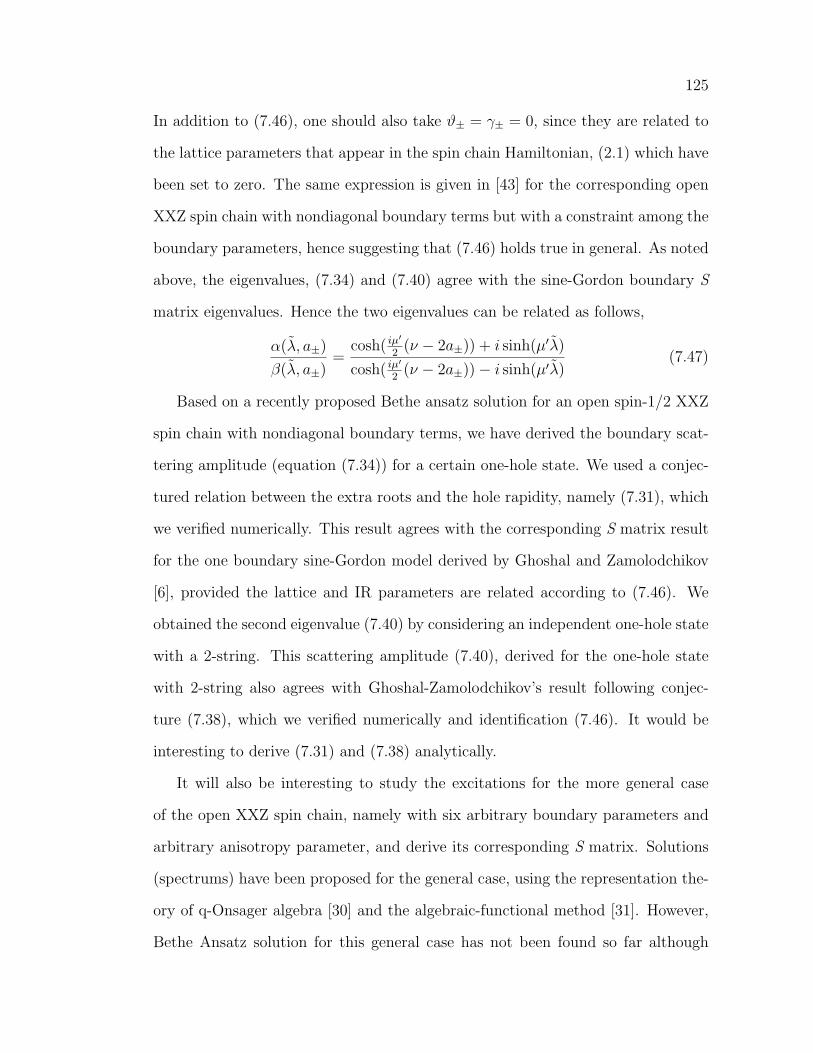
125
In addition to (7.46), one should also take ϑ± = γ± = 0, since they are related to
the lattice parameters that appear in the spin chain Hamiltonian, (2.1) which have
been set to zero. The same expression is given in [43] for the corresponding open
XXZ spin chain with nondiagonal boundary terms but with a constraint among the
boundary parameters, hence suggesting that (7.46) holds true in general. As noted
above, the eigenvalues, (7.34) and (7.40) agree with the sine-Gordon boundary S
matrix eigenvalues. Hence the two eigenvalues can be related as follows,
α(λ, a±)
β(λ, a±)=
cosh( iµ′
2(ν − 2a±)) + i sinh(µ′λ)
cosh( iµ′
2(ν − 2a±))− i sinh(µ′λ)
(7.47)
Based on a recently proposed Bethe ansatz solution for an open spin-1/2 XXZ
spin chain with nondiagonal boundary terms, we have derived the boundary scat-
tering amplitude (equation (7.34)) for a certain one-hole state. We used a conjec-
tured relation between the extra roots and the hole rapidity, namely (7.31), which
we verified numerically. This result agrees with the corresponding S matrix result
for the one boundary sine-Gordon model derived by Ghoshal and Zamolodchikov
[6], provided the lattice and IR parameters are related according to (7.46). We
obtained the second eigenvalue (7.40) by considering an independent one-hole state
with a 2-string. This scattering amplitude (7.40), derived for the one-hole state
with 2-string also agrees with Ghoshal-Zamolodchikov’s result following conjec-
ture (7.38), which we verified numerically and identification (7.46). It would be
interesting to derive (7.31) and (7.38) analytically.
It will also be interesting to study the excitations for the more general case
of the open XXZ spin chain, namely with six arbitrary boundary parameters and
arbitrary anisotropy parameter, and derive its corresponding S matrix. Solutions
(spectrums) have been proposed for the general case, using the representation the-
ory of q-Onsager algebra [30] and the algebraic-functional method [31]. However,
Bethe Ansatz solution for this general case has not been found so far although

126
such a solution has been proposed lately for the XXZ spin chain with six boundary
parameters at roots of unity [60]. In addition to the bulk excitations, one can
equally well look at boundary excitations although this can be rather challenging
even for the simpler case of spin chains with diagonal boundary terms [101].

Appendix 1
Here we briefly review the solution [27, 28] for the case that the constraint (2.3)
is satisfied, in order to facilitate comparison with the new cases considered in text.
The matrix M is then given by
M =
Λ(u) −h(−u− η) 0 . . . 0 −h(u)
−h(u + η) Λ(u + η) −h(−u− 2η) . . . 0 0...
......
. . ....
...−h(−u− (p + 1)η) 0 0 . . . −h(u + pη) Λ(u + pη)
(A1.1)
where h(u) must satisfy
h(u + iπ) = h (u + (p + 1)η) = h(u) , (A1.2)
h(u + η) h(−u− η) = δ(u) , (A1.3)p∏
j=0
h(u + jη) +p∏
j=0
h(−u− jη) = f(u) . (A1.4)
A pair of solutions is given by h(u) = h(±)(u) = h0(u)h(±)1 (u) with h0(u) given by
(3.23), and h(±)1 (u) given by
h(±)1 (u) = (−1)N+14 sinh(u± α−) cosh(u± β−) sinh(u± α+) cosh(u± β+)(A1.5)
Indeed, h0(u) satisfies
h0(u + η) h0(−u− η) = δ0(u) ,p∏
j=0
h0(u + jη) =p∏
j=0
h0(−u− jη) = f0(u) , (A1.6)
where δ0(u) is given by (2.18), and f0(u) is given by (2.21) and (2.23) for p even
and odd, respectively. Moreover, h(±)1 (u) satisfies
h(±)1 (u + η) h
(±)1 (−u− η) = δ1(u) , (A1.7)
127

128
where δ1(u) is given by (2.19); and
p∏j=0
h(±)1 (u + jη) +
p∏j=0
h(±)1 (−u− jη) = f1(u)− (−1)p(N+1)21−2p sinh2 (2(p + 1)u))
×[(−1)N cosh ((p + 1)(α− + α+ + β− + β+)) + cosh ((p + 1)(θ− − θ+))
],
(A1.8)
where f1(u) is given by (2.22) and (2.24) for p even and odd, respectively. Hence,
if the constraint (2.3) is satisfied, then the RHS of (A1.8) reduces to f1(u); hence,
all the conditions (A1.2)-(A1.4) are fulfilled. The corresponding expression for the
transfer matrix eigenvalues is given by
Λ(±)(u) = h(±)(u)Q(±)(u− η)
Q(±)(u)+ h(±)(−u− η)
Q(±)(u + η)
Q(±)(u), (A1.9)
with
Q(±)(u) =M(±)∏j=1
sinh(u− u(±)j ) sinh(u + u
(±)j + η) ,
M (±) =1
2(N − 1± k) , (A1.10)
and Bethe Ansatz equations
h(±)(u(±)j )
h(±)(−u(±)j − η)
= −Q(±)(u
(±)j + η)
Q(±)(u(±)j − η)
, j = 1 , . . . , M (±) . (A1.11)

Appendix 2
The coefficients µk appearing in the function Y (u) (5.13) are given as follows.
For p even,
µ0 = 2−4p
{− 1− cosh2((p + 1)(θ− − θ+))
− cosh(2(p + 1)α−) cosh(2(p + 1)α+) + cosh(2(p + 1)α−) cosh(2(p + 1)β−)+ cosh(2(p + 1)α+) cosh(2(p + 1)β−) + cosh(2(p + 1)α−) cosh(2(p + 1)β+)+ cosh(2(p + 1)α+) cosh(2(p + 1)β+)− cosh(2(p + 1)β−) cosh(2(p + 1)β+)
+[cosh((p + 1)(α− + α+)) cosh((p + 1)(β− − β+))
− cosh((p + 1)(α− − α+)) cosh((p + 1)(β− + β+))]2
+ 2(−1)N cosh((p + 1)(θ− − θ+))[cosh((p + 1)(α− − α+)) cosh((p + 1)(β− − β+))
− cosh((p + 1)(α− + α+)) cosh((p + 1)(β− + β+))]}
,
µ1 = 21−4p
{cosh((p + 1)(α− − α+))
[cosh((p + 1)(α− + α+))
+ (−1)N cosh((p + 1)(β− + β+)) cosh((p + 1)(θ− − θ+))]
− cosh((p + 1)(β− − β+))[cosh((p + 1)(β− + β+))
+ (−1)N cosh((p + 1)(α− + α+)) cosh((p + 1)(θ− − θ+))]}
,
µ2 = 2−4p sinh2((p + 1)(θ− − θ+)) . (A2.1)
For p odd,
µ0 = 2−4p
{− 1− cosh2((p + 1)(θ− − θ+))
− cosh(2(p + 1)α−) cosh(2(p + 1)α+)− cosh(2(p + 1)α−) cosh(2(p + 1)β−)− cosh(2(p + 1)α+) cosh(2(p + 1)β−)− cosh(2(p + 1)α−) cosh(2(p + 1)β+)
129

130
− cosh(2(p + 1)α+) cosh(2(p + 1)β+)− cosh(2(p + 1)β−) cosh(2(p + 1)β+)
+[cosh((p + 1)(α− + α+)) cosh((p + 1)(β− − β+))
+ cosh((p + 1)(α− − α+)) cosh((p + 1)(β− + β+))]2
− 2(−1)N cosh((p + 1)(θ− − θ+))[cosh((p + 1)(α− − α+)) cosh((p + 1)(β− − β+))
+ cosh((p + 1)(α− + α+)) cosh((p + 1)(β− + β+))]}
,
µ1 = 21−4p
{cosh((p + 1)(α− + α+))
[cosh((p + 1)(α− − α+))
+ (−1)N cosh((p + 1)(β− − β+)) cosh((p + 1)(θ− − θ+))]
+ cosh((p + 1)(β− + β+))[cosh((p + 1)(β− − β+))
+ (−1)N cosh((p + 1)(α− − α+)) cosh((p + 1)(θ− − θ+))]}
,
µ2 = 2−4p sinh2((p + 1)(θ− − θ+)) . (A2.2)
The modified function f(u) for the case η = iπp/(p + 1), with p a positive
integer
f0(u) = (−1)N2−2pN sinh2N ((p + 1)u) ,
f1(u) = (−1)N23−2p(
− sinh ((p + 1)α−) cosh ((p + 1)β−) sinh ((p + 1)α+) cosh ((p + 1)β+) cosh2 ((p + 1)u)+ cosh ((p + 1)α−) sinh ((p + 1)β−) cosh ((p + 1)α+) sinh ((p + 1)β+) sinh2 ((p + 1)u)
− cosh ((p + 1)(θ− − θ+)) sinh2 ((p + 1)u) cosh2 ((p + 1)u))
. (A2.3)
Correspondingly, the coefficients µ0 and µ1 are given by (A2.1) with the factor
(−1)N replaced by −1. Apart from these changes, the solution is the same as for
the case (2.70) for both odd and even p.
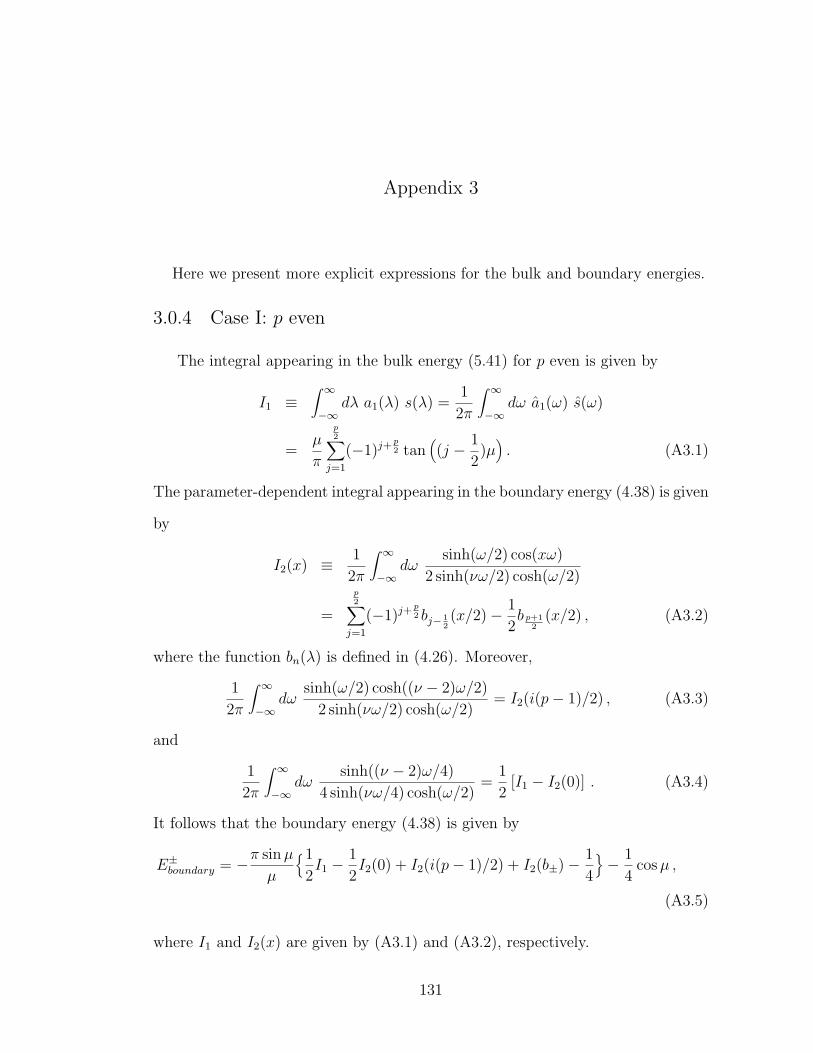
Appendix 3
Here we present more explicit expressions for the bulk and boundary energies.
3.0.4 Case I: p even
The integral appearing in the bulk energy (5.41) for p even is given by
I1 ≡∫ ∞
−∞dλ a1(λ) s(λ) =
1
2π
∫ ∞
−∞dω a1(ω) s(ω)
=µ
π
p2∑
j=1
(−1)j+ p2 tan
((j − 1
2)µ). (A3.1)
The parameter-dependent integral appearing in the boundary energy (4.38) is given
by
I2(x) ≡ 1
2π
∫ ∞
−∞dω
sinh(ω/2) cos(xω)
2 sinh(νω/2) cosh(ω/2)
=
p2∑
j=1
(−1)j+ p2 bj− 1
2(x/2)− 1
2b p+1
2(x/2) , (A3.2)
where the function bn(λ) is defined in (4.26). Moreover,
1
2π
∫ ∞
−∞dω
sinh(ω/2) cosh((ν − 2)ω/2)
2 sinh(νω/2) cosh(ω/2)= I2(i(p− 1)/2) , (A3.3)
and
1
2π
∫ ∞
−∞dω
sinh((ν − 2)ω/4)
4 sinh(νω/4) cosh(ω/2)=
1
2[I1 − I2(0)] . (A3.4)
It follows that the boundary energy (4.38) is given by
E±boundary = −π sin µ
µ
{1
2I1 −
1
2I2(0) + I2(i(p− 1)/2) + I2(b±)− 1
4
}− 1
4cos µ ,
(A3.5)
where I1 and I2(x) are given by (A3.1) and (A3.2), respectively.
131

132
3.0.5 Case II: p odd
The integral appearing in the bulk energy (5.41) for p odd is given by
I1 ≡∫ ∞
−∞dλ a1(λ) s(λ) =
1
2π
∫ ∞
−∞dω a1(ω) s(ω)
=µ
π2
[1 + 2µ
p−12∑
j=1
j cot(jµ)]. (A3.6)
The parameter-dependent integral appearing in the boundary energy (4.66) is given
by
I2(x) ≡ 1
2π
∫ ∞
−∞dω
sinh(ω/2) cosh(xω)
2 sinh(νω/2) cosh(ω/2)
=(−1)
p−12 µ
π sin(xπ)
x +
p−12∑
j=1
(−1)j cot(jµ) sin(2xjµ)
. (A3.7)
Moreover,
1
2π
∫ ∞
−∞dω
cosh((ν − 2)ω/4)
4 cosh(νω/4) cosh(ω/2)=
1
2[I1 + I2(0)] . (A3.8)
It follows that the boundary energy (4.66) is given by
E±boundary = −π sin µ
µ
{1
2I1 +
1
2I2(0) + I2((p + 1− 2|a±|)/2)− 1
4
}− 1
4cos µ ,(A3.9)
where I1 and I2(x) are given by (A3.6) and (A3.7), respectively.

Bibliography
[1] C. N. Yang, Phys. Rev. Lett. 19, 1312 (1967).
[2] R. J. Baxter, Ann. Phys. 70, 193 (1972); J. Stat. Phys. 8, 25 (1973); Exactly
Solved Models in Statistical Mechanics (Academic Press, 1982).
[3] A. B. Zamolochikov and Al. B. Zamolodchikov, Ann. Phys. 120, 253 (1979).
[4] A. B. Zamolodchikov, unpublished.
[5] I. V. Cherednik, Theor. Math. Phys. 61, 977 (1984).
[6] S. Ghoshal and A.B. Zamolodchikov, Int. J. Mod. Phys. A9, 3841 (1994)
[hep-th/9306002].
[7] W. Heisenberg, Z. Phys. 49, 619 (1928).
[8] H. Bethe, Z. Phys. 71, 205 (1931).
[9] L. Hulthen, Arkiv Mat., Astron. Fysik 26A, 1 (1938).
[10] J. Des Cloizeaux and J. J. Pearson, Phys. Rev. 128, 2131 (1962).
[11] R. Orbach, Phys. Rev. 112, 309 (1958).
[12] C. N. Yang and C. P. Yang, Phys. Rev. 150, 321 (1966).
[13] C. N. Yang and C. P. Yang, Phys. Rev. 150, 327 (1966).
[14] M. Gaudin, Phys. Rev. A4, 386 (1971); La fonction d’onde de Bethe (Masson,
1983).
133

134
[15] F.C. Alcaraz, M.N. Barber, M.T. Batchelor, R.J. Baxter and G.R.W. Quispel,
J. Phys. A20, 6397 (1987).
[16] E. Lieb and W. Liniger, Phys. Rev. 130, 1605 (1963).
[17] P. P. Kulish and E. K. Sklyanin, Phys. Lett. 70A, 461 (1979).
[18] E. K. Sklyanin, L. A. Takhtadzhyan and L. D. Faddeev, Teor. Mat. Fiz. 40,
194 (1979).
[19] L.D. Faddeev and L.A. Takhtajan, Russ. Math Surv. 34, 11 (1979).
[20] L. D. Faddeev, Soviet Scientific Reviews, Harvard Academic, London, 107
(1980).
[21] L. D. Fadeev and L. A. Takhtajan, J. Sov. Math. 24, 241 (1984).
[22] V. E. Korepin, N. M. Bogoliubov and A. G. Izergin, Quantum Inverse Scat-
tering Method, Correlation Functions and Algebraic Bethe Ansatz (Cambridge
University Press, 1993).
[23] E.K. Sklyanin, J. Phys. A21, 2375 (1988).
[24] J. Cao, H.-Q. Lin, K.-J. Shi and Y. Wang, Nucl. Phys. B663, 487 (2003)
[cond-mat/0212163].
[25] R.I. Nepomechie, J. Phys. A34, 9993 (2001) [hep-th/0110081].
[26] R.I. Nepomechie, Nucl. Phys. B622, 615 (2002); Addendum, Nucl. Phys.
B631, 519 (2002) [hep-th/0110116].
[27] R.I. Nepomechie, J. Stat. Phys. 111, 1363 (2003) [hep-th/0211001];
R.I. Nepomechie, J. Phys. A37, 433 (2004) [hep-th/0304092].

135
[28] R.I. Nepomechie and F. Ravanini, J. Phys. A36, 11391 (2003); Addendum,
J. Phys. A37, 1945 (2004) [hep-th/0307095].
[29] W.-L. Yang, R.I. Nepomechie and Y.-Z. Zhang, Phys. Lett. B633, 664 (2006)
[hep-th/0511134].
[30] P. Baseilhac, K. Koizumi, JSTAT P09006 (2007) [hep-th/0703106].
[31] W. Galleas, Nucl. Phys. B790, 524 (2008) [0708.0009].
[32] H.J. de Vega and A. Gonzalez-Ruiz, J. Phys. A26, L519 (1993)
[hep-th/9211114].
[33] G. Albertini, S. Dasmahapatra and B. McCoy, Int. J. Mod. Phys. A 7, Suppl.
1A (1992) 1; also published in “Infinite Analysis, ‘’ Adv. Ser. Math. Phys. 16,
eds A. Tsuchiya, T. Eguchi and M.Jimbo, (World Scientific, Singapore 1992).
[34] K. Fabricius and B.M. McCoy, J. Stat. Phys. 103 (2001) 647.
[35] R.J. Baxter, Ann. Phys. 76, 1-24, 25-47, 48-71 (1973).
[36] P.P. Kulish and E.K. Sklyanin, Lecture Notes in Physics, Vol. 151, 61
(Springer, 1982); P.P. Kulish, N.Yu. Reshetikhin and E.K. Sklyanin, Lett.
Math. Phys. 5, 393 (1981); P.P. Kulish and N.Yu. Reshetikhin, J. Sov. Math.
23, 2435 (1983); A.N. Kirillov and N.Yu. Reshetikhin, J. Sov. Math. 35, 2627
(1986); J. Phys. A20, 1565 (1987); L. Mezincescu and R.I. Nepomechie, J.
Phys. A25, 2533 (1992); Y.-K. Zhou, Nucl. Phys. B458, 504 (1996).
[37] R.J. Baxter and P.A. Pearce, J. Phys. A15, 897 (1982).
[38] V.V. Bazhanov and N.Yu. Reshetikhin, Int. J. Mod. Phys. A4, 115 (1989).
[39] R.J. Baxter, Adv. Stud. Pure Math. 19, 95 (1989).

136
[40] V.V. Bazhanov, S.L. Lukyanov and A.B. Zamolodchikov, Commun. Math.
Phys. 177, 381 (1996) [hep-th/9412229]; Commun. Math. Phys. 200, 297
(1999) [hep-th/9805008].
[41] A. Kuniba, K. Sakai and J. Suzuki, Nucl. Phys. B525, 597 (1998)
[math/9803056].
[42] C. Ahn and R.I. Nepomechie, Nucl. Phys. B676, 637 (2004)
[hep-th/0309261].
[43] C. Ahn, Z. Bajnok, R.I. Nepomechie, L. Palla and G. Takacs, Nucl. Phys.
B714, 307 (2005) [hep-th/0501047].
[44] A. Doikou, Nucl. Phys. B668, 447 (2003) [hep-th/0303205]; J. de Gier and
P. Pyatov, JSTAT P04002 (2004) [hep-th/0312235]; W. Galleas and M.J.
Martins, Phys. Lett. A335, 167 (2005) [nlin/0407027]; C.S. Melo, G.A.P.
Ribeiro and M.J. Martins, Nucl. Phys. B711, 565 (2005) [hep-th/0411038];
W.-L. Yang and Y.-Z. Zhang, JHEP 01, 021 (2005) [hep-th/0411190].
[45] A. Doikou and P.P. Martin, JSTAT P06004 (2006) [hep-th/0503019];
A. Doikou, JSTAT P09010 (2006) [hep-th/0603112].
[46] A. Nichols, V. Rittenberg and J. de Gier, JSTAT P05003 (2005)
[cond-mat/0411512];
J. de Gier, A. Nichols, P. Pyatov and V. Rittenberg, Nucl. Phys. B729, 387
(2005) [hep-th/0505062];
J. de Gier and F.H.L. Essler, Phys. Rev. Lett. 95, 240601 (2005)
[cond-mat/0508707].
[47] W.-L. Yang, Y.-Z. Zhang and M. Gould, Nucl. Phys. B698, 503 (2004)
[hep-th/0411048];

137
W.-L. Yang, Y.-Z. Zhang and R. Sasaki, Nucl. Phys. B729, 594 (2005)
[hep-th/0507148];
W.-L. Yang and Y.-Z. Zhang, Nucl. Phys. B744, 312 (2006)
[hep-th/0512154].
[48] P. Baseilhac and K. Koizumi, JSTAT P10005 (2005) [hep-th/0507053];
P. Baseilhac, [math-ph/0604036].
[49] A. Nichols, JSTAT P01003 (2006) [hep-th/0509069];
A. Nichols, JSTAT L02004 (2006) [hep-th/0512273 ].
[50] Z. Bajnok, JSTAT P06010 (2006) [hep-th/0601107].
[51] R. Murgan and R.I. Nepomechie, JSTAT P05007 (2005); Addendum, JSTAT
P11004 (2005) [hep-th/0504124].
[52] R. Murgan and R.I. Nepomechie, JSTAT P08002 (2005) [hep-th/0507139].
[53] R. Murgan, R.I. Nepomechie and C. Shi, Ann. Henri Poincare 7, 1429 (2006)
[hep-th/0512058].
[54] U. Bilstein and B. Wehefritz, J. Phys. A32, 191 (1999) [cond-mat/9807166];
U. Bilstein, J. Phys. A33, 4437 (2000) [cond-mat/0002162]; U. Bilstein, J.
Phys. A33, 7661 (2000) [cond-mat/0004484].
[55] U. Bilstein and V. Rittenberg, J. Phys. A33, L381 (2000)
[cond-mat/0004241].
[56] M. Takahashi and M. Suzuki, Prog. Theor. Phys. 48, 2187 (1972).
[57] C.J. Hamer, G.R.W. Quispel and M.T. Batchelor, J. Phys. A20, 5677 (1987).

138
[58] H.M. Babujian, Nucl. Phys. B215, 317 (1983); L.A. Takhtajan, Phys. Lett.
87A, 479 (1982).
[59] Al.B. Zamolodchikov, invited talk at the 4th Bologna Workshop, June 1999;
Z. Bajnok, L. Palla and G. Takacs, Nucl. Phys. B622, 565 (2002)
[hep-th/0108157].
[60] R. Murgan, R.I. Nepomechie and C. Shi, JSTAT P08006 (2006)
[hep-th/0605223].
[61] R. Murgan, R.I. Nepomechie and C. Shi JHEP 0701, 038 (2007)
[hep-th/0611078].
[62] I. Affleck, Phys. Rev. Lett. 56, 746 (1986).
[63] H.W.J. Blotte, J.L. Cardy and M.P. Nightingale, Phys. Rev. Lett. 56, 742
(1986).
[64] G. von Gehlen, V. Rittenberg and H. Ruegg, J. Phys. A19, 107 (1986).
[65] J.L. Cardy, J. Phys. A17, L385 (1984); Nucl. Phys. B 270, 186 (1986); J.
Phys. A19, L1093 (1986).
[66] H.J. de Vega and F. Woynarovich, Nucl. Phys. B251, 439 (1985).
[67] C.J. Hamer, J. Phys. A19, 3335 (1986).
[68] H.J. de Vega, J. Phys. A20, 6023 (1987).
[69] F. Woynarovich and H-P Eckle, J. Phys. A20, L97 (1987).
[70] F. Woynarovich Phys. Rev. Lett. 59, 259 (1987); Erratum, Phys. Rev. Lett.
59, 1264 (1987).

139
[71] V.I. Inozemtsev and B-D Dorfel, J. Phys. A26, L999 (1993).
[72] B-D Dorfel and St Meissner, J. Phys. A30, 1831 (1997) [hep-th/9609134].
[73] A. Klumper and M.T. Batchelor, J. Phys. A23, L189 (1990);
A. Klumper and P.A. Pearce, J. Stat. Phys. 64, 13 (1991);
A. Klumper, M.T. Batchelor and P.A. Pearce, J. Phys. A24, 3111 (1991).
[74] C. Destri and H.J. de Vega, Phys. Rev. Lett. 69, 2313 (1992).
[75] C. Destri and H. J. De Vega, Nucl. Phys. B504, 621 (1997) [hep-th/9701107].
[76] G. Feverati, F. Ravanini and G. Takacs, Nucl. Phys. B540, 543 (1999)
[hep-th/9805117].
[77] G. Feverati, [hep-th/0001172].
[78] A. LeClair, G.Mussardo, H. Saleur and S. Skorik, Nucl. Phys. B453, 581
(1995) [hep-th/9503227].
[79] C. Ahn, M. Bellacosa and F. Ravanini, Phys. Lett. B595, 537 (2004)
[hep-th/0312176].
[80] H. Saleur, [cond-mat/9812110].
[81] I. Affleck, M. Oshikawa and H. Saleur, Nucl. Phys. B594, 535 (2001)
[cond-mat/0009084].
[82] C. Ahn, R.I. Nepomechie and J. Suzuki, Nucl. Phys. B767, 250 (2007)
[hep-th/0611136].
[83] J-M van den Broeck and L.W Schwartz, SIAM J. Math. Anal. 10, 658 (1979).
[84] C.J. Hamer and M.N. Barber, J. Phys. A14, 2009 (1981).

140
[85] M. Henkel and G. Schutz, J. Phys. A21, 2617 (1988).
[86] E.T. Whittaker and G.N. Watson, A Course of Modern Analysis (Cambridge
University Press, 1988).
[87] P.M. Morse and H. Feshbach, Methods of Theoretical Physics (New York:
McGraw-Hill, 1953).
[88] R.I. Nepomechie, private communication.
[89] S. Skorik and H. Saleur, J. Phys. A28, 6605 (1995) [hep-th/9502011].
[90] V. E. Korepin, Theor. Math. Phys. 41, 953 (1979).
[91] N. Andrei and C. Destri, Nucl. Phys. B231, 445 (1984).
[92] P. Fendley and H. Saleur, Nucl. Phys. B428, 681 (1994) [hep-th/9402045].
[93] M. T. Grisaru, L. Mezincescu and R. I. Nepomechie, J. Phys. A28, 1027
(1995) [hep-th/9407089].
[94] A. Doikou and R. I. Nepomechie, J. Phys. A32, 3663 (1999)
[hep-th/9903066].
[95] A. Doikou, [0711.0716].
[96] C. Destri and H. J. De Vega, Nucl. Phys. B438, 413 (1995) [hep-th/9407117].
[97] D. Fioravanti, A. Mariottini, E. Quattrini and F. Ravanini, Phys. Lett. B390,
243 (1997) [hep-th/9608091].
[98] G. Feverati, F. Ravanini and G. Takacs, Phys. Lett. B430, 264 (1998)
[hep-th/9803104].
[99] R. Murgan, JHEP 05, 069 (2007) [0704.2265].

141
[100] J. -S. Caux, H. Saleur and F. Siano, Nucl. Phys. B672, 411 (2003)
[cond-mat/0306328].
[101] C. Ahn, Z. Bajnok, L. Palla and F.Ravanini, [0711.4101].


![The spin-1/2 XXZ Heisenberg chain, the quantum algebra Uq ...cds.cern.ch/record/526280/files/0111083.pdf · The spin-1/2 XXZ Heisenberg chain, the quantum algebra Uq[sl(2)], and duality](https://img.dokumen.tips/doc/110x75/5e162d4b9382695d87505c0e/the-spin-12-xxz-heisenberg-chain-the-quantum-algebra-uq-cdscernchrecord526280files.jpg)
![arXiv:1411.1918v3 [cond-mat.stat-mech] 24 Jul 2015 · (Dated: July 27, 2015) Unbiased quantum Monte-Carlo simulations are performed on the nearest-neighbor spin-1 2 py-rochlore XXZ](https://img.dokumen.tips/doc/110x75/5f0316f97e708231d4077bd0/arxiv14111918v3-cond-matstat-mech-24-jul-2015-dated-july-27-2015-unbiased.jpg)

![Bethe Ansatz for XXX chain with negative spin · arXiv:1909.00800v1 [hep-th] 2 Sep 2019 Bethe Ansatz for XXX chain with negative spin Kun Hao*1,2, Dmitri Kharzeev3,4, and Vladimir](https://img.dokumen.tips/doc/110x75/5e3467993efba35807744528/bethe-ansatz-for-xxx-chain-with-negative-spin-arxiv190900800v1-hep-th-2-sep.jpg)