Benchmarking NLDAS-2 Soil Moisture and Evapotranspiration to Separate Uncertainty Contributions Grey S. Nearing*,1,2, David M. Mocko1,2, Christa D. Peters-Lidard1, Sujay V. Kumar1,2, Youlong Xia3,4

*Corresponding Author 8800 Greenbelt Rd Code 617; Bldg 33; Rm G205 Greenbelt, MD 20771 grey.s.nearing@nasa.gov (301)-614-5971 1NASA GSFC, Hydrological Sciences Laboratory; Greenbelt, MD 20771 2Science Applications International Corporation; McLean, VA 22102 3NOAA NCEP, Environmental Modeling Center; College Park, MD 20740 4I. M. Systems Group; Rockville, MD 20852

1

https://ntrs.nasa.gov/search.jsp?R=20170002518 2020-03-26T23:58:46+00:00Z

Abstract: Model benchmarking allows us to separate uncertainty in model predictions caused by model inputs from 1

uncertainty due to model structural error. We extend this method with a “large-sample” approach (using data from 2

multiple field sites) to measure prediction uncertainty caused by errors in (i) forcing data, (ii) model parameters, 3

and (iii) model structure, and use it to compare the efficiency of soil moisture state and evapotranspiration flux 4

predictions made by the four land surface models in the North American Land Data Assimilation System Phase 2 5

(NLDAS-2). Parameters dominated uncertainty in soil moisture estimates and forcing data dominated uncertainty 6

in evapotranspiration estimates; however, the models themselves used only a fraction of the information available 7

to them. This means that there is significant potential to improve all three components of the NLDAS-2 system. In 8

particular, continued work toward refining the parameter maps and look-up tables, the forcing data measurement 9

and processing, and also the land surface models themselves, has potential to result in improved estimates of surface 10

mass and energy balances. 11

12

2

1. Introduction 13

Abramowitz et al. (2008) found that statistical models out-perform physics-based models at estimating land surface 14

states and fluxes, and concluded that land surface models are not able to fully utilize information in forcing data. 15

Gong et al. (2013) provided a theoretical explanation for this result, and also showed how to measure both the 16

underutilization of available information by a particular model as well as the extent to which the information 17

available from forcing data was unable to resolve the total uncertainty about the predicted phenomena. That is, they 18

separated uncertainty due to forcing data from uncertainty due to imperfect models. 19

Dynamical systems models, however, are composed of three primary components (Gupta & Nearing, 2014): model 20

structures are descriptions of and solvers for hypotheses about the governing behavior of a certain class of 21

dynamical systems, model parameters describe details of individual members of that class of systems, and forcing 22

data are measurements of the time-dependent boundary conditions of each prediction scenario. Gong et al.’s 23

analysis did not distinguish between uncertainties that are due to a mis-parameterized model from those due to a 24

misspecified model structure, and we propose that this distinction is important for directing model development and 25

efforts to both quantify and reduce uncertainty. 26

The problem of segregating these three sources of uncertainty has been studied extensively (e.g., Keenan et al., 27

2012, Montanari & Koutsoyiannis, 2012, Schoniger et al., 2015, Liu & Gupta, 2007, Kavetski et al., 2006, Draper, 28

1995, Oberkampf et al., 2002, Wilby & Harris, 2006, Poulin et al., 2011, Clark et al., 2011). Almost ubiquitously, 29

the methods that have been applied to this problem are based on the chain rule of probability theory (Liu & Gupta, 30

2007). These methods ignore model structural error completely (e.g., Keenan et al., 2012), require sampling a priori 31

distributions over model structures (e.g., Clark et al., 2011), or rely on distributions derived from model residuals 32

(e.g., Montanari & Koutsoyiannis, 2012). In all cases, results are conditional on the proposed model structure(s). 33

Multi-model ensembles allow us to assess the sensitivity of predictions to a choice between different model 34

structures, but they do not facilitate true uncertainty attribution or partitioning. Specifically, any distribution (prior 35

or posterior) over potential model parameters and/or structures is necessarily degenerate (Nearing et al., 2015), and 36

3

sampling from or integrating over such distributions does not facilitate uncertainty estimates that approach any true 37

value. 38

Gong et al.’s (2013) theoretical development fundamentally solved this problem. They first measured the amount 39

of information contained in the forcing data – that is, the total amount of information available for the model to 40

translate into predictions1 – and then showed that this represents an upper bound on the performance of any model 41

(not just the model being evaluated). Deviation between a given model’s actual performance and this upper bound 42

represents uncertainty due to errors in that model. The upper bound can – in theory – be estimated using an 43

asymptotically accurate empirical regression (e.g., Cybenko, 1989, Wand & Jones, 1994). That is, estimates and 44

attributions of uncertainty produced by this method approach correct values as the amount of evaluation data 45

increases – something that is not true for any method that relies on sampling from degenerate distributions over 46

models. 47

In this paper, we extend Gong et al.’s analysis of information use efficiency to consider model parameters. We do 48

this by using a “large-sample” approach (Gupta et al., 2013) that requires field data from a number of sites. 49

Formally, this is an example of model benchmarking (Abramowitz, 2005). A benchmark consists of (i) a specific 50

reference value for (ii) a particular performance metric that is computed against (iii) a specific data set. Benchmarks 51

have been used extensively to test land surface models (e.g., van den Hurk et al., 2011; Best et al., 2011; 52

Abramowitz, 2012; Best et al., 2015). They allow for direct and consistent comparisons between different models, 53

and although it has been argued that they can be developed to highlight potential model deficiencies (Luo et al., 54

2012), there is no systematic method for doing so (see discussion by Beck et al., 2009). What we propose is a 55

systematic benchmarking strategy that at least lets us evaluate whether the problems with land surface model 56

predictions are due primarily to forcings, parameters, or structures. 57

1Contrary to the suggestion by Beven & Young (2013), we use the term prediction to mean a model estimate before it is compared with observation data for some form of hypothesis testing or model evaluation. This definition is consistent with the etymology of the word and is meaningful in the context of the scientific method.

4

We applied the proposed strategy to benchmark the four land surface models that constitute the second phase of the 58

North American Land Data Assimilation System (NLDAS-2; Xia et al., 2012a, Xia et al., 2012b), which is a 59

continental-scale ensemble land modeling and data assimilation system. The structure of the paper is as follows. A 60

brief and general theory of model performance metrics is given in the Appendix, along with an explanation of the 61

basic concept of information-theoretic benchmarking. The strategy is general enough to be applicable to any 62

dynamical systems model. The remainder of the main text describes the application of this theory to the NLDAS-63

2. Methods are given in Section 2 and results in Section 3. Section 4 offers a discussion both about the strengths 64

and limitations of information-theoretic benchmarking in general, and also about how the results can be interpreted 65

in context of our application to NLDAS-2. 66

2. Methods 67

2.1. NLDAS-2 68

The NLDAS-2 produces distributed hydrometeorological products over CONUS used primarily for drought 69

assessment and NWP initialization. NLDAS-2 is the second generation of the NLDAS, which became operational 70

at the National Center for Environmental Protection in 2014. Xia et al. (2012b) provided extensive details about the 71

NLDAS-2 models, forcing data, and parameters, and so we will present only a brief summary here. NLDAS-2 runs 72

four land surface models over a North American domain (125° to 67° W, 25° to 53° N) at 1/8° resolution: (1) Noah, 73

(2) Mosaic, (3) the Sacramento Soil Moisture Accounting (SAC-SMA) model, and (4) the Variable Infiltration 74

Capacity (VIC) model. Noah and Mosaic run at a 15-minute timestep whereas SAC-SMA and VIC run at an hourly 75

timestep; however, all produce hourly time-averaged output of soil moisture in various soil layers and 76

evapotranspiration at the surface. Mosaic has three soil layers with depths of 10 cm, 30 cm, and 160 cm. Noah uses 77

four soil layers with depths of 10 cm, 30 cm, 60 cm, and 100 cm. SAC-SMA uses conceptual water storage zones 78

that are post-processed to produce soil moisture values at the depths of the Noah soil layers. VIC uses a 10 cm 79

surface soil layer and two deeper layers with variable soil depths. Here we are concerned with estimating surface 80

5

and root-zone (top 100 cm) soil moistures. The former is taken to be the moisture content of the top 10 cm (top 81

layer of each model), and the latter as the depth-weighted average over the top 100 cm of the soil column. 82

Atmospheric data from the North American Regional Reanalysis (NARR), which is natively at 32 km spatial 83

resolution and 3 h temporal resolution, is interpolated to the 15 minute and 1/8° resolution required by NLDAS-2. 84

NLDAS-2 forcing also includes several observational datasets including a daily gage-based precipitation, which is 85

temporally disaggregated to hourly using a number of different data sources, as well as satellite-derived shortwave 86

radiation used for bias-correction. A lapse-rate correction between the NARR grid elevation and the NLDAS grid 87

elevation was also applied to several NLDAS-2 surface meteorological forcing variables. NLDAS forcings consist 88

of eight variables: 2 m air temperature (K), 2 m specific humidity (kg kg-1), 10 m zonal and meridional wind speed 89

(m s-1), surface pressure (kPa), hourly-integrated precipitation (kg m-2), and incoming longwave and shortwave 90

radiation (W m-2). All models act only on the total windspeed, and in this study we also used only the net radiation 91

(sum of shortwave and longwave) so that a total of six forcing variables were considered at each timestep. 92

Parameters used by each model are listed in Table 1. The vegetation and soil classes are categorical variables and 93

are therefore unsuitable for using as regressors in our benchmarks. The vegetation classification indices were 94

mapped onto a five-dimensional real-valued parameter set using the UMD classification system (Hansen et al., 95

2000). These real-valued vegetation parameters included optimum transpiration air temperature (called topt in the 96

Noah model and literature), a radiation stress parameter (rgl), maximum and minimum stomatal resistances (rsmax 97

and rsmin), and a parameter used in the calculation of vapor pressure deficit (hs). Similarly, the soil classification 98

indices were mapped for use in NLDAS-2 model to soil hydraulic parameters: porosity, field capacity, wilting point, 99

a Clapp-Hornberger type exponent, saturated matric potential, and saturated conductivity. These mappings from 100

class indices to real-valued parameters ensured that similar parameter values generally indicated similar 101

phenomenological behavior. In addition, certain models use one or two time-dependent parameters: monthly 102

climatology of greenness fraction, quarterly albedo climatology, and monthly leaf area index (LAI). These were 103

each interpolated to the model timestep and so had different values at each timestep. 104

6

2.2. Benchmarks 105

As mentioned in the introduction, a model benchmark consists of three components: a particular data set, a particular 106

performance metric, and a particular reference value for that metric. The following subsections describe these three 107

components of our benchmark analysis of NLDAS-2. 108

2.2.1. Benchmark Data Set 109

As was done by Kumar et al. (2014) and Xia et al. (2014a), we evaluated the NLDAS-2 models against quality 110

controlled hourly soil moisture observations from the Soil Climate Analysis Network (SCAN). Although there are 111

over one hundred operational SCAN sites, we used only those forty-nine sites with at least two years worth of 112

complete hourly data during the period of 2001-2011. These sites are distributed throughout the NLDAS-2 domain 113

(Figure 1). The SCAN data have measurement depths of 5 cm, 10 cm, 20.3 cm, 51 cm, and 101.6 cm (2, 4, 8, 20, 114

and 40 inches), and were quality controlled (Liu et al. 2011) and depth averaged to 10 cm and 100 cm to match the 115

surface and root-zone depth-weighted model estimates. 116

For evapotranspiration (ET), we used level 3 station data from the AmeriFlux network (Baldocchi et al., 2001). We 117

used only those fifty sites that had at least four thousand timesteps worth of hourly data during the period 2001-118

2011. The AmeriFlux network was also used by Mo et al. (2011) and by Xia et al. (2014b) for evaluation of the 119

NLDAS-2 models, and a gridded flux dataset from Jung et al. (2009), based on the same station data, was used by 120

Peters-Lidard et al. (2011) to assess the impact on ET estimates of soil moisture data assimilation in the NLDAS 121

framework. 122

2.2.2. Benchmark Metrics and Reference Values 123

Nearing & Gupta (2015) provide a brief overview of the theory of model performance metrics, and the general 124

formula for a performance metric is given in the Appendix. All performance metrics measure some aspect (either 125

quantity or quality) of the information content of model predictions, and the metric that we propose here uses this 126

fact explicitly. 127

7

The basic strategy for measuring uncertainty due to model errors is to first measure the amount of information 128

available in model inputs (forcing data and parameters) and then to subtract the information that is contained in 129

model predictions. The latter is always less than the former since the model is never perfect, and this difference 130

measures uncertainty (i.e., lack of complete information) that is due to model error (Nearing & Gupta, 2015). This 131

requires that we measure information (and uncertainty) using a metric that behaves so that the total quantity of 132

information available from two independent sources is the sum of the information available from either source. The 133

only type of metric that meets this requirement is based on Shannon’s (1948) entropy, so we use this standard 134

definition of information and accordingly measure uncertainty as (conditional) entropy (the Appendix contains 135

further explanation). 136

To segregate the three sources of uncertainty (forcings, parameters, structures), we require three reference values. 137

The first is the total entropy of the benchmark observations, which is notated as H(𝐳𝐳) where 𝐳𝐳 represents 138

observations. Strictly speaking, H(𝐳𝐳) is the amount of uncertainty that one has when drawing randomly from the 139

available historical record, and this is equivalent, at least in the context of the benchmark data set, to the amount of 140

information necessary to make accurate and precise predictions of the benchmark observations. Note that H(𝐳𝐳) is 141

calculated using all benchmark observations at all sites simultaneously, since the total uncertainty prior to adding 142

any information from forcing data, parameters, or models includes no distinction between sites. 143

The second reference value measures information about the benchmark observations contained in model forcing 144

data. This is notated as I(𝐳𝐳;𝐮𝐮) where I is the Mutual Information Function (Cover & Thomas, 1991; Chapter 2), 145

and 𝐮𝐮 represents the forcing data. Mutual information is the amount of entropy of either variable that is resolvable 146

given knowledge of the other variable. For example, 𝐻𝐻(𝐳𝐳|𝐮𝐮) is the entropy (uncertainty) in the benchmark 147

observations conditional on the forcing data, and is equal to the difference between total prior uncertainty less the 148

information content of the forcing data: 𝐻𝐻(𝐳𝐳|𝐮𝐮) = H(𝐳𝐳) − I(𝐳𝐳;𝐮𝐮). This difference, 𝐻𝐻(𝐳𝐳|𝐮𝐮), measures uncertainty 149

that is due to errors or incompleteness in the forcing data. 150

8

Our third reference value is the total amount of information about the benchmark observations that is contained in 151

the forcing data plus model parameters. This is notated as I(𝐳𝐳;𝐮𝐮,𝛉𝛉) where 𝛉𝛉 represents model parameters. As 152

discussed in the introduction, 𝛉𝛉 is what differentiates between applications of a particular model to different 153

dynamical systems (in this case, as applied at different SCAN or AmeriFlux sites), and it is important to understand 154

that I(𝐳𝐳;𝐮𝐮) describes the relationship between forcing data and observations at a particular site, whereas I(𝐳𝐳;𝐮𝐮,𝛉𝛉) 155

considers how the relationship between model forcings and benchmark observations varies between sites, and how 156

much the model parameters can tell us about this inter-site variation. The following subsection (Section 2.2.3) 157

describes how to deal with this subtlety when calculating these reference values, however for now the somewhat 158

counterintuitive result is that it is always the case that I(𝐳𝐳;𝐮𝐮) is always greater than I(𝐳𝐳;𝐮𝐮,𝛉𝛉), since no set of model 159

parameters can ever be expected to fully and accurately describe differences between field sites. 160

Finally, the actual benchmark performance metric is the total information available in model predictions 𝐲𝐲𝓜𝓜, and 161

is notated I�𝐳𝐳;𝐲𝐲𝓜𝓜�. Because of the Data Processing Inequality (see Appendix, as well as Gong et al., 2013), these 162

four quantities will always obey the following hierarchy: 163

H(𝐳𝐳) ≥ I(𝐳𝐳;𝐮𝐮) ≥ I(𝐳𝐳;𝐮𝐮,𝛉𝛉) ≥ I�𝐳𝐳; 𝐲𝐲ℳ�. (1)

Furthermore, since Shannon information is additive, the differences between each of these ordered quantities 164

represent the contribution to total uncertainty due to each model component. This is illustrated in Figure 2, which 165

is adapted from Gong et al. (2013) to include parameters. The total uncertainty in the model predictions is H(𝐳𝐳) −166

I�𝐳𝐳; 𝐲𝐲ℳ�, and the portions of this total uncertainty that are due to forcing data, parameters, and model structure are 167

H(𝐳𝐳) − I(𝐳𝐳;𝐮𝐮), I(𝐳𝐳;𝐮𝐮) − I(𝐳𝐳;𝐮𝐮,𝛉𝛉), and I(𝐳𝐳;𝐮𝐮,𝛉𝛉) − I�𝐳𝐳;𝐲𝐲ℳ� respectively. 168

The above differences that measure uncertainty contributions can be reformulated as efficiency metrics. The 169

efficiency of the forcing data is simply the fraction of resolvable entropy: 170

9

ℰu =I(𝐳𝐳;𝐮𝐮)H(𝐳𝐳) . (2.1)

The efficiency of the model parameters to interpret information in forcing data independent of any particular model 171

structure is: 172

ℰθ =I(𝐳𝐳;𝐮𝐮,𝛉𝛉)

I(𝐳𝐳;𝐮𝐮) , (2.2)

and the efficiency of any particular model structure at interpreting all of the available information (in forcing data 173

and parameters) is: 174

ℰℳ =I�𝐳𝐳; 𝐲𝐲𝓜𝓜�I(𝐳𝐳;𝐮𝐮,𝛉𝛉). (2.3)

175

In summary, the benchmark performance metric that we use is Shannon’s mutual information function, I�𝐳𝐳; 𝐲𝐲𝓜𝓜�, 176

which measures the decrease in entropy (uncertainty) due to running the model. To decompose prediction 177

uncertainty into its constituent components due to forcing data, parameters, and the model structure we require three 178

benchmark reference values: H(𝐳𝐳), I(𝐳𝐳;𝐮𝐮), and I(𝐳𝐳;𝐮𝐮,𝛉𝛉). These reference values represent a series of decreasing 179

upper bounds on model performance, and appropriate differences between the performance metric and these 180

reference values partition uncertainties. Similarly, appropriate ratios, given in equations (2), measure the efficiency 181

of each model component at utilizing available information. 182

2.2.3. Calculating Information Metrics 183

Calculating the first reference value, H(𝐳𝐳), is relatively straightforward. There are many ways to numerically 184

estimate entropy and mutual information (Paninski, 2003), and here we used maximum likelihood estimators. A 185

histogram was constructed using all 𝑁𝑁 observations of a particular quantity (10 cm soil moisture, 100 cm soil 186

moisture, or ET from all sites), and the first reference value was: 187

10

H(𝐳𝐳) = −�𝑛𝑛𝑖𝑖𝑁𝑁

ln �𝑛𝑛𝑖𝑖𝑁𝑁�

𝐵𝐵

𝑖𝑖=1

(3.1)

where 𝑛𝑛𝑖𝑖 is the histogram count for the 𝑖𝑖𝑡𝑡ℎ of 𝐵𝐵 bins. The histogram bin-width determines the effective precision 188

of the benchmark measurements, and we used a bin-width of 0.01 m3 m-3 (1% volumetric water content) for soil 189

moisture and 5 W m-2 for ET. 190

Similarly, the benchmark performance metric, I�𝐳𝐳; 𝐲𝐲ℳ�, is also straightforward to calculate. In this case, a joint 191

histogram was estimated using all observations and model predictions at all sites, and the joint entropy was 192

calculated as: 193

H�𝐳𝐳, 𝐲𝐲ℳ� = ��𝑛𝑛𝑖𝑖,𝑗𝑗𝑁𝑁

ln �𝑛𝑛𝑖𝑖,𝑗𝑗𝑁𝑁�

𝐵𝐵

𝑗𝑗=1

𝐵𝐵

𝑖𝑖=1

. (3.2)

We used square histogram bins so that the effective precision of the benchmark measurements and model 194

predictions was the same, and for convenience we notate the same number of bins (𝐵𝐵) in both dimensions. The 195

entropy of the model predictions was calculated in a way identical to equation (3.1), and mutual information was: 196

I�𝐳𝐳;𝐲𝐲ℳ� = H(𝐳𝐳) + H�𝐲𝐲ℳ� − H�𝐳𝐳, 𝐲𝐲ℳ� . (3.3)

197

The other two intermediate reference values, I(𝐳𝐳;𝐮𝐮) and I(𝐳𝐳;𝐮𝐮,𝛉𝛉), are more complicated. The forcing data 𝐮𝐮 was 198

very high-dimensional because the system effectively acts on all past forcing data, therefore it is impossible to 199

estimate mutual information using a histogram as above. To reduce the dimensionality of the problem we trained a 200

separate regression of the form ℛiu: �𝐮𝐮1:𝑡𝑡,𝑖𝑖� → �𝐳𝐳𝑡𝑡,𝑖𝑖� for each individual site where the site is indexed by 𝑖𝑖. That is, 201

we used the benchmark observations from a particular site to train an empirical regression that mapped a 202

(necessarily truncated) time-history of forcing data onto predictions y𝑡𝑡,𝑖𝑖u = ℛ𝑖𝑖

u�𝐮𝐮𝑡𝑡−𝑠𝑠:𝑡𝑡,𝑖𝑖�. The reference value was 203

then estimated as I(𝐳𝐳;𝐮𝐮) ≈ I(𝐳𝐳; 𝐲𝐲u) where I(𝐳𝐳;𝐲𝐲u) was calculated according to equations (3) using all 𝐲𝐲u data from 204

11

all sites simultaneously. Even though a separate ℛiu regression was trained at each site, we did not calculate site-205

specific reference values. 206

As described in the Appendix, the ℛ𝑖𝑖u regressions are actually kernel density estimators of the conditional 207

probability density P�𝐳𝐳𝑡𝑡,𝑖𝑖�𝐮𝐮1:𝑡𝑡,𝑖𝑖�, and to the extent that these estimators are asymptotically complete (i.e., they 208

approach the true functional relationships between 𝐮𝐮 and 𝐳𝐳 at individual sites in the limit of infinite training data), 209

I(𝐳𝐳;𝐲𝐲u) approaches the true benchmark reference value. 210

I(𝐳𝐳;𝐮𝐮,𝛉𝛉) was estimated in a similar way; however, to account for the role of parameters in representing differences 211

between sites, a single regression ℛu,θ: {𝐮𝐮1:𝑡𝑡,𝛉𝛉} → {𝐳𝐳𝑡𝑡} was trained using data from all sites simultaneously. This 212

regression was used to produce estimates y𝑡𝑡u,θ = ℛu,θ(𝐮𝐮𝑡𝑡−𝑠𝑠:𝑡𝑡 ,𝛉𝛉) at all sites, and these data were then used to 213

estimate I�𝐳𝐳;𝐲𝐲u,θ� according to equation (3). 214

It is important to point out that we did not use a split-record training/prediction for either the ℛ𝑖𝑖u regressions at each 215

site, nor for the ℛu,θ regressions trained with data from all sites simultaneously. This is because our goal was to 216

measure the amount of information in the regressors (forcing data, parameters), rather than to develop a model that 217

could be used to make future predictions. The amount of information in each set of regressors is determined 218

completely by the injectivity of the regression mapping. That is, if the functional mapping from a particular set of 219

regressors onto benchmark observations preserves distinctness, then those regressors provide complete information 220

about the diagnostics – they are able to completely resolve H(𝐳𝐳). If there is error or incompleteness in the forcing 221

data or parameters data, or if these data are otherwise insufficient to distinguish between distinct system behavior 222

(i.e., the system is truly stochastic or it is random up to the limit of the information in regressors), then the regressors 223

lack complete information and therefore contribute to prediction uncertainty. For this method to work we must have 224

sufficient data to identify this type of redundancy, and like all model evaluation exercises, the results are only as 225

representative as the evaluation data. 226

2.2.4. Training the Regressions 227

12

A separate ℛ𝑖𝑖u regression was trained at each site, so that in the soil moisture case there were ninety-eight (49 × 2) 228

separate ℛ𝑖𝑖u regressions, and in the ET case there were fifty separate ℛ𝑖𝑖

u regressions. In contrast, a single ℛu,θ 229

regression was trained separately for each observation type and for each LSM (because the LSMs used different 230

parameter sets) on data from all sites so that there were a total of twelve separate ℛu,θ regressions (10 cm soil 231

moisture, 100 cm soil moisture, and ET for each of Noah, Mosaic, SAC-SMA, and VIC). 232

We used sparse Gaussian processes (SPGPs; Snelson & Ghahramani, 2006), which are kernel density emulators of 233

differentiable functions. SPGPs are computationally efficient and very general in the class of functions that they 234

can emulate. SPGPs use a stationary anisotropic squared exponential kernel (see Rasmussen & Williams, 2006 235

chapter 4) that we call an Automatic Relevance Determination kernel (ARD) for reasons that are described 236

presently. Because the land surface responds differently during rain events than it does during dry-down, we trained 237

two separate SPGPs for each observation variable to act on timesteps (1) during and (2) between rain events. Thus 238

each ℛ𝑖𝑖u and ℛ𝑢𝑢,𝜃𝜃 regression consisted of two separate SPGPs. 239

Because the NLDAS-2 models effectively act on all past forcing data, it was necessary for the regressions to act on 240

lagged forcings. We used hourly-lagged forcings from the fifteen hours previous to time 𝑡𝑡 plus daily averaged (or 241

aggregated in the case of precipitation) forcings for the twenty-five days prior to that. These lag periods were chosen 242

based on an analysis of the sensitivity of the SPGPs. The anisotropic ARD kernel assigns a separate correlation 243

length to each input dimension in the set of regressors (Neil, 1993), and the correlation lengths of the ARD kernel 244

were chosen as the maximum likelihood estimates conditional on the training data. Higher a posteriori correlation 245

lengths (lower inverse correlation lengths) correspond to input dimensions to which the SPGP is less sensitive, 246

which is why this type of kernel is sometimes called an Automatic Relevance Determination kernel – because it 247

provides native estimates of the relative (nonlinear and nonparameteric) sensitivity to each regressor. We chose lag-248

periods for the forcing data that reflect the memory of the soil moisture at these sites. To do this, we trained rainy 249

and dry SPGPs at all sites using only precipitation data over a lag period of twenty-four hours plus one hundred and 250

twenty days. We then truncated the lag hourly and daily lag periods where the mean a posteriori correlation lengths 251

13

stabilized at a constant value: fifteen hourly lags and twenty-five daily lags. This is illustrated in Figure 3. Since 252

soil moisture is the unique long-term control on ET, we used the same lag period for ET as for soil moisture. 253

Because of the time lagged regressors, each SPGP for rainy timesteps in the ℛ𝑖𝑖u regressions acted on two hundred 254

and forty forcing inputs, and each SPGP for dry timesteps acted on two hundred and thirty-nine forcing data inputs 255

(the latter did not consider the zero rain condition at the current time 𝑡𝑡). Similarly, the wet and dry SPGPs that 256

constituted the ℛu,θ regressions acted on the same forcing data, plus the number parameter inputs necessary for 257

each model (a separate ℛu,θ regression was trained for each of the four NLDAS-2 land surface models). Each ℛ𝑖𝑖u 258

regression for SCAN soil moisture was trained using two years worth of data (17,520 data points), and each ℛu,θ 259

SCAN regression was trained on one hundred thousand data points selected randomly from the 49 × 17,520 =260

858,480 available. The ℛ𝑖𝑖u ET regressions were trained on four thousand data points and the ℛu,θ ET regressions 261

were trained on one hundred thousand of the 50 × 4,000 = 200,000 available. All ℛ𝑖𝑖u SPGPs used one thousand 262

pseudo-inputs (see Snelson and Ghahramani, 2006 for an explanation of pseudo-inputs), and all ℛu,θ SPGPs used 263

two thousand pseudo-inputs. 264

3. Results 265

3.1. Soil Moisture 266

Figure 4 compares the model and benchmark estimates of soil moisture with SCAN observations, and also provides 267

anomaly correlations for the model estimates, which for Noah were very similar to those presented by Kumar et al. 268

(2014). The spread of the benchmark estimates around the 1:1 line represents uncertainty that was unresolvable 269

given the input data – this occurred when we were unable to construct an injective mapping from inputs to 270

observations. This happened, for example, near the high range of the soil moisture observations, which indicates 271

that the forcing data was not representative of the largest rainfall events at these measurements sites. This might be 272

due to localized precipitation events that are not always captured by the 1/8° forcing data, and is an example of the 273

14

type of lack of representativeness that is captured by this information analysis – the forcing data simply lacks this 274

type of information. 275

It is clear from these scatterplots that the models did not use all available information in the forcing data. In 276

concordance with Abramowitz et al.’s (2008) empirical results and Gong et al.’s (2013) theory, the statistical models 277

here outperformed the physics-based models. This is not at all surprising considering that the regressions were 278

trained on the benchmark data set, which – to re-emphasize – is necessary for this particular type of analysis. Figure 279

5 reproduces the conceptual diagram from Figure 2 using the data from this study, and directly compares the three 280

benchmark reference values with the values of benchmark performance metric. Table 2 lists the fractions of total 281

uncertainty, i.e., H(𝐳𝐳) − I�𝐳𝐳;𝐲𝐲ℳ�, that were due to each model component, and Table 3 lists the efficiency metrics 282

calculated according to equations (2). 283

The total uncertainty in each set of model predictions was generally about 90% of the total entropy of the benchmark 284

observations (this was similar for all four land surface models and can be inferred from Figure 5). Forcing data 285

accounted for about a quarter of this total uncertainty related to soil moisture near the surface (10 cm), and about 286

one sixth of total uncertainty in the 100 cm observations (Table 2). The difference is expected since the surface soil 287

moisture responds more dynamically to the system boundary conditions, and so errors in measurements of those 288

boundary conditions will have a larger effect in predicting the near-surface response. 289

In all cases except SAC-SMA, parameters accounted for about half of total uncertainty in both soil layers, however 290

for SAC-SMA this percentage was higher, at sixty and seventy percent for the two soil depths respectively (Table 291

2). Similarly, the efficiencies of the different parameter sets were relatively low – below forty-five percent in all 292

cases and below thirty percent for SAC-SMA (Table 3). SAC-SMA parameters are a strict subset of the others, so 293

it is not surprising that this set contained less information. In general, these results indicate that the greatest potential 294

for improvement to NLDAS-2 simulations of soil moisture would come from improving the parameter sets. 295

Although the total uncertainty in all model predictions was similar, the model structures themselves performed very 296

differently. Overall, VIC performed the worst and was able to use less than a quarter of the information available 297

15

to it, while SAC-SMA was able to use almost half (Table 3). SAC-SMA had less information to work with (from 298

parameters; Figure 5), but it was better at using what it had. The obvious extension of this analysis would measure 299

which of the parameters that were not used by SAC-SMA are the most important, and then determine how SAC-300

SMA might consider the processes represented by these missing parameters. It is interesting to notice that the model 301

structure that performed the best, SAC-SMA, was an uncalibrated conceptual model, whereas Noah, Mosaic, and 302

VIC are ostensibly physics-based (and VIC parameters were calibrated). 303

The primary takeaway from these results is that there is significant room to improve both the NLDAS-2 models and 304

parameter sets, but that the highest return on investment, in terms of predicting soil moisture, will likely come from 305

looking at the parameters. This type of information-based analysis could easily be extended to look at the relative 306

value of individual parameters. 307

3.2. Evapotranspiration 308

Figure 6 compares the model and benchmark estimates of ET with AmeriFlux observations. Again, the spread in 309

the benchmark estimates is indicative of substantial unresolvable uncertainty given the various input data. Figure 5 310

again plots the ET reference values and values of the ET performance metrics. Related to ET, forcing data accounted 311

for about two thirds of total uncertainty in the predictions from all four models (Table 2). Parameters accounted for 312

about one fifth of total uncertainty, and model structures only accounted for about ten percent. In all three cases, 313

the fractions of ET uncertainty due to different components were essentially the same between the four models. 314

Related to efficiency, the forcing data was able to resolve less than half of total uncertainty in the benchmark 315

observations, and the parameters and structures generally had efficiencies between fifty and sixty percent, with the 316

efficiencies of the models being slightly higher (Table 3). Again, the ET efficiencies were similar among all four 317

models and their respective parameter sets. 318

4. Discussion 319

16

The purpose of this paper is two-fold. First, we want to demonstrate (and expand) information-theoretic 320

benchmarking as a way to quantify contributions to uncertainty in dynamical model predictions without relying on 321

degenerate priors or on specific model structures. Second, we used this strategy to measure the potential for 322

improving various aspects of the continental-scale hydrologic modeling system, NLDAS-2. 323

Related to NLDAS-2 specifically, we found significant potential to improve all parts of the modeling system. 324

Parameters contributed the most uncertainty to soil moisture estimates, and forcing data contributed the majority of 325

uncertainty to evapotranspiration estimates, however the models themselves used only a fraction of the information 326

that was available to them. Differences between the soil moisture and ET results and those from the soil moisture 327

experiments highlight that model adequacy (Gupta et al., 2012) depends very much on the specific purpose of the 328

model (in this case, the “purpose” indicates what variable we are particularly interested in predicting with the 329

model). As mentioned above, an information use efficiency analysis like this one could easily be extended not only 330

to look at the information content of individual parameters, but also of individual process components of a model 331

by using a modular modeling system (e.g., Clark et al., 2011). We therefore expect that this study will serve as a 332

foundation for a diagnostic approach to both assessing and improving model performance – again in a way that 333

does not rely on simply comparing a priori models. The ideas presented here also will guide the development and 334

evaluation of the next phase of NLDAS, which will be at a finer spatial scale, and include updated physics in the 335

land-surface models, data assimilation of remotely-sensed water states, improved model parameters, and higher-336

quality forcings through improved model forcings. 337

Related to benchmarking theory in general, there have recently been a number of large-scale initiatives to compare, 338

benchmark, and evaluate the land surface models used for hydrological, ecological, and weather and climate 339

prediction (e.g., van den Hurk et al., 2011, Best et al., 2015), however we argue that those efforts have not exploited 340

the full power of model benchmarking. The most exciting aspect of the benchmarking concept seems to be its ability 341

to help us understand and measure factors that limit model performance. Specifically, benchmarking’s ability to 342

assign (approximating) upper bounds on the potential to improve various components of the modeling system. As 343

we mentioned earlier, essentially all existing methods for quantifying uncertainty rely on a priori distributions over 344

17

model structures, and because such distributions are necessarily incomplete, there is no way for such analyses to 345

give approximating estimates of uncertainty. What we outline here can provide such estimates. It is often at least 346

theoretically possible to use regressions that asymptotically approximate the true relationship between model inputs 347

and outputs (Cybenko, 1989). 348

The caveat here is that although this type of benchmarking-based uncertainty analysis solves the problem of 349

degenerate priors, the problem of finite evaluation data remains. We can argue that information-theoretic 350

benchmarking allows us to produce asymptotic estimates of uncertainty, but since we will only ever have access to 351

a finite number of benchmark observations, the best we can ever hope to do in terms of uncertainty partitioning 352

(using any available method) is to estimate uncertainty in the context of whatever data we have available. We can 353

certainly extrapolate any uncertainty estimates into the future (e.g., Montanari & Koutsoyiannis, 2012), but there is 354

no guarantee that such extrapolations will be correct. Information-theoretic benchmarking does not solve this 355

problem. All model evaluation exercises necessarily ask the question “what information does the model provide 356

about the available observations?” Such is the nature of inductive reasoning. 357

Similarly, although it is possible to explicitly consider error in the benchmark observations during uncertainty 358

partitioning (Nearing & Gupta, 2015), any estimate of this observation error ultimately and necessarily constitutes 359

part of the model that we are evaluating (Nearing et al, 2015). The only thing that we can ever assess during any 360

type of model evaluation (in fact, during any application of the scientific method) is whether a given model 361

(including all probabilistic components) is able to reproduce various instrument readings with certain accuracy and 362

precision. Like any other type of uncertainty analysis, benchmarking is fully capable of testing models that do 363

include models of instrument error and representativeness. 364

The obvious open question is about how to use this to fix our models. It seems that the method proposed here might, 365

at least theoretically, help to address the question in certain respects. To better understand the relationship between 366

individual model parameters and model structures, we could use an ℛu,θ type regression that acts only on a single 367

model parameter to measure the amount of information contained in that parameter, and then measure the ability of 368

18

a given model structure to extract information from that parameter by running the model many times at all sites 369

using random samples of the other parameters and calculating something like ℰℳ(𝛉𝛉i) = I �𝐳𝐳; 𝐲𝐲𝓜𝓜(𝐮𝐮,𝛉𝛉𝐢𝐢)� /370

I(𝐳𝐳;𝐮𝐮,𝛉𝛉𝐢𝐢). This would tell us whether a model is making efficient use of a single parameter, but not whether that 371

parameter itself is a good representation of differences between any real dynamical systems. It would also be 372

interesting to know whether the model is most sensitive (in a traditional sense) to the same parameters that contain 373

the most information. Additionally, if we had sufficient and appropriate evaluation data we could use a 374

deconstructed model or set of models, like what was proposed by Clark et al. (2015), to measure the ability of any 375

individual model process representation to use the information made available to it via other model processes, 376

parameter, and boundary conditions. 377

To summarize, Earth scientists are collecting ever-increasing amounts of data from a growing number of field sites 378

and remote sensing platforms. This data is typically not cheap, and we expect that it will be valuable to understand 379

the extent to which we are able to fully utilize this investment – i.e., by using it to characterize and model 380

biogeophysical relationships. Hydrologic prediction in particular seems to be a data limited endeavor. Our ability 381

to apply our knowledge of watershed physics is limited by unresolved heterogeneity in the systems at different 382

scales (Blöschl & Sivapalan, 1995), and we see here that this difficulty manifests in our data and parameters. Our 383

ability to resolve prediction problems will, to a large extent, be dependent on our ability to collect and make use of 384

observational data, and one part of this puzzle involves understanding the extents to which (1) our current data is 385

insufficient, and (2) our current data is underutilized. Model benchmarking has the potential to help distinguish 386

these two issues. 387

Appendix: A General Description of Model Performance Metrics 388

We begin with five things: (1) a (probabilistic) model ℳ with (2) parameter values 𝛉𝛉 ∈ ℝdθ acts on (3) 389

measurements of time-dependent boundary conditions 𝐮𝐮𝑡𝑡 ∈ ℝdu to produce (4) time-dependent estimates or 390

predictions 𝐲𝐲𝑡𝑡ℳ ∈ ℝdz of phenomena that are observed by (5) 𝐳𝐳𝑡𝑡 ∈ ℝdz. A deterministic model is simply a delta 391

distribution, however even when we use a deterministic model we always treat the answer as a statistic of some 392

19

distribution that is typically implied by some performance metric (Weijs et al., 2010). Invariably, during model 393

evaluation, the model implies a distribution over the observation 𝐳𝐳𝑡𝑡 that we notate P�𝐳𝐳�𝐲𝐲𝓜𝓜�. 394

Further, we use the word information to refer to the change in a probability distribution due to conditioning on a 395

model or data (see discussion by Jaynes, 2003, and also, but somewhat less importantly, by Edwards, 1984). Since 396

probabilities are multiplicative, the effect that new information has on our current state of knowledge about what 397

we expect to observe is given by the ratio: 398

P�𝐳𝐳�𝐲𝐲ℳ�P(𝐳𝐳) (A.1)

where P(𝐳𝐳) is our prior knowledge about the observations before running the model. In most cases, P(𝐳𝐳) will be an 399

empirical distribution derived from past observations of the same phenomenon (see Nearing & Gupta, 2015 for a 400

discussion). 401

Information is defined by equation (A.1), measuring this information (i.e., collapsing the ratio to a scalar) requires 402

integrating. The information contributed by a model to any set of predictions is measured by integrating this ratio, 403

so that the most general expression for any measure of the information contained in model predictions 𝐲𝐲ℳ about 404

observations 𝐳𝐳 is: 405

Ez �𝑓𝑓 �P�𝐳𝐳�𝐲𝐲ℳ�

P(𝐳𝐳) ��. (A.2.1)

The integration in the expected value operator is over the range of possibilities for the value of the observation. 406

Most standard performance metrics (e.g., bias, MS, and 𝜌𝜌) take this form (see Appendix of Nearing & Gupta, 2015). 407

The 𝑓𝑓 function is essentially a utility function, and can be thought of, in a very informal way, as defining the 408

question that we want to answer about the observations. 409

Since 𝐲𝐲ℳ is a transformation of 𝐮𝐮1:𝑡𝑡 and 𝛉𝛉 (via model ℳ), any information measure where 𝑓𝑓 is monotone and 410

convex, is bounded by (Ziv and Zakai, 1973): 411

20

Ez �𝑓𝑓 �P�𝐳𝐳�𝐲𝐲𝓜𝓜�

P(𝐳𝐳) �� ≤ Ez �𝑓𝑓 �P(𝐳𝐳|𝐮𝐮,𝛉𝛉)

P(𝐳𝐳) ��. (A.3)

Equation (A.3) is called the Data Processing Inequality, and represents the reference value for our benchmark. 412

Shannon (1948) showed that the only function 𝑓𝑓 that results in an additive measure of information that takes the 413

form of equation (A.2.1) is 𝑓𝑓(. ) = − log𝑏𝑏(. ), where 𝑏𝑏 is any base. As described presently, we require an additive 414

measure, so the performance metric for our benchmark takes the form of equation (A.2.1) and uses the natural log 415

as the integrating function. We therefore measure entropy H and mutual information I in units nats in the usual way, 416

as: 417

H(𝐳𝐳) = Ez�−ln�P(𝐳𝐳)�� and (A.2.2)

I(𝐳𝐳; 𝜉𝜉) = Ez|𝜉𝜉 �−ln�P(𝐳𝐳|𝜉𝜉)P(𝐳𝐳) ��, (A.2.3)

respectively, where 𝜉𝜉 is a placeholder for any variable that informs us about the observations (e.g., 𝐮𝐮, 𝛉𝛉, 𝐲𝐲ℳ). 418

Because it is necessary to have a model to translate the information contained in 𝐮𝐮 and 𝛉𝛉 into information about the 419

observations 𝐳𝐳, the challenge in applying this benchmark is to estimate P(𝐳𝐳𝑡𝑡|𝐮𝐮1:𝑡𝑡,𝛉𝛉). This conditional probability 420

distribution can be estimated using some form of kernel density function (Cybenko, 1989, Rasmussen & Williams, 421

2006, Wand & Jones, 1994), which creates a mapping function ℛu,θ: {𝐮𝐮1:𝑡𝑡,𝛉𝛉} → {𝐳𝐳𝑡𝑡}, where the "ℛ" stands for 422

regression to indicate that this is fundamentally a generative approach to estimating probability distributions (see 423

Nearing et al, 2013 for a discussion). The regression estimates are 𝐲𝐲𝑡𝑡u,θ ∈ ℝdz. To the extent that this regression is 424

asymptotically complete (i.e., it approaches the true functional relationship between {𝐮𝐮,𝛉𝛉} and 𝐳𝐳), an approximation 425

of the right-hand side of equation (A.3) approaches the benchmark reference value. 426

Acknowledgements 427

Thank you to Martyn Clark (NCAR) for his help with organizing the presentation. The NLDAS Phase 2 data used 428

in this study were acquired as part of NASA's Earth-Sun System Division and archived and distributed by the 429

Goddard Earth Sciences (GES) Data and Information Services Center (DISC) Distributed Active Archive Center 430

21

(DAAC). Funding for AmeriFlux data resources was provided by the U.S. Department of Energy’s Office of 431

Science. 432

433

22

References 434

Abramowitz, G., 2005: Towards a benchmark for land surface models. Geophys. Res. Lett., 32, L22702, 435 doi:10.1029/2005GL024419. 436

Abramowitz, G., 2012: Towards a public, standardized, diagnostic benchmarking system for land surface models. 437 Geosci. Model Dev., 5, 819-827, doi:10.5194/gmd-5-819-2012. 438

Abramowitz, G., Leuning, R., Clark, M. and Pitman, A., 2008: Evaluating the performance of land surface 439 models. J. Climate, 21, 5468–5481, doi:http://dx.doi.org/10.1175/2008JCLI2378.1. 440

Baldocchi, D., and Coauthors., 2001: FLUXNET: A new tool to study the temporal and spatial variability of 441 ecosystem-scale carbon dioxide, water vapor, and energy flux densities. Bull. Amer. Meteor. Soc., 82, 442 2415-2434, doi:http://dx.doi.org/10.1175/1520-0477(2001)082<2415:FANTTS>2.3.CO;2. 443

Beck, M. B., and Coauthors, 2009: Grand challenges for environmental modeling. White Paper, National Science 444 Foundation, Arlington, Virginia. 445

Best, M., and Coauthors, 2015: The plumbing of land surface models: benchmarking model performance. J. 446 Hydrometeor., in press. 447

Best, M. J., and Coauthors, 2011: The Joint UK Land Environment Simulator (JULES), model description–Part 1: 448 energy and water fluxes. Geosci. Model Dev., 4, 677-699, doi: 10.5194/gmd-4-677-2011. 449

Beven, K. J. and Young, P., 2013: A guide to good practice in modelling semantics for authors and referees. 450 Water Resour. Res., 49, 1-7, doi:10.1002/wrcr.20393. 451

Blöschl, G. and Sivapalan, M., 1995: Scale issues in hydrological modelling: a review. Hydrol. Processes, 9, 251-452 290, doi: 10.1002/hyp.3360090305. 453

Clark, M. P., and Coauthors, 2015: A unified approach for process-based hydrologic modeling: 1. Modeling 454 concept. Water Resour. Res., 51, 2498-2514. 455

Clark, M. P., Kavetski, D. and Fenicia, F., 2011: Pursuing the method of multiple working hypotheses for 456 hydrological modeling. Water Resour. Res., 47, W09301, doi:10.1029/2010WR009827. 457

Cover, T. M. and Thomas, J. A., 1991: Elements of Information Theory. Wiley-Interscience, 726 pp. 458

Cybenko, G., 1989: Approximation by superpositions of a sigmoidal function. Math. Control Signal, 2, 303-314. 459

Draper, D., 1995: Assessment and Propagation of Model Uncertainty. J. R. Stat. Soc. B, 57, 45-97. 460

Edwards, A.F.W, 1984: Likelihood. Cambridge University Press. 243 pp. 461

Gong, W., Gupta, H. V., Yang, D., Sricharan, K. and Hero, A. O., 2013: Estimating Epistemic & Aleatory 462 Uncertainties During Hydrologic Modeling: An Information Theoretic Approach. Water Resour. Res., 49, 463 2253-2273, doi:10.1002/wrcr.20161. 464

Gupta, H. V., Clark, M. P., Vrugt, J. A., Abramowitz, G. and Ye, M., 2012: Towards a comprehensive assessment 465 of model structural adequacy. Water Resour. Res., 48, W08301, doi:10.1029/2011WR011044. 466

23

Gupta, H. V. and Nearing, G. S., 2014: Using models and data to learn: A systems theoretic perspective on the 467 future of hydrological science. Water Resour. Res., 50, 5351–5359, doi:10.1002/2013WR015096. 468

Gupta, H. V., Perrin, C., Kumar, R., Blöschl, G., Clark, M., Montanari, A. and Andréassian, V., 2013: Large-469 sample hydrology: a need to balance depth with breadth. Hydrol. Earth Syst. Sci., 18, 463-477, 470 doi:10.5194/hess-18-463-2014 471

Hansen, M. C., DeFries, R. S., Townshend, J. R. G. and Sohlberg, R., 2000: Global land cover classification at 1 472 km spatial resolution using a classification tree approach. Int. J. Remote Sens., 21, 1331-1364, 473 doi:10.1080/014311600210209. 474

Jaynes, E. T. (2003) Probability Theory: The Logic of Science. Cambridge University Press, 727 pp. 475

Jung, M., Reichstein, M., and Bondeau, A., 2009: Towards global empirical upscaling of FLUXNET eddy 476 covariance observations: validation of a model tree ensemble approach using a biosphere model. 477 Biogeosciences, 6, 2001-2013. doi:10.5194/bg-6-2001-2009 478

Kavetski, D., Kuczera, G. and Franks, S. W., 2006: Bayesian analysis of input uncertainty in hydrological 479 modeling: 2. Application. Water Resour. Res., 42, W03408, doi:10.1029/2005WR004376 480

Keenan, T. F., Davidson, E., Moffat, A. M., Munger, W. and Richardson, A. D., 2012: Using model-data fusion to 481 interpret past trends, and quantify uncertainties in future projections, of terrestrial ecosystem carbon 482 cycling. Glob. Change Biol., 18, 2555-2569, doi:10.1111/j.1365-2486.2012.02684.x. 483

Kumar, S. V., and Coauthors, 2014: Assimilation of remotely sensed soil moisture and snow depth retrievals for 484 drought estimation. J. Hydrometeor., 15, 2446-2469, doi:http://dx.doi.org/10.1175/JHM-D-13-0132.1. 485

Liu, Y. Q. and Gupta, H. V., 2007: Uncertainty in hydrologic modeling: toward an integrated data assimilation 486 framework. Water Resour. Res., 43, W07401, doi:10.1029/2006WR005756. 487

Liu, Y. Q. and Coauthors, 2011: The contributions of precipitation and soil moisture observations to the skill of 488 soil moisture estimates in a land data assimilation system. J. Hydrometeor., 12, 750-765, doi: 489 http://dx.doi.org/10.1175/JHM-D-10-05000.1. 490

Luo, Y. Q., and Coauthors, 2012: A framework for benchmarking land models. Biogeosciences, 9, 3857-3874, 491 doi:10.5194/bg-9-3857-2012. 492

Mo, K. C., L. N. Long, Y. Xia, S. K. Yang, J. E. Schemm, and M. Ek, 2011: Drought Indices Based on the 493 Climate Forecast System Reanalysis and Ensemble NLDAS. J. Hydrometeor., 12, 181-205. doi: 494 http://dx.doi.org/10.1175/2010JHM1310.1 495

Montanari, A. and Koutsoyiannis, D., 2012: A blueprint for process-based modeling of uncertain hydrological 496 systems. Water Resour. Res., 48, WR011412, doi:10.1029/2011WR011412. 497

Neal, R. M., 1993: Probabilistic inference using Markov chain Monte Carlo methods. Dissertation, Dept. of 498 Computer Science, University of Toronto, 144pp, url:omega.albany.edu:8008/neal.pdf. 499

Nearing, G. S., Gupta, H. V. and Crow, W. T., 2013: Information loss in approximately bayesian estimation 500 techniques: a comparison of generative and discriminative approaches to estimating agricultural 501 productivity. J. Hydrol, 507, 163-173, doi:10.1016/j.jhydrol.2013.10.029 502

24

Nearing, G. S. and Gupta, H. V., 2015: The quantity and quality of information in hydrologic models. Water 503 Resour. Res., 51, 524-538, doi:10.1002/2014WR015895. 504

Nearing, G. S. and Coauthors, 2015: A philosophical basis for hydrological uncertainty. Manuscript submitted for 505 publication. 506

Oberkampf, W. L., DeLand, S. M., Rutherford, B. M., Diegert, K. V. and Alvin, K. F., 2002: Error and 507 uncertainty in modeling and simulation. Reliab. Eng.Syst. Safet., 75, 333-357, doi:10.1016/S0951-508 8320(01)00120-X. 509

Paninski, L., 2003: Estimation of Entropy and Mutual Information. Neural Comput., 15, 1191-1253, 510 doi:10.1162/089976603321780272. 511

Peters-Lidard, C. D., Kumar, S. V., Mocko, D. M. and Tian, Y., 2011: Estimating evapotranspiration with land 512 data assimilation systems. Hydrol. Processes, 25, 3979-3992, doi:10.1002/hyp.8387. 513

Poulin, A., Brissette, F., Leconte, R., Arsenault, R. and Malo, J.-S., 2011: Uncertainty of hydrological modelling 514 in climate change impact studies in a Canadian, snow-dominated river basin. J. Hydrol., 409, 626-636, 515 doi:10.1016/j.jhydrol.2011.08.057. 516

Rasmussen, C. and Williams, C., 2006: Gaussian Processes for Machine Learning. Gaussian Processes for 517 Machine Learning. MIT Press, 248 pp. 518

Schoniger, A., Wohling, T. and Nowak, W., 2015: Bayesian model averaging suffers from noisy data - 1A 519 statistical concept to assess the Robustness of model weights against measurement noise. Water Resour. 520 Res, in review. 521

Shannon, C. E., 1948: A Mathematical Theory of Communication. Bell Syst. Tech. J., 27, 379-423, 522 doi:10.1002/j.1538-7305.1948.tb01338.x. 523

Snelson, E. and Ghahramani, Z., 2006: Sparse Gaussian Processes using Pseudo-inputs. Adv. Neur. In., 18, 1257-524 1264, doi:10.1.1.60.2209. 525

van den Hurk, B., Best, M., Dirmeyer, P., Pitman, A., Polcher, J. and Santanello, J., 2011: Acceleration of Land 526 Surface Model Development over a Decade of GLASS. Bull. Amer. Meteor. Soc., 92, 1593-1600, 527 doi:http://dx.doi.org/10.1175/BAMS-D-11-00007.1. 528

Wand, M. P. and Jones, M. C., 1994: Kernel Smoothing. Crc Press, 212 pp. 529

Weijs, S. V., Schoups, G. and Giesen, N., 2010: Why hydrological predictions should be evaluated using 530 information theory. Hydrol. Earth Syst. Sci., 14, 2545-2558, doi:10.5194/hess-14-2545-2010. 531

Wilby, R. L. and Harris, I., 2006: A framework for assessing uncertainties in climate change impacts: Low-flow 532 scenarios for the River Thames, UK. Water Resour. Res., 42, W02419, doi:10.1029/2005WR004065. 533

Xia, Y., Mitchell, K., Ek, M., Cosgrove, B., Sheffield, J., Luo, L., Alonge, C., Wei, H., Meng, J. and Livneh, B., 534 2012a: Continental‐scale water and energy flux analysis and validation for North American Land Data 535 Assimilation System project phase 2 (NLDAS-2): 2. Validation of model‐simulated streamflow. J. 536 Geophys. Res.: Atmos., 117, D03110, doi:10.1029/2011JD016051. 537

25

Xia, Y., Mitchell, K., Ek, M., Sheffield, J., Cosgrove, B., Wood, E., Luo, L., Alonge, C., Wei, H. and Meng, J.: 538 2012b: Continental‐scale water and energy flux analysis and validation for the North American Land Data 539 Assimilation System project phase 2 (NLDAS‐2): 1. Intercomparison and application of model products. 540 Geophys. Res.: Atmos., 117, D03109, doi:10.1029/2011JD016048. 541

Xia, Y., Sheffield, J., Ek, M. B., Dong, J., Chaney, N., Wei, H., Meng, J. and Wood, E. F., 2014a: Evaluation of 542 multi-model simulated soil moisture in NLDAS-2. J. of Hydrol., 512, 107-125, 543 doi:10.1016/j.jhydrol.2014.02.027. 544

Xia, Y., Hobbins, M. T., Mu, Q. and Ek, M. B., 2015: Evaluation of NLDAS-2 evapotranspiration against tower 545 flux site observations. Hydrol. Process., 29, 1757-1771. doi: 10.1002/hyp.10299. 546

Ziv, J. and Zakai, M., 1973: On functionals satisfying a data-processing theorem. IEEE T. Inform Theroy, 19, 547 275-283. 548

549

550

26

Figure Captions: 551 552

Figure 1: Location of the SCAN and AmeriFlux stations used in this study. Each SCAN station contributed two 553

year’s worth of hourly measurements (17,520) and each AmeriFlux station contributed four thousand hourly 554

measurements to the training of the model regressions. 555

Figure 2: A conceptual diagram of uncertainty decomposition using Shannon information. H(𝐳𝐳) represents the total 556

uncertainty (entropy) in the benchmark observations. I(𝐳𝐳;𝐮𝐮) represents the amount of information about the 557

benchmark observations that is available from the forcing data. Uncertainty due to forcing data is the difference 558

between the total entropy and the information available in the forcing data. The information in the parameters plus 559

forcing data is I(𝐳𝐳;𝐮𝐮,𝛉𝛉), and I(𝐳𝐳;𝐮𝐮,𝛉𝛉) < 𝐼𝐼(𝐳𝐳;𝐮𝐮) due to errors in the parameters. I�𝐳𝐳; 𝐲𝐲𝓜𝓜� is the total information 560

available from the model and I�𝐳𝐳; 𝐲𝐲ℳ� < 𝐼𝐼(𝐳𝐳;𝐮𝐮,𝛉𝛉) due to model structural error. This figure is adapted from (Gong 561

et al., 2013). 562

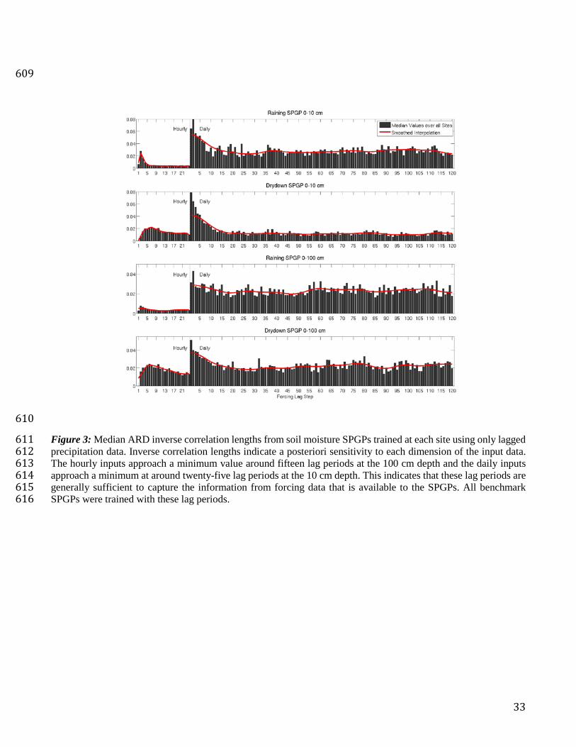
Figure 3: Median ARD inverse correlation lengths from soil moisture SPGPs trained at each site using only lagged 563

precipitation data. Inverse correlation lengths indicate a posteriori sensitivity to each dimension of the input data. 564

The hourly inputs approach a minimum value around fifteen lag periods at the 100 cm depth and the daily inputs 565

approach a minimum at around twenty-five lag periods at the 10 cm depth. This indicates that these lag periods are 566

generally sufficient to capture the information from forcing data that is available to the SPGPs. All benchmark 567

SPGPs were trained with these lag periods. 568

Figure 4: Scatterplots of soil moisture observations and estimates made by the NLDAS-2 models (black) and by 569

the benchmarks (gray) in both soil layers (top two rows for surface soil moisture; bottom two rows for top 100 cm 570

soil moisture). The ℛ𝑖𝑖u regressions (first and third rows) act on the forcing data only and the ℛu,θ regressions 571

(second and fourth rows) act on forcing data plus parameters. The mean anomaly correlations over all sites are listed 572

on each subplot. 573

27

Figure 5: The fraction of total uncertainty in soil moisture estimates contributed by each model component. These 574

plots are conceptually identical to Figure 2 except that these use real data. 575

Figure 6: Scatterplots of ET observations and estimates made by the NLDAS-2 models (black) and by the 576

benchmark estimates (grey). The ℛ𝑖𝑖u regressions (first row) act on the forcing data only and the ℛu,θ regressions 577

(second row) act on forcing data plus parameters. The mean anomaly correlations over all sites are listed on each 578

subplot. 579

580

28

Tables 581

Table 1: Parameters used by the NLDAS-2 LSMs 582 Parameter Mosaic Noah SAC-

SMA VIC

Monthly GVF(a) X X Snow-Free Albedo(a) X Monthly LAI(a) X X Vegetation Class X X X X Soil Class(b) X X X X Maximum Snow Albedo X Max/Min GVF X Average Soil Temperature X 3-Layer Porosity(c) X X 3-Layer Soil Depths X 3-Layer Bulk Density X 3-Layer Soil Density X 3-Layer Residual Moisture X 3-Layer Wilting Point(c) X X 3-layer Saturated Conductivity X Slope Type X Deep Soil Temperature(d) X X

a Linearly interpolated to the timestep. 583 b Mapped to soil hydraulic parameters. 584 c Mosaic uses a different 3-layer porosity and wilting point than VIC. 585 d Noah and VIC use different deep soil temperature values. 586 587

588

589

29

Table 2: Fractions of total uncertainty due to forcings, parameters, and structures. 590 Soil Moisture ET 10 cm 100 cm

Forcings

Noah 0.26 0.17 0.69 Mosaic 0.26 0.17 0.69 SAC-SMA 0.26 0.17 0.68 VIC 0.25 0.17 0.68

Parameters

Noah 0.53 0.52 0.20 Mosaic 0.54 0.54 0.21 SAC-SMA 0.62 0.70 0.22 VIC 0.51 0.51 0.20

Structures

Noah 0.21 0.31 0.10 Mosaic 0.20 0.29 0.11 SAC-SMA 0.12 0.14 0.10 VIC 0.24 0.32 0.11

591 592 Table 3: Efficiency of forcings, parameters and structures according to equations (2). 593

Soil Moisture ET 10 cm 100 cm

Forcings 0.77 0.85 0.40

Parameters

Noah 0.37 0.45 0.57 Mosaic 0.38 0.45 0.56 SAC-SMA 0.28 0.26 0.53 VIC 0.38 0.45 0.56

Structures

Noah 0.33 0.28 0.62 Mosaic 0.40 0.34 0.60 SAC-SMA 0.49 0.44 0.60 VIC 0.22 0.24 0.57

594

30

Figures 595

596

Figure 1: Location of the SCAN and AmeriFlux stations used in this study. Each SCAN station contributed two 597 year’s worth of hourly measurements (17,520) and each AmeriFlux station contributed four thousand hourly 598 measurements to the training of the model regressions. 599

31

600

Figure 2: A conceptual diagram of uncertainty decomposition using Shannon information. H(𝐳𝐳) represents the total 601 uncertainty (entropy) in the benchmark observations. I(𝐳𝐳;𝐮𝐮) represents the amount of information about the 602 benchmark observations that is available from the forcing data. Uncertainty due to forcing data is the difference 603 between the total entropy and the information available in the forcing data. The information in the parameters plus 604 forcing data is I(𝐳𝐳;𝐮𝐮,𝛉𝛉), and I(𝐳𝐳;𝐮𝐮,𝛉𝛉) < 𝐼𝐼(𝐳𝐳;𝐮𝐮) due to errors in the parameters. I�𝐳𝐳; 𝐲𝐲𝓜𝓜� is the total information 605 available from the model and I�𝐳𝐳; 𝐲𝐲ℳ� < 𝐼𝐼(𝐳𝐳;𝐮𝐮,𝛉𝛉) due to model structural error. This figure is adapted from (Gong 606 et al., 2013). 607

608

32

609

610

Figure 3: Median ARD inverse correlation lengths from soil moisture SPGPs trained at each site using only lagged 611 precipitation data. Inverse correlation lengths indicate a posteriori sensitivity to each dimension of the input data. 612 The hourly inputs approach a minimum value around fifteen lag periods at the 100 cm depth and the daily inputs 613 approach a minimum at around twenty-five lag periods at the 10 cm depth. This indicates that these lag periods are 614 generally sufficient to capture the information from forcing data that is available to the SPGPs. All benchmark 615 SPGPs were trained with these lag periods. 616

33

617

618

Figure 4: Scatterplots of soil moisture observations and estimates made by the NLDAS-2 models (black) and by 619 the benchmarks (gray) in both soil layers (top two rows for surface soil moisture; bottom two rows for top 100 cm 620 soil moisture). The ℛ𝑖𝑖

u regressions (first and third rows) act on the forcing data only and the ℛu,θ regressions 621 (second and fourth rows) act on forcing data plus parameters. The mean anomaly correlations over all sites are listed 622 on each subplot. 623

34

624

Figure 5: The fraction of total uncertainty in soil moisture estimates contributed by each model component. These 625 plots are conceptually identical to Figure 2 except that these use real data. 626

627

35

628

629

Figure 6: Scatterplots of ET observations and estimates made by the NLDAS-2 models (black) and by the 630 benchmark estimates (grey). The ℛ𝑖𝑖

u regressions (first row) act on the forcing data only and the ℛu,θ regressions 631 (second row) act on forcing data plus parameters. The mean anomaly correlations over all sites are listed on each 632 subplot. 633

634

635

36