Kerr black holes with synchronised scalar hair and boson stars in

the Einstein-Friedberg-Lee-Sirlin model

J. Kunz

Carl von Ossietzky University Oldenburg,

Germany Oldenburg D-26111, Germany

I. Perapechka

Department of Theoretical Physics and Astrophysics,

Belarusian State University, Minsk 220004, Belarus

Ya. Shnir

BLTP, JINR, Dubna 141980, Moscow Region, Russia

Department of Theoretical Physics, Tomsk State Pedagogical University, Russia

We consider the Friedberg-Lee-Sirlin model minimally coupled to Einstein grav-

ity in four spacetime dimensions. The renormalizable Friedberg-Lee-Sirlin model

consists of two interacting scalar fields, where the mass of the complex scalar field

results from the interaction with the real scalar field which has a finite vacuum ex-

pectation value. We here study a new family of self-gravitating axially-symmetric,

rotating boson stars in this model. In the flat space limit these boson stars tend

to the corresponding Q-balls. Subject to the usual synchronization condition, the

model admits spinning hairy black hole solutions with two different types of scalar

hair. We here investigate parity-even and parity-odd boson stars and their asso-

ciated hairy black holes. We explore the domain of existence of the solutions and

address some of their physical properties. The solutions exhibit close similarity to

the corresponding boson stars and Kerr black holes with synchronised scalar hair in

the O(3)-sigma model coupled to Einstein gravity and to the corresponding solutions

in the Einstein-Klein-Gordon theory with a complex scalar field, where the latter are

recovered in a limit.

I. INTRODUCTION

The investigation of self-gravitating scalar field configurations in 3+1 dimensional asymp-

totically flat spacetime has attracted much interest in the last decades. One of the reasons

is that a fundamental scalar field is a necessary ingredient in models of inflation. Thus such

fields might play an important role in the evolution of the early Universe. On the other

hand, when scalar fields are present in the Universe, the gravitational interaction may lead

to gravitational collapse and form localized gravitating objects. In the case of a complex

scalar field so-called boson stars might arise, that is, compact, stationary configurations

arX

iv:1

904.

1337

9v2

[gr

-qc]

9 M

ay 2

019

2

where the scalar field possesses a harmonic time dependence [1, 2].

Similar static localized field configurations with finite energy exist in Einstein-Skyrme

theory [3–5] and in SU(2) Einstein-Yang-Mills theory [6] or Einstein-Yang-Mills-Higgs the-

ory [7–10]. Certain types of localized gravitating solutions, like boson stars with appro-

priate interactions, or gravitating monopoles, sphalerons and Skyrmions, are linked to the

corresponding flat space solutions, which represent topological solitons/Q-balls [11, 12], or

monopoles [13, 14], sphalerons [15], and Skyrmions [16], respectively.

In particular, the Friedberg-Lee-Sirlin model [11] provides an interesting example of a

simple renormalizable two-component scalar field theory with natural interaction terms.

In this model the complex scalar becomes massive due to the coupling with the real scalar

field, since the latter has a finite vacuum expection value generated via a symmetry breaking

potential. The Q-ball solutions of this model then appear because of the phase rotation of

the complex scalar field, and the coupling to gravity leads to the respective boson stars.

Gravitating localized solutions of another type are bound by gravity. Examples are

boson stars without appropriate self-interactions [1, 2], or the Bartnik-McKinnon solutions

[6]. These do not possess a flat space limit.

All these self-gravitating configurations exist for a certain range of values of the pa-

rameters of the respective theory, For instance, there are two branches of self-gravitating

Skyrmions [4, 5], where the lower in energy branch is linked to the flat space Skyrmion in

the limit of a vanishing effective gravitational coupling. This lower branch of solutions then

ends at some critical maximal value of the gravitational coupling, where it bifurcates with

the second, higher in energy branch, which extends all the way backwards to the limit of zero

coupling. Likewise, for gravitating monopoles the lower in energy branch is linked to the

flat space monopole, however, the second branch ends when an extremal Reissner-Nordstrom

configuration is reached (in the exterior) [7, 8].

Boson star configurations, on the other hand, possess a presumably infinite number of

branches, representing an inspiraling of the solutions towards a limiting solution, when the

dependence of the mass or particle number on the frequency or on the radius is consid-

ered [17–20]. This spiraling behavior is reminiscent of the mass radius relation of neutron

stars beyond the maximum mass star. For other physical quantities this translates into an

oscillating behavior for boson stars and neutron stars, alike.

Notably, many of those regular particle-like gravitating solitons, like the gravitating

monopoles, sphalerons and Skyrmions or the Bartnik-McKinnon solutions, can be linked

to hairy black holes in the limit of vanishing event horizon radius [3, 21]. These static black

holes provide the first known counter-examples to the celebrated no-hair conjecture [22] (see

also [23–25] for further references and discussion).

In contrast, the spherically symmetric boson star solutions [1, 2, 17, 18] cannot be gener-

alized to contain a small Schwarzschild black hole in their inner region. More general, it has

been shown that there is no regular static asymptotically flat solution with an event horizon

in these models with a complex scalar field, which harmonically depends on time [26, 27].

3

This situation is not unique, however. For example, regular static spherically symmetric

self-gravitating solutions of the generalized Skyrme model [28, 29] terminate at a singular

solution, and cannot be continuously connected to a static hairy black hole [30].

An interesting aspect for all such gravitating regular and black hole solutions is their

possible generalization to include rotation, since rotation is ubiquitous in the Universe.

For instance, for boson stars there is no slow rotating limit [31], however, they can rotate

rapidly [32–34]. Other rotating regular configurations include the gravitating Skyrmions

and Q-clouds [35], gravitating dyons and vortex rings [36, 37] or the spinning topological

solitons of the non-linear O(3) sigma model [38].

Whereas various rotating hairy black holes were obtained before [39–44], only recently a

spinning complex scalar field was considered in a Kerr black hole spacetime, first perturba-

tively and then with back reaction [45–52]. In that case, the rotating hairy black holes obey

a synchronization condition between the angular velocity of the event horizon and a phase

frequency of the scalar field. Numerous hairy black holes obeying such a synchronization

condition have been studied by now. Further examples are given in [38, 53–63].

Interestingly, the Q-balls in the Friedberg-Lee-Sirlin model in flat space may also exist

in the limiting case of vanishing scalar potential [64, 65]. In this limit the real component

of the scalar field becomes massless, thus it possesses a Coulomb-like asymptotic tail. This

leads to the interesting question, as to whether one can find similar rotating self-gravitating

asymptotically flat solutions, which are either regular or possess an event horizon. Such

black hole solutions would represent a new type of hairy black holes, quite different from the

scalarized hairy black holes of scalar-tensor theory, where the real scalar field is associated

with the gravitational interaction [53].

In this paper we answer this question positively. In particular, we extend the study of

the spinning boson stars and hairy black holes, by constructing new families of stationary

rotating solutions in the Friedberg-Lee-Sirlin model minimally coupled to Einstein gravity.

The boson star solutions possess properties that are similar to those of the rotating boson

stars with a single complex scalar field [32–34], featuring both parity-even and parity-odd

configurations [19, 20]. In the flat space limit, they are linked to the corresponding spinning

flat-space Q-balls [19, 20, 65–68].

All these rotating boson star solutions are related to rotating hairy black hole solutions,

where the phase rotation of the massive complex component is synchronized with the angular

velocity of the horizon. An important novelty of these solutions is the fact that in the limit

of vanishing potential these solutions correspond to black holes with two different types of

scalar hair, where the second real scalar field is massless. Further, in the opposite limit

of infinite mass of the real component, the solutions of the model effectively reduce to

the corresponding boson stars and hairy black holes of the Einstein-Klein-Gordon model

[24, 46, 48, 63]. We here show that, depending on the values of the parameters of the model

and, in particular, the horizon radius parameter, the branch structure of the solutions varies

from the typical spiral pattern of boson stars [17–20, 69, 70], to a simpler branch structure

4

known for various types of hairy black holes [4, 5, 28, 29, 38–43, 46–48, 53, 53–57, 60–63, 71].

II. THE MODEL

We consider the 3+1 dimensional action

S =

∫d4x√−g(R

4α2− Lm

), (1)

where the gravity part is the usual Einstein-Hilbert action, α2 = 4πG is the gravitational

coupling, R is the curvature scalar and G is Newton’s constant. The Lagrangian of the

matter fields Lm is given by the two-component Friedberg-Lee-Sirlin model [11]

Lm =1

2(∂µψ)2 + |∂µφ|2 +m2ψ2|φ|2 − µ2

(ψ2 − v2

)2. (2)

Here a real self-interacting scalar field ψ is coupled to a complex scalar field φ, the parameters

m and µ are the real positive coupling constants and v is the vacuum expectation value of

the real scalar field ψ. The first two parts in (2) are the usual kinetic terms for the real

and complex field, respectively, the third is the interaction term, and the last term gives the

potential of the real scalar field.

The potential is chosen such that in the vacuum ψ → v, and the complex field φ becomes

massive with mass mv due to the coupling with its real partner. When expanded around

its vacuum expectation value v, the fluctuations of the real scalar field are associated with

a mass√

8µv, thus µ represents a mass parameter for the real scalar field. In the limit of

vanishing mass parameter µ→ 0 but fixed vacuum expectation value v, the real scalar field

becomes massless and thus long-ranged. The complex component φ still acquires mass in

this limit due to the coupling with the Coulomb-like field ψ.

Note that two of the four parameters of the model (1) can be rescaled away via transfor-

mations of the coordinates and the fields,

α→ vα , xµ → mvxµ , ψ → ψ

v, φ→ φ

v. (3)

After such a rescaling α = vα and µ = µ/m will be the remaining parameters. However, we

will only set v = 1 in the following, retaining α (omitting the tilde), m and µ.

The model (1) is invariant under global U(1) transformations of the complex field φ →φeδ, where the parameter δ is a constant. The following Noether current is associated with

this symmetry,

jµ = i(φ∂µφ∗ − φ∗∂µφ) , (4)

with the corresponding charge Q =∫ √−gjtd3x.

Variation of the action (1) with respect to the metric leads to the Einstein equations

Rµν −1

2Rgµν = 2α2Tµν , (5)

5

where

Tµν = ∂µψ∂νψ + (∂µφ∂νφ∗ + ∂νφ∂µφ

∗)− Lmgµν (6)

is the stress-energy tensor of the scalar fields.

The corresponding equations of motion of the scalar fields read

ψ = 2ψ(m2|φ|2 + 2µ2

(1− ψ2

)),

φ = m2ψ2φ ,(7)

where represents the covariant d’Alembert operator. It follows from the linearized field

equations (7) that the parameters µ and m indeed determine the mass of the real and

complex scalar fields, respectively. Notably, the flat-space localized regular solutions of the

Friedberg-Lee-Sirlin model (2) exist in the limit of vanishing scalar potential, µ→ 0, when

the vacuum expectation value of the real component ψ is kept non-zero [64, 65]. They

represent Q-balls with a long-range massless scalar component. These Q-balls are similar to

those of the Wick-Cutkosky model [72] revisited recently in [73, 74].

In the opposite limit, µ→∞, the real component of the model (2) trivializes, ψ = 1, and

the massive complex field φ satisfies the Klein-Gordon equation. Clearly, spatially localized

stationary spinning solutions of this equation do not exist in the flat space. However, there

are families of corresponding boson stars and hairy black holes with synchronised hair in

the complex-Klein-Gordon field theory minimally coupled to Einstein’s gravity [24, 46, 48,

61, 63].

III. SPINNING AXIALLY-SYMMETRIC CONFIGURATIONS

A. Stationary axially symmetric ansatz and boundary conditions

Spherically symmetric self-gravitating regular solutions of the equations (5),(7) do not

admit spherically symmetric generalizations with a horizon [26]. In the present paper we

shall consider spinning regular and hairy black hole solutions to the system (5),(7). We

note, that spinning self-gravitating regular solutions of an extended model with two complex

interacting scalar fields were considered before [75].

To obtain stationary spinning axially-symmetric solutions we take into account the pres-

ence of two commuting Killing vector fields ξ = ∂t and η = ∂ϕ, where t and ϕ are the time

and azimuthal coordinates, respectively. In these coordinates the metric can be written in

isotropic coordinates in the Lewis-Papapetrou form

ds2 = −F0dt2 + F1

(dr2 + r2dθ2

)+ r2 sin2 θF2

(dϕ− W

rdt

)2

, (8)

where the four metric functions F0, F1, F2 and W depend on r and θ only.

6

For the scalar fields we adopt the axially-symmetric ansatz

ψ = X(r, θ), φ = Y (r, θ)eiωt+nϕ , (9)

where the real profile functions X and Y depend on the radial coordinate r and the polar

angle θ, the frequency of the spinning complex field ω is a parameter of the model, and

n ∈ Z is the azimuthal winding number, also referred to as rotational quantum number. For

stationary spherically symmetric configurations n = 0, and the system of equations (5),(7)

reduces to the set of equations of the corresponding boson stars.

To obtain hairy black holes, we assume the existence of a rotating event horizon, located

at a constant value of the radial variable, r = rh > 0. The Killing vector of the horizon is

the helicoidal vector field

χ = ξ + Ωhη , (10)

where the horizon angular velocity Ω is fixed by the value of the metric function W on the

horizon

Ωh = −gφtgtt

∣∣∣∣r=rh

= W

∣∣∣∣r=rh

.

The presence of a rotating horizon allows to form stationary scalar clouds, supported by the

synchronisation condition [24, 38, 45, 46, 48]

ω = nΩh (11)

between the event horizon angular velocity Ωh, the complex scalar field frequency ω, and

the winding number n. This condition implies that there is no flux of the complex scalar

field into the black hole.

It is convenient to make use of the exponential parametrization of the metric fields

F0 =

(1− rh

r

)2(1 + rh

r

)2 ef0 , F1 =

(1 +

rhr

)4

ef1 , F2 =(

1 +rhr

)4

ef2 , (12)

where the functions fi depend on the radial coordinate r and the polar angle θ. Then a

power series expansion near the horizon yields the following conditions of regularity for the

profile functions X, Y and the metric functions fi:

∂rX∣∣r=rh

= ∂rY∣∣r=rh

= ∂rf0

∣∣r=rh

= ∂rf1

∣∣r=rh

= ∂rf2

∣∣r=rh

= 0 . (13)

These Neumann boundary conditions must be supplemented by the synchronization condi-

tion (11) imposed on the metric function W .

Requirement of asymptotic flatness implies that, as r → ∞, the metric approaches the

Minkowski limit, and the scalar fields are taking their vacuum values

X∣∣r→∞ = 1 , Y

∣∣r→∞ = f0

∣∣r→∞ = f1

∣∣r→∞ = f2

∣∣r→∞ = W

∣∣r→∞ = 0 . (14)

7

Demanding axial symmetry and regularity imposes the following boundary conditions on

the symmetry axis for θ = 0, π

∂θX∣∣θ=0,π

= Y∣∣θ=0,π

= ∂θf0

∣∣θ=0,π

= ∂θf1

∣∣θ=0,π

= ∂θf2

∣∣θ=0,π

= ∂θW∣∣θ=0,π

= 0 . (15)

We also require the solutions to be Z2-symmetric with respect to reflection symmetry θ →π − θ in the equatorial plane θ = π/2. Thus, we can restrict the range of values of the

angular variable as θ ∈ [0, π/2]. The corresponding boundary conditions on the equatorial

plane are

∂θX∣∣θ=π

2

= ∂θf0

∣∣θ=π

2

= ∂θf1

∣∣θ=π

2

= ∂θf2

∣∣θ=π

2

= ∂θW∣∣θ=π

2

= 0 . (16)

0.3 0.4 0.5 0.6 0.7 0.8 0.9 1.00

10

20

30

40

50

=0

Mm

/m

=0.25

0 20 40 60 80 1000

10

20

30

40

50

=0.25Mm

Qm2

=0

FIG. 1: The ADM mass M vs the angular frequency ω (left plot) and Noether charge Q (right

plot) at µ/m = 0.25, µ = 0 and α = 0.5 for parity-even boson stars.

Further, there are two different types of axially symmetric solutions, which possess differ-

ent parity of the complex scalar field [19, 20, 65]. The corresponding boundary conditions on

the complex component of the field in the equatorial plane are ∂θY∣∣θ=π

2

= 0 for parity-even

solutions, and Y∣∣θ=π

2

= 0 for parity-odd configurations.

Note that the absence of a conical singularity on the symmetry axis requires that the

deficit angle should vanish, δ = 2π(

1− limθ→0

F2

F1

)= 0. Hence the solutions should satisfy the

constraint F2

∣∣θ=0

= F1

∣∣θ=0

. In our numerical scheme we explicitly checked this condition on

the symmetry axis.

B. Quantities of interest and Smarr relation

Asymptotic expansions of the metric functions at the horizon and at spatial infinity yield

a number of physical observables. The total ADM mass M and the angular momentum J

8

Kerr

rh=0.06

rh=0.05rh=0.04rh=0.03

rh=0.02

rh=0.01

rh=0Mm

/m

rh=0

rh=0.06

rh=0.05rh=0.04

rh=0.03

rh=0.02

rh=0.01

Kerr

Mm

/m

0.60 0.65 0.70 0.75 0.80 0.85 0.90 0.95 1.000.01

0.1

0.5

1

2

rh=0.06

rh=0.05

rh=0.04

rh=0.03

rh=0.02

r h=0.01

T H/m

/m0.65 0.70 0.75 0.80 0.85 0.90 0.95 1.00

0.01

0.1

0.5

1

2

rh=0.06rh=0.0

5

rh=0.04

rh=0.03

rh=0.02

r h=0.01

T H/m

/m

0 10 20 30 40 50 60 700

10

20

30

40

50

60

70

rh=0.03

rh=0.02rh=0.01

rh=0

Mm

Jm2

0 10 20 30 40 50 60 70 80 900

10

20

30

40

50

60

70

80

90

rh=0 rh=0.01 rh=0.02 rh=0.03

Mm

Jm2

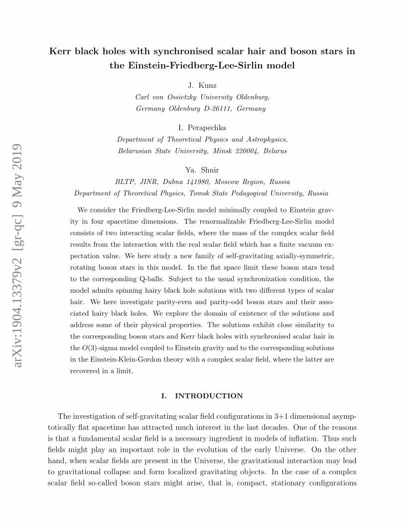
FIG. 2: The ADM mass M (upper row) and the Hawking temperature Th (middle row) vs the

frequency ω, and the mass M vs the angular momentum J (bottom row) for a set of values of

the horizon radius parameter rh for n = 1 rotating parity-even (left column) and parity-odd (right

column) hairy black holes at µ/m = 0.25 and α = 0.5. In the left plots, here, and in the subsequent

figures below, the shaded area corresponds to the domain of existence of vacuum Kerr black holes,

the red dashed line to the extremal vacuum Kerr black holes, and the blue dashed line to the subset

of vacuum Kerr black holes with stationary scalar Klein-Gordon clouds.

9

0.60 0.65 0.70 0.75 0.80 0.85 0.90 0.95 1.000.8

0.9

0.95

0.99

1

rh=0.06

rh=0.05

rh=0.04

rh=0.03

rh=0.02

rh=0.01

X(r h)

/m0.60 0.65 0.70 0.75 0.80 0.85 0.90 0.95 1.000

0.01

0.1

0.2

0.4

rh=0.06

rh=0.05

rh=0.04rh=0.03

rh=0.02

rh=0.01

Y max(r h

)

/m

0.65 0.70 0.75 0.80 0.85 0.90 0.95 1.000.9

0.95

0.99

0.999

1rh=0.06

rh=0.05

rh=0.04

rh=0.03

rh=0.02

rh=0.01

X(r h)

/m0.65 0.70 0.75 0.80 0.85 0.90 0.95 1.000

0.0001

0.001

0.01

0.02

rh=0.06

rh=0.05

rh=0.04

rh=0.03

rh=0.02

rh=0.01

Y max(r h

)

/m

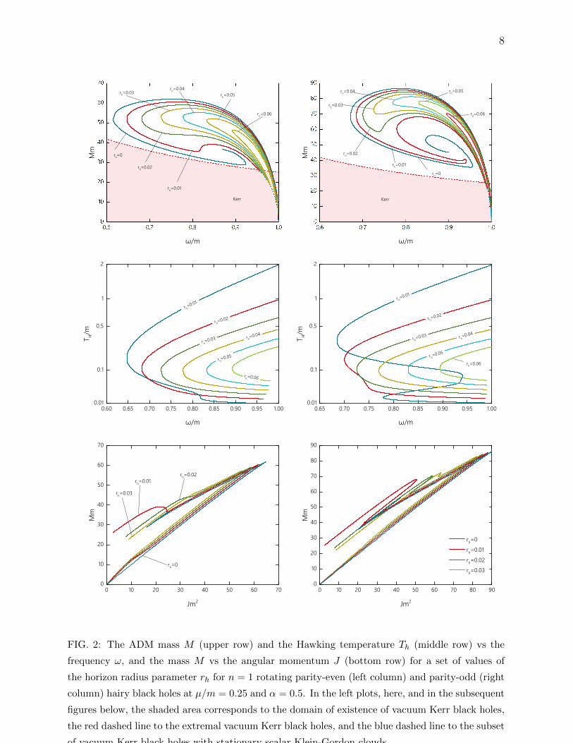
FIG. 3: The value of real scalar field on the horizon X(rh) at θ = 0 (left column) and the maximal

value of the complex scalar field on the horizon Ymax(rh) (left column) vs the frequency ω for a

set of values of the horizon radius parameter rh for n = 1 rotating parity-even (upper row) and

parity-odd (lower row) hairy black holes at µ/m = 0.25 and α = 0.5.

of the spinning hairy black holes can be read off from the asymptotic subleading behaviour

of the metric functions as r →∞

gtt = −1 +α2M

πr+O

(1

r2

), gϕt =

α2J

πrsin2 θ +O

(1

r2

). (17)

The ADM charges can be represented as sums of the contributions from the event horizon

and the scalar hair, M = Mh +MΦ and J = Jh + JΦ, respectively. These contributions can

10

0.0 0.1 0.2 0.3 0.4 0.5 0.6 0.7 0.8 0.9 1.0

5

10

50

100

500

rh=0, =0.25

rh=0.05, =0.25

rh=0.01, =0.25

rh=0.01, =0

Mm

FIG. 4: The scalar hair mass MΦ vs the gravitational coupling constant α for a set of values of

horizon radius parameter rh and the potential coupling constant µ for n = 1 rotating parity-even

hairy black holes at frequency ω/m = 0.9.

be evaluated separately via Komar integrals

Mh = − 1

2α2

∮S

dSµν∇µξν , Jh =1

4α2

∮S

dSµν∇µην ,

MΦ = − 1

α2

∫V

dSµ (2T µν ξν − Tξµ), JΦ =

1

2α2

∫V

dSµ

(T µν η

ν − 1

2Tηµ

),

(18)

where S is the horizon 2-sphere and V denotes an asymptotically flat spacelike hypersurface

bounded by the horizon.

Analogously to other axially symmetric stationary rotating boson stars [19, 20], self-

gravitating solitons of the non-linear sigma model [38] and vortons [75], one obtains the

quantization relation for the angular momentum of the spinning complex scalar component

of the model, JΦ = nQ, where Q is its Noether charge and n its winding number.

The physically interesting horizon properties include the Hawking temperature Th, which

is proportional to the surface gravity κ2 = −12∇µχν∇µχν

Th =κ

2π=

1

16πrhexp

[(f0 − f1)

∣∣r=rh

], (19)

11

FIG. 5: Contour plots of the profile function of the real scalar field X (first and third columns)

and the profile function of the complex scalar field Y (second and fourth columns) in the y = 0

plane for parity-even (left two columns) and parity-odd (right two columns) n = 1 black holes with

synchronized hair at ω/m = 0.9, α = 0.5 and horizon radius parameter rh = 0.05. The upper row

shows solutions for a finite value of the real scalar field mass µ/m = 0.25, whilst the bottom row

shows solutions for a massless real scalar field with µ = 0.

where χ is the horizon Killing vector (10). Of interest is also the horizon area Ah, which is

given by

Ah = 32πr2h

∫ π

0

dθ sin θ exp[(f1 + f2)

∣∣r=rh

]. (20)

The observables are related via the Smarr relation

M = 2ThS + 2ΩhJh +MΦ , (21)

where S = πα2Ah is the entropy of the black hole and MΦ is the energy of the scalar fields

outside the event horizon (18). Another relation between the physical quantities of the hairy

12

Kerr

rh=0.04

rh=0.01

rh=0

M

/m0.1 0.2 0.3 0.4 0.5 0.6 0.7 0.8 0.9 1.0

0.001

0.01

0.1

0.5

1

2

rh=0.06rh=0.05

rh=0.04rh=0.03

rh=0.02

rh=0.01

T H/m

/m

FIG. 6: The ADM mass M (left plot) and the Hawking temperature Th (right plot) vs the frequency

ω for a set of values of the horizon radius parameter rh for n = 1 rotating parity-even hairy black

holes in the limiting case of vanishing scalar potential (µ = 0) at α = 0.5. To simplify the

presentation the ADM mass is multiplied by ω.

black hole is the first law of thermodynamics

dM = ThdS + ΩhdJ .

IV. RESULTS

A. Numerical implementation

The set of six coupled non-linear elliptic partial differential equations of the functions

X, Y,W, f0, f1, f2, which parametrize the system (5),(7), has been solved numerically subject

to the boundary conditions (13)-(15). We have made use of a fourth-order finite differences

scheme, where the system of equations is discretized on a grid with 101 × 101 points. To

facilitate the calculations in the near horizon area, we have introduced the new radial coordi-

nate x = r−rhr+c

, which maps the semi-infinite region [0,∞) onto the unit interval [0, 1]. Here

c is an arbitrary constant used to adjust the contraction of the grid. The emerging system

of nonlinear algebraic equations is solved using a modified Newton method. The underlying

linear system is solved with the Intel MKL PARDISO sparse direct solver. The errors are

on the order of 10−5. All calculation have been performed using CESDSOL 1 library.

1 Complex Equations – Simple Domain partial differential equations SOLver is a C++ library developed

by IP. It provides tools for the discretization of an arbitrary number of arbitrarily nonlinear equations

13

Kerr

even-parity odd-parity

M

/m

0.10 0.15 0.20 0.2538

40

42

44

0.05 0.10 0.15 0.2029

30

31

32

33

0.85 0.90

34

36

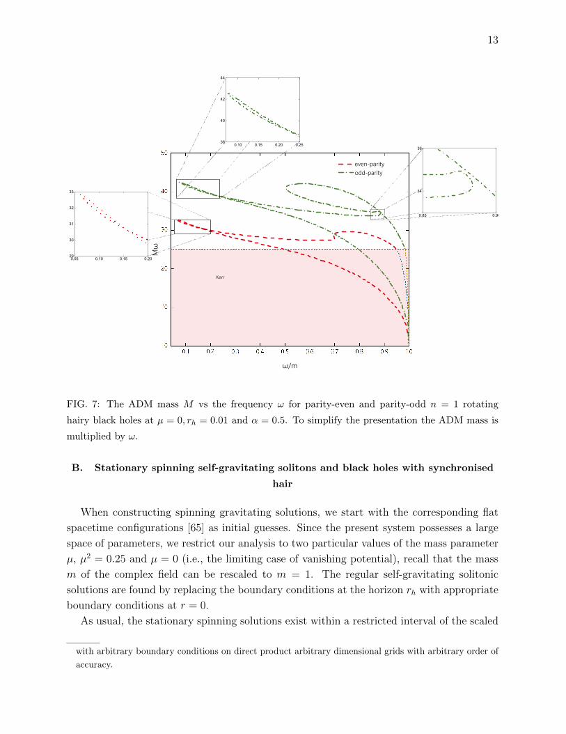
FIG. 7: The ADM mass M vs the frequency ω for parity-even and parity-odd n = 1 rotating

hairy black holes at µ = 0, rh = 0.01 and α = 0.5. To simplify the presentation the ADM mass is

multiplied by ω.

B. Stationary spinning self-gravitating solitons and black holes with synchronised

hair

When constructing spinning gravitating solutions, we start with the corresponding flat

spacetime configurations [65] as initial guesses. Since the present system possesses a large

space of parameters, we restrict our analysis to two particular values of the mass parameter

µ, µ2 = 0.25 and µ = 0 (i.e., the limiting case of vanishing potential), recall that the mass

m of the complex field can be rescaled to m = 1. The regular self-gravitating solitonic

solutions are found by replacing the boundary conditions at the horizon rh with appropriate

boundary conditions at r = 0.

As usual, the stationary spinning solutions exist within a restricted interval of the scaled

with arbitrary boundary conditions on direct product arbitrary dimensional grids with arbitrary order of

accuracy.

14

=0.25=0.01=0.001

=0M

/m0.0 0.1 0.2 0.3 0.4 0.5 0.6 0.7 0.8 0.9 1.0

0.001

0.01

0.1

0.5

1

2

=0.25=0.01=0.0

01

=0

T H/m

/m

=0.25

=0.01

=0

M

/m0.0 0.1 0.2 0.3 0.4 0.5 0.6 0.7 0.8 0.9 1.0

0.001

0.01

0.1

0.5

1

2

=0.25

=0.01=0.

001

=0T H/m

/m

FIG. 8: The ADM mass M (left column) and the Hawking temperature Th (right column) vs

the frequency ω for a set of values of the potential coupling constant µ/m for n = 1 parity-even

(upper row) and parity-odd (lower row) rotating hairy black holes at the horizon radius parameter

rh = 0.01 and α = 0.5.

frequency ω ∈ [ωmin, ωmax = 1]. The upper bound of the frequency ω corresponds to the

mass of the complex scalar field, the lower critical frequency depends on the value of the

second mass parameter µ. As ω → ωmax = 1 the spinning configurations smoothly approach

linearized perturbations around Minkowski spacetime, with the ADM mass M tending to

zero.

Note that, unlike the corresponding solutions of the non-renormalizable flat space model

with a single complex field and a sextic potential [19, 20], there is no lower bound on the

frequency in the flat space limit of the present model: the Friedberg-Lee-Sirlin Q-balls exist

for all non-zero values of the frequency ω < m [64, 65]. As we shall see, the coupling to

gravity changes this, and a lower critical value of the frequency appears.

15

Setting the winding number n to n = 0 reduces the above system to the spherically

symmetric case of the regular boson star solutions. In Fig. 1 we display the ADM mass M

as a function of rescaled frequency (left) and the mass M vs the charge Q for oscillating

n = 0 parity-even boson stars in the model (1).

Notably, the coupling to gravity reduces the interval of values of the frequency ω, and

the spherically symmetric boson stars exist in a more limited frequency range. The minimal

value ωmin > 0 depends on the strength of the gravitational coupling α and on the value

of the mass parameter µ, see Fig. 1, left plot. As expected, these boson stars exhibit a

typical spiral-like frequency dependence of the charge and the mass, and should approach

finite limiting values at the centers of the spirals.

Considering the n = 0 configurations we do not find spherically symmetric hairy black

holes, as expected. However, taking n ≥ 1, we obtain both boson stars with non-zero

angular momentum, and spinning hairy black holes. Furthermore, for n ≥ 1 there are two

different types of spinning configurations, [19, 20, 61, 63, 66], referred to as parity-even and

parity-odd solutions, respectively.

In Fig. 2 the ADM mass M of the n = 1 parity-even and parity-odd solutions is exhibited

versus the frequency ω for a set of values of the horizon radius parameter rh, including the

regular limit rh = 0, for the chosen values of the mass parameter µ2 = 0.25 and the gravita-

tional coupling α = 0.5. The families of boson star solutions are found in the rh → 0 limit.

They emerge from the vacuum at ωmax = 1, and form the fundamental branch of solutions.

Both the dependence of the mass and the Noether charge of the regular configurations on

the frequency form an inspiraling pattern, which is typical for spinning boson star solutions

and some other types of gravitating solitons [19, 20, 38, 53, 75].

As the fundamental branch of regular solutions arises from the upper limiting frequency

value ωmax, the mass M of the configurations gradually increases with decreasing ω and, for

all values of the mass parameter µ not too close to zero, the dependence M(ω) possesses

a maximum at some critical value of the frequency ωM. As the frequency decreases below

that point, the mass of the solutions decreases until the minimum frequency ωmin is reached.

Here the fundamental forward branch merges with a second (backward) branch, leading to

a counterclockwise inspiraling of the mass curve M(ω).

In general, for the same set of values of the parameters of the model, the mass of the

parity-odd configurations is considerably higher than the mass of the parity-even boson

stars, as seen in Fig. 2, left column. The parity-odd n = 1 solutions represent a new family

of boson stars, which in the flat space limit are linked to the corresponding Q-balls [65].

We have found that black holes with synchronized hair exist in a small interval of the

event horizon radius parameter, typically rh < 0.07, see Fig. 2. For very small values of

the horizon radius rh, rh < 0.02, the inspiraling critical behavior is changed to a multi-

branch structure with a few branches only, leading toward a second upper critical value

of the frequency ω(1)cr < 1, see Fig. 2, left plots. In this limit, the real scalar component

trivializes and the lower branch ends on the vacuum Kerr black holes with stationary scalar

16

Klein-Gordon clouds, see [24, 38, 45, 46, 48, 54].

As the horizon radius rh increases, the multibranch structure is replaced by a two-branch

scenario with the second (lower, backward) branch ending on the limiting Kerr solution as

ω → ω(1)cr , see Fig. 2, left column. The maximum value of the frequency along the second

branch ω(1)cr slowly increases as the horizon radius rh grows, and approaches ωmax = 1 at

some maximal value of the horizon radius rh as the loop shrinks to zero. The branches exist

up to the limit α = 0, where the regular solutions approach the corresponding flat space

Q-ball configurations while the solutions with non-zero horizon radius rh become linked to

the scalar clouds spinning around the Kerr black hole in the probe limit.

The Hawking temperature constantly decreases as ω varies along the branches, see Fig. 2,

middle column. Note that the configurations with the smallest horizon radius rh have the

smallest temperature, both for the parity-even and parity-odd solutions.

Fig. 2 also presents the ADM mass as a function of the angular momentum J , see the

right column. The mass of the regular spinning configurations with horizon radius rh = 0

exhibits a typical zig-zag behavior known for boson stars [17–20, 53, 68, 70]. As the horizon

radius increases, it becomes replaced with the two-branch pattern, which is well known for

the Kerr scalar clouds and other similar solutions [24, 38, 45, 46, 48, 54]. Here the lower

branch corresponds to the values of the frequency smaller than ω(1)cr , while the upper branch

represents the values ω > ω(1)cr .

In Fig. 3 we present the horizon values of the massive scalar fields X(rh and Y (rh) as

functions of the frequency ω for µ2 = 0.25. Both the parity-even and the parity-odd solutions

start at ωmax = 1 from the regular limits X(ωmax) = 1, Y (ωmax) = 0.

To conclude the analysis of the massive (µ2 = 0.25) spinning configurations, we exhibit

in Fig. 4 the dependence of the scalar mass of the n = 1 parity-even solutions on the

gravitational coupling α for some set of the values of the horizon radius rh. One can see

that the mass of the solutions on both branches decreases monotonically as α increases. In

the limiting case α → 0 the solutions approach the Q-balls spinning on the Minkowski or

Schwarzschild background.

The situation changes drastically for the spinning solutions when µ → 0. First, we

observe that the spinning component of the coupled configuration falls off exponentially. It

remains massive, whereas the real scalar field decays as ∼ r−1. Fig. 5 exhibits the profile

functions of both parity-even and parity-odd scalar field functions X(r, θ) and Y (r, θ) for the

massive µ2 = 0.25 and the massless (µ = 0) case. Thus, the massless limit provides a new

type of hairy black hole with hair of two different types, that are short- and long-ranged,

respectively.

In Fig. 6 we display the ADM mass M (left column) and the Hawking temperature TH(middle column) of the parity-even n = 1 configurations versus the frequency ω. Similar

to the solutions with non-zero values of the mass parameter µ presented in Fig. 2, the

fundamental branch of the regular spinning boson stars arises in the limit ωmax = 1, and the

mass of the configuration increases as the frequency decreases. This branch extends up to

17

some lower non-zero critical value ωmin > 0, and the ADM mass of the boson star increases

monotonically along this branch.

The lower critical value ωmin depends on the strength of the gravitational coupling, and

increases slowly as α grows. In the flat space limit the axially-symmetric spinning Q-balls

with massless real component exist over the entire range of values of the frequency ω ∈ [0, 1]

[64, 65]. We constructed solutions with very large values of α, and they are likely to exist

for arbitrary values of the effective gravitational coupling.

FIG. 9: Ergosurfaces of n = 1 parity-even hairy BHs with horizon radius parameter rh = 0.01

and frequencies ω/m = 0.35 (1), ω/m = 0.5 (2) and parity-odd BH with ω/m = 0.5 (3) on the

backward branch. Blue surfaces represent the horizon.

This branch bifurcates with the second upper branch at ωmin, and we observe a small loop

in the M(ω) dependence, as illustrated in Fig. 6, left plot, see also the zoomed-in subplot

in Fig. 7. This loop, which is observed both for the parity-even and parity-odd black holes

with a synchronized massive component, disappears when the mass parameter µ increases

sufficiently from zero.

The mass of the configurations rapidly increases as the frequency ω approaches its minimal

value ωmin. Further increase of the frequency ω along the second branch is related with a

decrease of the mass. At some upper critical value of the frequency ω(2)cr the curve backbends

and a third (backward) branch of the regular spinning solitons is found. Thus, an overall

inspiral type pattern is observed again for this sequence of solutions.

We have performed a similar study also for the parity-odd µ = 0 solutions with a long-

range real component, see Fig. 7. The branch structure of the spinning parity-odd black

holes with synchronized hair is more explicit than the one of the corresponding parity-even

solutions. In particular, for small values of the horizon radius, the third and the forth branch

are clearly visible.

In addition, Fig. 8 exhibits the pattern of the evolution of the branches of the parity-even

(upper row) and parity-odd (bottom row) solutions at the horizon radius rh = 0.01, as the

mass parameter µ varies. We observe that the range of allowed values of the frequency

18

rapidly decreases as µ grows. In the limiting case, µ → ∞, the real scalar component

becomes trivial everywhere in space, so the model (1) becomes effectively truncated to the

massive complex-Klein-Gordon theory minimally coupled to Einstein gravity [76].

It is known, that the latter model supports the existence of black holes with synchronised

hair [45, 46, 48]. These solutions trivialize when the gravitational coupling is switched off.

Indeed, our simulations show that the spinning component of the parity-even solutions of

the model (1) approaches the corresponding solutions of the complex-Klein-Gordon theory

presented in [46, 48]. On the other hand, in the limit µ→∞ the n = 1 parity-odd solutions

of the model (2) approach Kerr black holes with parity-odd synchronised scalar hair [61, 63].

Finally, we address the geometry of the ergo-surfaces of the hairy black holes in the

Einstein-Friedberg-Lee-Sirlin model. The ergo-surfaces are defined as the zero locus of the

normalized time-like Killing vector ξ · ξ = 0, or

gtt = −F0 + sin2 θF2W2 = 0 . (22)

We found that, in analogy to other known hairy black holes, there are both the ordinary

Kerr-like S2 ergo-regions with topology S2, which appear on the fundamental branch, and

ergo-Saturns with topology S2⊕

(S1 × S1), when the black holes possess parity-even scalar

hair [47, 53], see Fig. 9. Further, analogously to the corresponding parity-odd solutions in

the Einstein-Klein-Gordon theory [63], there is a new type of ergo-surfaces, which represent

ergo-double-torus-Saturns with topology (S1 × S1)⊕

(S1 × S1)⊕

S2, see Fig. 9, right plot.

n=2

n=4

n=3

Kerr

n=1

Mm

/m0.5 0.6 0.7 0.8 0.9 1.0

0.00

0.05

0.10

0.15

0.20

0.25

0.30

0.35

0.40

n=4

n=3

n=2

n=1

T H/m

/m

FIG. 10: The ADM mass M (left plot) and the Hawking temperature Th (right plot) vs the

frequency ω/m for a set of values of the winding number n for rotating parity-even hairy black

holes at the horizon radius rh = 0.05 and µ/m = 0.25.

Also, we constructed spinning solutions for higher values of the azimuthal winding number

n > 1. Generally, these possess similar properties as the n = 1 solutions, however, their

19

mass is higher, and they exist in a larger interval of frequencies, as seen in Fig. 10.

V. CONCLUSIONS

In this work we have coupled the Friedberg-Lee-Sirlin model [11] to Einstein gravity

and investigated some of its solutions. When the flat space non-topological solitons are

coupled to gravity, regular boson star solutions arise. In the simplest case, these boson star

solutions are spherically symmetric. Here, however, we have concentrated on their rotating

generalizations, which may feature a parity-even or parity-odd complex scalar field.

The properties of these boson stars are similar to those found in models with a complex

scalar field only, like the Einstein-Klein-Gordon model. In fact the solutions of this model

are recovered, when the coupling constant µ is taken to infinity. On the other hand, also

boson star solutions with a massless real scalar field have been found.

When the presence of an event horizon together with the synchronization condition be-

tween the frequency and the horizon angular velocity is imposed, new hairy black holes

emerge in a certain region of the parameter space. According to the symmetries of the

complex scalar field they represent parity-even or parity-odd hairy black holes.

These hairy black holes possess two types of hair, consisting of the usual complex scalar

field hair and the additional real scalar field hair. In particular, when the mass of the real

scalar field vanishes, the real scalar field hair becomes long-ranged, whereas the complex

scalar field hair remains massive. This constitutes an interesting new quality of hairy black

holes.

We note that similar hairy black hole solutions as the ones studied here may also exist

in the Wick-Cutkosky model [72], recently revisited in [73, 74], if the corresponding Q-ball

configurations are coupled to Einstein gravity.

Various interesting features of the regular and hairy black hole solutions of the Einstein-

Friedberg-Lee-Sirlin model remain to be studied, and, in particular, there should be nu-

merous further radially and angularly excited regular and hairy black hole solutions in the

model.

Acknowledgements– We are grateful to Burkhard Kleihaus and Eugen Radu for inspir-

ing and valuable discussions. This work was supported in part by the DFG Research Training

Group 1620 Models of Gravity as well as by and the COST Action CA16104 GWverse. Ya.S.

gratefully acknowledges the support of the Alexander von Humboldt Foundation and from

the Ministry of Education and Science of Russian Federation, project No 3.1386.2017. I.P.

would like to acknowledge support by the DAAD Ostpartnerschaft Programm.

[1] D. J. Kaup, Phys. Rev. 172 (1968) 1331.

[2] R. Ruffini and S. Bonazzola, Phys. Rev. 187 (1969) 1767.

20

[3] H. Luckock and I. Moss, Phys. Lett. B 176 (1986) 341.

[4] S. Droz, M. Heusler and N. Straumann, Phys. Lett. B 268 (1991) 371.

[5] P. Bizon and T. Chmaj, Phys. Lett. B 297 (1992) 55.

[6] R. Bartnik and J. Mckinnon, Phys. Rev. Lett. 61 (1988) 141.

[7] K. M. Lee, V. P. Nair and E. J. Weinberg, Phys. Rev. D 45, 2751 (1992)

[8] P. Breitenlohner, P. Forgacs and D. Maison, Nucl. Phys. B 383, 357 (1992)

[9] B. R. Greene, S. D. Mathur and C. M. O’Neill, Phys. Rev. D 47, 2242 (1993)

[10] P. Breitenlohner, P. Forgacs and D. Maison, Nucl. Phys. B 442, 126 (1995)

[11] R. Friedberg, T. D. Lee and A. Sirlin, Phys. Rev. D 13 (1976) 2739

[12] S. R. Coleman, Nucl. Phys. B 262 (1985) 263 Erratum: [Nucl. Phys. B 269 (1986) 744].

[13] G. ’t Hooft, Nucl. Phys. B 79, 276 (1974).

[14] A. M. Polyakov, JETP Lett. 20, 194 (1974) [Pisma Zh. Eksp. Teor. Fiz. 20, 430 (1974)].

[15]

[15] F. R. Klinkhamer and N. S. Manton, Phys. Rev. D 30, 2212 (1984).

[16] T. H. R. Skyrme, Proc. Roy. Soc. Lond. A 260 (1961) 127.

[17] R. Friedberg, T. D. Lee and Y. Pang, Phys. Rev. D 35 (1987) 3640

[18] R. Friedberg, T. D. Lee and Y. Pang, Phys. Rev. D 35, 3658 (1987).

[19] B. Kleihaus, J. Kunz and M. List, Phys. Rev. D 72 (2005) 064002

[20] B. Kleihaus, J. Kunz, M. List and I. Schaffer, Phys. Rev. D 77 (2008) 064025

[21] M. S. Volkov and D. V. Galtsov, JETP Lett. 50 (1989) 346 [Pisma Zh. Eksp. Teor. Fiz. 50

(1989) 312];

[22] R. Ruffini and J. A. Wheeler, Phys. Today 24 (1971) no.1, 30

[23] M. S. Volkov and D. V. Gal’tsov, Phys. Rept. 319, 1 (1999)

[24] C. A. R. Herdeiro and E. Radu, Int. J. Mod. Phys. D 24 (2015) no.09, 1542014

[25] M. S. Volkov, arXiv:1601.08230 [gr-qc].

[26] I. Pena and D. Sudarsky, Class. Quant. Grav. 14 (1997) 3131.

[27] S. Hod, Phys. Lett. B 778 (2018) 239.

[28] C. Adam, O. Kichakova, Y. Shnir and A. Wereszczynski, Phys. Rev. D 94 (2016) no.2, 024060

[29] S. B. Gudnason, M. Nitta and N. Sawado, JHEP 1609 (2016) 055

[30] I. Perapechka and Y. Shnir, Phys. Rev. D 95 (2017) no.2, 025024

[31] Y. Kobayashi, M. Kasai and T. Futamase, Phys. Rev. D 50, 7721 (1994).

[32] F. E. Schunck and E. W. Mielke, Phys. Lett. A 249, 389 (1998).

[33] F. D. Ryan, Phys. Rev. D 55, 6081 (1997).

[34] S. Yoshida and Y. Eriguchi, Phys. Rev. D 56, 762 (1997).

[35] T. Ioannidou, B. Kleihaus and J. Kunz, Phys. Lett. B 643 (2006) 213

[36] B. Kleihaus, J. Kunz and U. Neemann, Phys. Lett. B 623, 171 (2005)

[37] B. Kleihaus, J. Kunz, F. Navarro-Lerida and U. Neemann, Gen. Rel. Grav. 40, 1279 (2008)

[38] C. Herdeiro, I. Perapechka, E. Radu and Y. Shnir, JHEP 1902 (2019) 111

21

[39] B. Kleihaus and J. Kunz, Phys. Rev. Lett. 86, 3704 (2001)

[40] B. Kleihaus, J. Kunz and F. Navarro-Lerida, Phys. Rev. D 66, 104001 (2002)

[41] B. Kleihaus, J. Kunz and F. Navarro-Lerida, Phys. Rev. D 69, 064028 (2004)

[42] B. Kleihaus, J. Kunz and F. Navarro-Lerida, Phys. Rev. D 69, 081501 (2004)

[43] B. Kleihaus, J. Kunz and F. Navarro-Lerida, Phys. Lett. B 599, 294 (2004)

[44] B. Kleihaus, J. Kunz and F. Navarro-Lerida, Class. Quant. Grav. 33, no. 23, 234002 (2016)

[45] S. Hod, Phys. Rev. D 86 (2012) 104026 Erratum: [Phys. Rev. D 86 (2012) 129902]

[46] C. A. R. Herdeiro and E. Radu, Phys. Rev. Lett. 112 (2014) 221101

[47] C. Herdeiro and E. Radu, Phys. Rev. D 89 (2014) no.12, 124018

[48] C. Herdeiro and E. Radu, Class. Quant. Grav. 32 (2015) no.14, 144001

[49] S. Hod, Phys. Rev. D 90 (2014) no.2, 024051

[50] C. L. Benone, L. C. B. Crispino, C. Herdeiro and E. Radu, Phys. Rev. D 90, no. 10, 104024

(2014)

[51] C. Herdeiro, E. Radu and H. Runarsson, Phys. Lett. B 739 (2014) 302

[52] C. A. R. Herdeiro and E. Radu, Int. J. Mod. Phys. D 23 (2014) no.12, 1442014

[53] B. Kleihaus, J. Kunz and S. Yazadjiev, Phys. Lett. B 744 (2015) 406

[54] C. A. R. Herdeiro, E. Radu and H. Runarsson, Phys. Rev. D 92 (2015) no.8, 084059

[55] C. Herdeiro, J. Kunz, E. Radu and B. Subagyo, Phys. Lett. B 748, 30 (2015)

[56] C. Herdeiro, E. Radu and H. Runarsson, Class. Quant. Grav. 33 (2016) no.15, 154001

[57] Y. Brihaye, C. Herdeiro and E. Radu, Phys. Lett. B 760 (2016) 279

[58] S. Hod, Phys. Lett. B 751 (2015) 177

[59] C. Herdeiro, J. Kunz, E. Radu and B. Subagyo, Phys. Lett. B 779, 151 (2018)

[60] C. Herdeiro, I. Perapechka, E. Radu and Y. Shnir, JHEP 1810 (2018) 119

[61] Y. Q. Wang, Y. X. Liu and S. W. Wei, Phys. Rev. D 99 (2019) no.6, 064036

[62] J. F. M. Delgado, C. A. R. Herdeiro and E. Radu, arXiv:1903.01488 [gr-qc].

[63] J. Kunz, I. Perapechka and Y. Shnir, arXiv:1904.07630 [gr-qc].

[64] A. Levin and V. Rubakov, Mod. Phys. Lett. A 26 (2011) 409.

[65] V. Loiko, I. Perapechka and Y. Shnir, Phys. Rev. D 98 (2018) no.4, 045018

[66] M.S. Volkov and E. Wohnert, Phys. Rev. D 66 (2002) 085003.

[67] E. Radu and M.S. Volkov, Phys. Rept. 468 (2008) 101.

[68] Y. Brihaye and B. Hartmann, Phys. Rev. D 79 (2009) 064013

[69] T. Tamaki and N. Sakai, Phys. Rev. D 81 (2010) 124041

[70] L. G. Collodel, B. Kleihaus and J. Kunz, Phys. Rev. D 96 (2017) no.8, 084066

[71] I. Perapechka and Y. Shnir, Phys. Rev. D 96 (2017) no.12, 125006

[72] G. C. Wick, Phys. Rev. 96 (1954) 1124;

R. E. Cutkosky, Phys. Rev. 96 (1954) 1135.

[73] E. Y. Nugaev and M. N. Smolyakov, Eur. Phys. J. C 77 (2017) no.2, 118

[74] A. G. Panin and M. N. Smolyakov, Eur. Phys. J. C 79 (2019) no.2, 150

22

[75] J. Kunz, E. Radu and B. Subagyo, Phys. Rev. D 87 (2013) no.10, 104022

[76] F. E. Schunck and E. W. Mielke, Class. Quant. Grav. 20 (2003) R301