Embed Size (px)
Citation preview

BEC in Optical Lattices: Beyond theBogoliubov Approximation
Diploma Thesis by
Pascal Mattern
Supervisor: Prof. Dr. Dr. h.c. mult. Hagen Kleinert
submitted to the
Faculty of PhysicsFreie Universitat Berlin
May 2012

2

Contents
1 Introduction 1
1.1 What is a BEC? . . . . . . . . . . . . . . . . . . . . . . . . . . . . . . . . . . . . 1
1.2 Why are BEC’s interesting? . . . . . . . . . . . . . . . . . . . . . . . . . . . . . 2
1.3 Overview of this diploma thesis . . . . . . . . . . . . . . . . . . . . . . . . . . . 3
2 BEC in optical lattices 5
2.1 Theoretical basics . . . . . . . . . . . . . . . . . . . . . . . . . . . . . . . . . . . 5
2.1.1 Bose-Hubbard-Hamiltonian . . . . . . . . . . . . . . . . . . . . . . . . . 5
2.1.2 Phase transitions . . . . . . . . . . . . . . . . . . . . . . . . . . . . . . . 8
2.2 Experimental realization . . . . . . . . . . . . . . . . . . . . . . . . . . . . . . . 9
3 Effective Hamiltonian for the Bogoliubov Approximation 15
3.1 Bogoliubov Approximation . . . . . . . . . . . . . . . . . . . . . . . . . . . . . . 15
3.2 The condensate density . . . . . . . . . . . . . . . . . . . . . . . . . . . . . . . . 22
3.3 The grand-canonical potential and self-consistency . . . . . . . . . . . . . . . . . 23
3.4 Plots for T = 0 . . . . . . . . . . . . . . . . . . . . . . . . . . . . . . . . . . . . 26
3.5 Popov approximation . . . . . . . . . . . . . . . . . . . . . . . . . . . . . . . . . 27
4 Beyond the Bogoliubov approximation: second order 33
4.1 How perturbation theory for T 6= 0 works . . . . . . . . . . . . . . . . . . . . . . 33
4.2 The Wick theorem . . . . . . . . . . . . . . . . . . . . . . . . . . . . . . . . . . 34
4.3 Beyond Bogoliubov . . . . . . . . . . . . . . . . . . . . . . . . . . . . . . . . . . 36
4.4 The H(4) term . . . . . . . . . . . . . . . . . . . . . . . . . . . . . . . . . . . . . 36
4.5 The H(3)2-term . . . . . . . . . . . . . . . . . . . . . . . . . . . . . . . . . . . . 39
4.6 Diagrammatical representation . . . . . . . . . . . . . . . . . . . . . . . . . . . . 42
5 Calculations with the second order approximation 45
5.1 The zero-temperature limit . . . . . . . . . . . . . . . . . . . . . . . . . . . . . . 45
i
ii CONTENTS
5.2 The density including the second order perturbation . . . . . . . . . . . . . . . . 49
5.3 Can Popov help us? . . . . . . . . . . . . . . . . . . . . . . . . . . . . . . . . . . 55
6 Calculations without reinserting 57
6.1 Why we cannot see a phase transition . . . . . . . . . . . . . . . . . . . . . . . . 57
6.2 Numerical calculations . . . . . . . . . . . . . . . . . . . . . . . . . . . . . . . . 58
7 Summary and Outlook 61
Bibliography 73
Chapter 1
Introduction
”From a certain temperature on, the molecules ’condense’ without attractive forces; that is, they accu-
mulate at zero velocity. The theory is pretty, but is there some truth to it?”
Albert Einstein, Letter to Ehrenfest 1924
1.1 What is a BEC?
In general, particles in a quantum-mechanical physical system can assume infinitely manydifferent states. One might ask the question whether it would be possible for all particles tobe in the same state and what this would mean for such a degenerate system. Quantum FieldTheory shows that there are two kind of particles: only those particles with an integer spin,called bosons, are allowed to populate one state multiple times. The other kind of particles arecalled fermions, of which only one can be in a specific quantum state. We remark that in 3(or more) dimensions only these two distinctions between particles occur, while in 2D-systems(quasi-)particles called Anyons can exist, which for example are needed to explain the fractionalquantum Hall effect.The typical quantum system has one well-defined ground state, and a particle in this state hasthe least possible energy. So, obviously, the system needs to be cooled down in order to havemany particles in the ground state. Interestingly, formation of BEC sets in at temperaturesconsiderably higher than the energy of the first excited state [1], showing that at this criticaltemperature TC actually something very interesting happens.A phase transition to such a macroscopic population of one single state at very low temperatureswas predicted in 1924 for ideal Bose gases by Satyendranath Bose [2] and Albert Einstein[3]. Such a system possesses an extremely high coherence which motivates a very descriptivevisualization as a macroscopic matter wave: at low temperatures, the wave-like character of theatoms dominates their behavior, and their wavelength grows. At some point, the waves startto overlap and we can no longer distinguish between the atoms but instead have to think ofthe whole condensate as a giant matter wave. In short, a BEC allows us to observe quantum-mechanical features on a macroscopic level. We remark that a pair of two fermions is again abosonic particle. In a neutral atom, we have the same number of electrons (spin = 1/2) andprotons (spin = 1/2). Therefore the number of neutrons (also spin=1/2) determines whether
1
2 1.2. WHY ARE BEC’S INTERESTING?
the atom is a boson or a fermion: isotopes with an even number of neutrons are bosonic, thosewith an odd number fermionic, so in theory, every element could be in a state of BEC.
In a physical system, depending on the temperature, the particles will populate the differentstates, with the probability for states of higher energy exponentially lower than those with lowerenergies, the distribution function being the Bose-Einstein or Fermi distribution, respectively,and in classical physics or as an approximation in Quantum Mechanics, the Boltzmann distri-bution. At zero temperature, all bosons should be in the ground state (or the ground states, ifthey are degenerate). It became a challenge for experimental physicists to create a system witha low enough temperature. As it turned out, this was actually a very daunting task, during thecompletion of which several methods had to be invented and several Nobel Prizes were awardedfor these. The Nobel Prize for Physics in 2001 was jointly awarded to Eric Cornell and CarlWieman (University of Colorado) as well as Wolfgang Ketterle (MIT) for the creation of thefirst BEC in 1995.
So, not until 70 years after its original prediction, Bose-Einstein condensation was first ob-served in a gas consisting of around 2000 spin-polarized Rb87 atoms, which were enclosed in aquadrupole trap, cf. [4]. The transition temperature for that experiment lies at about 170 ∗ 10−9
K, a temperature which could not be realized before. For BEC’s with other atoms, the neededtemperatures are of similar order, for spin-polarized Li7 atoms for example, TC = 400 ∗ 10−9
K.One might at first raise the objection that at such low temperatures the alkali atoms should forma solid; this is indeed a problem, however, a metastable gaseous state can be maintained withinthe trap even at temperatures in the nanokelvin range. In the initial experiments the condensedstate could be kept for about ten seconds. Solidification is basically a three-body-process, so alow density should help to extend the lifetime of the BEC.
1.2 Why are BEC’s interesting?
Physics as an empiric science obviously needs the experiment to confirm its theoretical models.So, although the BEC-transition had been predicted many decades ago, it was still a hugebreakthrough to finally see its actual appearance in nature. Furthermore, BEC’s could beapplied in a multitude of fields, such as the construction of a quantum computer which usesquantum logic (with so-called qubits) instead of the classical 0-1 transistors. A group at theMax-Planck-Institute for Quantum Optics (MPQ) is currently conducting experiments of thisnature [5].
Since a BEC allows for the creation of UV-light or even X-rays, i.e. EM-waves with a con-siderably lower wavelength than what could be achieved earlier, called atom-laser [6], manymore practical uses will be found, for example in the production of extremely small circuitson semiconductors. When a BEC of Cesium was created for the first time in 2002 ( [7]), thisopened up new possibilities for measuring gravitational fields very accurately (Cesium is a primecandidate since it has a large mass) as well as help with the defining of our fundamental unitof time cf. [8].
In general, a BEC in an optical lattice behaves like a perfect (without impurities) solid statebody with a very high tunability of the system parameters which makes it very attractive towork with.
CHAPTER 1. INTRODUCTION 3
To simulate the effects of a strong magnetic field with the electrically neutral BEC-atoms, agroup in Munich recently developed a method by using a Raman Laser (in addition to the lasersneeded for the optical lattice) see [9]. This opens new possibilities to observe the behavior inextremely strong magnetic fields.
As in solid state bodies, in a BEC in an optical lattice, band structures will appear. Thesecan be manipulated by superimposing phase-shifted lasers and can then be used to realize suchinteresting phenomena like the Klein-tunneling [10].
There is indeed a wide range of applications for the theory of BEC, ranging from the extremelysmall (the Higgs boson in the vacuum) to the extremely large (matter in the core of a neutronstar). It is no surprise that this field of research has attracted a lot of attention over the lastyears and that we have chosen it to be the subject of this thesis.
1.3 Overview of this diploma thesis
After this introductory chapter we proceed directly to BEC’s in optical lattices in chapter 2.We introduce and explain the Bose-Hubbard Hamiltonian and how the phase transition fromthe superfluid to the Mott-insulator takes place. A very short and, owing to the theoreticalnature of this thesis, incomplete, overview of the most important experimental methods tocreate a BEC is also given.
As the starting point of our calculations in chapter 3 we use the approximation that the wavefunction of the system is essentially a classical state, namely the ground state with a smallcorrection, i.e. we start in the superfluid state. Our aim is to calculate the value for U/J wherethe phase transition from the SF to the MI state takes place. This is done by observing theground state density n0: when it reaches zero, the system is in the Mott-insulator state. Thecorrelation of U/J and n0 is plotted by eliminating the chemical potential.
In chapter 4, in order to increase the magnitude of the interactions that should lead to the in-sulator state, we include the next order in the interactions and represent them diagrammaticallyby Feynman Diagrams.
We use these in chapter 5 by taking the zero temperature limit and again looking for thecritical value of U/J including the second order.
After showing that this path leads to problems, we try another way: instead of solving thetwo fundamental equations by reinserting and eliminating as before, we try a purely numericalcalculation of the original equations with a self-written program thereby avoiding the afore-mentioned problems. Chapter 6 shows the result, while the program and the result of someunwieldy derivations can be found in the Appendix.
A short summary of this work is given in chapter 7.

4 1.3. OVERVIEW OF THIS DIPLOMA THESIS

Chapter 2
BEC in optical lattices
”To coldly go where no one has gone before.”
Charles Seife, in an article about BEC
In this thesis, we will examine BEC’s in optical lattices. ”Optical” meaning that a (1-,2- or3-dimensional) lattice of laser-light intensity minima and maxima is created, which due to theStark-Effect means that the atoms will be drawn to either the maxima or minima and repelledby the other, respectively. We therefore get the two limiting cases:
- a very weak laser field, i.e. extremely shallow potential wells, means that the atoms are ableto move freely within the BEC (as mentioned, interactions between the atoms themselves aretypically very weak). This state is called ”superfluid”, and like a superfluid it has a linearexcitation spectrum without a gap.
- as the laser intensity is raised, the atoms become more and more trapped at the intensityextrema. When they are highly localized, we speak of the BEC being in a ”Mott-insulator state”.No excitations are possible for energies too low to allow the atoms to escape the potential wells.
As mentioned earlier, the phase transition that appears between these two extremes is what wewill investigate in this thesis, namely the one starting from the superfluid state and ending inthe Mott-insulator state. The other direction has been the topic of several works, cf. [11], [12].
2.1 Theoretical basics
We will now investigate BEC’s in optical cubic lattices from a theorist’s point of view. Thefirst successful experiment where a BEC could be confined in an optical lattice took place in1997 at MIT [13].
2.1.1 Bose-Hubbard-Hamiltonian
A reasonable starting point for our calculations is the Bose-Hubbard-Hamiltonian, well-known from Solid State Physics.
For example in [11] (in German) or in the seminal paper [14] the Bose-Hubbard Hamiltonianhas been shown to be a special case for the general Hamiltonian for interacting bosons:
5
6 2.1. THEORETICAL BASICS
H =
∫d3xΨ†(x)
[− ~2
2m∇2 + Vext
]Ψ(x)+
1
2
∫ ∫d3x1d
3x2Ψ†(x1)Ψ
†(x2)Vint(x1,x2)Ψ(x1)Ψ(x2)
(2.1)
We will therefore not do a step-by-step derivation but instead just list the underlying assump-tions:
• Only two-particle contact interactionDue to the low density of atoms in a BEC it is generally assumed that the interactionbetween the particles is of the form:
Vint =4π~2as
mδ(x1 − x2) , (2.2)
with as being the s-wave (i.e. lowest order) scattering length. This is valid to a high degreeof precision in a BEC because of the low particle density. Obviously, this enormouslyfacilitates all of our calculations and is a reason why a BEC is so attractive from atheorist’s point of view. We refer to a recent work [15] where more realistic interactionsare examined.
• High localizationFor highly localized particles it is more suitable to work with a basis that already has thisproperty. These are the Wannier functions, described below. Also, it is assumed that if aparticle is annihilated, it can only appear (”hop to”) at a neighboring lattice site. Effectsof beyond nearest-neighbor tunneling due to finite temperatures are the subject of [16].
• Lowest BandSince we work at very low temperatures, it is reasonable to assume that the bosons donot have enough energy to overcome the band gap. Therefore, as mentioned earlier, weonly use the Wannier functions for the lowest energy band. The changes when includingthe other excited bands are discussed in [17].
• PeriodicityThe external potential is assumed to be periodical, which is a given for the potentialcreated by the lasers but the influence of the harmonic trap is completely ignored. In, forexample, [18] the influence of the trapping potential is examined.
We now write down the Bose-Hubbard-Hamiltonian:
H =1
2U∑
i
c†i c†i cici − J
∑
<i,j>
c†i cj − µ∑
i
c†i ci (2.3)
The sum is to be calculated over all lattice sites i, and ci denotes the (bosonic) annihilationoperator at the lattice site i. The chevrons under the sum < i, j > denote a summation of onlynearest neighbor sites i and j.
What do the different parts in (2.3) mean? The first term, called the interaction term, describesan attractive force between atoms at the same site i. By using the commutation rules for bosonic

CHAPTER 2. BEC IN OPTICAL LATTICES 7
annihilation and creation operators, we can also write this part as Un(n − 1). Obviously, forzero or one particle at one lattice site, no interaction energy should arise and we indeed see thatthe contribution of this term to the Hamiltonian yields zero for these cases. The next term,the so-called hopping term, describes the lowering of the energy by a moving (hopping) of oneparticle from site j to a neighboring site i.
These two processes compete with each other to lower the energy, depending on the parametersU and J and we can distinguish between the two cases where one of them dominates theHamiltonian:
if U ≫ J , the interactions between the bosons keep them in their respective lattice sites, theywill not hop, i.e. we have the Mott-insulator state.
If on the other hand, J ≫ U , the hopping is highly favored, the system is therefore in thesuperfluid state.
We mentioned that it is very attractive to work with a BEC in an optical lattice because theparameters can be changed very easily over a wide range. What is the relationship between theadjustable laser strength V0 defined below in (2.13) and U or J?
Very often, the assumption of a harmonic potential (quadratic with a maximum at the latticesites) is made which very much simplifies the calculations. One should, however, use theWannier-functions, as mentioned above. Thus, the bosonic creation and annihilation operatorsare expanded in the basis of the Wannier-functions w(x− xi):
Ψ† =∑
i
c†iw(x− xi)∗, Ψ =
∑
i
ciw(x− xi) (2.4)
The Wannier functions have long been used in the study of solid state physics. They arecalculated via a Fourier transformation of the Bloch functions:
w(x− xi) =
√a
2π
∫
−π/a
π/a
dquq(x)e−iqxi (2.5)
This is a 1-D Wannier-function, with uq(x) being a Bloch-function and a the lattice constant.
They are highly localized at the lattice sites xi (in contrast to Bloch functions which aredelocalized over the whole lattice), which makes them a suitable basis for our optical lattice.Obviously, each energy band will in general have a different Wannier function, so if we would notrestrict ourselves to the lowest band only, they should be marked with an additional parameterfor the band index.
The Wannier functions are not uniquely defined by Eq. 2.5, because each of the wavefunctionsuq(x) could get a different phase factor which would not have an impact on each of the Blochfunctions but on the Wannier function it would indeed.
There is, however, for each band one uniquely determined maximally localized Wannier functionwith the property that it is real, symmetric and decreasing exponentially [19].
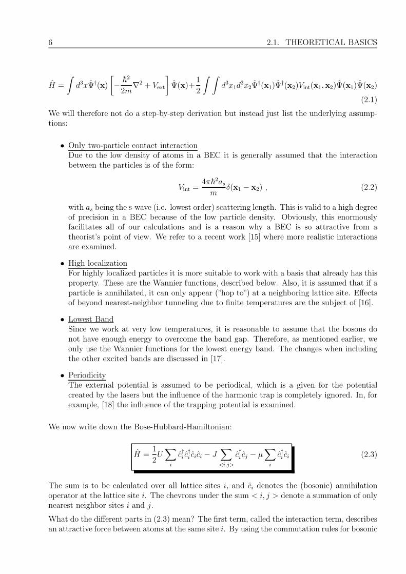
A thorough numerical calculation of U and V by using Wannier functions can be found in [20]. Itturns out that that U depends polynomially on V0 and J depends exponentially on V0. Dividingeq. 2.3 by J, we see that the influence of the laser strength seems only to manifest itself viaU/J , which will stay true for our further calculations in this thesis. But, this is not necessarily
8 2.1. THEORETICAL BASICS
Figure 2.1: J/U over Vr taken from [20]
always the case, since through Feshbach resonances it is possible to change the s-wave scatteringlength as, thereby influencing the particle interaction.
Vr stands for the laser potential V0 in units of the recoil energy ER = ~2π2
2a2m, with a being the
lattice spacing. Changing as would lead to a scaling of the y-axis with the factor a/as.
As mentioned, the two obvious choices for the starting point of further calculations are thestrong-coupling case where the hopping-term is introduced as a perturbation and the superfluidphase in which the interaction is small.
2.1.2 Phase transitions
A very broad and fascinating area of physics is concerned with phase transitions. A well-knowneveryday example is the evaporation or the solidification of liquid water: depending on externalvariables, such as pressure and temperature, the system can assume different states, or phases,in this case liquid, gaseous and solid. This diploma thesis will examine the phase transitionfrom the superfluid state to the Mott-insulator state of a BEC in an optical lattice, dependingon the externally adjustable laser strength. Common to all phase transitions is a discontinuityin a derivative of the appropriate thermodynamic potential, which were therefore classifiedaccording to when the first discontinuity appears (Ehrenfest classification). This has proven tobe too restrictive since there are examples for logarithmic and exponential singularities. Today,one usually only differentiates between first-order phase transitions where at least one partialderivative of a thermodynamic potential are discontinous, and second-order (or continous) phasetransitions.
The order parameter of a theory is a variable (in our case a scalar) defined such that it iszero for one phase and nonzero in the other. For a BEC, the order parameter is the particledensity for the ground state, n0 (actually, it is its squareroot). Another prominent example isthe energy gap ∆ in superconductors.
Some assumptions have to be made as to how the order parameter appears in the thermody-
CHAPTER 2. BEC IN OPTICAL LATTICES 9
namic potential. Some that have had much success are the Landau theory and the Φ4-theory.A very thorough treatment of the latter topic can be found in [21].
Within the Landau theory, the grand-canonical potential Ω is expanded with respect to theorder parameter Ψ up to fourth order. For symmetry reasons, only even powers appear.
Ω = aΨ4 + bΨ2 + c (2.6)
We can calculate the order parameter by demanding that Ω has a minimum:
∂Ω
∂Ψ= 4aΨ3 + 2bΨ = 0 (2.7)
and∂2Ω
∂Ψ2= 12aΨ2 + 2b > 0 (2.8)
In our coming calculations we will also derive the grand-canonical potential, but with respectto n0 which is actually Ψ2. Of course, this will also give us the minimum of Ω:
∂Ω
∂Ψ2=
∂Ω
∂Ψ
∂Ψ
∂Ψ2=
∂Ω
∂Ψ
1
2Ψ(2.9)
And, for Ψ 6= 0, both derivatives have the same set of solutions.
In this thesis, we will not analyze the regular phase transition to a BEC, but the phase transitionof a BEC in an optical lattice.Experimentally, the phase transition in an optical lattice was firstobserved in 2002 [22]. This Mott-superfluid-transition is called a quantum phase transition, thedifference to the general phase transition being that it also takes place at zero temperature dueto quantum fluctuations.
The change to the superfluid state in He4 is obviously also a phase transition. One might askwhether this is not another example of a Bose-Einstein condensate. Calculating TC , we get3.14K, close enough to the experimental value Tλ = 2.18K for the so-called lambda-point wheresuperfluidity sets in. We now know that the reasonable assumption of a BEC was not entirelycorrect. The fraction of the condensate at 0K is only about 1/12th, owing to the very stronginteractions in Helium. Furthermore, in 1972 He3 could be cooled down enough to about 2millikelvin to exhibit a superfluid state (this feat was awarded the Nobel Prize in Physics in1996 to David Lee, Robert Richardson and Douglas Osheroff). Since He3 consists of fermions,this cannot be a pure Bose Einstein condensate, for only through the strong correlations betweenthe atoms they are able to form pairs, which then are bosons able to condensate in the groundstate. Much research has been done concerning the BCS-BEC crossover, which is achieved bythe use of Feshbach resonances [23].
2.2 Experimental realization
In this chapter we give an overview of the experimental methods used to create a Bose-Einstein-Condensate and the difficulties that had to be overcome. Since this thesis will emphasizetheoretical calculations, just a rough overview will be provided. The methods used have becomeeven more refined during these last years, and we cannot explore all the details here.
10 2.2. EXPERIMENTAL REALIZATION
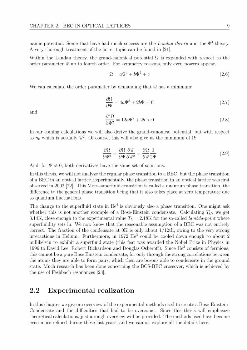
Figure 2.2: Phase diagram for T= 0 [24]. Only for integer density n there is a Mott insulator(MI) phase, a small deviation ǫ means the system always has a small part of particles thatcan move freely, a sign for the superfluid state (SF). The dashed line shows how changingthe chemical potential (which is in general space-dependent) means passing through severaldifferent phases.
CHAPTER 2. BEC IN OPTICAL LATTICES 11
As we already mentioned, the theoretical prediction of the occurrence of BEC took place manydecades before it could finally be experimentally realized. The main obstacle was to achievetemperatures low enough to allow for a macroscopic population of the ground state, though atthe same time not allowing the atoms to solidify in the process. At the start of every BEC, agas has to be produced by heating the atoms which gain enough thermic energy that they canleave the solid. Obviously, they then have a very high kinetic energy, which in the followingsteps must be reduced in order to observe a BEC.
The basic principle here is that of Doppler cooling, so named because it exploits the Doppler-shift of relative motion: due to the high velocity of the still hot particles, the frequency neededfor a transition between states is red-shifted. This can be used so that only particles around acertain velocity absorb a photon from an external laser. After a very short time, the particletransitions back to its former state by emitting again a photon. The difference is that duringthe absorbtion the particle receives momentum from the photon which leads to a decelerationwhile the emission spreads over all angels, i.e. no net momentum change occurs. More on LaserCooling can, for example, be found in [25]. For sodium, for example, a temperature as low as240µK can be reached by the Doppler mechanism alone.
Additionally, in a magneto-optical trap (MOT) an inhomogeneous magnetic field is superim-posed over the laser field for optical cooling. Due to the Zeeman-shift, the energy levels of theparticles change depending on their distance from the center of the trap in such a way that thechance for absorbing a photon increases with the distance, resulting in a net force towards thecenter, thereby trapping the particles.
The last and deciding step in creating a BEC is the evaporative cooling [26]. The basic ideais that, as temperature is a measure for the mean energy per particle, the temperature mustdecrease if the particles with the highest energy are removed.
The condition for an induced transition is:
gµBB = ~ω , (2.10)
with g the g-factor, µB the Bohr magneton and and ω the frequency of the field. The potentialseen by a particle in a magnetic field is
V = mF gµBB (2.11)
so by adjusting the spin state it is possible to change a particle from a low field seeking one to ahigh field seeking one, which results in the particle leaving the trap. By lowering the magneticfield, more particles will leave so trap so one can adjust the desired temperature (but acceptingthat always particles are lost) until BEC can be achieved. This typically takes only severalseconds.
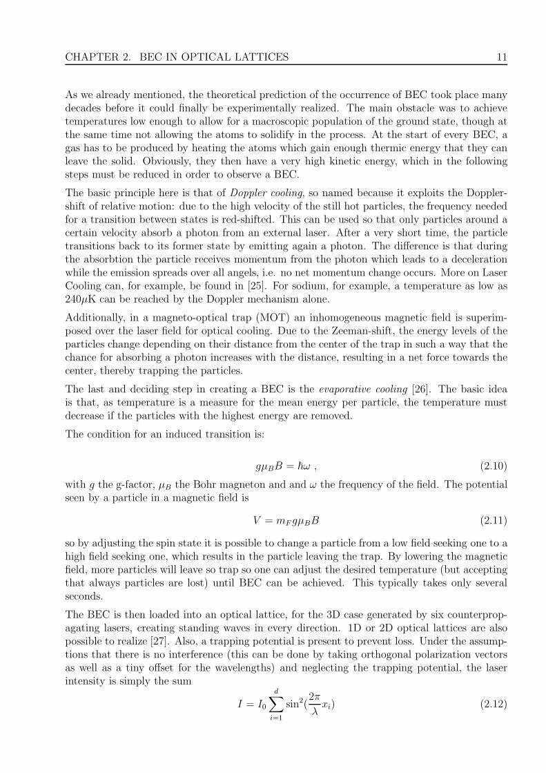
The BEC is then loaded into an optical lattice, for the 3D case generated by six counterprop-agating lasers, creating standing waves in every direction. 1D or 2D optical lattices are alsopossible to realize [27]. Also, a trapping potential is present to prevent loss. Under the assump-tions that there is no interference (this can be done by taking orthogonal polarization vectorsas well as a tiny offset for the wavelengths) and neglecting the trapping potential, the laserintensity is simply the sum
I = I0
d∑
i=1
sin2(2π
λxi) (2.12)
12 2.2. EXPERIMENTAL REALIZATION
Figure 2.3: Particles in the potential of an optical lattice [28].
(with λ being the laser wavelength) .
Perturbation theory for an external electric field acting as the perturbation (Stark effect) showsthat there is a linear correlation between I and the potential. With these assumptions, thepotential for the optical lattice reads:
V = V0
d∑
i=1
sin2(2π
λxi) (2.13)
We still haven’t answered the question how the existence of a BEC can actually be seen. Apartfrom indirect features like the existence of a gap in the MI state, there is a visually appealing wayby creating time-of-flight (TOF) pictures. This means that the trap is switched off completelyand the particles expand freely. Neglecting gravity, the time ∆t a particle needs to cover thedistance ∆r is related to the wave vector k simply as:
~k = p = mv = m∆r
∆t(2.14)
By measuring the distance and the time, one can therefore observe how many particles are ineach k-state. For T < TC one should begin to see a peak for k = 0 which gets more and morepronounced as the temperature is lowered.

CHAPTER 2. BEC IN OPTICAL LATTICES 13
Figure 2.4: TOF picture of the formation of a BEC at the MPQ.

14 2.2. EXPERIMENTAL REALIZATION
Chapter 3
Effective Hamiltonian for theBogoliubov Approximation
”More is different.”
Aphorism by P.W. Anderson
In this chapter we will study the Bogoliubov approximation [29] [30] , which is a suitable ansatzfor the case that the optical lattice depth is sufficiently low, so that we can assume that theBEC is essentially described by a macroscopic wave function plus a (small) correction term..
3.1 Bogoliubov Approximation
We call NS the number of lattice sites in the optical lattice we are studying, and write c†i forthe creation operator which creates one particle at the lattice site with the coordinates ri.
Statistical calculations with bosons at very low temperatures necessitate a special treatment ofthe ground state k = 0, which is macroscopically populated in the experiments we discuss here.It is therefore suitable to Fourier-transform the creation and annihilation operators:
ci =1√Ns
∑
k
ake−ik·ri , (3.1)
c†i =1√Ns
∑
k
a†keik·ri . (3.2)
The inverse relations are
ak =1√Ns
∑
i
cieik·ri , (3.3)
a†k =1√Ns
∑
i
c†ie−ik·ri . (3.4)
Note that the definitions are normalized in such a way that∑
i c†i ci =
∑k a
†kak, which means
that the sum of all particle number operators taken over all sites ri equals the sum of all particlenumber operators taken over all possible values for k. This sum obviously yields the value N ,
15
16 3.1. BOGOLIUBOV APPROXIMATION
the number of all particles, when applied to any state. In our calculations we shall make use ofthe following representation of the Dirac Delta-function:
∑
i
ei(k−k′)·ri = NSδk,k′ . (3.5)
With that, we can prove the above statement:
∑
i
c†i ci =∑
i
1
NS
∑
k
a†keik·ri
∑
k′
ak′e−ik′·ri =1
NS
∑
k
a†k∑
k′
ak′
(NSδk,k′
)=∑
k
a†kak . (3.6)
The Fourier components are operators which satisfy the ordinary commutation relations:
[ak, ak′ ] = [a†k, a†k′ ] = 0 , (3.7)
and [ak, a
†k′
]= δk,k′ . (3.8)
Eq. (3.7) is easy to prove, because ak and ak′ consist of sums of ci’s, which commute pairwisedue to the standard commutation relation [ci, cj] = 0. Likewise, all c†i ’s commute because
[c†i , c†j] = 0. The last missing commutation relation describes a mixed pair of creation and
annihilation operators:
[ak, a
†k′
]=
1
NS
[∑
i
cieik·ri ,
∑
j
c†je−ik′·rj
]=
1
NS
δi,j∑
i,j
e−(k·ri−k′·rj)[ci, c
†j
]=[ci, c
†i
]δk,k′ = δk,k′ .
(3.9)
Plugging (3.1) and (3.2) in the Bose-Hubbard Hamiltonian (2.3) thus yields:
H =1
2U
1
N2S
∑
i
∑
k
∑
k′
∑
k′′
∑
k′′′
a†ka†k′ ak′′ ak′′′eiri·(k+k′−k′′−k′′′)
− J1
NS
∑
<i,j>
∑
k
∑
k′
a†kak′eik·ri−k′·rj − µ1
NS
∑
i
∑
k
∑
k′
a†kak′eik·ri−k′·ri . (3.10)
This expression can be simplified as follows: We discuss here only the case of a cubic latticewith the lattice constant a, so that in the sum over next neighbors the sum over j just becomesrj = ri ± aep with p as a unit vector denoting the direction the neighbored lattice site lies.Therefore the Hamiltonian can be written as:
H =1
2U
1
N2S
∑
k
∑
k′
∑
k′′
∑
k′′′
a†ka†k′ ak′′ ak′′′
∑
i
eri·(k+k′−k′′−k′′′)
− J1
NS
∑
i
∑
k
∑
k′
eiri·(k−k′)∑
p=±1,2,...d
eiak′·ep − µ
1
NS
∑
i
∑
k
∑
k′
a†kak′eiri·(k−k′) . (3.11)
CHAPTER 3. EFFECTIVE HAMILTONIAN FOR THE BOGOLIUBOVAPPROXIMATION 17
By using the Euler-relation and the formula for the Delta-function (3.5), this gives:
H =1
2
U
NS
∑
k
∑
k′
∑
k′′
∑
k′′′
a†ka†k′ ak′′ ak′′′δ(k+k′),(k′′+k′′′) −
∑
k
[µ+
d∑
p=1
2J cos(kpa)
]a†kak . (3.12)
In the following, the starting point for our calculations will be the superfluid phase, so thatalmost all atoms in the trap occupy the ground state. If the laser strength is increased, oneobserves a behavior typical of a second order phase transition, and the corresponding orderparameter can be shown to be
√N0. We will see that this is approximately equal to the
expectation values of the creation and the annihilation operator for the ground state, < a0 > and< a†0 >, respectively: Indeed, since it follows from the definition of the expectation functionalapplied to an operator A in the grand-canonical ensemble,
< A >=tr(e−β(H−µN)A
)
tr(e−β(H−µN)
) 1 , (3.13)
that it is linear (the trace operator tr<.> is linear!), we have < a†0a0 >=< n0 >= N0
and < a0a†0 >=< a†0a0 + [a0, a
†0] >=< a†0a0 − 1 >= N0 − 1 ≈ N0, since in the superfluid phase
N0 ≫ 1.
Furthermore, the expectation value of the hermitian conjugated operator is just the complexconjugate of the operator’s expectation value:< O† >=< O >∗, so that we obtain < a0 >=< a†0 >=
√N0. In the deep superfluid regime,
we may thus assume that it is justified to write a0 =√N0 + δa0 and likewise for the creation
operator, in both cases the deviation from the mean value√N0 is supposed to be small, so that
we can neglect higher orders.
In the next step, we sort the terms by their order in the fluctuations δa0 and δa†0. The zerothorder terms are called Gross-Pitaevskii contributions, the first order terms vanish as we willsoon see, the second order ones are called Bogoliubov terms and the higher orders are neglectedfor now. As the title of this thesis suggests, we will later also need the higher order terms, sowe here list all orders.
We introduce here the dispersion relation
ǫk = 2Jd∑
p=1
1− cos(kpa) . (3.14)
This choice of the sign for the dispersion relation is chosen so that in the limiting case a → 0 weactually get the free dispersion ǫk ∝ k2: Taylor expansion at a = 0 up to second order yields:ǫk ∝
∑dp=1 1− (1−kp
2)+O(a3) ∝ k2, which is the expected quadratic dispersion. Furthermore,we have ǫ0 = 0, so that the energy scale starts at zero and never gets negative.
With the abbreviation z = 2d, z being the number of nearest neighbors, we can also writeǫk = Jz − 2J
∑dp=1 cos(kpa).
1The term −µN is already included in our Hamiltonian (2.3), so this term will not appear again in thefollowing calculations.

18 3.1. BOGOLIUBOV APPROXIMATION
We sort the orders by writing∑
kak = a0 +
∑k 6=0 ak.
0th order:All sums are replaced by
√N0 so only one term remains in this order:
H0int =
1
2UNSN
20 +N0(−Jz − µ) =
1
2Un0N0 +N0(−Jz − µ) (3.15)
1st order:Only one sum (= one fluctuation about N0) remains. There is no contribution from the quarticsum since in the δk+k′,k′′+k′′′ we have one k 6= 0 and all others are zero, so all terms in firstorder vanish. So we only have
−∑
k
[µ+
d∑
p=1
2J cos(kpa)
]a†kak (3.16)
2nd order:
H(2)int =
1
2Un0
∑
k
a†k∑
k′
a†k′ +
∑
k
a†k∑
k′′
ak′′ +∑
k′
a†k′
∑
k′′
ak′′
+∑
k
a†k∑
k′′′
ak′′′ +∑
k′
a†k′
∑
k′′′
ak′′′ +∑
k′′
ak′′
∑
k′′′
ak′′′
δk+k′,k′′+k′′′ +
∑
k
(ǫk − µ)aka†k
(3.17)
3rd and 4th order:
H(3)int =
1
2
U
NS
√N0
∑
k
a†k∑
k′
a†k′
∑
k′′
ak′′ +∑
k
a†k∑
k′
a†k′
∑
k′′′
ak′′′
+∑
k
a†k∑
k′′
ak′′
∑
k′′′
ak′′′ +∑
k′
a†k′
∑
k′′
ak′′
∑
k′′′
ak′′′
δk+k′,k′′+k′′′ .
(3.18)
The first two and the last two terms are equal after renaming the summation indices, since thischange also does not affect the δ.
H(4)int =
1
2
U
NS
δk+k′,k′′+k′′′
∑
k
ak†∑
k′
ak′†∑
k′′
ˆak′′
∑
k′′′
ˆak′′′ (3.19)
As mentioned, our effective Hamiltonian will only include terms up to second order in thefluctuations about
√N0, the higher orders will only play a role in later chapters, where we will
perform a perturbation expansion.
We can simplify H(2): renaming indices, the second and third as well as the fourth and fifthterm are equal
Heff = N0
(1
2Un0 − µ− zJ
)+ η
[∑′
k
a†kak(ǫk − Jz − µ+ 2Un0) +1
2Un0
∑′
k
aka-k + a†-ka†k
]
(3.20)
CHAPTER 3. EFFECTIVE HAMILTONIAN FOR THE BOGOLIUBOVAPPROXIMATION 19
Here η represents an artificial smallness to keep track of the order of the fluctuations. As soonas we need quantitative results, we will set η = 1.
The aim of the Bogoliubov transformation is to achieve a diagonal Hamiltonian in new creation
and annihilation operators bk and bk†, which depend linearly on the old ones. To this end we
make the following ansatz:
bk = uk · ak + vk · a†−k ,
b†−k = v∗k · ak + u∗k · a†−k . (3.21)
By taking the hermitian conjugate of the first equation and replacing k with -k we see bycomparing to the second equation that the coefficients uk and vk must not depend on the signof k:
uk = u−k ,
vk = v−k . (3.22)
Since we have shown in Eqs. (3.7) and (3.8) that ak and a†k obey the standard commutationlaws for creation and annihilation operators, we obtain
[bk, b†k′] = [ukak + vka
†−k, v
∗k′ ak′ + u∗
k′ a†−k′ ] = uku
∗k′ [ak, a
†−k′] + vkv
∗k′[a
†−k, ak′ ]
= uku∗k′δk,k′ − vkv
∗k′δk,k′ = (|uk|2 − |vk|2)δk,k′ ,
(3.23)
and see that, in order to retain the standard commutator relations, it is necessary that
|uk|2 − |vk|2 = 1 . (3.24)
This is also sufficient, since the remaining commutation relations are automatically fulfilled:
[bk, bk′ ] = [u(k)ak+v(k)a†−k, u(k′)ak′+v(k′)a†
−k′] = [ukak, vk′a†−k′]+[vka
†−k, uk′ak′ ] = 0 , (3.25)
since in our sums the case k = 0 is excluded, so that always k 6= −k .
Correspondingly, we obtain
[b†k, b†k′ ] = [v∗k′ ak + u∗
ka†-k, v
∗k′ ak′ + u∗
k′ a†-k′ ] = [v∗k′ ak, u
∗k′ a
†-k′] + [u∗
ka†-k, v
∗k′ ak′ ] = 0 (3.26)
with the same reasoning as above.
We now impose further conditions for the coefficients uk and vk by requiring that the Hamil-tonian (3.20) takes on a diagonal form like
Heff = α +∑′
k
(~ωk + β) +∑′
k
~ωkb†kbk . (3.27)

20 3.1. BOGOLIUBOV APPROXIMATION
In the following steps, we will frequently use that the identity∑
kf(k) =
∑kf(-k) is valid for
any function f and, since our sums exclude k = 0, we see from Eq. (3.8) that we can write:a−ka
†k = a†ka−k.
Our effective Hamiltonian (3.20) thus has the alternative representation
Heff = N0(1
2Un0 − µ− zt) +
1
2η
[∑′
k
(ǫk − Jz − µ+ 2Un0)+
∑′
k
Un0aka-k + Un0a†-ka
†k + (ǫk − Jz − µ+ 2Un0)a
†kak + (ǫk − Jz − µ+ 2Un0)a-ka
†-k
].
(3.28)
Now we use the inverse relations to (3.21),
ak = u∗kbk − vkb
†-k
a†−k = −v∗kbk + ukb†-k , (3.29)
and insert them in (3.44). Sorting by the different products of the new creation and annihilationoperators, we obtain:
b†kbk :1
2
[(ǫk − Jz − µ+ 2Un0) |uk|2 − Un0v
∗kuk − Un0u
∗kvk + ǫk − Jz − µ+ 2Un0) |vk|2
],
(3.30)
b-kb†-k :
1
2
[(ǫk − Jz − µ+ 2Un0) |uk|2 − Un0v
∗kuk − Un0u
∗kvk + (ǫk − Jz − µ+ 2Un0) |vk|2
],
(3.31)
b†kb†k : − 1
2
[2(ǫk − Jz − µ+ 2Un0)ukvk − Un0v
2k − Un0u
2k
], (3.32)
b-kbk : − 1
2
[2(ǫk − Jz − µ+ 2Un0)u
∗kv
∗k − Un0v
∗2k − Un0u
∗2k
]. (3.33)
We see that the last two equations are just complex conjugated to each other, if we remember(3.1) and (3.22), but this is not quite true for (3.30) and (3.31), as we have to commute bk andb†k. Since we demand that the bk‘s only appear in terms of the form ~ωkb
†kbk, we have reduced
the number of equations to two, and additionally still the condition (3.24) :
−1
2
[2(ǫk − Jz − µ+ 2Un0)ukvk − Un0v
2k − Un0u
2k
]= 0 . (3.34)
1
2
[(ǫk − Jz − µ+ 2Un0) |uk|2 − Un0v
∗kuk − Un0u
∗kvk + ǫk − Jz − µ+ 2Un0) |vk|2
]= ~ωk .
(3.35)
Since we have more variables than equations, we cannot expect a unique solution, however,that is not necessary at this point. First of all, we remark that a global phase factor cannotchange the Hamiltonian since it has U(1)-symmetry. Yet, we can answer the question how thephases of uk and vk are related relative to each other. This can be seen from Eq. 3.35, wherethe left-hand side must yield a real result. By writing uk = |uk| eiφuk and vk = |vk| eiφvk we

CHAPTER 3. EFFECTIVE HAMILTONIAN FOR THE BOGOLIUBOVAPPROXIMATION 21
see that after an arbitrary phase-shift the energy stays real iff φuk− φvk = 0 2 or, equivalently,
φuk= φvk . Later, we will proof that this also stays true for the second order terms. If we
assume at this point that the phase is arbitrary, the obvious choice is to make uk and vk real.
Now we can solve the above equations. First of all, u2k − v2k = 1 implies that we can write
uk = cosh x and vk = sinh(x). Equation 3.34 is of the form
2α(cosh x sinh x)− β(cosh2 x+ sinh2 x) = 0 . (3.36)
We rearrange this to
β
α= 2
cosh x sinh x
cosh2 x+ sinh2 x= 2
sinhxcoshx
1 + sinh2 xcosh2 x
= 2tanhx
1 + tanh2 x, (3.37)
which, by an addition theorem, is equal to tanh 2x. Using the following trigonometric identities,
cosh2 x =1
2(cosh 2x+ 1) =
1
2
(1√
1− tanh2 2x+ 1
)=
1
2
1√
1− β2
α2
+ 1
(3.38)
=1
2
(α√
α2 − β2+ 1
). (3.39)
we can now solve 3.35:
~ωk = α(cosh2 x+ sinh2 x)− 2β(sinh x cosh x) = α(α√
α2 − β2)− β2
α
α√α2 − β2
(3.40)
=α2 − β2
√α2 − β2
=√
α2 − β2, (3.41)
where we have used (3.36) to eliminate sinh x cosh x.
Writing out α and β yields:
|uk|2 = |vk|2 + 1 =1
2
(ǫk − Jz − µ+ 2Un0
~ω+ 1
)(3.42)
with the dispersion relation
~ωk =√
(ǫk − Jz − µ+ Un0)2 + 2Un0(ǫk − Jz − µ+ Un0) . (3.43)
At last, we now can write down our diagonal effective Hamiltonian. We must not forget toinclude 1
2~ωk, which arises due to the commutation performed in (3.31).
Heff = NS
(1
2Un2
0 − µn0 − Jzn0
)+
1
2
∑′
k
[~ωk − (ǫk − Jz − µ+ 2Un0)] +∑′
k
~ωkb†kbk
(3.44)
2The difference may also be a multiple of 2π, we neglect this ambiguity.
22 3.2. THE CONDENSATE DENSITY
3.2 The condensate density
We are ultimately interested in a relationship between the condensate density n0 and theexperimentally adjustable parameters U and J . Obviously, the number of all atoms mustequal the sum over the expectation values of all nk :
N = N0 +∑′
k
< a†kak > (3.45)
For calculating a trace we may use any basis, so in (3.45)we will choose one that is well-suited.Due to the fact that there are only one-particle contributions in our Hamiltonian (3.44), theoccupancy number representation |nα1 , nα2 · · · > yields such a basis, since their elements areeigenstates to H and to the new occupancy number operator b†kbk. The fact that all states used
for the trace are eigenstates to H simplifies the expectation value, since we can just apply Hin the denominator and the numerator and cancel the resulting eigenvalues. It just remains tocalculate tr(a†kak). To this end, we express the old creation and annihilation operators by thenew ones via (3.29) and get:
N = N0 + η
[∑′
k
< |uk|2 b†kbk + |vk|2 b−kb†−k − v∗ku
∗kb−kbk − vkukb
†kb
†−k >
]. (3.46)
The action of b†kbk = nk is obvious:
< nk1 , . . . |b†kbk|nk1 , · · · >=< nk1, . . . |nk|nk1 , · · · >= nk . (3.47)
Now, the first term in the sum is trivial, because the trace is a sum of its eigenstates. The secondterm likewise, if we commute the operators, which gives an additional factor |vk|2. The thirdand fourth term yield the expectation value zero, because they produce states with differentnk’s in the bra- and ket-vectors, which are orthogonal.
We introduce the particle density per site n:n = N
NS
n = n0 + η <
[1
NS
∑′
k
|uk|2 b†kbk + |vk|2 (b†kbk + 1)
]> . (3.48)
We insert (3.42) and remember that < b†kbk > is described by the Bose distribution. Now wehave our result,
n = n0 + η1
NS
[∑′
k
ǫk − Jz − µ+ 2Un0
~ωk
·(
1
eβ~ωk − 1+
1
2
)− 1
2
]. (3.49)
Since the experiments which we aim to explain are carried out at extreme low temperatures ofthe order of 10−8K, it is only natural to examine in particular the limit T → 0. This is easily
CHAPTER 3. EFFECTIVE HAMILTONIAN FOR THE BOGOLIUBOVAPPROXIMATION 23
done, since T → 0 means β → ∞ and therefore e−β~ω → 0. In the zero-temperature limit wethus have:
n = n0 + η1
NS
[∑′
k
1
2
(ǫk − Jz − µ+ 2Un0)
~ωk
− 1
2
]. (3.50)
For a numerical evaluation, we take the k’s to be sufficiently dense so that we may regard themas quasi-continuous. This allows us to change the sum to an integral via the general formula:
∑
k
f(k) 7−→∫
k
ρ(k)f(k)dk . (3.51)
Here ρ(k) denotes the density of states in k-space. Using periodic boundary conditions, the
states have a distance of 2πa
in every direction, so that one state occupies a volume of(2πa
)d,
which gives a density of ρ(k) =(
a2π
)d. Like in solid-state physics (the optical lattice has
obviously many similarities to the free electron model), we project all states in k-space ontothe first Brillouin zone
⊗di=1
(−π
a−→e i,
πa−→e i
).
Since we have originally just one state in a volume of the Brillouin zone, the density becomesmuch larger if we only take the integral from −π/a to +π/a, namely by the factor NS, thenumber of unit cells in k-space. We thus get:
n = n0 + η
1
NS
π/a∫
−π/a
NS
( a
2π
)d(1
2
(ǫk − Jz − µ+ 2Un0)
~ωk
− 1
2
)ddk
. (3.52)
For simplicity we introduce the dimensionless variable q := a2πk and get the following expression
that we will solve numerically:
n = n0 + η
12∫
− 12
12
(ǫ( 2π
aq) − Jz − µ+ 2Un0
)
~ω( 2πaq)
− 1
2
ddq . (3.53)
3.3 The grand-canonical potential and self-consistency
In this section we check whether our whole idea of diagonalizing and neglecting higher terms inthe Hamiltonian is consistent with the basic rules of thermodynamics. In particular, we verifythat we can also calculate the particle density n by differentiating the grand-canonical potentialwith respect to µ. The partition function Z is defined as tr(e−βH), where H is our effectiveHamiltonian (3.44). The so-called effective potential Veff is then calculated by − 1
βlnZ. This is
not yet the grand-canonical potential, since we still have a dependency upon n0, which is itselfa function of µ. This dependency must be eliminated. At first we get
Veff = − 1
βln tr
e
−βNS(12Un2
0−µn0−Jzn0)+η
[
12
∑′
k
(~ωk−(ǫk−Jz−µ+2Un0))+
∑′
k
~ωkb†kbk
] . (3.54)
24 3.3. THE GRAND-CANONICAL POTENTIAL AND SELF-CONSISTENCY
Like before, the appropriate basis for the calculation of the trace is the number occupancybasis. The terms without operators can simply be taken out of the trace, so for now we willlook only at the last sum:
− 1
βln tr
(e
∑′
k
−β~ωkb†kbk
)= − 1
βln
(∑
nk1
e−βnk1
)(∑
nk2
e−βnk2
)· · · = − 1
βln∏′
k
(∑
nki
e−βnki
)
= − 1
βln∏′
k
1
1− e−β~ωk
, (3.55)
where in the last step we have used the formula for the geometric series. By using the knownproperties of the logarithm can now write down the final result for the effective potential:
Veff = NS
(1
2Un2
0 − µn0 − Jzn0
)(3.56)
+ η
[1
2
∑′
k
(~ωk − (ǫk − Jz − µ+ 2Un0)) +1
β
∑′
k
ln(1− e−β~ωk
)]
. (3.57)
As said before, Veff is not a thermodynamic potential, yet it will become the grand-canonicalpotential Ω at the extremum with respect to n0: Solving ∂Veff
∂n0= 0 yields n0extr and Veff(n0 =
n0extr , µ, T, V ) is Ω(µ, T, V ) . This we will calculate in the next step.
∂Veff
∂n0= NS(−Jz − µ+ Un0) (3.58)
+ η
[1
2
∑′
k
(−2U +
∂~ωk
∂n0
)+
1
β
∑′
k
1
1− e−β~ωk
(−e−β~ωk
)(−β)
∂~ωk
∂n0
](3.59)
By looking at (3.43), we can calculate that
∂~ωk
∂n0=
U(2ǫk − 2Jz − 2µ+ 3Un0)
~ωk
, (3.60)
which we plug in and get:
0 = NS(−Jz − µ+ Un0) + η
U∑′
k
[(2ǫk − 2Jz − 2µ+ 3Un0)
~ωk
(1
2+
1
eβ~ωk − 1
)− 1
].
(3.61)
One important result from this equation is that, in the lowest order in η, we can write
n0 =Jz + µ
U+O(η) . (3.62)
We now re-insert this result in (3.61), and since we disregard orders of η higher than one, wecan just insert the lowest order for n0 in those terms that already are of first order in η.

CHAPTER 3. EFFECTIVE HAMILTONIAN FOR THE BOGOLIUBOVAPPROXIMATION 25
n0 =Jz + µ
U− η
[1
NS
∑′
k
(2ǫk + Jz + µ)
~ωk
(1
2+
1
eβ~ωk − 1
)− 1
]+O(η2) . (3.63)
This result must be inserted in Eq.(3.57) in order to obtain the grand-canonical potential Ω upto first order in η:
Ω = −NS
2U(Jz + µ)2 +
η
2
∑′
k
(~ω
(0)k − ǫk − Jz − µ
)+
1
β
∑′
k
ln(1− e−β~ω
(0)k
]. (3.64)
Here and in the following, we will often omit the O(η2), because we do not need to emphasizeevery time that we neglect higher orders in η. Inserting (??) in (3.43) results in the zerothorder of ~ωk.
~ωk(0) =
√(ǫk + µ− µ)2 + 2
[(Jz + µ)2 − (zJ + µ) (−ǫk − Jz + µ)
]
=√
ǫ2k + 2ǫk (Jz + µ) . (3.65)
For checking the self-consistency we now need the particle density n which we get with the helpof the grand-canonical potential: n = − 1
NS
∂Ω∂µ.
With very similar calculations as before, we get:
∂~ω(0)k
∂µ=
ǫk
~ω(0)k
, (3.66)
and therefore:
n =(Jz + µ)
U+
1
NSη
[∑′
k
(−ǫk)
~ω(0)k
(1
2+
1
eβ~ω(0)k − 1
)+
1
2
]. (3.67)
To see the equivalence to (3.49), we insert the equation (3.63) for n0 and subtract:
n− n0 =(Jz + µ)
U− (Jz + µ)
U+ η
1
NS
[∑′
k
−ǫk + Jz + 2ǫk + µ
~ω(0)k
(1
2+
1
eβ~ω(0)k − 1
)− 1 +
1
2
]
(3.68)
= η1
NS
[∑′
k
1
~ω(0)k
(1
2+
1
eβ~ω(0)k − 1
)(ǫk + Jz + µ)− 1
2
](3.69)
We are almost done, we just remember that according to (3.62) we have in zeroth order2 (Jz + µ) = 2Un0, so that
n− n0 = η1
NS
[∑′
k
1
~ω(0)k
(1
2+
1
eβ~ω(0)k − 1
)(ǫk − Jz − µ+ 2Un0)−
1
2
]. (3.70)

26 3.4. PLOTS FOR T = 0
We see that we have indeed gotten the same result as in (3.49) in two different ways, which showsthe inner consistency of the Bogoliubov approximation. We can now eliminate the chemicalpotential µ, which we achieve by substituting Eq. (??) in (??), which yields
n− n0 = η1
NS
[∑′
k
1
~ωk
(1
2+
1
eβ~ωk − 1
)(ǫk + Un0)−
1
2
], (3.71)
and we likewise get for the integral in (3.53):
n = n0 + η
12∫
− 12
[1
2
(ǫ( 2πaq) + Un0)
~ω( 2πaq)
− 1
2
]ddq , (3.72)
a result also obtained in [29].
We now check whether our result (3.71) gives the correct results in the limit UJ
→ 0, whichshould of course result in the model for free Bosons. At first we take the temperature to be
zero, so we consider n − n0 = η[∑′
k
1~ωk
12(−ǫk + 2Jz + Un0)− 1
2
]. Now we only examine
the expression in the sum. We can easily perform the limit:
U
Jn0 +
ǫkJ
UJ→0−→ ǫk
J√(U
Jn0 +
ǫkJ
)2
+ 2U
Jn0
(U
Jn0 +
ǫkJ
)UJ→0−→√(ǫk+Jz
J
)2(3.73)
We now insert the definition (3.14) of ǫk and thus get
2∑d
p=1 (1− cos(kpa))∣∣∣2∑d
p=1 (1− cos(kpa))∣∣∣. (3.74)
Since |cos| ≤ 1, the enumerator is positive, so the fraction just gives the value +1. We alsosee that in the sum we have the values +1
2and −1
2which cancel each other out, therefore the
result, as expected for Bosons at zero temperature, states that n = n0, i.e. all Bosons occupythe ground state.
Next, we examine the case of a finite temperature. We encounter the same fraction as before,which again gives the value +1, and so the result is
n = n0 + η∑′
k
1
eβ~ωk − 1, (3.75)
which is just the Bose-Einstein distribution, so again the correct limit is obtained.
3.4 Plots for T = 0
After having shown the inner consistency of our ansatz, we now turn to a plot of Eq. (3.53).In order to do that, we have to have µ eliminated, which we already did in Eq. (3.72), which
CHAPTER 3. EFFECTIVE HAMILTONIAN FOR THE BOGOLIUBOVAPPROXIMATION 27
0 500 1000 1500 2000
0.0
0.2
0.4
0.6
0.8
1.0
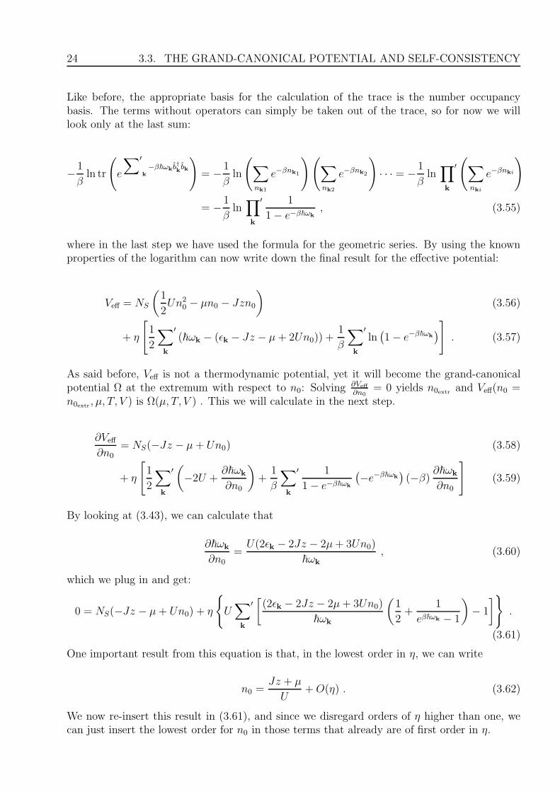
Figure 3.1: The condensate density n0 relative to n versus UJin d = 3 dimensions. The solid
line represents n=1, the dashed line stands for n = 0.5 .
we plot by numerical calculations. The Bogoliubov approach will be a good model in the deepsuperfluid regime, since there most of the atoms populate the ground state. That in turnmeans we do not make great errors when neglecting higher orders of η, which was introducedas the deviation from the case that all atoms assume the state k = 0. In the figure we plotthe condensate fraction n0
nversus U
J. We expect that for U
J= 0, all atoms occupy the ground
state, so the condensate fraction should be equal to one. For higher values of UJ, the condensate
fraction decreases monotonically, until it (hopefully) reaches zero at a value we will call UJ crit
.Monte-Carlo calculations [31] which have been shown to agree very well with the experimentalresults [32] predict the critical value to be at about 29.
In Fig. (3.1) we plot the three-dimensional case with two different values for n. The plots showthat our theory unfortunately does not predict the quantum phase transition we hoped for. Assaid before, the Bogoliubov approach will provide the best results in the deep superfluid phase,and the phase transition seems to be beyond its area of validity. Indeed, we can see that thismust be the case: the phase transition is defined by the value of U
Jwhere n0 = 0. Inserting
that yields ~ω = ǫk which means the whole integrand in 3.72 becomes zero and we get n = 0,therefore obviously no phase transition takes place within the simplifications of our model.
It is therefore necessary to modify our theory so that its scope reaches farther into the Mott-insulator regime.
3.5 Popov approximation
The Popov approximation is an application of variational perturbation theory to expand thearea of validity of the Bogoliubov approach in the hopes of finding a phase transition at highvalues of U/J . We follow an earlier work in our research group [33], who used the Path-Integralformalism but, stemming from an operator-ordering ambiguity in this formalism, did not getthe same result we did.
28 3.5. POPOV APPROXIMATION
To this end, we make a variational ansatz for µ by setting
µ = M + η∆ , (3.76)
and replacing µ in Ω with again neglecting terms of higher order in η than one. We will callthe result Ω. Again, in the terms that already are in first order of η, we just need to insert thezeroth order for µ.
Ω = −NS
2U
(J2z2 + 2JzM + 2Jzη∆+ 2Mη∆+M2
)
+ η∑′
k
[~ω
(0)k − ǫk − 2Jz −M
2+
1
βln(1− e−β~ω(0)
)]+O
(η2). (3.77)
Here ω(0) is just ω(0) with µ replaced by M . We get rid of any remaining dependency on ∆ byinserting the relation (3.76) again via ∆ = µ−M
η:
Ω = −NS
2U
(J2z2 −M2 + 2Jzµ + 2Mµ
)
+ η∑′
k
[~ω
(0)k − ǫk − 2Jz −M
2+
1
βln(1− e−β~ω(0)
)]+O
(η2). (3.78)
In order to eliminate the dependancy of ω(0)k on M we differentiate Ω with respect to M , set
the result equal to zero and insert the solution, which is Mextr:
0 =∂Ω
∂M=
NS
U(M − µ) + η
[∑′
k
(ǫk)
~ω(0)k
(1
2+
1
eβ~ω(0)k − 1
)− 1
2
]. (3.79)
Obviously, under the sum just the same terms as in Eq. (3.67) arise, because the operationsare the same with the replacement µ 7−→ M .
We solve Eq. (3.79) for Mextr, which gives:
Mextr = µ− U
NS
η
[∑′
k
(ǫk)
~ω(0)k
(1
2+
1
eβ~ω(0)k − 1
)− 1
2
]. (3.80)
In the next step, we calculate n (M) using N = nNS = −∂Ω∂µ. The chain rule and the fact that
Ω = Ω (M) |M=Mextr allows to rewrite this as:
nNS = −∂Ω
∂µ= −∂Ω (µ,Mextr (µ))
∂µ
∣∣∣∣∣M=Mextr
=
(−∂Ω
∂µ− ∂Ω
∂Mextr
∂Mextr
∂µ
)∣∣∣∣∣M=Mextr
. (3.81)
But from the definition in Eq. (3.79) we see that ∂Ω∂M
= 0, when M = Mextr, so
CHAPTER 3. EFFECTIVE HAMILTONIAN FOR THE BOGOLIUBOVAPPROXIMATION 29
0 20 40 60 80 100
0.0
0.2
0.4
0.6
0.8
1.0
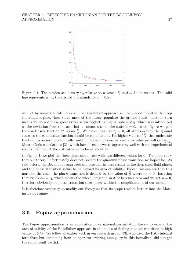
Figure 3.2: The condensate density n0 relative to n versus UJin the Popov-approximation for
n = 1.
nNS = −∂Ω
∂µ= −∂Ω
∂µ
∣∣∣∣∣M=Mextr
3.78=
NS
U(Jz +Mextr) . (3.82)
We now need also n0 (Mextr) in order to write down an improved Eq. (3.63). That means, wewill again use the variational ansatz (3.76), this time in Eq. (3.63), which yields:
n0 =Jz + µ
U− η
1
NS
∑′
k
[(2ǫk + Jz +M)
~ω(0)k
(1
2+
1
eβ~ω(0)k − 1
)− 1
], (3.83)
where in terms that already are of first order in η, we just needed to substitute µ 7−→ M . Nowwe use Eq. (3.80) to eliminate the chemical potential µ which yields:
n0 =Jz +M
U− η
1
NS
∑′
k
[(ǫk + Jz +M)
~ω(0)k
(1
2+
1
eβ~ω(0)k − 1
)− 1
2
]. (3.84)
Now, we want to eliminate the parameter M , which is done by inserting Eq.(3.82) for M :
n0 =Jz + (Un− Jz)
U− η
1
NS
∑′
k
[(ǫk + Jz + Un− Jz)
~ωk
(1
2+
1
eβ~ωk − 1
)− 1
2
]
= n− η1
NS
∑′
k
[(ǫk + Un)
~ωk
(1
2+
1
eβ~ωk − 1
)− 1
2
].
(3.85)
By comparing this result to (3.71), we see that the result of the Popov-approximation is almostidentical to the result we got before, except that we replaced n0 7−→ n in the sum, i.e. thecondensate density with the particle density.
This result could have been obtained much easier, since we could have seen from Eq.(3.49) thatn0 = n + O (η), which, when re-inserted would have yielded Eq.(3.85). We plot our newfoundresults, and see that the Popov approximation has indeed succeeded in introducing a quantum

30 3.5. POPOV APPROXIMATION
0 20 40 60 80 100 120 140
0.0
0.2
0.4
0.6
0.8
1.0
Figure 3.3: The condensate density n0 relative to n versus UJin the Popov-approximation for
n = 2.
0 50 100 150 200
0.0
0.2
0.4
0.6
0.8
1.0
Figure 3.4: The condensate density n0 relative to n versus UJin the Popov-approximation for
n = 3.

CHAPTER 3. EFFECTIVE HAMILTONIAN FOR THE BOGOLIUBOVAPPROXIMATION 31
phase transition. Looking back at fig. (2.2) we can also see the qualitatively correct behavior:for greater n, J/U crit becomes smaller, i.e. U/Jcrit becomes larger. Encouraged by this positiveresult, we now go to one order higher, in order to come closer to the expected value of 29 (asmentioned above) for n = 1.

32 3.5. POPOV APPROXIMATION
Chapter 4
Beyond the Bogoliubov approximation:second order
”If we are facing in the right direction, all we have to do is keep on walking.”
Buddhist Saying
As the title of this thesis suggests, we will not stop with the level of approximation we didthus far but want to investigate also how to include higher orders. The terms of third (3.18)and fourth (3.19) order in the fluctuations represent the perturbation V to our diagonalizedHamiltonian.
4.1 How perturbation theory for T 6= 0 works
Quantum theory in the operator formalism is usually expressed in one of three choices: theSchrodinger picture, in which the time evolution of the system manifests itself in the states,whereas the operators can only be explicitly time-dependent. The Heisenberg picture turnsthis around, here the states are time-invariant. For our purposes, we will use the Dirac (orinteraction) picture which already assumes that the Hamiltonian can be separated into a free,time-independent part H0 and a perturbation V : H = H0+ V . The time evolution of the statesis governed by V , whereas that of the operators depends only on H0 via AD(t) = e
i~H0tAe−
i~H0t,
where A denotes the operator in the Schrodinger picture. At t = 0 both pictures coincide. Howthis is accomplished in detail can be found in every standard textbook, e.g. [34]. As we hadseen in the introduction, all interesting properties of a macroscopic system can be calculated bythe respective thermodynamic potential. We now give a short derivation for the perturbationexpansion of the grand-canonical potential in imaginary time:
The perturbation manifests itself twice in Ω, in the perturbation series of the time-evolutionoperator U and in the factor e−βH . We will see that it is much simpler to introduce theWick-rotation τ = it. In the Dirac-picture, the time-evolution operator U obeys the followingequation of motion:
−~∂U (τ, τ ′)
∂τ= V (τ)U(τ, τ ′) (4.1)
with the initial condition U(τ, τ) = 1.
33
34 4.2. THE WICK THEOREM
Formal integration and n-times iteration of the result yields with setting τ ′ = 0:
U(τ, 0)(n) =
n∑
k=0
1
k!
(−1
~
)kτ∫
0
dτ1 . . . dτkT(V (τ1) . . . V (τk)
), (4.2)
where T is the time-ordering operator 1, which sorts the operators in its argument with de-creasing time from left to right.
From the explicit form of the Dirac time-evolution operator
U(τ, τ ′) = eH0~
τe−H0~
(τ−τ ′)e−H0~
τ ′ (4.3)
and setting τ ′ = 0,it can easily be seen that e−1~Hτ = e−
1~H0τ U(τ, 0) . By setting τ = ~β, we
get for the partition function:
Z = tr(e−βH
)= tr
(e−βH0U(~β, 0)
)(4.4)
=∞∑
n=0
1
n!
(−1
~
)nτ∫
0
dτ1 . . . dτntre−βH0 T(V (τ1) . . . V (τn)
) . (4.5)
This series conveniently sorts by the order in the perturbation V and is the starting point forfurther calculations in T > 0 perturbation theory.
4.2 The Wick theorem
In second quantization all operators are expressed by creation and annihilation operators. Theproblem to tackle now is thus how the time-ordered product of several annihilation and creationoperators in the Dirac-picture looks like. An invaluable help when evaluation the time-orderedproduct is the Wick-theorem ( [35], [36]). It states that the expectation value of a time-orderedproduct of creation and annihilation operators is equal to the expectation value of the time-ordered product of all possible pairs of creation and annihilation operators (one such pairis called a contraction). Usually, the Hamiltonian conserves the particle number, thereforeonly the pairs with one creation and one annihilation operator contribute. The expression−〈T (ak(τ)ak′(τ ′))〉 is called the free Green function Gk(τ, τ
′) and is a fundamental quantitythat will appear when we apply the Wick theorem. We remember that in the Dirac-picture thetime-dependence is of the form
O(τ) = e1~H0τ Oe−
1~H0τ . (4.6)
Using [bk, nk′ ] = [bk, b†k′ bk] = bk′[bk, b
†k′]+[bk, bk′]b†
k′ = δk,k′ bk+0 and, similarly [b†k, nk′] = δk,k′ b†k,
we can show that for an Hamiltonian of the form H0 =∑
k ~ωknk we have
bk(τ) = e−1~~ωkτ bk
1We remark that we use this definition since we will only work with bosons, for fermions the sign of thepermutation needed to yield the correct time ordering must be included.
CHAPTER 4. BEYOND THE BOGOLIUBOV APPROXIMATION: SECOND ORDER 35
andb†k(τ) = e
1~~ωkτ b†k , (4.7)
so the time-dependence appears in such a way that the usual commutation rules are kept i.e.we can still speak of these operators as construction and annihilation operators.
Proof : We show that
bk(∑
k′
~ωk′nk′)n = (~ωk +∑
k′
~ωk′nk′)nbk (4.8)
for n ∈ N.
For n = 1, this follows from the remark above:
bk∑
k′
~ωk′ nk′ = [bk,∑
k′
~ωk′ nk′] +∑
k′
~ωk′nk′ bk = ~ωkbk +∑
k′
~ωk′nk′ bk (4.9)
The induction step follows similarly:
bk(∑
k′
~ωk′ nk′)n+1 = bk(∑
k′
~ωk′nk′)n∑
k′
~ωk′nk′ = (~ωk +∑
k′
~ωk′nk′)nbk∑
k′
~ωk′ (4.10)
= (~ωk +∑
k′
~ωk′ nk′)n+1
bk X (4.11)
We can use this to see
bk(τ) = eτ~
∑
k′ ~ωk′ bke− τ
~
∑
k′ ~ωk′ = eτ~
∑
k′ ~ωk′ bk
∞∑
n=0
1
n!
−τ
~
n
(∑
k′
~ωk′nk′)n (4.12)
= e−τ~
∑
k′ ~ωk′
∞∑
n=0
1
n!
[−τ
~(~ωk +
∑
k′
~ωk′ nk′)
]n= e−
τ~ωk bk , (4.13)
where we used in the last step that∑
k′ ~ωk′ nk′ commutes with c-numbers so we can use thate
τ~
∑
k′ ~ωk′e−τ~
∑
k′ ~ωk′ = 1.
(4.7) can be proven in a similar fashion, alternatively we remember that the property of twooperators being Hermitian is time-independent.
We will later need ak(τ) and ak(τ), so we calculate these too. Luckily, their time-dependenceis very similar:
ak(τ) = e1~H0τ ake
− 1~H0τ = e
1~H0τ(ukbk − vkb
†-k
)e−
1~H0τ = ukbk(τ)− vkb-k(τ) (4.14)
and
ak(τ)† = e
1~H0τ ake
− 1~H0τ = e
1~H0τ(ukbk − vkb
†-k
)e−
1~H0τ = ukbk(τ)− vkb-k(τ) . (4.15)
So, in a sense, including a time-dependence in the Dirac-picture and the Bogoliubov transfor-mation commute, which is very comforting since in the following we can conveniently choosewhich operation to perform first.
36 4.3. BEYOND BOGOLIUBOV
Next, we observe that the Green function depends only on the time-difference of its arguments,which is easily proven by using the trace’s cyclical commutativity:
Gk(τ′, τ ′′) = Gk(τ
′ − τ ′′) =: Gk(τ) (4.16)
An interesting complication arises in our calculations because of the Bogoliubov transformation.When calculating the trace in the free basis of the bk′s, the ak′s are not diagonal anymore. Wetherefore also have to calculate the a− a and the a† − a† correlations. At this point one mustask the question whether the ad-hoc prescription of the time-ordering operator acting just asthe unity operator at equal times stays valid when using the Bogoliubov transformation. Thisis indeed the case, which we will later show for H(4) as an example by explicitly calculating thecontractions in two possible ways.
4.3 Beyond Bogoliubov
Via the Bogoliubov transformation we succeeded in getting one diagonalized part of the Hamil-tonian, which we will denote H0, and the remaining terms of third and fourth order in thefluctuations around the ground state, H3 and H4, which play the role of a perturbation. Up tosecond order in this perturbation, we have:
Z(2) = tr
e−βH0
[1+
~β∫
0
(H3(τ)+H4(τ))dτ+
~β∫
0
~β∫
0
(H3(τ1) + H4(τ1)
)(H3(τ2) + H4(τ2)
)dτ1dτ2
]
(4.17)
From the standard examples we expect for all expectation values of terms with an unevennumber of creation and annihilation operators to vanish. This is also true in our case since an(un-)even number of a-operators implies an (un-)even number of b-operators. The expectationvalue is calculated in the basis of eigenstates to H(0), so all terms containing only one power ofH(3) are zero.
We now encounter a little problem with defining the order of the perturbation, since we ac-tually have combined two: first, the deviations from the condensate ground-state N0, whichwe included up to second order. The higher orders then were introduced as a perturbation V .
So, one could, for example, ask the question whether H(3)2 or H(4)2 should also belong to oursecond order.
In the Path-Integral formalism the answer is widely known: the order of the loop-expansion
corresponds to the order of ~ (cf. [37]). We will see that the 2-loop-term consists of H(4)
and
H(3)2.
4.4 The H(4) term
This term (cf. 3.19) is of the form
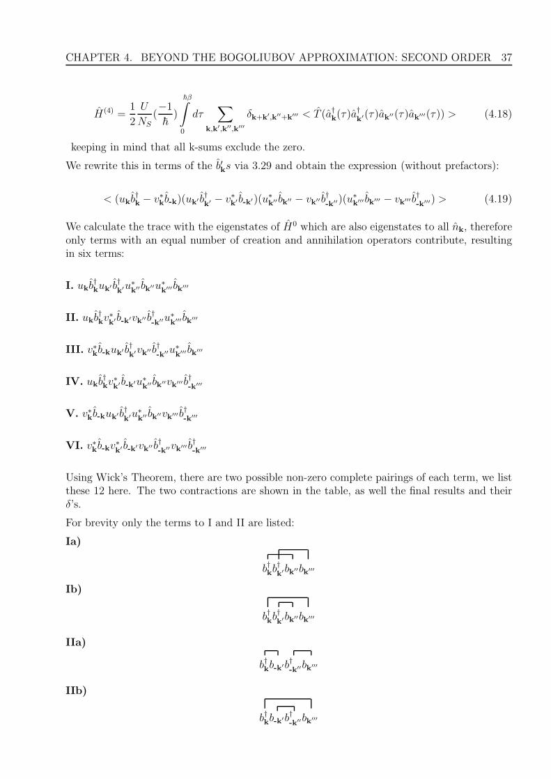
CHAPTER 4. BEYOND THE BOGOLIUBOV APPROXIMATION: SECOND ORDER 37
H(4) =1
2
U
NS(−1
~)
~β∫
0
dτ∑
k,k′,k′′,k′′′
δk+k′,k′′+k′′′ < T (a†k(τ)a†k′(τ)ak′′(τ)ak′′′(τ)) > (4.18)
keeping in mind that all k-sums exclude the zero.
We rewrite this in terms of the b′ks via 3.29 and obtain the expression (without prefactors):
< (ukb†k − v∗kb-k)(uk′ b†
k′ − v∗k′ b-k′)(u∗k′′ bk′′ − vk′′ b†
-k′′)(u∗k′′′ bk′′′ − vk′′′ b†
-k′′′) > (4.19)
We calculate the trace with the eigenstates of H0 which are also eigenstates to all nk, thereforeonly terms with an equal number of creation and annihilation operators contribute, resultingin six terms:
I. ukb†kuk′ b†
k′u∗k′′ bk′′u∗
k′′′ bk′′′
II. ukb†kv
∗k′ b-k′vk′′ b†
-k′′u∗k′′′ bk′′′
III. v∗kb-kuk′ b†k′vk′′ b†
-k′′u∗k′′′ bk′′′
IV. ukb†kv
∗k′ b-k′u∗
k′′ bk′′vk′′′ b†-k′′′
V. v∗kb-kuk′ b†k′u∗
k′′ bk′′vk′′′ b†-k′′′
VI. v∗kb-kv∗k′ b-k′vk′′ b†
-k′′vk′′′ b†-k′′′
Using Wick’s Theorem, there are two possible non-zero complete pairings of each term, we listthese 12 here. The two contractions are shown in the table, as well the final results and theirδ’s.
For brevity only the terms to I and II are listed:
Ia)
b†kb†k′bk′′bk′′′
Ib)
b†kb†k′bk′′bk′′′
IIa)
b†kb-k′b†-k′′bk′′′
IIb)
b†kb-k′b†-k′′bk′′′

38 4.4. THE H(4) TERM
I.aukuk′u∗
k′′u∗k′′′
b†kbk′′ b†kbk′′ δk,k′′δk′,k′′′ = |uk|2 |uk′|2 〈nk〉〈nk′〉I.b b†kbk′′′ b†
k′ bk′′ δk,k′′′δk′,k′′ = |uk|2 |uk′|2 〈nk〉〈nk′〉II.a
ukv∗k′vk′′u∗
k′′′
b†kb-k′ b†-k′′ bk′′′ δk,-k′δ-k′′,k′′′ = ukv
∗kvk′′u∗
k′′〈nk〉〈n−k′′〉II.b b†kbk′′′ b−k′ b†
−k′′ δk,k′′′δ−k′,-k′′ = |uk|2 |vk′ |2 〈nk〉〈n−k′+1〉III.a
v∗kuk′vk′′uk′′′
b−kb†k′ b†
−k′′ bk′′′ δ−k,k′δ−k′′,k′′′ = v∗k′uk′vk′′′u∗
k′′′〈n−k + 1〉〈nk′′′〉III.b b−kb
†−k′′ b†
k′ bk′′′ δ−k,−k′′δk′,k′′′ = |vk|2 |uk′ |2 〈n-k + 1〉〈nk′〉IV.a
ukv∗k′u∗
k′′vk′′′
b†kb−k′ bk′′ b†-k′′′ δk,−k′δk′′,−k′′′ = ukv
∗kvk′′u∗
k′′〈nk〉〈nk′′ + 1〉IV.b b†kbk′′ b−k′ b†
−k′′′ δk,k′′δ−k′,−k′′′ = |uk|2 |vk′ |2 〈nk〉〈n−k′ + 1〉V.a
v∗kuk′u∗k′′vk′′′
b−kb†k′ bk′′ b†
−k′′′ δ−k,k′δk′′,−k′′′ = ukv∗kvk′′u∗
k′′〈n−k + 1〉〈nk′′ + 1〉V.b b−kb
†−k′′′ b†
k′ bk′′ δ−k,−k′′′δk′,k′′ = |vk|2 |uk′ |2 〈n−k + 1〉〈nk′〉VI.a
v∗kv∗k′vk′′vk′′′
b−kb†−k′′ b−k′ b†
−k′′′ δ−k,−k′′δ−k′,−k′′′ = |vk|2 |vk′|2 〈n−k + 1〉〈n−k′ + 1〉VI.b b−kb
†−k′′′ b−k′ b†
−k′′ δ−k,−k′′′δ−k′,−k′′ = |vk|2 |vk′|2 〈n−k + 1〉〈n−k′ + 1〉
Table 4.1: Terms coming from H(4)
As we have seen, a contraction of construction operators at equal times just corresponds totheir expectation value. We get for the above examples:
Ia) |uk|2 |uk′|2 < nk >< nk′ > δk,k′′δk′,k′′′
Ib) |uk|2 |uk′ |2 < nk >< nk′ > δk,k′′′δk′,k′′
IIa)ukv∗kvk′′uk′′′ < nk >< nk′′ > δk,-k′δ-k′′,k′′′
IIb)|uk|2 |vk′ |2 < nk > (< nk′ > +1)δk,k′′′δk′,k′′
It is an important observation that the initial δk+k′,k′′+k′′′ just acts as the identity operator.That can be seen in 8 of the 12 terms (for example Ia, Ib, IIb) where two δ ’s arise from thecontractions which relate k′s from the same side in the initial δ. Take, for example Ia): wehave δk,k′′ and δk′,k′′′ so our initial δ takes the form δk+k′,k+k′ , which is trivially always equalto one. Therefore, we still have two summations. In IIa) as an example for the remaining fourterms, we have δk,-k′ and δ-k′′,k′′′ , which implies δk−k,k′′−k′′ , also always equal to one.
Now we think about how we can use some symmetries to reduce the number of terms we needto calculate. It is clear that
∑k bk =
∑k b-k. uk and vk are per definition symmetric. In the
same eight terms mentioned above the minus signs appear only pairwise on the δ′s (or not atall) and since δ-k,-k′ = δk,k′, in these terms we can replace -k by k.
When introducing the Bogoliubov transformation we saw that a number of prefactors u and vare valid solutions to our problem. We had assumed that the phases of uk and vk should beequal. A posteriori we can see from our result that this assumption was correct, since in the
CHAPTER 4. BEYOND THE BOGOLIUBOV APPROXIMATION: SECOND ORDER 39
H(3)-term the phase φ will cancel out also, as we will soon see.
By renaming the dummy integration variables we can reduce the number of different terms tosix. It is to be understood that we have two remaining k-sums, here named k and k′.
1)|uk|2 |uk′ |2 〈nk〉〈nk′〉 , (these are the terms Ia and Ib)
2)|vk|2 |vk′ |2 (〈nk〉+ 1)(〈nk′〉+ 1) (VIa and VI b)
3)|uk|2 |vk′|2 〈nk〉(〈nk′〉+ 1) (IIb, IIIb, IVb, Vb)
4)ukvkuk′vk′〈nk〉〈nk′〉 (once, this is IIa)5)ukvkuk′vk′(〈nk + 1)〉(〈nk′〉+ 1) (Va)
6)ukvkuk′vk′〈nk〉(〈nk′〉+ 1) (IIIa and IVa)
Now that we have gathered all arising terms, we can proceed to sum them up. The time-integral will be trivial, since from eq. (4.7) we see that the time-dependence is expressed by anexponential function, but with different signs for creation and annihilation operators. Since acontraction is always between these two, the time-dependence just cancels out and the integralsimply yields the prefactor ~β.
H(4) =1
2
U
NS
∑
k,k′
−1
~~β [ukvk (2〈nk〉+ 1)uk′vk′ (2〈nk′〉+ 1)]
+2[u2k〈nk〉+ v2k (〈nk〉+ 1)
] [u2k′〈nk′〉+ v2k′ (〈nk′〉+ 1)
](4.20)
We will soon see how these terms appear in a diagrammatical depiction.
4.5 The H(3)2-term
We had already calculated the form of H(3) in 3.18.
H(3) =√
N0U
NS
∑
k,k′,k′′,k′′′
a†ka†k′ ak′′δk+k′,k′′ + a†kak′ ak′′δk,k′+k′′ (4.21)
In the H(3)2-term we therefore get the sum of four different expressions, each consisting of sixoperators, three each at τ1 and three at τ2. For every expression, there are (6-1)!! = 15 possiblecontractions. Luckily, we will be able to show that only those contracting different times willcontribute, that is only 24 contractions total.
As a first step we calculate the a-a correlations, remembering that the time-dependence dependsonly on the time difference of the operators which we name τ and where no time is given it isassumed to be the operator at time 0: a ≡ a(t = 0). The time-dependence was calculated in
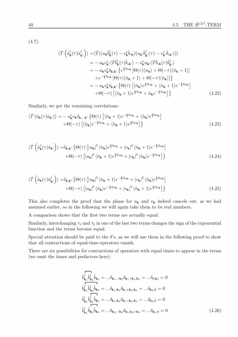
40 4.5. THE H(3)2-TERM
(4.7):
〈T(a†k(τ)a
†k′
)〉 =〈T ((ukb
†k(τ)− v∗kb-k)(uk′ b†
k′(τ)− v∗k′ b-k′))〉
=− ukv∗k′〈T b†k(τ)b-k′〉 − v∗kuk′〈T b-k(τ)b†k′〉
=− ukv∗kδk,k′
e
τ~~ωk [Θ(τ)〈nk〉+Θ(−τ)〈nk + 1〉]
+e−τ~~ωk [Θ(τ)〈nk + 1〉+Θ(−τ)〈nk〉]
=− ukv∗kδk,k′
Θ(τ)
[〈nk〉e
τ~~ωk + 〈nk + 1〉e− τ
~~ωk
]
+Θ(−τ)[〈nk + 1〉e τ
~~ωk + nke
− τ~~ωk
](4.22)
Similarly, we get the remaining correlations:
〈T (ak(τ)ak′)〉 =− u∗kvkδk,−k′
Θ(τ)
[〈nk + 1〉e− τ
~~ωk + 〈nk〉e
τ~~ωk
]
+Θ(−τ)[〈nk〉e−
τ~~ωk + 〈nk + 1〉e τ
~~ωk
](4.23)
〈T(a†k(τ)ak′
)〉 =δk,k′
Θ(τ)
[|uk|2 〈nk〉e
τ~~ωk + |vk|2 〈nk + 1〉e− τ
~~ωk
]
+Θ(−τ)[|uk|2 〈nk + 1〉e τ
~~ωk + |vk|2 〈nk〉e−
τ~~ωk
](4.24)
〈T(ak(τ)a
†k′
)〉 =δk,k′
Θ(τ)
[|uk|2 〈nk + 1〉e− τ
~~ωk + |vk|2 〈nk〉e
τ~~ωk
]
+Θ(−τ)[|uk|2 〈nk〉e−
τ~~ωk + |vk|2 〈nk + 1〉e τ
~~ωk
](4.25)
This also completes the proof that the phase for uk and vk indeed cancels out, as we hadassumed earlier, so in the following we will again take them to be real numbers.
A comparison shows that the first two terms are actually equal.
Similarly, interchanging τ1 and τ2 in one of the last two terms changes the sign of the exponentialfunction and the terms become equal.
Special attention should be paid to the δ′s, as we will use them in the following proof to showthat all contractions of equal-time-operators vanish.
There are six possibilities for contractions of operators with equal times to appear in the terms(we omit the times and prefactors here):
b†k1b†k2
bk3 = ...δk1,−k2δk1+k2,k3 = ...δ0,k3 = 0
b†k1b†k2
bk3 = ...δk1,k3δk1+k2,k3 = ...δk2,0 = 0
b†k1b†k2
bk3= ...δk1,k3δk1+k2,k3 = ...δk2,0 = 0
b†k1bk2 bk3 = ...δk2,−k3δk1,k2+k3 = ...δk1,0 = 0 (4.26)

CHAPTER 4. BEYOND THE BOGOLIUBOV APPROXIMATION: SECOND ORDER 41
b†k1bk2 bk3 = ...δk1,k2δk1,k2+k3 = ...δ0,k3 = 0
b†k1bk2 bk3 = ...δk1,k3δk1,k2+k3 = ...δ0,k2 = 0
This leaves us with just six expressions for each of the four terms, 24 altogether. The very firstthought of reducing the number of terms is to check whether we can halve the terms by per-muting two k’s, since at τ1 and τ2 there are always two creation or two annihilation operators.We must not forget the original δ but it is easily seen that halving the terms is possible becauseone always finds two terms with the same δ. The twelve terms can be reduced even further,but this will be done in the next chapter where it can be visually seen which terms are equal.We will take a little different approach than in the last chapter, since directly inserting the b′kswould lead to a plethora of terms. Instead, we write down the expressions in terms of the a′ks,
calculate the arising contractions and only then change to the b′ks . The second column liststhe possible renaming of the variables, one for each of the twelve terms. The others are thecontracted operators and the last row shows all δ′s for each term. As before, we observe thatone of the original δ’s just acts as the unity operator, for example in the first term:δk1,-k4 δk2,-k5 δk3,-k6 δk1+k2,k3 δk4+k5,k6 = δk1,-k4 δk2,-k5 δk3,-k6 δk1+k2,k3 δ-k1-k2,-k3
1.
ak4 ↔ ak5
a†k1a†k4 a†k2a
†k5 ak3ak6 δk1,-k4 δk2,-k5 δk3,-k6 δk1+k2,k3
2. a†k1a†k4 a†k2ak6 ak3a
†k5 δk1,-k4 δk2,k6 δk3,k5 δk1+k2,k3
3. a†k1ak6 a†k2a†k4 ak3a
†k5 δk1,k6 δk2,-k4 δk3,k5 δk1+k2,k3
4.
ak5 ↔ ak6
a†k1a†k4 a†k2ak5 ak3ak6 δk1,-k4 δk2,k5 δk3,-k6 δk1+k2,k3
5. a†k1ak6 a†k2ak5 ak3a†k4 δk1,k6 δk2,k5 δk3,k4 δk1+k2,k3
6. a†k1ak6 a†k2a†k4 ak3ak5 δk1,k6 δk2,-k4 δk3,-k5 δk1+k2,k3
7.
ak4 ↔ ak5
a†k1a†k4 ak2a
†k5 ak3ak6 δk1,-k4 δk2,k5 δk3,-k6 δk1,k2+k3
8. a†k1a†4 ak2ak6 ak3a
†k5 δk1,-k4 δk2,-k6 δk3,k5 δk1,k2+k3
9. a†k1ak6 ak2a†k4 ak3a
†k5 δk1,k6 δk2,k4 δk3,k5 δk1,k2+k3
10.
ak5 ↔ ak6
a†k1a†k4 ak2ak5 ak3ak6 δk1,-k4 δk2,-k5 δk3,-k6 δk1,k2+k3
11. a†k1a6 ak2ak5 ak3a†k4 δk1,k6 δk2,-k5 δk3,k4 δk1,k2+k3
12. a†k1ak6 ak2a†k4 ak3ak5 δk1,k6 δk2,k4 δk3,-k5 δk1,k2+k3
One can show that these 12 remaining terms can again be reduced to only four different expres-sions, using that several contractions are equal, as seen on page 40.By interchanging k1 and k2,the second and third and the fourth and sixth expression can be seen to be equal, respectively.Similarly, by replacing k2 with k3 in the 7th and 8th as well as in the 11th and 12th term one getsthe same expression also. We have to take care if this stays correct for the original δ′s, whichis indeed the case as can be read off from the above table. The remaining four identificationsare listed.
• The fourth and seventh term are equal by changing τ1 τ2 as well as k1 and k3 in theseventh term.
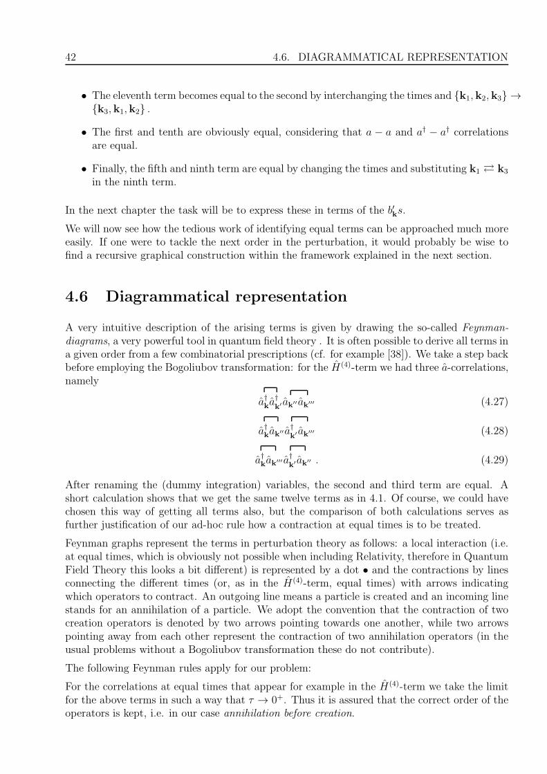
42 4.6. DIAGRAMMATICAL REPRESENTATION
• The eleventh term becomes equal to the second by interchanging the times and k1,k2,k3 →k3,k1,k2 .
• The first and tenth are obviously equal, considering that a − a and a† − a† correlationsare equal.
• Finally, the fifth and ninth term are equal by changing the times and substituting k1 k3
in the ninth term.
In the next chapter the task will be to express these in terms of the b′ks.
We will now see how the tedious work of identifying equal terms can be approached much moreeasily. If one were to tackle the next order in the perturbation, it would probably be wise tofind a recursive graphical construction within the framework explained in the next section.
4.6 Diagrammatical representation
A very intuitive description of the arising terms is given by drawing the so-called Feynman-diagrams, a very powerful tool in quantum field theory . It is often possible to derive all terms ina given order from a few combinatorial prescriptions (cf. for example [38]). We take a step backbefore employing the Bogoliubov transformation: for the H(4)-term we had three a-correlations,namely
a†ka†k′ ak′′ ak′′′ (4.27)
a†kak′′ a†k′ ak′′′ (4.28)
a†kak′′′ a†k′ ak′′ . (4.29)
After renaming the (dummy integration) variables, the second and third term are equal. Ashort calculation shows that we get the same twelve terms as in 4.1. Of course, we could havechosen this way of getting all terms also, but the comparison of both calculations serves asfurther justification of our ad-hoc rule how a contraction at equal times is to be treated.
Feynman graphs represent the terms in perturbation theory as follows: a local interaction (i.e.at equal times, which is obviously not possible when including Relativity, therefore in QuantumField Theory this looks a bit different) is represented by a dot • and the contractions by linesconnecting the different times (or, as in the H(4)-term, equal times) with arrows indicatingwhich operators to contract. An outgoing line means a particle is created and an incoming linestands for an annihilation of a particle. We adopt the convention that the contraction of twocreation operators is denoted by two arrows pointing towards one another, while two arrowspointing away from each other represent the contraction of two annihilation operators (in theusual problems without a Bogoliubov transformation these do not contribute).
The following Feynman rules apply for our problem:
For the correlations at equal times that appear for example in the H(4)-term we take the limitfor the above terms in such a way that τ → 0+. Thus it is assured that the correct order of theoperators is kept, i.e. in our case annihilation before creation.
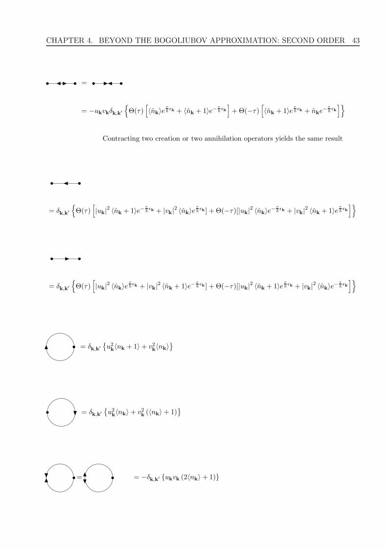
CHAPTER 4. BEYOND THE BOGOLIUBOV APPROXIMATION: SECOND ORDER 43
=
= −ukvkδk,k′
Θ(τ)
[〈nk〉e
τ~ǫk + 〈nk + 1〉e− τ
~ǫk]+Θ(−τ)
[〈nk + 1〉e τ
~ǫk + nke
− τ~ǫk]
Contracting two creation or two annihilation operators yields the same result
= δk,k′
Θ(τ)
[|uk|2 〈nk + 1〉e− τ
~ǫk + |vk|2 〈nk〉e
τ~ǫk ] + Θ(−τ)[|uk|2 〈nk〉e−
τ~ǫk + |vk|2 〈nk + 1〉e τ
~ǫk]
= δk,k′
Θ(τ)
[|uk|2 〈nk〉e
τ~ǫk + |vk|2 〈nk + 1〉e− τ
~ǫk ] + Θ(−τ)[|uk|2 〈nk + 1〉e τ
~ǫk + |vk|2 〈nk〉e−
τ~ǫk]
= δk,k′
u2k〈nk + 1〉+ v2k〈nk〉
= δk,k′
u2k〈nk〉+ v2k (〈nk〉+ 1)
= = −δk,k′ ukvk (2〈nk〉+ 1)
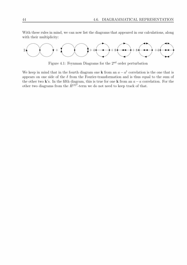
44 4.6. DIAGRAMMATICAL REPRESENTATION
With these rules in mind, we can now list the diagrams that appeared in our calculations, alongwith their multiplicity:
2 + + 4 + 8 + 8 +4
Figure 4.1: Feynman Diagrams for the 2nd order perturbation
We keep in mind that in the fourth diagram one k from an a− a† correlation is the one that isappears on one side of the δ from the Fourier-transformation and is thus equal to the sum ofthe other two k’s. In the fifth diagram, this is true for one k from an a− a correlation. For theother two diagrams from the H(3)2-term we do not need to keep track of that.
Chapter 5
Calculations with the second orderapproximation
”Always try to innovate. If you lose your old fitness, you lose out to Bose-Einstein condensation. I am
sure that companies that go under would feel better if they knew that they were victims of Bose-Einstein
condensation.”
Prof. Jennifer Tour Chayes at the MAA 2007 Hedrick Lecture
After having collected all terms in second loop-order, we can in a similar manner as in thepreceding chapters, again calculate the Effective Hamiltonian and the Free Energy. From thiswe can ultimately calculate the particle density that can be checked for a phase transition aswell as be used to plot the time-of-flight pictures. In complete analogy to the proceedings inchapter 3 and 4 we first write down the effective potential as
Veff = − 1
βlnZ = − 1
βln
(Z0
Z
Z0
)= − 1
βlnZ0 −
1
βln
Z
Z0
. (5.1)
The first term is just V(0)eff , the effective potential for the diagonalized Hamiltonian. The ex-
pansion of ZZ0
is given in eq. 4.5. In short notation without the sums and integrals we thus get
(keeping in mind that the perturbation here is H(3) + H(4):
lnZ
Z0
= ln
1− 1
~
(H(3) + H(4)
)+
1
~2
(H(3) + H(4)
)2+ ...
(5.2)
We have the Taylor-expansion ln (1 + x) ≈ x − x2
2, which we do not calculate here as we have
already convinced ourselves that only H(4) and H(3)2 constitute the second loop order; allremaining terms are either zero or from a higher order.
5.1 The zero-temperature limit
We have already reduced the number of different terms considerably, still there are definitelytoo many to write them all down or try to go ahead and calculate the Free Energy. Therefore,at this point we already carry out the zero-temperature limit T → 0. Since so far no way of
45
46 5.1. THE ZERO-TEMPERATURE LIMIT
measuring the temperature of a BEC has been found, we would have taken this limit anywaysomewhere along the line.
Let us therefore for now only concentrate on the dependency on T or, equivalently β.
In the H(4)-term the time-dependence of the operators, as mentioned, cancels out and theone time-integral just gives ~β. This just cancels out with the − 1
βfrom the definition of
the Effective Potential, so the temperature-dependency is only present in the 〈nk〉 ’s. Sincelimβ→∞〈nk〉 = limβ→∞
1eβ~ωk
= 0, only those terms survive that do not include an 〈nk〉. Fromthe first diagram (neglecting other prefactors and sums) we thus only have a term with v2kv
2k′
and from the second also only one term with ukvkuk′vk′ .
The other terms are a little more involved: in eqs. 4.22 ff. we see the time-dependent correla-tions. In the H(3)2-term all arising terms contain three a-correlations, all with τ1 and τ2.
We would now like to see correlations in the four Feynman-diagrams expressed via the bk’s.Luckily, by a few considerations we can substantially reduce the number of arising terms.We see that each contraction consists of a term with Θ(τ) or a Θ(−τ). From the properties ofHeaviside-functions it follows that multiplying the same Θ′s is just again the Heaviside-functionwhile multiplying two with a different sign of the argument yields zero. That still leaves quitea lot of terms, so let us now take the zero-temperature limit to simplify these.
At first we shall have a look at the simple a− a correlations and then see how we can translatethose results to the actual terms that appear in perturbation theory. We see that the β-dependence manifests itself in one of four different possible combinations:
1.∫ ~β
0
∫ ~β
0Θ(τ1 − τ2)e
~ωk(τ1−τ2)〈nk〉dτ1dτ2
2.∫ ~β
0
∫ ~β
0Θ(τ1 − τ2)e
~ωk(τ2−τ1)〈nk + 1〉dτ1dτ2
3.∫ ~β
0
∫ ~β
0Θ(τ2 − τ1)e
~ωk(τ1−τ2)〈nk + 1〉dτ1dτ2
4.∫ ~β
0
∫ ~β
0Θ(τ2 − τ1)e
~ωk(τ2−τ1)〈nk〉dτ1dτ2
First of all, we see that the first and fourth as well as the second and third term are actuallythe same, so we analyze the two different terms by use of the integrals
~β∫
0
~β∫
0
Θ(τ1 − τ2)eωk(τ1−τ2)dτ1dτ2 =
~β∫
0
eωkτ1dτ2
τ1∫
0
e−ωkτ2dτ2 =1
ωk
~β∫
0
eωkτ1(1− e−ωτ1
)dτ1
=1
ωk
~β∫
0
(eωkτ1 − 1) = −~β
ωk
+1
ω2k
(e~ωkβ − 1
)
and~β∫
0
~β∫
0
Θ(τ2 − τ1)eωk(τ1−τ2)dτ1dτ2 =
~β
ωk
+1
ω2k
(e−~ωkβ − 1
).
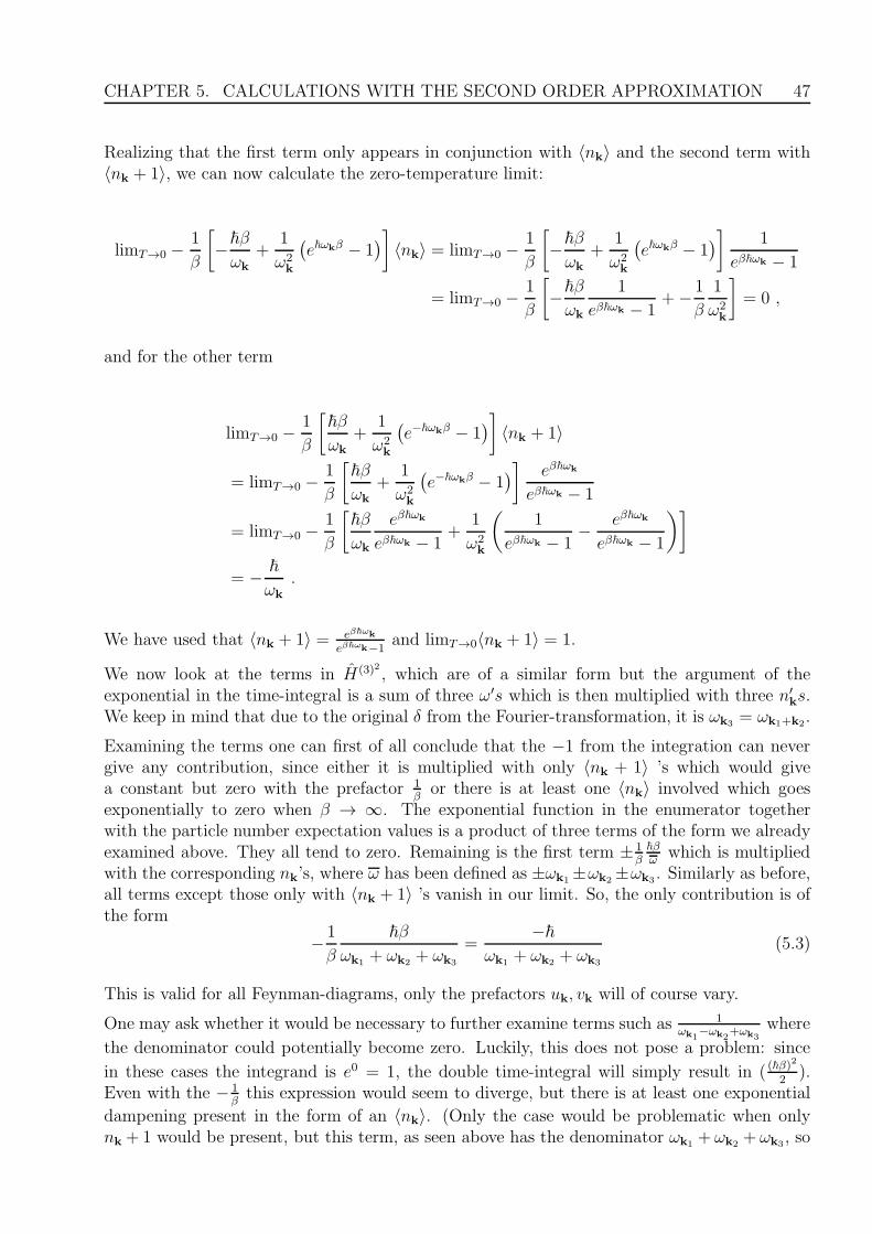
CHAPTER 5. CALCULATIONS WITH THE SECOND ORDER APPROXIMATION 47
Realizing that the first term only appears in conjunction with 〈nk〉 and the second term with〈nk + 1〉, we can now calculate the zero-temperature limit:
limT→0 −1
β
[−~β
ωk
+1
ω2k
(e~ωkβ − 1
)]〈nk〉 = limT→0 −
1
β
[−~β
ωk
+1
ω2k
(e~ωkβ − 1
)] 1
eβ~ωk − 1
= limT→0 −1
β
[−~β
ωk
1
eβ~ωk − 1+− 1
β
1
ω2k
]= 0 ,
and for the other term
limT→0 −1
β
[~β
ωk
+1
ω2k
(e−~ωkβ − 1
)]〈nk + 1〉
= limT→0 −1
β
[~β
ωk
+1
ω2k
(e−~ωkβ − 1
)] eβ~ωk
eβ~ωk − 1
= limT→0 −1
β
[~β
ωk
eβ~ωk
eβ~ωk − 1+
1
ω2k
(1
eβ~ωk − 1− eβ~ωk
eβ~ωk − 1
)]
= − ~
ωk
.
We have used that 〈nk + 1〉 = eβ~ωk
eβ~ωk−1and limT→0〈nk + 1〉 = 1.
We now look at the terms in H(3)2 , which are of a similar form but the argument of theexponential in the time-integral is a sum of three ω′s which is then multiplied with three n′
ks.We keep in mind that due to the original δ from the Fourier-transformation, it is ωk3 = ωk1+k2.
Examining the terms one can first of all conclude that the −1 from the integration can nevergive any contribution, since either it is multiplied with only 〈nk + 1〉 ’s which would givea constant but zero with the prefactor 1
βor there is at least one 〈nk〉 involved which goes
exponentially to zero when β → ∞. The exponential function in the enumerator togetherwith the particle number expectation values is a product of three terms of the form we alreadyexamined above. They all tend to zero. Remaining is the first term ± 1
β~βω
which is multipliedwith the corresponding nk’s, where ω has been defined as ±ωk1 ±ωk2 ±ωk3 . Similarly as before,all terms except those only with 〈nk + 1〉 ’s vanish in our limit. So, the only contribution is ofthe form
− 1
β
~β
ωk1 + ωk2 + ωk3
=−~
ωk1 + ωk2 + ωk3
(5.3)
This is valid for all Feynman-diagrams, only the prefactors uk, vk will of course vary.
One may ask whether it would be necessary to further examine terms such as 1ωk1
−ωk2+ωk3
where
the denominator could potentially become zero. Luckily, this does not pose a problem: since
in these cases the integrand is e0 = 1, the double time-integral will simply result in ( (~β)2
2).
Even with the − 1βthis expression would seem to diverge, but there is at least one exponential
dampening present in the form of an 〈nk〉. (Only the case would be problematic when onlynk + 1 would be present, but this term, as seen above has the denominator ωk1 + ωk2 + ωk3 , so
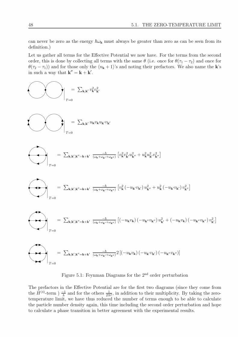
48 5.1. THE ZERO-TEMPERATURE LIMIT
can never be zero as the energy ~ωk must always be greater than zero as can be seen from itsdefinition.)
Let us gather all terms for the Effective Potential we now have. For the terms from the secondorder, this is done by collecting all terms with the same θ (i.e. once for θ(τ1 − τ2) and once forθ(τ2 − τ1)) and for those only the 〈nk + 1〉’s and noting their prefactors. We also name the k’sin such a way that k′′ = k + k′.
T=0
=∑
k,k′ v2kv2k′
T=0
=∑
k,k′ ukvkuk′vk′
T=0
=∑
k,k′,k′′=k+k′−~
(ωk+ωk′+ω
k′′ )
[v2kv
2k′u2
k′′ + u2ku
2k′v2k′′
]
T=0
=∑
k,k′,k′′=k+k′−~
(ωk+ωk′+ω
k′′ )
[v2k (−uk′vk′)u2
k′′ + u2k (−uk′vk′) v2
k′′
]
T=0
=∑
k,k′,k′′=k+k′−~
(ωk+ωk′+ω
k′′ )
[(−ukvk) (−uk′′vk′′)u2
k′ + (−ukvk) (−uk′′vk′′) v2k′
]
T=0
=∑
k,k′,k′′=k+k′−~
(ωk+ωk′+ω
k′′)2 [(−ukvk) (−uk′vk′) (−uk′′vk′′)]
Figure 5.1: Feynman Diagrams for the 2nd order perturbation
The prefactors in the Effective Potential are for the first two diagrams (since they come fromthe H(4)-term ) −1
~and for the others 1
2!~2, in addition to their multiplicity. By taking the zero-
temperature limit, we have thus reduced the number of terms enough to be able to calculatethe particle number density again, this time including the second order perturbation and hopeto calculate a phase transition in better agreement with the experimental results.
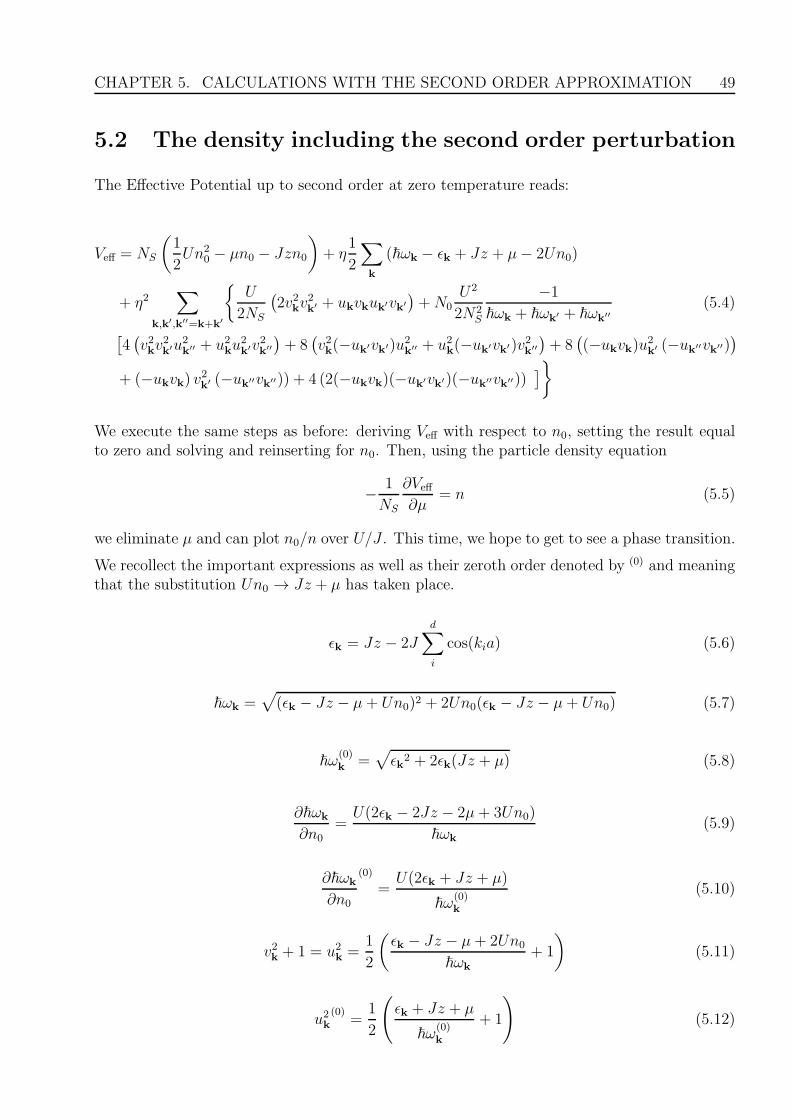
CHAPTER 5. CALCULATIONS WITH THE SECOND ORDER APPROXIMATION 49
5.2 The density including the second order perturbation
The Effective Potential up to second order at zero temperature reads:
Veff = NS
(1
2Un2
0 − µn0 − Jzn0
)+ η
1
2
∑
k
(~ωk − ǫk + Jz + µ− 2Un0)
+ η2∑
k,k′,k′′=k+k′
U
2NS
(2v2kv
2k′ + ukvkuk′vk′
)+N0
U2
2N2S
−1
~ωk + ~ωk′ + ~ωk′′
(5.4)
[4(v2kv
2k′u2
k′′ + u2ku
2k′v2k′′
)+ 8
(v2k(−uk′vk′)u2
k′′ + u2k(−uk′vk′)v2k′′
)+ 8
((−ukvk)u
2k′ (−uk′′vk′′)
)
+ (−ukvk) v2k′ (−uk′′vk′′)) + 4 (2(−ukvk)(−uk′vk′)(−uk′′vk′′))
]
We execute the same steps as before: deriving Veff with respect to n0, setting the result equalto zero and solving and reinserting for n0. Then, using the particle density equation
− 1
NS
∂Veff
∂µ= n (5.5)
we eliminate µ and can plot n0/n over U/J . This time, we hope to get to see a phase transition.
We recollect the important expressions as well as their zeroth order denoted by (0) and meaningthat the substitution Un0 → Jz + µ has taken place.
ǫk = Jz − 2Jd∑
i
cos(kia) (5.6)
~ωk =√(ǫk − Jz − µ+ Un0)2 + 2Un0(ǫk − Jz − µ+ Un0) (5.7)
~ω(0)k =
√ǫk2 + 2ǫk(Jz + µ) (5.8)
∂~ωk
∂n0=
U(2ǫk − 2Jz − 2µ+ 3Un0)
~ωk
(5.9)
∂~ωk
∂n0
(0)
=U(2ǫk + Jz + µ)
~ω(0)k
(5.10)
v2k + 1 = u2k =
1
2
(ǫk − Jz − µ+ 2Un0
~ωk
+ 1
)(5.11)
u2k
(0)=
1
2
(ǫk + Jz + µ
~ω(0)k
+ 1
)(5.12)
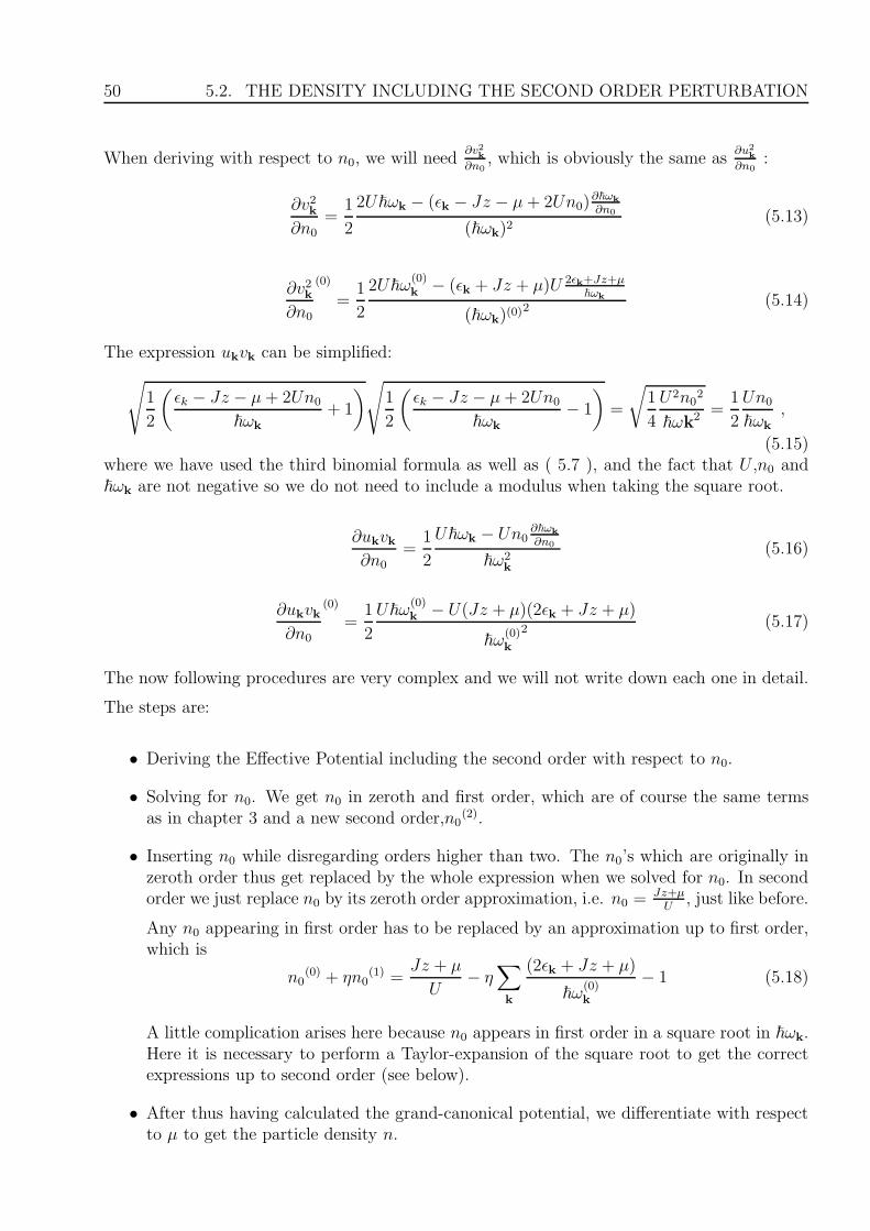
50 5.2. THE DENSITY INCLUDING THE SECOND ORDER PERTURBATION
When deriving with respect to n0, we will need∂v2
k
∂n0, which is obviously the same as
∂u2k
∂n0:
∂v2k∂n0
=1
2
2U~ωk − (ǫk − Jz − µ+ 2Un0)∂~ωk
∂n0
(~ωk)2(5.13)
∂v2k∂n0
(0)
=1
2
2U~ω(0)k − (ǫk + Jz + µ)U 2ǫk+Jz+µ
~ωk
(~ωk)(0)2 (5.14)
The expression ukvk can be simplified:
√1
2
(ǫk − Jz − µ+ 2Un0
~ωk
+ 1
)√1
2
(ǫk − Jz − µ+ 2Un0
~ωk
− 1
)=
√1
4
U2n02
~ωk2 =1
2
Un0
~ωk
,
(5.15)where we have used the third binomial formula as well as ( 5.7 ), and the fact that U ,n0 and~ωk are not negative so we do not need to include a modulus when taking the square root.
∂ukvk∂n0
=1
2
U~ωk − Un0∂~ωk
∂n0
~ω2k
(5.16)
∂ukvk∂n0
(0)
=1
2
U~ω(0)k − U(Jz + µ)(2ǫk + Jz + µ)
~ω(0)k
2 (5.17)
The now following procedures are very complex and we will not write down each one in detail.
The steps are:
• Deriving the Effective Potential including the second order with respect to n0.
• Solving for n0. We get n0 in zeroth and first order, which are of course the same termsas in chapter 3 and a new second order,n0
(2).
• Inserting n0 while disregarding orders higher than two. The n0’s which are originally inzeroth order thus get replaced by the whole expression when we solved for n0. In secondorder we just replace n0 by its zeroth order approximation, i.e. n0 =
Jz+µU
, just like before.
Any n0 appearing in first order has to be replaced by an approximation up to first order,which is
n0(0) + ηn0
(1) =Jz + µ
U− η
∑
k
(2ǫk + Jz + µ)
~ω(0)k
− 1 (5.18)
A little complication arises here because n0 appears in first order in a square root in ~ωk.Here it is necessary to perform a Taylor-expansion of the square root to get the correctexpressions up to second order (see below).
• After thus having calculated the grand-canonical potential, we differentiate with respectto µ to get the particle density n.
CHAPTER 5. CALCULATIONS WITH THE SECOND ORDER APPROXIMATION 51
• Solving this equation for the chemical potential and again reinserting, we can eliminateµ.
• By setting n = 1 (one could also choose another density) we can proceed to plot theequation
n− n0 = f(n, U/J) (5.19)
and hope for a solution, meaning that n0 → 0 for a particular value of the experimentalparameters U/J which could of course be compared to the experiment.
Unfortunately, after having done all these things, we encountered a surprising problem: in theterms appear infrared divergencies, obviously a problem when we turn from sums to integralswhich run over the zero. This problem was also encountered in [39] when calculating the secondorder perturbation theory via the formulism of path integrals.
This means we will have to be content to prove the existence of these divergencies and therebyshow that the method of reinserting unfortunately is not feasible. For brevity, we will omit inthe following calculations the contribution from the H(3)2-term. It can easily be seen that thoseomitted terms cannot cancel out the divergencies we write down now, because the rest. So, ifwe encounter divergencies in the rest, the whole Hamiltonian has to have them.
Veff = NS
(1
2Un2
0 − µn0 − Jzn0
)+ η
1
2
∑
k
(~ωk − ǫk + Jz + µ− 2Un0)
+ η2∑
k,k′,k′′=k+k′
U
2NS
(2v2kv
2k′ + ukvkuk′vk′
)(5.20)
n0 has to be inserted basically in five different places: in the first one it needs to be squared,so we get
(n0(0) + ηn0
(1) + η2n0(2))
2= n0
(0)2 + 2ηn0(0)n0
(1) + η2n0(1)2 + 2η2n0
(0)n0(2) +O(η3) . (5.21)
Depending on the place of the n0, the zeroth, first, or second order approximation has to beinserted. We have
n0(2) = −1
2
∑
k
∂~ωk
∂n0
(1)
− 1
2
∑
k
∑
k′
2(∂vk
2
∂n0
vk′2 +
∂vk′2
∂n0
vk2) +
∂ukvk∂n0
uk′vk′ +∂uk′vk′
∂n0
ukvk
= −1
2
∑
k
∂~ωk
∂n0
(1)
−∑
k
∑
k′
2∂vk
2
∂n0vk′
2 +∂ukvk∂n0
uk′vk′ , (5.22)
where we have used that Un0(0) = Jz + µ.
The square root appearing in the ~ωk in first order has to be expanded up to first order, yielding
52 5.2. THE DENSITY INCLUDING THE SECOND ORDER PERTURBATION
√(ǫk + ηn0
(1))2+ 2U(n0
(0) + ηn0(1))(ǫk + ηUn0
(1))
=√
ǫk2 + 2ǫkUn0(0) + η
2ǫkn0(1)U + n0
(0)n0(1)U2
√ǫk2 + 2ǫkUn0
(0)
= ~ωk(0) + η
2ǫkn0(1)U + n0
(0)n0(1)U2
~ωk(0)
. (5.23)
Similarly, we perform an expansion of ∂~ωk
∂n0:
∂~ωk
∂n0
(1)
= U2(2ǫk′ + Un0
˜~2ωk′(0)
− 1)ǫk − Un0
~ωk(0)
3 (5.24)
One should take care that the sum which appears in n0(1) needs to run over a index different
from k.
With that, we can write down the grand-canonical potential. We limit ourselves to the secondorder, the zeroth and first remain the same as in the earlier chapters, of course.
Ω(2) =1
2Un0
(1)2 +1
2
∑
k
[~ωk(1) − 2Un0
(1)] +U
2
∑
k
∑
k′
2v2k(0)u2k′
(0)+ ukvk
(0)uk′vk′(0) (5.25)
Interestingly, n0(2) cancels out in Ω, which is very convenient since that means we will not need
the derivatives of H(4).
In the next step, we take the derivatives with respect to the chemical potential in order to solvefor the particle density. When reinserting, we use a tilde,”˜”, to denote the result, so as not tocreate a confusion with ”(0)”.
∂~ωk(0)
∂µ=
ǫk
~ωk(0)
(5.26)
~ωk(0) =
√ǫk2 + 2ǫkUn (5.27)
∂ukvk(0)
∂µ=
1
2
U
~ωk(0)
(1− Un
ǫ2k + 2ǫkUn) (5.28)
∂˜vk2(0)
∂µ=
1
2~ωk(0)
(1− ǫk2 + ǫkUn
ǫ2k + 2ǫkUn) (5.29)
∂˜~ωk(1)
∂µ= −U
ǫk′(2ǫk + Un)(−ǫk′ + Un)
2~ωk~ωk′3 −U
ǫk(2ǫk + Un)(1− 2ǫk′+Un
2~ωk
)
~ωk3 +U
1− 2ǫk′+Un
~ωk′
~ωk
(5.30)
CHAPTER 5. CALCULATIONS WITH THE SECOND ORDER APPROXIMATION 53
We will now examine the behavior for small k, i.e. the infrared domain.
We begin with ǫk, which was basically 1− cos(k), which, as we remarked earlier, results in thek2-behavior of ǫk for small k.
For ~ωk(0) we can therefore observe a linear dependency on k for small k:
√ǫk√
ǫk + Un ∼√k2√k2 + const. ∼ k (5.31)
n0(1) ∼ ǫk + 2Un
~ωk(0)
− 1 ∼ k +1
k+ const. ∼ 1
k(5.32)
∂n0(1)
∂µ∼ 1
~ωk(0)
ǫk(ǫk + 2Un)
~ωk(0)
∼ k3 + k +1
k+ const. ∼ 1
k(5.33)
ukvk(0) ∼Un
~ωk(0)
∼ 1
k(5.34)
∂ukvk(0)
∂µ∼ 1
~ωk(0)
(1− Un
ǫk2 + 2Un) ∼ 1
k(1− 1
k4 + 1) ∼ 1
k(5.35)
˜vk2(0) ∼ ǫk + Un
~ωk(0)
− 1 ∼ k2 + const.
k+ const. ∼ 1
k(5.36)
∂ ˜vk2(0)
∂µ∼ 1
~ωk(0)
(1− ǫk2 + ǫkUn
ǫ2k + 2ǫkUn) ∼ 1
k(const.− k4 + k2
k4 + k2) ∼ 1
k(5.37)
And, finally
∂˜~ωk(1)
∂µ=
ǫk′(2ǫk + Un)(−ǫk′ + Un)
2~ωk~ωk′3 − U
ǫk(2ǫk + Un)(1 − 2ǫk′+Un
2~ωk
)
~ωk3 + U
1− 2ǫk′+Un
~ωk′
~ωk
∼ k′2(k2 + const.)(k′2 + const.)
kk′3− k(k2 + const.)(1− k′+const.
k)
k3+
1− k′2+const.k′
k
∼ 1
kk′− 1
kk′+
1
kk′∼ 1
kk′. (5.38)
Looking back at 5.25, we see that k and k’, respectively, diverge at most linearly. This does notpresent a problem, since when integrating and switching to spherical coordinates, we get fromthe Jacobian a k2 (or k′2), so the integrals possess a finite value.
So far, the calculated terms do not give any divergencies. Problems arise only when taking thederivatives ∂vk
2
∂n0and ∂vkuk
∂n0, which we will show now.
We have the needed derivatives already calculated, see 5.17, 5.14 and 5.24.
Eliminating µ (here we simply need to insert the lowest order) yields
54 5.2. THE DENSITY INCLUDING THE SECOND ORDER PERTURBATION
∂ukvk(0)
∂n0=
1
2(
U
~ωk(0)
− U2n(2ǫk + Un)
~ωk(0)
3 ) (5.39)
∂vk(0)2
∂n0=
1
2(
2U
~ωk(0)
− (ǫk + Un)U(2ǫk + Un)
~ωk(0)
3 ) (5.40)
and
∂˜~ωk(1)
∂n0
= U2(2ǫk′ + Un
˜2~ωk′(0)
− 1)ǫk − Un2
~ωk(0)
3 . (5.41)
We have the product of two vk2’s and two ukvk’s so when deriving and renaming we get twice
the product where one part has been derived. We also include all the prefactors from ??,resulting in the three terms:
−1
222vk
2∂vk′2
∂n0= −2
1
2(ǫk + Un
~ωk
− 1)1
2
[2U
~ωk′
− (ǫk′ + Un)U(2ǫk′ + Un)
~ωk′3
](5.42)
−1
22ukvk
∂uk′vk′
∂n0
= − Un
2~ωk
1
2
[U
~ωk′
− U2n(2ǫk′ + Un)
~ωk′3
](5.43)
− 1
2U
∂~ωk(1)
∂n0= −−Unk′
(1)(ǫk − Un)2
~ωk3 (5.44)
From these three equations we extract the ”problematic” terms, i.e. those which diverge witha power greater than two. This only happens where the third power of ~ω appears in thedenominator.
1
2(ǫk + Un
~ωk
− 1)−U3n2
~ωk′3
1
4
Un
~ωk
U3n2
~ωk′3 (5.45)
1
2
U3n2
~ωk3 (
−2ǫk′ − Un
2~ωk′
+ 1)
where the last factor in the third equation is nk′(1).
Although the terms look very similar (when swapping the variables in the third equation), theyunfortunately do not quite cancel each other out, we get stuck with
U4n2
2~ωk~ωk′3 (5.46)
so we see that the term is divergent, at least in one variable.
With that, we have shown that our original ansatz unfortunately cannot lead to a useful ap-proximation in second order. One possible solution could be to just cancel the divergent term,viewing it as ”unphysical”. We decided not to do that.
CHAPTER 5. CALCULATIONS WITH THE SECOND ORDER APPROXIMATION 55
5.3 Can Popov help us?
Maybe the variational ansatz µ → M + η∆ can help us once again, as it did before.
Unfortunately, no. Inserting the relation above in Ω cf. 3.64 yields for the lowest order:
−NS
2U(Jz + µ)2 → −NS
2U(Jz +M + η∆)2 (5.47)
Consequently, deriving yields:
∂(Jz +M + η∆)2
∂M= 2(Jz +M + η∆) (5.48)
With the elimination of ∆ via ∆ = µ−MM
we see that M does not appear anymore. Therefore,we are unable to solve for M and reinsert.
The situation was different when we only included the first order, because then we actuallydiscarded a term in the quadratic µ. VPT thus will not help us here, we have to concede atthis point that we will not be able to get a result for the second order.

56 5.3. CAN POPOV HELP US?
Chapter 6
Calculations without reinserting
”I wish to God these calculations had been executed by steam.”
Charles Babbage
6.1 Why we cannot see a phase transition
We now show that the condition ∂Veff
∂n0for n0 does not have a solution for n0 = 0 when reinserting.
(Since both equations have to be satisfied for a solution, our whole system of equations cannothave a solution.)
When deriving and going to n0 → 0 we encounter the problem, for example in ~ωk, that wehave to take the root of a square which results in the modulus if negative values are possible:
√(ǫk − Jz − µ)2 = |ǫk − Jz − µ| (6.1)
Taking all the derivatives, then taking the limit of a vanishing condensate density yields
expression expression taken at n0 = 0 |ǫk − Jz − µ| > 0 |ǫk − Jz − µ| < 0
~ωk |ǫk − Jz − µ| ǫk − Jz − µ −(ǫk − Jz − µ)
∂~ωk
∂n02U ǫk−Jz−µ
|ǫk−Jz−µ|2U −2U
uk2 1
2( ǫk−Jz−µ|ǫk−Jz−µ|
+ 1) 1 0
vk2 1
2( ǫk−Jz−µ|ǫk−Jz−µ|
− 1) 0 -1
∂uk2
∂n0= ∂vk
2
∂n0
12( 2U|ǫk−Jz−µ|
− ǫk−Jz−µ
|ǫk−Jz−µ|22U ǫk−Jz−µ
|ǫk−Jz−µ|) 0 0
ukvk 0 0 0
∂ukvk∂n0
U2|ǫk−Jz−µ|
U2ǫk−Jz−µ
−U2ǫk−Jz−µ
So, we see that any term that includes as a factor ukvk or ∂uk2
∂n0, (or ∂vk
2
∂n0) goes to zero when n0
goes to zero.
57
58 6.2. NUMERICAL CALCULATIONS
Thus we see that the derivative of H(4) becomes zero for n0 → 0.
The H(3)2-term is a little bit more involved: since it is multiplied with n0, the derivative is ofthe form (...) + n0
∂(...)∂n0
. The second part is zero, what about the first?
It consists of a product of 1~ωk+~ω
k′+~ωk′′and 7 terms, divided in 4 subgroups. These groups are
(without prefactors):
I. v2kv2k′u2
k′′ + u2ku
2k′v2k′′
II. v2k(−uk′vk′)u2k′′ + u2
k(−uk′vk′)v2k′′
III. (−ukvk)u2k′(−uk′′vk′′) + (−ukvk)v
2k′(−uk′′vk′′)
IV. (−ukvk)(−uk′vk′)(−uk′′vk′′)
Let us first look at the terms which are derived: in I, each term in the derivative has to include
either∂v2
k
∂n0or
∂u2k
∂n0which means, as was just proved, that they are all zero.
In II, we have either again the derivatives as in I that make it go to zero, but we also have thepart where only the ukvk gets derived. But, we have the product of a u2
k with a v2k′ which is
again zero, but we have to proof this.
A case distinction for the moduli for three k′s would suggest 8 different possibilities, but actuallythere are only 6: since k′′ = k+k′, the sign of k is already determined when the signs of k andk′ are equal. From the v2k(−uk′vk′)u2
k′′ term only those parts of the integration remain wherek < 0 and k′′ > 0. That is only one: k < 0,k′ > 0,k′′ > 0.From the u2
k(−uk′vk′)v2k′′ term, likewise only one is nonzero, namely the one for which k >
0,k′ < 0,k′′ < 0 is valid.
In the limit n0 → 0 we thus have for II: −1 ∗ U2(ǫ
k′−Jz−µ)∗ 1 + 1 ∗ −U
2(ǫk′−Jz−µ)
∗ (−1) = 0.
In III and IV, at least one ukvk does not get derived, so all contributions are zero.
Now to the part, where these terms are not derived (but 1~ωk+~ω
k′+~ωk′′
is):
in I, the requirement for both terms to be nonzero is for k and k′ to have the same sign, butfor k′′ to have the other sign. As we mentioned above, this is impossible due to the definitionof k′′.
In II, III and IV, at least one ukvk in each term results in zero for all of them.
We have thus shown that the second order cannot give any new results compared to the firstorder approximation. Therefore, we will try another way that avoids the reinserting.
6.2 Numerical calculations
As we have seen, the method of reinserting and then taking the limit n0 → 0 the k-integralsresults in IR-divergencies. Therefore, we take a step back and this time do not reinsert butrather solve the system of implicit equations
∂Veff
∂n0= 0 (6.2)

CHAPTER 6. CALCULATIONS WITHOUT REINSERTING 59
0 10 20 30 40
U
J0.0
0.2
0.4
0.6
0.8
1.0n0
Figure 6.1: Numerical calculations without reinserting for the first order.
−1
NS
∂Veff
∂µ= n (6.3)
simultaneously. This has the advantage that we do not add a further error which occurs whenomitting higher terms in the resubstitutions, but the disadvantage that we now have to deal witha system of two coupled implicit equations instead of one. This will be solved by a numericalprogram written in C which is included in the appendix.
The needed derivatives are extremely complicated, namely the derivative of H(3)2. Therefore,we will not write down a step-by-step calculation as this would be very tiresome for us and thereader. The result can be found in the appendix. It has been calculated symbolically by usingMathematica.
The program works as follows: it first looks for solutions to one equation (of course, one has toallow for an error since numerically, the equation will never be exactly zero.). These solutionsare inserted in the second equation, and if they solve that equation too, we save the result andplot it.
Of course, we get more solutions than there are in reality, since they all fall within the errorinterval. Still, one can see the expected behavior, n0 starting at 1 for U/J = 0 (for a vanishinglattice, all particles are in the superfluid state) and then decreasing for higher values of U/J .At U/J = 26, however, no further solutions are found at all. This is very close to the expectedvalue of 29, but should not be interpreted as such. The value of n0 is clearly still very muchtoo large to suggest the transition to the MI state.
For the second order, we also see the qualitatively expected behavior, furthermore the conden-sate density decreases faster than in the first order, as it should be. Unfortunately, again nophase transition takes place.

60 6.2. NUMERICAL CALCULATIONS
0 20 40 60 80 100 120 140
U
J0.0
0.2
0.4
0.6
0.8
1.0n0
Figure 6.2: Numerical calculations without reinserting for the first and second order.
Chapter 7
Summary and Outlook
”Study the past, if you would divine the future.”
Confucius
In this thesis we tried to find the critical value for U/J that takes a BEC in an optical latticefrom the superfluid to the Mott-insulator state, which should be revealed as the point wherethe condensate density goes to zero.
The Bogoliubov transformation was introduced in chapter 3 in order to describe the BECin the superfluid state as basically the (classical) ground state plus a small correction. Whenwe were not able to identify a phase transition, we turned to Variational Perturbation theorywhich was successful in the way that we now had a critical value although its value was muchlarger than other calculations predicted.
Hoping to refine this result, in chapter 4 we developed a diagrammatical representation forthe second order perturbation, of which we took the zero-temperature limit in chapter 5 inorder to see whether now a phase transition would arise. Unfortunately, this did not happenas we encountered infrared divergencies and we also showed that VPT would not help us thistime.
In chapter 6 we gave a proof that reinserting can never lead to a new solution for one of thetwo equations. The problem with the divergencies appeared when we reinserted the equationsinto themselves in order to sort for the orders in the perturbations. Therefore, we took a stepback and solved both equations numerically as they originally were. We saw that includingthe second order in the numerical calculations was indeed an improvement in the way that thecondensate density decreases faster than in first order. But unfortunately, in both plots, n0 stilldid not reach zero for some U/J .
At this point, we must conclude that including the second order perturbation did not givethe result we hoped for. It is questionable whether including even higher orders would leadto a successful outcome. The mathematical effort needed would also increase dramatically, anumerical calculation as we have done will probably not be feasible for the next few years dueto the limts of computing power .
With the method of treating the interactions only approximately it seems not possible to get”enough” interaction in order to reach the MI state. Other models should be explored which,for example, treat the interactions exactly but approximate the kinetic energy.
61

62
Appendix
”Computers are useless. They can only give you answers.”
Pablo Picasso
We used Mathematica to symbolically derive the Effective Potential with respect to n0 and µ.The second order contributions to each are inserted in the functions f2 and g2, respectively.This is the result as well as the file f.h used later when numerically integrating in C. The namingof the variables and functions should be self-explanatory, expparam standing for U/J , densityfor n0 and chempot for µ. We set the density per site as n = 1.
#define Power (x , y ) pow (x , y )
DBL ukvk (DBL fhomega )return ( 0 . 5∗ expparam∗ dens i ty / fhomega ) ;
DBL uksquare (DBL fek , DBL fhomega )return ( 0 . 5 ∗ ( ( fek−6−chempot+2∗expparam∗ dens i ty ) / fhomega+1) ) ;
DBL vksquare (DBL fek , DBL fhomega )return ( 0 . 5 ∗ ( ( fek−6−chempot+2∗expparam∗ dens i ty ) / fhomega−1) ) ;
DBL f2 ( )return ( expparam∗(−( dens i ty ∗Power ( expparam , 2 ) ∗(−2∗chempot + 3∗
dens i ty ∗expparam + 2∗ f ek2 ) ) /( 2 .∗Power ( fhomega2 , 3 ) ) + expparam /(2 .∗ fhomega2 ) ) ∗
fukvk1 + 2∗expparam∗(−(expparam∗(−chempot + 2∗ dens i ty ∗expparam +fek2 )∗
(−2∗chempot + 3∗ dens i ty ∗expparam + 2∗ f ek2 ) ) / (2 .∗Power (fhomega2 , 3 ) ) +
expparam/fhomega2 )∗ f vksquare1
63
64
−( dens i ty ∗Power ( expparam , 2 ) ∗(4∗(−(expparam∗(−chempot + 2∗ dens i ty ∗expparam + fek12 )∗
(−2∗chempot + 3∗ dens i ty ∗expparam + 2∗ f ek12 ) ) /( 2 .∗Power ( fhomega12 , 3 ) ) +
expparam/fhomega12 )∗ fuksquare1∗fuksquare2 + 8∗(−( dens i ty ∗Power ( expparam , 2 ) ∗
(−2∗chempot + 3∗ dens i ty ∗expparam + 2∗ f ek12 ) ) /( 2 .∗Power ( fhomega12 , 3 ) ) +
expparam /(2 .∗ fhomega12 ) ) ∗ fuksquare2∗fukvk1 − 8∗(−(expparam∗(−chempot + 2∗ dens i ty ∗expparam +
fek12 )∗(−2∗chempot + 3∗ dens i ty ∗expparam + 2∗ f ek12 ) ) /
( 2 .∗Power ( fhomega12 , 3 ) ) +expparam/fhomega12 )∗ fuksquare1∗
fukvk2 − 8∗(−(expparam∗(−chempot + 2∗ dens i ty ∗expparam +fek1 ) ∗
(−2∗chempot + 3∗ dens i ty ∗expparam + 2∗ f ek1 ) ) / (2 .∗Power ( fhomega1 , 3 ) ) +
expparam/fhomega1 ) ∗ fuksquare12 ∗fukvk2 − 8∗(−( dens i ty ∗Power ( expparam , 2 ) ∗
(−2∗chempot + 3∗ dens i ty ∗expparam + 2∗ f ek12 ) ) /( 2 .∗Power ( fhomega12 , 3 ) ) +
expparam /(2 .∗ fhomega12 ) ) ∗ fukvk1 ∗fukvk2 + 8∗(−( dens i ty ∗Power ( expparam , 2 ) ∗
(−2∗chempot + 3∗ dens i ty ∗expparam + 2∗ f ek1 ) ) / (2 .∗Power ( fhomega1 , 3 ) ) +
expparam /(2 .∗ fhomega1 ) )∗ fuksquare2∗fukvk12 −
8∗(−( dens i ty ∗Power ( expparam , 2 ) ∗(−2∗chempot + 3∗ dens i ty ∗expparam + 2∗ f ek2 ) ) /( 2 .∗Power ( fhomega2 , 3 ) ) + expparam /(2 .∗ fhomega2 ) ) ∗
fukvk1 ∗ fukvk12 +16∗(−(expparam∗(−chempot + 2∗ dens i ty ∗expparam + fek2 )∗(−2∗
chempot + 3∗ dens i ty ∗expparam + 2∗ f ek2 ) ) /( 2 .∗Power ( fhomega2 , 3 ) ) + expparam/fhomega2 )∗
fukvk1 ∗ fukvk12 −8∗(−( dens i ty ∗Power ( expparam , 2 ) ∗(−2∗chempot + 3∗ dens i ty ∗
expparam + 2∗ f ek1 ) ) /( 2 .∗Power ( fhomega1 , 3 ) ) + expparam /(2 .∗ fhomega1 ) ) ∗
fukvk2 ∗ fukvk12 −8∗(−( dens i ty ∗Power ( expparam , 2 ) ∗(−2∗chempot + 3∗ dens i ty ∗
expparam + 2∗ f ek2 ) ) /( 2 .∗Power ( fhomega2 , 3 ) ) + expparam /(2 .∗ fhomega2 ) ) ∗
fuksquare12 ∗ f vksquare1 +4∗(−(expparam∗(−chempot + 2∗ dens i ty ∗expparam + fek2 )∗(−2∗
chempot + 3∗ dens i ty ∗expparam + 2∗ f ek2 ) ) /( 2 .∗Power ( fhomega2 , 3 ) ) + expparam/fhomega2 )∗
CHAPTER 7. SUMMARY AND OUTLOOK 65
fuksquare12 ∗ f vksquare1 −8∗(−(expparam∗(−chempot + 2∗ dens i ty ∗expparam + fek12 )∗
(−2∗chempot + 3∗ dens i ty ∗expparam + 2∗ f ek12 ) ) /( 2 .∗Power ( fhomega12 , 3 ) ) +
expparam/fhomega12 )∗ fukvk2 ∗f vksquare1 + 4∗(−(expparam∗(−chempot + 2∗ dens i ty ∗expparam
+ fek1 ) ∗(−2∗chempot + 3∗ dens i ty ∗expparam + 2∗ f ek1 ) ) / (2 .∗
Power ( fhomega1 , 3 ) ) +expparam/fhomega1 ) ∗ fuksquare12 ∗
f vksquare2 + 8∗(−( dens i ty ∗Power ( expparam , 2 ) ∗(−2∗chempot + 3∗ dens i ty ∗expparam + 2∗ f ek12 ) ) /
( 2 .∗Power ( fhomega12 , 3 ) ) +expparam /(2 .∗ fhomega12 ) ) ∗ fukvk1 ∗
f vksquare2 + 8∗(−( dens i ty ∗Power ( expparam , 2 ) ∗(−2∗chempot + 3∗ dens i ty ∗expparam + 2∗ f ek1 ) ) / (2 .∗
Power ( fhomega1 , 3 ) ) +expparam /(2 .∗ fhomega1 ) )∗ fukvk12 ∗
f vksquare2 + 4∗(−(expparam∗(−chempot + 2∗ dens i ty ∗expparam + fek12 ) ∗(−2∗chempot + 3∗ dens i ty ∗expparam + 2∗ f ek12 ) ) /
( 2 .∗Power ( fhomega12 , 3 ) ) +expparam/fhomega12 )∗ f vksquare1 ∗
f vksquare2 − 8∗(−( dens i ty ∗Power ( expparam , 2 ) ∗(−2∗chempot + 3∗ dens i ty ∗expparam + 2∗ f ek2 ) ) / (2 .∗
Power ( fhomega2 , 3 ) ) +expparam /(2 .∗ fhomega2 ) )∗ fuksquare1∗
f vksquare12 +4∗(−(expparam∗(−chempot + 2∗ dens i ty ∗expparam + fek2 )∗(−2∗
chempot + 3∗ dens i ty ∗expparam + 2∗ f ek2 ) ) /( 2 .∗Power ( fhomega2 , 3 ) ) + expparam/fhomega2 )∗
fuksquare1∗ f vksquare12 +4∗(−(expparam∗(−chempot + 2∗ dens i ty ∗expparam + fek1 )∗(−2∗
chempot + 3∗ dens i ty ∗expparam + 2∗ f ek1 ) ) /( 2 .∗Power ( fhomega1 , 3 ) ) + expparam/fhomega1 )∗
fuksquare2∗ f vksquare12 −8∗(−(expparam∗(−chempot + 2∗ dens i ty ∗expparam + fek1 )∗(−2∗
chempot + 3∗ dens i ty ∗expparam + 2∗ f ek1 ) ) /( 2 .∗Power ( fhomega1 , 3 ) ) + expparam/fhomega1 )∗
fukvk2 ∗ f vksquare12 ) ) /( 2 . ∗ ( fhomega1 + fhomega2 +
fhomega12 ) ) +( dens i ty ∗Power ( expparam , 2 ) ∗ ( ( expparam∗(−2∗chempot + 3∗ dens i ty ∗
expparam + 2∗ f ek1 ) ) /fhomega1 + ( expparam∗(−2∗chempot + 3∗ dens i ty ∗expparam + 2∗
f ek2 ) ) /fhomega2 + ( expparam∗(−2∗chempot + 3∗ dens i ty ∗expparam + 2∗
66
fek12 ) ) /fhomega12 ) ∗
(8∗ fuksquare2∗ fukvk1 ∗fukvk12 −
8∗ fukvk1 ∗ fukvk2 ∗fukvk12 −
8∗ fuksquare12 ∗ fukvk2 ∗f vksquare1 + 8∗ fukvk1 ∗fukvk12 ∗ f vksquare2 +
4∗ fuksquare12 ∗ f vksquare1 ∗f vksquare2 + 4∗ fuksquare1∗ fuksquare2∗f vksquare12 −
8∗ fuksquare1∗ fukvk2 ∗f vksquare12 ) ) /
( 2 .∗Power ( fhomega1 + fhomega2 +fhomega12 , 2 ) ) −
(Power ( expparam , 2 ) ∗(8∗ fuksquare2∗ fukvk1 ∗fukvk12 −
8∗ fukvk1 ∗ fukvk2 ∗fukvk12 −
8∗ fuksquare12 ∗ fukvk2 ∗f vksquare1 + 8∗ fukvk1 ∗fukvk12 ∗ f vksquare2 +
4∗ fuksquare12 ∗ f vksquare1 ∗f vksquare2 + 4∗ fuksquare1∗ fuksquare2∗f vksquare12 −
8∗ fuksquare1∗ fukvk2 ∗f vksquare12 ) ) /
( 2 . ∗ ( fhomega1 + fhomega2 +fhomega12 ) ) ) ;
DBL g2 ( )return ( ( dens i ty ∗Power ( expparam , 2 ) ∗(−chempot + 2∗ dens i ty ∗expparam +
fek2 ) ∗ fukvk1 ) /( 2 .∗Power ( fhomega2 , 3 ) ) +
2∗expparam ∗(Power(−chempot + 2∗ dens i ty ∗expparam + fek2 , 2 ) / (2 .∗Power ( fhomega2 , 3 ) ) −1/ (2 .∗ fhomega2 ) )∗ f vksquare1
+( dens i ty ∗Power ( expparam , 2 ) ∗(4∗( Power(−chempot + 2∗ dens i ty ∗expparam
+ fek12 , 2 ) /( 2 .∗Power ( fhomega12 , 3 ) ) −
1/ (2 .∗ fhomega12 ) )∗ fuksquare1∗fuksquare2 + (4∗ dens i ty ∗expparam∗
CHAPTER 7. SUMMARY AND OUTLOOK 67
(−chempot + 2∗ dens i ty ∗expparam + fek12 ) ∗ fuksquare2∗fukvk1 ) /Power ( fhomega12 , 3 ) −
8∗(Power(−chempot + 2∗ dens i ty ∗expparam + fek12 , 2 ) /( 2 .∗Power ( fhomega12 , 3 ) ) −
1/ (2 .∗ fhomega12 ) )∗ fuksquare1∗fukvk2 − 8∗(Power(−chempot + 2∗ dens i ty ∗expparam + fek1 , 2 ) /
( 2 .∗Power ( fhomega1 , 3 ) ) − 1/ (2 .∗ fhomega1 ) )∗fuksquare12 ∗ fukvk2 −
(4∗ dens i ty ∗expparam∗(−chempot + 2∗ dens i ty ∗expparam + fek12 ) ∗fukvk1 ∗fukvk2 ) /Power ( fhomega12 , 3 ) +
(4∗ dens i ty ∗expparam∗(−chempot + 2∗ dens i ty ∗expparam + fek1 )∗fuksquare2∗fukvk12 ) /Power ( fhomega1 , 3 ) +
16∗(Power(−chempot + 2∗ dens i ty ∗expparam + fek2 , 2 ) / (2 .∗Power (fhomega2 , 3 ) ) −1/ (2 .∗ fhomega2 ) ) ∗ fukvk1 ∗
fukvk12 −(4∗ dens i ty ∗expparam∗(−chempot + 2∗ dens i ty ∗expparam + fek2 )∗
fukvk1 ∗fukvk12 ) /Power ( fhomega2 , 3 ) −
(4∗ dens i ty ∗expparam∗(−chempot + 2∗ dens i ty ∗expparam + fek1 )∗fukvk2 ∗fukvk12 ) /Power ( fhomega1 , 3 ) +
4∗(Power(−chempot + 2∗ dens i ty ∗expparam + fek2 , 2 ) / (2 .∗Power (fhomega2 , 3 ) ) −1/ (2 .∗ fhomega2 ) ) ∗ fuksquare12 ∗
f vksquare1 − (4∗ dens i ty ∗expparam∗(−chempot + 2∗ dens i ty ∗expparam + fek2 ) ∗fuksquare12 ∗ f vksquare1 ) /
Power ( fhomega2 , 3 ) −8∗(Power(−chempot + 2∗ dens i ty ∗expparam + fek12 , 2 ) /
( 2 .∗Power ( fhomega12 , 3 ) ) −1/ (2 .∗ fhomega12 ) )∗ fukvk2 ∗
f vksquare1 + 4∗(Power(−chempot + 2∗ dens i ty ∗expparam + fek1, 2 ) /( 2 .∗Power ( fhomega1 , 3 ) ) − 1/ (2 .∗ fhomega1 ) )∗
fuksquare12 ∗ f vksquare2 +(4∗ dens i ty ∗expparam∗(−chempot + 2∗ dens i ty ∗expparam + fek12 ) ∗
fukvk1 ∗f vksquare2 ) /Power ( fhomega12 , 3 ) +
(4∗ dens i ty ∗expparam∗(−chempot + 2∗ dens i ty ∗expparam + fek1 )∗fukvk12 ∗f vksquare2 ) /Power ( fhomega1 , 3 ) +
4∗(Power(−chempot + 2∗ dens i ty ∗expparam + fek12 , 2 ) /( 2 .∗Power ( fhomega12 , 3 ) ) −
1/ (2 .∗ fhomega12 ) )∗ f vksquare1 ∗

68
fvksquare2 + 4∗(Power(−chempot + 2∗ dens i ty ∗expparam + fek2, 2 ) /( 2 .∗Power ( fhomega2 , 3 ) ) − 1/ (2 .∗ fhomega2 ) )∗
fuksquare1∗ f vksquare12 −(4∗ dens i ty ∗expparam∗(−chempot + 2∗ dens i ty ∗expparam + fek2 )∗
fuksquare1∗f vksquare12 ) /Power ( fhomega2 , 3 ) +
4∗(Power(−chempot + 2∗ dens i ty ∗expparam + fek1 , 2 ) / (2 .∗Power (fhomega1 , 3 ) ) −1/ (2 .∗ fhomega1 ) ) ∗ fuksquare2∗
f vksquare12 −8∗(Power(−chempot + 2∗ dens i ty ∗expparam + fek1 , 2 ) / (2 .∗Power (
fhomega1 , 3 ) ) −1/ (2 .∗ fhomega1 ) ) ∗ fukvk2 ∗
f vksquare12 ) ) /( 2 . ∗ ( fhomega1 + fhomega2 +
fhomega12 ) ) −( dens i ty ∗Power ( expparam , 2 ) ∗(−((−chempot + 2∗ dens i ty ∗expparam +
fek1 ) /fhomega1 ) −(−chempot + 2∗ dens i ty ∗expparam + fek2 ) / fhomega2 −(−chempot + 2∗ dens i ty ∗expparam + fek12 ) / fhomega12 )∗(8∗ fuksquare2∗ fukvk1 ∗
fukvk12 −8∗ fukvk1 ∗ fukvk2 ∗fukvk12 −
8∗ fuksquare12 ∗ fukvk2 ∗f vksquare1 + 8∗ fukvk1 ∗fukvk12 ∗ f vksquare2 +
4∗ fuksquare12 ∗ f vksquare1 ∗f vksquare2 + 4∗ fuksquare1∗ fuksquare2∗f vksquare12 −
8∗ fuksquare1∗ fukvk2 ∗f vksquare12 ) ) /
( 2 .∗Power ( fhomega1 + fhomega2 +fhomega12 , 2 ) ) ) ;
This is the program used for the simultaneous solving of two coupled implicit equations. It iswritten in the C programming language.
#include <s t d i o . h>#include <math . h>
typedef int INT ;typedef double DBL;#define pi 3 .14159#define n 1 // one p a r t i c l e per s i t e

CHAPTER 7. SUMMARY AND OUTLOOK 69
#define NEQ 7 // number o f i n t e r v a l s per dimension , 13 f o r thef i r s t order
DBL expparam , density , chempot ; // U/J , n 0 , chemica l p o t e n t i a lDBL eq [NEQ+1] [NEQ+1] [NEQ+1] ; // a l l p o s s i b l e v a l u e s f o r eq are
e vu l a t e d beforehand to save computing timeDBL fek1 , fek2 , fek12 , fhomega1 , fhomega2 , fhomega12 , fukvk1 , fukvk2
, fukvk12 , fuksquare1 , fuksquare2 , fuksquare12 , fvksquare1 ,fvksquare2 , fvksquare12 ;
DBL eq (DBL q1 , DBL q2 , DBL q3 )return (−2.0 ∗ cos ( 2 . 0 ∗ pi ∗ q1 ) −2.0 ∗ cos ( 2 . 0 ∗ pi ∗ q2 ) −2.0
∗ cos ( 2 . 0 ∗ pi ∗ q3 ) ) ;
DBL homega (DBL feq )return ( s q r t (pow ( f eq − chempot + expparam ∗ density , 2) + 2 .0 ∗
expparam ∗ dens i ty ∗ ( f eq − chempot + expparam ∗ dens i ty ) ) ) ;
#include ” f . h” // the second order terms
DBL f (INT n1 , INT n2 , INT n3 ) // in tegrand f o r the f i r s torder o f the
DBL r , f eq = eq [ n1 ] [ n2 ] [ n3 ] ;DBL fhomega = homega ( f eq ) ;
r = (2 . 0 ∗ f eq − 2 . 0 ∗ chempot + 3 .0 ∗ expparam ∗ dens i ty ) / ( 2 . 0 ∗fhomega ) − 1 . 0 ;
// p r i n t f (”% f %f %f %f \n”, n1 , n2 , n3 , r ) ; This i s f o r t e s t i n gpurposes .
return ( r ) ;
DBL g (INT n1 , INT n2 , INT n3 ) // in tegrand f o r the f i r s torder o f the
DBL r , f eq = eq [ n1 ] [ n2 ] [ n3 ] ;DBL fhomega = homega ( f eq ) ;
r = ( f eq − chempot + 2 .0 ∗ expparam ∗ dens i ty ) / fhomega − 1 . 0 ;// p r i n t f (”% f %f %f %f \n”, n1 , n2 , n3 , r ) ;return ( r ) ;

70
DBL numitg (DBL f ( ) ) // numerical i n t e g r a l f o r a func t i on withth ree v a r i a b l e s , e . g . f o r the f i r s t order
DBL dq , z0 , z1 , z2 , z3 , z4 , z5 , z6 , z7 , max , min , u = 0 . 0 , o = 0 . 0 ;INT n1 , n2 , n3 ;
dq = 1 .0 / NEQ; // s t ep l en gh t
for ( n1 = 0 ; n1 < NEQ; ++n1 )for ( n2 = 0 ; n2 < NEQ; ++n2 )for ( n3 = 0 ; n3 < NEQ; ++n3 )z0 = f (n1 , n2 , n3 ) ;z1 = f (n1 , n2 , n3 + 1) ;z2 = f (n1 , n2 + 1 , n3 ) ;z3 = f (n1 , n2 + 1 , n3 + 1) ;z4 = f ( n1 + 1 , n2 , n3 ) ;z5 = f ( n1 + 1 , n2 , n3 + 1) ;z6 = f ( n1 + 1 , n2 + 1 , n3 ) ;z7 = f ( n1 + 1 , n2 + 1 , n3 + 1) ;
max = z0 ; min = z0 ;i f ( z1 > max) max = z1 ; i f ( z1 < min ) min = z1 ;i f ( z2 > max) max = z2 ; i f ( z2 < min ) min = z2 ;i f ( z3 > max) max = z3 ; i f ( z3 < min ) min = z3 ;i f ( z4 > max) max = z4 ; i f ( z4 < min ) min = z4 ;i f ( z5 > max) max = z5 ; i f ( z5 < min ) min = z5 ;i f ( z6 > max) max = z6 ; i f ( z6 < min ) min = z6 ;i f ( z7 > max) max = z7 ; i f ( z7 < min ) min = z7 ;
u += min ; o += max ;
return ( ( u + o ) ∗ dq ∗ dq ∗ dq / 2 . 0 ) ; // Mi t t e lw e r t von Ober−und Untersumme
DBL numitg6 (DBL f ( ) ) // numerical i n t e g r a l f o r a func t i on with s i xv a r i a b l e s , e . g . f o r the second order
DBL dq = 1 .0 / NEQ, z , max , min , u = 0 . 0 , o = 0 . 0 ;INT n1x , n1y , n1z , n2x , n2y , n2z ;INT k1x , k1y , k1z , k2x , k2y , k2z ;
for ( n1x = 0 ; n1x < NEQ; ++n1x )
CHAPTER 7. SUMMARY AND OUTLOOK 71
for ( n1y = 0 ; n1y < NEQ; ++n1y )for ( n1z = 0 ; n1z < NEQ; ++n1z )for ( n2x = 0 ; n2x < NEQ; ++n2x )for ( n2y = 0 ; n2y < NEQ; ++n2y )for ( n2z = 0 ; n2z < NEQ; ++n2z )i f ( n1x + n2x >= NEQ) continue ; // wegen k3 = k1 + k2i f ( n1y + n2y >= NEQ) continue ;i f ( n1z + n2z >= NEQ) continue ;max = −999.9; min = 99 9 . 9 ;for ( k1x = n1x ; k1x <= n1x + 1 ; ++k1x )for ( k1y = n1y ; k1y <= n1y + 1 ; ++k1y )for ( k1z = n1z ; k1z <= n1z + 1 ; ++k1z )for ( k2x = n2x ; k2x <= n2x + 1 ; ++k2x )for ( k2y = n2y ; k2y <= n2y + 1 ; ++k2y )for ( k2z = n2z ; k2z <= n2z + 1 ; ++k2z )//here , a l l p o s s i b l e f unc t i on va l u e s are c a l c u l a t e d
b e f o r e f i s c a l l e d
f ek1 = eq [ k1x ] [ k1y ] [ k1z ] ;f ek2 = eq [ k2x ] [ k2y ] [ k2z ] ;f ek12 = eq [ k1x+k2x ] [ k1y+k2y ] [ k1z+k2z ] ;fhomega1 = homega ( f ek1 ) ;fhomega2 = homega ( f ek2 ) ;fhomega12 = homega ( f ek12 ) ;fukvk1 = ukvk ( fhomega1 ) ;fukvk2 = ukvk ( fhomega2 ) ;fukvk12 = ukvk ( fhomega12 ) ;fuksquare1 = uksquare ( fek1 , fhomega1 ) ;fuksquare2 = uksquare ( fek2 , fhomega2 ) ;fuksquare12 = uksquare ( fek12 , fhomega12 ) ;fvksquare1 = vksquare ( fek1 , fhomega1 ) ;fvksquare2 = vksquare ( fek2 , fhomega2 ) ;fvksquare12 = vksquare ( fek12 , fhomega12 ) ;z = f ( ) ;i f ( z > max) max = z ; i f ( z < min ) min = z ;
u += min ; o += max ;
return ( ( u + o ) ∗ pow (dq , 6) / 2 . 0 ) ;
DBL impf ( ) // the complete im p l i c i t f unc t i on f o r thed e r i v a t i on with r e s p e c t to n 0
72
DBL r ;
r = −6.0 − chempot + expparam ∗ dens i ty + expparam ∗ numitg ( f ) +numitg6 ( f 2 ) ; // f o r c a l c u l a t i n g only up to f i r s t order , d e l e t e+ numitg6 ( f2 )
return ( r ) ;
DBL impg ( ) // the complete im p l i c i t f unc t i on f o r the p a r t i c l ed en s i t y
DBL r ;
r = −n + dens i ty + 0 .5 ∗ numitg ( g ) + numitg6 ( g2 ) ; // f o rc a l c u l a t i n g only up to f i r s t order , d e l e t e + numitg6 ( g2 )
return ( r ) ;
ca l c eq ( ) // here , a l l the v a l u e s f o r eq are c a l c u l a t e d and savedINT n1 , n2 , n3 ;
for ( n1 = 0 ; n1 <= NEQ; ++n1 )for ( n2 = 0 ; n2 <= NEQ; ++n2 )for ( n3 = 0 ; n3 <= NEQ; ++n3 )
eq [ n1 ] [ n2 ] [ n3 ] = eq ( (DBL) n1 / NEQ − 0 . 5 , (DBL) n2 / NEQ −0 . 5 , (DBL) n3 / NEQ − 0 . 5 ) ;
#define EPSF 0 .5 // the a l l owed error i n t e r v a l in which we takas o l u t i o n s as zero
#define EPSG 0 .3
main (INT argc , STR argv [ ] ) // when execut ing , i t i s necessaryto s p e c i f y the output f i l e , e . g . . . . . > out . t x t
DBL rf , rg ;
ca l c eq ( ) ;
p r i n t f ( ”expparam dens i ty chempot r f rg\n”) ;f p r i n t f ( s tde r r , ”expparam dens i ty chempot r f rg \n”) ;for ( expparam = 75 . 0 0 ; expparam <= 140 . 0 ; expparam += 1 .000 )
CHAPTER 7. SUMMARY AND OUTLOOK 73
// the chosen range f o r our v a r i a b l e sfor ( dens i ty = 0 . 2 0 ; dens i ty <= 0 . 9 5 ; dens i ty += 0 . 0 1 )for ( chempot = 6 . 0 ; chempot <= 20 . 0 ; chempot += 0 . 1 )f p r i n t f ( s tde r r , ”%f %f %f \ r ” , expparam , density , chempot ) ;
f f l u s h ( s t d e r r ) ;rg = impg ( ) ;i f ( rg >= −EPSG && rg <= EPSG) // only i f g i s w i th in
i t s error i n t e r v a l l , t h e re can be a s o l u t i o nr f = impf ( ) ;i f ( r f >= −EPSF && r f <= EPSF) // only i f both f un c t i on s are
w i th in t h e i r error i n t e r v a l l , we assume a s o l u t i o np r i n t f ( ”%f %f %f %f %f \n” , expparam , density , chempot , r f , rg
) ; f f l u s h ( stdout ) ; // output monitorf p r i n t f ( s tde r r , ”%f %f %f %f %f \n” , expparam , density ,
chempot , r f , rg ) ; f f l u s h ( s t d e r r ) ; // output f i l e

74

Bibliography
[1] W. Nolting. Grundkurs Theoretische Physik 6: Statistische Physik. Springer, 2004.
[2] S. Bose. Plancks Gesetz und Lichtquantenhypothese. Z. Phys., 26:178, 1924.
[3] A. Einstein. Quantentheorie des einatomigen idealen Gases. Sitzber. Kgl. Preuss. Akad.Wiss. 1925, page 261, 1925.
[4] M. H. Anderson, J.R. Ensher, M. R. Matthews, C. E. Wieman, and E. A. Cornell. Ob-servation of Bose-Einstein Condensation in a Dilute Atomic Vapor. Science, 269:198,1995.
[5] Sherson et al. Quantum computation architecture using optical tweezers. Phys. Rev. A,84:032322, 2011.
[6] A. Aspect and others (ed.). Bose-Einstein Condensates and Atom Lasers. Kluwer Aca-demic Publishers, 2002.
[7] T. Weber. Bose-Einstein Condensation of Cesium. Science, 299:232, 2003.
[8] G. Campbell and W. Philips. Ultracold atoms and precise time standards. Phil. Trans. R.Soc. A, 369:4078, 201.
[9] Aidelsburger et al. Experimental realization of strong effective magnetic fields in an OpticalLattice. Phys. Rev. Letters, 107:255301, 2011.
[10] T. Salger, C. Grossert, S. Kling, and M. Weitz. Klein-Tunneling of a quasirelativisticBose-Einstein condensate in an optical lattice. Phys. Rev. Lett., 107:240401, 2011.
[11] A. Hoffmann. Bosonen im Optischen Gitter. Diploma Thesis, Freie Universitat Berlin,2007.
[12] M. Ohliger. Spinor Bosons in Optical lattices. Diploma Thesis, Freie Universitat Berlin,2008.
[13] D. Stamper-Kurn, M Andrews, A. Chippakur, S. Inouye, H. Miesner, J. Stenger, andW. Ketterle. Optical confinement of a Bose-Einstein condensate. Phys. Rev. Lett., 80:2027,1998.
[14] D. Jaksch and P. Zoller. The cold atom Hubbard toolbox. Annals of Physics, 315:52,2005.
75

76 BIBLIOGRAPHY
[15] S. Grishkevich, S. Sala, and A. Saenz. Theoretical description of two ultracold atoms infinite three-dimensional optical lattices using realistic interatomic interaction potentials.Phys. Rev. A, 84:062710, 2011.
[16] D. Baillie and P. Blakie. Finite-temperature theory of superfluid bosons in optical lattices.Phys. Rev. A, 80:033620, 2009.
[17] J. Larson, A. Collin, and J. P. Martikainen. Multiband bosons in optical lattices. Phys.Rev. A, 79, 2009.
[18] S. Giampolo, F. Illuminati, G. Mazzarella, and S. DeSiena. Influence of trapping potentialson the phase diagram of bosonic atoms in optical lattices. Phys. Rev. A, 70:061601, 2004.
[19] W. Kohn. Analytic Properties of Bloch Waves and Wannier Functions. Phys. Rev.,115:809, 1959.
[20] M. Hayn. Uber die dissipative Dynamik von ultrakalten Bosonen im optischen Gitter.Diploma Thesis, Freie Universitat Berlin, 2010.
[21] H. Kleinert and V. Schulte-Frohlinde. Critical Properties of φ4-Theories. World Scientific,2001.
[22] I. Bloch et al. Quantum phase transition from a superfluid to a Mott insulator in a gas ofultracold atoms. Nature, 415:39, 2002.
[23] Q. Chen, J. Stajic, S. Tan, and K. Levin. BCS-BEC crossover: From high temperaturesuperconductors to ultracold fluids. Review Section of Physics Letters, 412:1, 2005.
[24] W.Zwerger. Mott-Hubbard transition of cold atoms in optical lattices. Journal of OpticsB, 5:9, 2002.
[25] H. Metcalf and P. van der Straaten. Laser Cooling and Trapping. Springer-Verlag, 1999.
[26] W. Ketterle and N. van Druten. Evaporative cooling of trapped atoms. Adv. At. Mol. Opt.Phys., 37:181, 1996.
[27] L. Pricoupenko and others (ed.). Quantum gases in low dimensions. J. Phys. IV France,116, 2004.
[28] M. Takamoto et al. An optical lattice clock. Nature, 435:19, 2005.
[29] D. van Oosten, P. van der Straten, and H. T. Stoof. Quantum phases in an optical lattice.Phys. Rev. A, 63:053601, 2001.
[30] C. J. Pethick and H. Smith. Bose-Einstein Condensation in Dilute Gases 2nd ed. Cam-bridge University Press, 2008.
[31] B. Capogrosso-Sansone, N. Prokofev, and B. Svistunov. Phase diagram and thermody-namics of the threedimensional Bose-Hubbard model. Phys. Rev. B, 75:134302, 2007.
[32] I. Bloch et al. Suppression of the critical temperature for superfluidity near the Motttransition: validating a quantum simulator. Nature Phys., 6:998, 2010.
BIBLIOGRAPHY 77
[33] S. Schmidt. Finite-Temperature Field Theory of Ultra old Gases. Diploma Thesis, FreieUniversitat Berlin, 2003.
[34] W. Greiner. Quantum Mechanics. Springer Verlag, 2001.
[35] G.C. Wick. The evaluation of the Collision Matrix. Phys. Rev. Lett., 80:268, 1950.
[36] L. G. Molinari. Notes on Wick’s Theorem in Many-Body-Theory. wwwteor.mi.infn.it/ moli-nari/NOTES/Wick.pdf, 2009.
[37] H. Kleinert. Path Integrals in Quantum Mechanics, Statistics, Polymer Physics, and Fi-nancial Markets. World Scientific, 4th edition edition, 2006.
[38] J. Negele and H. Orland. Quantum Many Particle Systems . Addison-Wesley PublishingCompany, 1988.
[39] H. Kleinert, Z. Narzikulov, and A. Rakhimov. Quantum phase transitions in optical latticesbeyond Bogoliubov approximation. arXiv:1108.4695 (to appear in Phys. Rev. A), 2011.
”The secret to creativity is knowing how to hide your sources. ”
Albert Einstein

78 BIBLIOGRAPHY
Danksagung
”The one exclusive sign of a thorough knowledge is the power of teaching.”
Aristotle
Zuallererst mochte ich Herrn Professor Kleinert danken, der mich freundlich in seine Arbeits-gruppe aufnahm und mir so ermoglichte, diese Arbeit anzufertigen. Jederzeit konnte man mitihm physikalische Fragestellungen diskutieren, wobei er stets aus dem Stehgreif weiterhelfenkonnte. Der Umfang seines Wissens ist wirklich inspirierend. Sogar die Gastfreundschaft seinerFamilie konnte ich erleben, vielen Dank auch dafur.
Uberhaupt war die gesamte Arbeitsgruppe immer sehr freundlich und aufgeschlossen.
My thanks to Professor Abdulla Rakhimov (Tashkent State University), we had many interest-ing discussions and I learned quite a bit from them.
Ganz besonders mochte ich Herrn Priv. Doz. Axel Pelster erwahnen, der mit mir eine schier un-endliche Geduld bewiesen hat. Ich weiß nicht, was ich ohne ihn getan hatte. Die Menge an Zeitund Engagement, die er fur mich und meine Kommilitonen, auch am Wochenende, aufgebrachthat, ist wirklich außergewohnlich, ebenso sein breites Wissen welches er sehr verstandlich anseine Studenten weitergibt.
Andy war mir ein kompetente Hilfe in Programmierfragen, er hat mir stets geholfen wenn ichwieder einmal vor meinem C-Code verzweifelte.
Mara mochte ich danken, dass sie wahrend der langen Zeit so geduldig mit mir war, mich aberauch mal nachdrucklich zum Arbeiten gebracht hat wenn es notig war.
Schließlich noch einen riesen Dank an meine Eltern, Bernhard, Boris und Inge, die mich immervoll unterstutzt haben und mir das Studium der Physik und den Abschluss uberhaupt erstermoglichten.
79

”My pen is at the bottom of a page,
Which being finished, here the story ends;
’Tis to be wish’d it had been sooner done,
But stories somehow lengthen when begun.”
Lord Byron
80

Erklarung
Hiermit versichere ich, dass ich die vorliegende Arbeit selbststandig verfasst und keine an-deren als die angegebenen Quellen und Hilfsmittel benutzt habe, dass alle Stellen der Arbeit,die wortlich oder sinngemaß aus anderen Quellen ubernommen wurden, als solche kenntlichgemacht sind und dass die Arbeit in gleicher oder ahnlicher Form noch keiner Prufungsbehordevorgelegt wurde.
Berlin, den 30.05.2012 Pascal Mattern


![New efficient method for performing Hartree-Fock-Bogoliubov ...kenichi.matsuyanagi/PRC08a_Michel.pdf · Lagrangian [18] in the context of the relativistic Hartree-Bogoliubov theory](https://img.dokumen.tips/doc/110x75/60ea0b215285743bfb633121/new-eficient-method-for-performing-hartree-fock-bogoliubov-kenichimatsuyanagiprc08amichelpdf.jpg)


