Beam Shaping and Control withNonlinear OpticsEdited by

F . KajzarCommissariat a l’Energie AtomiqueGif-sur-Yvette, France

and

R. ReinischInstitut National Polytechnique de GrenobleGrenoble, France

NEW YORK, BOSTON , DORDRECHT, LONDON, MOSCOW

KLUWER ACADEMIC PUBLISHERS

All rights reserved

No part of this eBook may be reproduced or transmitted in any form or by any means, electronic,

mechanical, recording, or otherwise, without written consent from the Publisher

Created in the United States of America

Visit Kluwer Online at: http://www.kluweronline.com

and Kluwer's eBookstore at: http://www.ebooks.kluweronline.com

Print ISBN 0-306-45902-7

eBook ISBN 0-306-47079-9

©2002 Kluwer Academic / Plenum Publishers, New York

233 Spring Street, New York, N. Y. 10013

Prin 1998 KluwerAcademic / Plenum Publishers, New Yorkt ©

SUB-CYCLE PULSES AND FIELD SOLITONS:

NEAR- AND SUB-FEMTOSECOND EM-BUBBLES

A. E. Kaplan, S. F. Straub * and P. L. Shkolnikov

Electrical and Computer Engineering Department

The Johns Hopkins University

Baltimore, MD 21218

ABSTRACT

We demonstrate the feasibility of strong (up to atomic fields) and super-short (few- or even

sub-femtosecond) sub-cycle (non-oscillating) electromagnetic solitons -- EM bubbles

(EMBs) in a gas of two-level atoms, as well as EMBs and pre-ionization shock waves in

classically nonlinear atoms. We show that EMBs can be generated by existing sources of

radiation, including sub-picosecond half-cycle pulses and very short laser pulses. We

investigate how EMB characteristics are controlled by those of originating pulses. Our

most recent results are focused on the related transient phenomena, including EMB forma-

tion length, multi-bubble generation and shock-like waves. We also develop the theory of

the diffraction-induced transformation of sub-cycle pulses in linear media.

* Also with Abteilung für Quantenphysik, Ulm University, Ulm, Germany

1. INTRODUCTION

Contemporary optics usually operates with almost-harmonic, multi-cycle oscillations

modulated by an envelope much longer than a single cycle of the oscillations. In fact, any

narrow-line radiation is an envelope signal, be it a coherent radiation of a laser, or an

incoherent light filtered through a spectroanalyzer. This is also true for any optical pulse,

including self-induced transparency (SIT) solitons in two-level systems (TLS) [1],

described by Maxwell-Bloch or sine-Gordon equations; mode-locked laser pulses [2] due

to multi-mode cavity interaction with laser medium; and optical-fiber solitons [3] due to

Kerr-nonlinearity, described by a nonlinear Schrödinger equation [4],etc. To describe any

of those pulses, slow-varying envelope approximations are used in both the propagation

(by reducing Maxwell equations to a parabolic partial differential equation) and the

material response (rotating-wave approximation in constitutive equations). Due to the

Beam Shaping and Control with Nonlinear Optics291Edited by Kajzar and Reinisch, Kluwer Academic Publishers, New York, 2002

availability of very short laser pulses (down to ~ 6ƒs length [5a] and even below 5ƒs [5b]),

with just a few laser cycles, the efforts are made to improve the envelope approximation at

least for linear propagation (see e. g. [6]).

A lot of new experimental techniques and applications, however, such as time-domain

spectroscopy [7] of dielectrics, semiconductors and flames [8], and of transient chemical

processes, e. g. dissociation and autoionization [9], new principles of imaging [10], and

atomic physics by means of photoionization [11], would greatly benefit from the availabil-

ity of short and intense electromagnetic pulses of non–oscillating nature, i. e. sub-cycle

(almost unipolar) "half-cycle" pulses (HCPs). The spectra of currently available HCPs

generated in semiconductors via optical rectification, reach into terahertz domain; these

HCPs are ~400 – 500 ƒs long, with the peak field of 150 – 200 KV/cm [9].

In our recent work [12-14], we have proposed two new different principles of generat-

ing much shorter (down to 0.1 ƒs = 10 –16 s) and stronger (up to ~ 1016

W/cm2) pulses. One

of these principles is based on stimulated cascade Raman scattering and would result in the

generation of an almost periodic train of powerful sub-femtosecond pulses [12], while the

other relies on the generation of powerful "EM-bubbles" (EMBs) [13,14], sub-cycle soli-

tary pulses of EM radiation propagating in a gas of two-level or classically nonlinear

atoms. The latter effect would allow one to generate a single EMB, or a few EMBs with

controllable parameters, each of EMBs propagating with different velocity such that one

can easily separate them into individual pulses. In this paper we review our recent research

on EM-bubbles and present new related results on transient processes, in particular, on the

formation length of EMBs, the generation of multi-EMBs, and the formation of shock and

shock-like waves.

Such super-short and intense sub-cycle pulses might be of great interest for the host of

applications (see below). Especially significant are non-oscillating solitary waves that are

able to propagate over substantial distances with unchanged shape and length. The exact

soliton-like solutions for the nonlinear propagation of unipolar pulses in the strongly-

driven two-level system (TLS), described by full Maxwell + full Bloch equations, were

found quite a while ago [15]. The solutions have a familiar, 1/cosh, profile, with its dura-

tion and velocity related to its amplitude. At that time the authors of Refs. [15] did not

believe that these nonlinear pulses were feasible; the main stumbling point they saw was

that the pulse intensities would exceed ~ 1014 W/cm

2, the level unaccessible then. Now

optical fields a few orders of magnitude larger are available; however, one of the major

problems in the generation of such short (and intense) pulses lies in that the TLS model

used in the theory [15] (and in some more recent research [16,17]) will be stretched far

beyond its limitations, since intensities above ~ 1014

W/cm2

cause very fast over-the-

barrier ionization. What are the largest intensities (and thus the shortest lengths) of these

pulses that can still be supported by atomic gasses? What are new properties of these

pulses beyond the TLS approximation? Fortunately enough, these and other questions

about high-intensity super-short pulses, can be addressed using the very fact that the atomis so strongly excited that one can use again its classical (as opposed to quantum) descrip-

tion [13]. In the intermediate domain, a multi-level quantum approach has to be used.

We show here that EMBs are not only feasible but natural for many nonlinear system,both quantum and classical. Their length may range from picoseconds to sub-

femtoseconds, depending on their intensity. We call them EM-bubbles to stress their non-

envelope nature. We demonstrate that field ionization, a fundamental factor not considered

previously, imposes an upper limit on the EMB amplitude and a lower limit on its length;

after an EMB reaches its shortest length at some peak amplitude, further increase of the

amplitude results in EMB broadening. At some threshold amplitude, the EMB degenerates

into a shock wave that is a precursor of a dc ionizing field -- a new feature which is not

present in TLS model. Furthermore, we show that even at much lower peak intensities,

292

when TLS model may still be valid, the initially smooth HCP may drastically steepen to

form a shock-like wave which then breaks in a multi-EMB solution [14]. Unlike a dc-ionization precursor shock wave, this shock-like wave can appear far below the ionization.

(1.1)

EMBs can potentially be as short as 10 – 0.1ƒs, with the amplitudes approaching the

atomic field. These super-short and intense sub-cycle pulses might be of great interest for

the host of applications. They can be used for a "global" spectroscopic technique based on

a shock-like excitation across the entire atomic spectrum (to the extent similar to passing

atoms through a foil), including normally prohibited transitions. The ionization by a pulse

shorter than the orbital period may bridge a gap between conventional photoionization and

collisional ionization by a particle [11], with the important difference being that EM pulses

offer a control of the quantum state of the atom during the entire process, and hence a con-

trol of its final state. This, in turn, has far-reaching implications for applications in time-

resolved spectroscopy of transient chemical processes occurring on a femtosecond time

scale, e. g. dissociation and autoionization (see e. g. [9]), especially for quantum control of

chemical transformations (see e. g. [18]). These new pulses may expand time-domainspectroscopy of dielectrics, semiconductors, and flames [8] from presently available THz

domain [7-11] to optical frequencies. One can also envision their applications to probing

high-density plasmas, testing the speed of light, imaging molecules and atoms at surfaces,

and for an order of magnitude frequency up-conversion due to the large Doppler shift of a

counter-propagating coherent light backscattered by EMB, etc. A train of sub-femtosecond

pulses with very high repetition rate (~ 125 THz, or with the spacing ~ 8 ƒs), feasible in

cascade stimulated Raman scattering [12], can be used for the stroboscopy of atomicmotion in a molecule (e. g. during its dissociation).

Another property of EMBs, which may be greatly instrumental in their applications, is

their extremely broad spectrum, which ranges ideally from radio-frequencies to visible or

even ultra-violet domains. A single pulse of such nature would have a continuous power

spectrum from zero frequency to the highest (cutoff) frequency of the pulse,

where tp is the pulse duration (evaluated at half-intensity). For example, with τ=0.2 ƒs, the

cutoff wavelength, λcut =2πc/ωcut ~ 2.4 c tp , is ~1440°A , i. e. in the far UV. It would be

seen by a human eye as an extremely short and powerful burst of white light. Even the

spectrum of a much longer, 1ƒs pulse, with λ cut ~7200°A, would still cover the infrared,

millimeter, microwave, and rƒ domains. Thus the propagation of EMB would be greatly

sensitive to a material in which they propagate. The EMB spectrum will be affected

strongest by metallic particles or any other good conductors (the part of the spectrum

below the respective plasma frequency will be absorbed), or by the presence of water or

other substance having strong absorption bands, especially in infrared. Designating the

EMB radiation here "S-rays" (where "S" stands for "sub-cycle" or "sub-femtosecond") in

analogy to recently demonstrated "T-rays" [10] (THz pulses, see below), we note that the

fact that different materials have different transparency for S-rays, suggests a great number

of possible applications utilizing EMBs to emulate X-rays without X-ray-induced ioniza-

tion damage. These S-rays can be used e. g. to monitor processing of high-density com-

puter chips, screening food products at the food-processing facilities, luggage and con-

cealed weapons in the airports, etc. One can also envisage applications of S-rays, similar

to T-rays, but in the new frequency domain and with orders of magnitude broader spectra,

for medical imaging, in particular, for a new kind of tomography, "S-tomography", with an

additional possible advantage of positioning an S-ray source inside a human body. S-rays

can also be a useful tool for the diagnostic of high-density fusion plasmas.

This paper is structured as follows. Section 2 discusses a general relationship

between the field and polarization, which results in a solitary wave as a solution of full

293

Maxwell equation + arbitrary constitutive equations. Section 3 addresses an exact EM-

bubble solution of full Maxwell+Bloch equation for a two-level system. Section 4 is on

EM-bubbles and shock waves which are due to a classical anharmonic potential with ioni-

zation. Section 5 discusses various approximate approaches to the transition processes in

nonlinear EMB propagation. Section 6 concentrates on EMB generation by half-cycle

pulses. Section 7 elaborates on multi-EMB solution; Section 8 discusses shock-like wave

fronts due to multi-EMB formation, and Section 9 gives an example of EMB formation by

short laser pulse. In Section 10, we develop the theory of diffraction-induced transforma-

tion of sub-cycle pulses. In conclusion, we briefly discuss future research on and physical

ramifications of EMBs.

2. MAXWELL EQUATIONS AND GENERAL SOLITARY WAVE CONDITION

Maxwell equation for the electric field of a plane EM wave propagating along the z-axis,

is:

(2.1)

where is polarization density. Considering a pulse that propagates with a constant velo-

city, c βEMB , introducing retarded variables, and imposing a steady-

state condition,

(2.2)

(2.3)

we reduce Eq. (2.1) to the "solitary wave (EMB) Maxwell equation":

where

(2.4)

is an EMB’s normalized relativistic "momentum". Stipulating now that an EMB car-

ries finite energy per unity area of cross-section, i. e. that (a so called

bright soliton condition), and integrating

and

Eq. (2.3) twice, we obtain a universal "EMB-

replication" relationship between

(2.5)

Note that Eq. (2.5) is valid regardless of constitutive relationship between and For

our further calculations, we assume the field is linearly polarized, so that the wave equation

can be reduced to scalar equation, and introduce dimensionless variables: field,ƒ, polariza-

tion, p, time, where ω0 is a characteristic frequency of the system, and distance,

as well as dimensionless particle density, Q. All these variables and parameters

are defined below for quantum and classical models separately; using them, we write

Maxwell equation as

and EMB-replication relationship (2.5) as

(2.6)

(2.7)

294

3. EM-BUBBLES IN TWO-LEVEL SYSTEM

Consider first the pulse propagation in a medium of quantum TLS characterized by

the dipole moment, and resonant frequency, ω0. We introduce normalized variables: thefield

(3.1)

where ΩR is Rabi frequency; the polarization per atom, p = ρence per atom, η = ρ

12 + ρ21 ; the population differ-

11 – ρ22 , where ρ jk ( j, k =1, 2) are density matrix elements of a TLS(with ρ11 +ρ22 =1 and and time τ= (t – z/βEMB c) ω0 , to write full Bloch equa-tions as:

(3.2)

where the overdot designates ∂/∂τ; we use the notation of [19], which addressed high har-monics generation in a super-dressed TLS. Note that (3.2) is not based on rotating wave

approximation. Relaxation is not included in (3.2) since we consider pulses much shorter

than TLS relaxation times. The first integral of Eq. (3.2) is square of the Rabi sphere

radius,

(3.3)

The polarization density here is where N is the density of particles; therefore, theparameter Q in (2.6) is as:

(3.4)

where e is the electron charge, λ0 =2πc/ω0 and is the fine structure con-

stant.

To find an EMB solution for TLS, we substitute the condition (2.7) (with unknown at

this point M or βEMB ) into (3.2). Having in mind the invariant (3.3) for atoms being ini-

tially at equilibrium, η → 1 at | τ| → ∞,η(τ) = 1 –ƒ2/(2QM),

such that the first of Eqs. (3.2) gives us

we obtain from the second of Eqs. (3.2) a nonlinear equation for theEMB field, ƒ( τ ), as:

(3.5)

which is a so called Duffing equations. Its first integral is

(3.6)

(the integration constant C = 0 under the bright soliton condition), which determines a

separatrix in the phase plane, and ƒ, starting and ending at the point = ƒ = 0. The nextintegration gives us finally an EM bubble, a solitary, non-oscillating wave:

(3.7)

(3.8)

(3.9)

the polarization and population are then:

In Eq. (3.7), the amplitude of EMB and its length are respectively:

Dimensional EMB amplitude, EEMB , by the definition of ƒ, Eq. (3.1), is

(3.10)

(For EMB length, T, defined at a half–peak field, i. e. T ≈ tEMB /1.32 = τEMB /1.32ω0, we

have E EMB

295

Instead of having ƒEMB

as function of M or β E M B , we can express βEMB

in terms of

ƒEMB :

or, if Q << 1 (see below, Section 5),

(3.11)

(3.12)

Shorter EMBs have higher amplitudes and move faster, approaching the vacuum speed of

light. The lowest allowed speed of a bubble is

(3.13)

which corresponds to a linear propagation of an adiabatically slow pulse.

The Fourier spectrum of EMB,

(3.14)

spreads from zero to the cutoff frequency,

(3.15)

Phase-portrait considerations show that with ƒ =p=1–η=0 a t |τ | → ∞, t h enon–oscillating EMB (3.7) is the only soliton supported by the system. Therefore, surpris-

ingly, regular SIT envelope solitons [1], which have been obtained in the rotating-wave

approximation, are inconsistent with the exact solution (3.7) based on full Bloch equations

(3.2). This indicates that higher-order approximations may render SIT solitons unstable at

long enough distances. EMB (3.7) may be regarded as a "full-Bloch" 2ππ -soliton; by intro-

ducing phase (or area)

(3.16)

we get φR

(∞) =2ππ, which points to a "full-Bloch" area theorem.

A similar EMB solution, (3,7), holds also for amplifying TLS media with the

inversed population, ηη (|ττ | → ∞→ ∞) = – 1 . In this case, however [13],

(3.17)

Since a TLS with ηη ∞ = –1 is a non-equilibrium system storing pumping energy, β E M B

here is not the speed of energy propagation, so that the fact that (i. e. the EMB

moves faster than light) is not incompatible with special relativity. More intense EMBs

here move slower, approaching the speed of light from above as their amplitude increases.

4. EM-BUBBLES AND SHOCK WAVES IN A CLASSICAL POTENTIAL

The solution (3.7) is valid within the limitations of our TLS model. In particular, the

EMB duration, must be shorter that all the atomic relaxation times, whichstill allows for EMBs as long as ~ 10– 9 s, with longer EMBs having lower peak amplitude,

Eq. (3.8), and moving slower, Eq. (3.9). It is instructive to consider an example of Xe,

with ωω0 – 8.44eV, effective dipole size, d/e ~ 7°A (based on the "super-dressed TLS" data

for high-harmonic generation in Xe [19]), and N ~ 1019 cm–3

(Q ~10–2

). For a 10ps long

EMB, we have Ep k

~103 V/cm. Longer pulses can be considered within the TLS model

with relaxation. Of a particular interest, however, are the shortest and most intense pulses.

When the EMB field approaches the atomic field (~108 –109 V/cm), the EMB formation is

affected mainly by the atomic ionization potential, which limits EMB length and

296

on EMB within a classical 1-D model of an atom, with a strongly nonlinear potential, U(x) ,

limited at |x| → ∞, to allow for ionization; here x is the electron displacement. Then

Bloch equations (3.2) are replaced by a classical normalized equation for the electron

motion:

(4.1)

Thus, the maximal field strength, E

=20eV and x

2 9 7

with u – 1 ≈ p –1 , at |p | → ∞when

with the dimensionless variables and parameters of the system defined as

(4.2)

where x0 is an atomic characteristic size, and U0 is a characteristic energy (e. g., the ioni-

zation potential) [20]; me is the mass of electron. The polarization density here is

P=Nxe=Nex 0 p. Note that for EMB, TLS Bloch equations (3.2) reduce to a simple

Duffing equation for, e. g. p,

(4.3)

with A = QM – 1 and B = (QM) 2/ 2, which is equivalent to Eq. (4.1) (with ƒ =pMQ ) for the

simplest classical anharmonic potential,

with a = const > 0. (4.4)

Hence, the potential (4.4) can give rise to the same EMB, Eq. (3.7). For an arbitrary poten-

tial u(p), the family of EMB solutions, p(ττ), is found from Eq. (4.1) through the quadrature

[13]:

(4.5)

A "bright" solitary solution to Eq. (4.5) exists, however, only for particular nonlinearities.

For example, for (4.4) the nonlinearity must be "positive", a > 0 [21]. In general, if u is a

smooth, monotonically increasing function of p2 , the "bright" solitary solution exists only

if near p = 0

(4.6)

This requires the atomic potential to have sufficiently "hard walls", which holds for somemodel potentials [22] (but not for a "soft" potential as e. g. u = – (1 +p2 ) –1/2 [22]). An

example of a model potential that allows for an explicit analytic solution of Eq. (4.5) is:

with b = const >0 . (4.7)

To illustrate the limitations imposed by over-the-barrier ionization, consider first a classical

"box" potential, u(p) = 0 for |p| < 1, and u(p) = 1 otherwise, in which case the EMB field is

with ƒEMB ≤ 2, (4.8)

and M =ƒEMB

/Q. (We presume here that an electron always starts its motion at p = 0.)

max , and shortest EMB length, tmin , are:

(4.9)

where U0 is an ionization limit, and 2x

0 is the total box width. Emax is of the same nature

as an atomic field, Ea t =Emax / 2, i. e. the atom is ionized (in classical terms) by a pulse of a

certain shape [here, Eq. (4.8)], if its peak amplitude exceeds Emax ; t min is the time required

for such a field to pull an electron out of the potential well. (With U0 0 =1°A,

this results in Em a x

≈ 2 109 V/cm, and t m i n ~ 0.4 10– 1 6 s.) To make a connection to atoms

with Coulomb long-range attraction, consider now a potential

(4.10)

It has a single well and satisfies hard-wall condition only

For a given U0 and atomic number, Z, we have

(4.12)

here r e = e 2/m ec2 is the classic electron radius. As an illustration, consider a limiting case

with b = 0. Small-amplitude EMBs are governed again by a Duffing equation,

its solitary solution being (Fig. 1, curve 1).

Fig. 1. Normalized field amplitude, ƒ, vs time, τ, τ, for steady-state EMB (curves 1-3) and a shock wave (curve

4) due to ionization potential. Curves: 1 -- MQ = 0.12, 2 -- MQ = 0.187, 3 -- MQ = (MQ) ion – 1 0 –5 ; 4

-- MQ = (MQ) ion ≈ 0.3403.

Here and therefore, β cr = 0, i. e. small-amplitude EMBs here can move veryslowly, a typical feature of any potential with du(0) /d(p2) = 0. The EMB peak amplitude is

Hence, as its amplitude increases, an EMB moves faster, and shortens.

However, at pp k ≈ (8/45) 1/4 ≈ 0.65, ƒpk

≈ 0.122, EMB length (at the half-peak amplitude)

reaches its minimum, τA min ≈ 5.3 (at the half-peak amplitude, Fig. 1, curve 2) or I min ≈ 2(at the half-peak intensity). Assuming U0 ≈ 2 4eV and Z = 2, as in He, one obtains the shor-

test EMB length:

(4.13)

(Significantly shorter EMBs can be attained with ionized atoms, e. g. ion beams, which

may have ionization potential, U0

, orders of magnitude larger.) As the field amplitude

continues to rise, EMB begins to broaden, becoming a flat-top pulse (Fig. 1, curve 3).

Finally, at a threshold amplitude, pp k ≈ 1.245, ƒp k ≈ 0.42, it becomes a shock (anti-shock)

wave whose single leading (trailing) edge is a front of an ionizing (de-ionizing) cw field

(Fig. 1, curve 4) [23]. The amplitude front rises (falls) as e x p (ττ/ ττion ), w i t hττ ion ≈ (MQ) –1/2 ≈ 1.7. This shock wave is typical to any hard-wall potential with ionization.

Our preliminary results indicate, though, that a single-front shock wave becomes unstable,

producing a short precursor that travels as a pilot EMB at a faster speed ahead of the group

of other, longer and closely spaced EMBs, which merge into a cd field far behind the pre-

cursor. This pattern persists if one accounts for the plasma due to ionization behind the

pilot group of EMBs. In a more detailed picture of a shock wave, the classical over-the-

barrier ionization near the threshold must be modified by quantum tunneling.

298

τ

5. VARIOUS APPROXIMATE APPROACHES TO EMB PROPAGATION

To demonstrate the existence of EMBs (in both quantum and classical eases) most

rigorously, we have used so far a "double-full" approach: full Maxwell equation (2.1) + full

constitutive equations (3.2) or (4.1) (i. e. without rotating wave approximation). The prob-

lem with this "double-full" approach is that at this point we do not have a mathematical

theory which would allow us to handle a general solution of the problem (including the

case of an arbitrary initial/boundary conditions) with the same degree of confidence and

insightfulness as the inverse scattering theory provides for the so called fully integrable

partial differential equations, like Kortdeweg-de-Vries, nonlinear Schroedinger, and some

other equations. There are no results regarding the full integrability of "double-full" equa-

tions, nor even about them being of the same class of equations that can lend themselves to

the inverse scattering theory. In physical terms, the very fact that the full nonlinear

Maxwell equation allows for the coupling between forward and backward propagating

waves, creates a significant complicating factor. Hence, in theoretical consideration of the

propagation, as well as in numerical simulations, in particular for all kind of transient

problems, we need to look for connections to some better understood equations, at least incertain meaningful limits. Closer consideration shows, fortunately, that "double-full"

equations can often be reduced to much simpler equations (with some of them being fully

integrable), while keeping them free from a rotating wave approximation and hence open

to broad-spectrum solutions.

Our computer simulations have shown that at low density, Q << 1 (e. g. in gasses,

where typically, Q ~ 10–4

-10–1

), Maxwell equation can be reduced to approximate first-

order equation without losing any significant feature of nonlinear propagation. In particu-

lar, the EMB solution have the same form, as for full Maxwell equation. This is explained

by the fact that when Q << 1, the propagation velocity approaches the speed of light,

1 – β = O(Q) Q << 1. and any retroreflection can be neglected. Assuming now that the wave

propagates only in one direction (e. g. positive ), using retarded variable τ = τ – /βLN

,and keeping in mind definition (3.13), we transform Maxwell equation (2.6) to the equa-

tion:

(5.1)

Neglecting in it the term (which is small since the pulse changes relatively slow as

it propagates along the axis), and eliminating one derivative, ∂/∂τ, by integrating the

resulting equation over ∂τ, we can write now:

(5.2)

By rescaling the propagation coordinate, we finally obtain:

(5.3)

The physical implication here is that nonlinear retroreflection is neglected; the counter-

propagating waves are decoupled. The validity of the reduced Maxwell equation can be

verified by e. g. using it instead of Eq. (2.6) to obtain EMBs in either quantum and classical

limits, as well as by numerical simulations of the transient propagation [14,13]. We have

found also that Eq. (5.3) can still be used even if Q is not small, if the field spectrum does

not stretch beyond ω0 .

In order to describe the studied process by even simpler equations, and especially by

fully integrable ones, one can work now on the simplification of constitutive equations. A

major step in this direction is based on the observation that for the most of nonlinear gasses

of interest, in particular, for noble gasses, the TLS frequency of the first transition, ω0 , is

299

extremely high, so that even near-femtosecond pulses and laser oscillations are relativelyslow compared with a cycle of that frequency. How slow is "slow" in this case? Xe has

the lowest energy of the first excited level among the noble atoms; with ~ 8.5 ev, one cycle of ω 0 is 2 ππ /ωω 0 ~ 0.5fs. For He, with ~ 20 ev, one cycle is

~ 0.2 fs. For any available half-cycle pulses (HCP), the HCP length, t0 , is is three orders of

magnitude longer; even the full cycle of e. g. Ti:Spph laser oscillation is ~ 2.7 fs -- still

much longer than 2 ππ/ω/ω0 in these gasses. Another important parameter is the dimensionless

amplitude of the incident field ƒ0 , (3.1), which is also related to the time scale of the non-

linear motion in TLS, ƒ 0 = O(ττ EMB ). Thus, introducing a parameter, wecan see that it is very small for HCPs available now or in the foreseeable future. For noble

gasses, for example, and with E 0 ~ 2 MV/cm, which is an order of magnitude higher thanpresently available HCP, we have ƒ0 ~ 10–2

; with t 0 ~ 400 ƒs, we also have

Hence, if εε << 1, we can use a "slow motion" (but no envelopes!) approximation, whereby

ƒ(ττ), p(ττ) and ηη (ττ) have their Fourier frequencies much smaller than ω0

. As a first step,

"instantaneous weak response", we neglect in the second of equations (3.2), so thatp

1 =ƒη, η, and substitute it in the first of equations (3.2). By integrating it and having in

mind the invariant (3.3) (i. e. η η = 1 at we obtain

(5.4)

Writing , and neglecting again in (3.2), by assuming now that

we obtain in the next approximation: This, after

evaluating from the latter equation and substituting it into the former one, results in

integration of which yields ∆η ∆η ≈For ƒ – p we have now:

(5.5)

Two last terms in the rhs of (5.5) reflect the Rabi dynamics, without which EM bubbles

would not exist. Rhs of Eq. (5.5) is O( εε3 ); the next approximation correction is O(εε5 ). In

the limit ε → ε → 0, Eq. (5.5) can be further simplified by noticing that since

as well as and

sion O(εε5 ):

we can write, still with the preci-

(5.6)

Eqs. (5.3) and (5.6) yield a single self-contained abridged Maxwell-Bloch equation:

(5.7)

It can be readily shown that solution (3.7) of the full Maxwell-Bloch equations are also

solutions of Eq. (5.7). (5.7) is one of the so called Modified Kortdeweg-de Vries (MKdV)

equations. The MKdV solutions could be associated [24] with a regular KdV equation,

where in the second term, instead of ƒ2 , one has ƒ. MKdV is fully integrable by using

inverse scattering method and has an infinite number of invariants [24].

Similar equation can be obtained for a classical anharmonic oscillator (4.1) if the

amplitude is not large, i. e. when approximation (4.4) with the coefficient of first-order

nonlinearity, a, can be used. In this case, similarly to (5.6), we can write

(5.8)

and the self-contained wave equation, similar to (5.7), will be again MKdV:

(5.9)

If the incident field is due to a laser, and is, therefore, oscillating and strong, we mayhave ε ε >> 1. Presuming that TLS model and Bloch equations (3.2) are still valid, theMaxwell-Bloch equations can be reduced to another well-explored equation. Since we

300

expect the driven polarization, p, to vary rapidly, we can drop p from the second of equa-

tions (3.2), assuming that Solving (3.2) in this approximation, we readily obtain:

(5.10)

where φR is Rabi phase (3.16); in this approximation, The reduced Maxwell

equation (5.3) can then be written as or

(5.11)

With a proper choice of retarded coordinate, τ1, it can be reduced to even simpler equation,

(5.12)

These are different forms of so called sine–Gordon equation, which is fully integrable. It

has again the same soliton solution, Eq. (3.7), as general Maxwell+Bloch equations do.

While using Eqs. (5.10)-(5.12), one has to be cautious about choosing boundary conditions;

only those functions ƒ(τ) at ζ = 0 that satisfy a condition on the area of the pulse (see

below), S ≡ φR(∞) = 2πn, where n is integer, are applicable for simulations. (The best

choice would be S = 0, since it would allow one to vary the amplitude of the incident field

once the shape of the field is chosen). If S is not integer of 2π, this approximation will be

inconsistent with the physics in the sense that it may happen that neither area S(ζ )of the

propagating pulse nor its energy W are invariants. Fortunately, the condition S = 0 can

easily be satisfied for an oscillating field, which is exactly the area of the intended applica-

bility of (5.10)-(5.12). However, even more stringent conditions may be imposed by the

fact that TLS model is invalid when the Rabi frequency, ΩR, exceeds the TLS frequency,

ω0, i. e. when ƒ >> 1. Some other approximations that result in fully integrable equations

can be found in [15-17].

We have to note that at this point no mathematical proof exists that in the general,

"double-full" formulation, EMBs are real solitons in the sense of full integrability of the

full Maxwell + full constitutive equations, and that, therefore, EMBs are absolutely stable.

Our numerical simulations for both TLS and nonlinear classical potentials show that small

EMB due to reduced Maxwell equation (5.3) are stable against both small and large (e. g.

collision with another EMB) perturbations, which is consistent with the results of Ref. [15]

for TLS. Large EMBs (approaching the ionization threshold) may become unstable andbreak down into smaller EMBs. In a related simulation, we have discovered that

significantly below the ionization threshold the EMBs are remarkably stable upon temporal

or spatial changes of medium parameters. In particular, when the gas density, N, was

changed by two orders of magnitude along the path of propagation, the EMB profile and its

length remained stable; only its velocity, βEMB , was adjusting to a varying density, such

that

N(z ) M(βEMB ) = inv . (5.13)

An EMB generated e. g. in a gas jet can therefore "slide" into vacuum without distortion.

Finally, it is worth noting that a very interesting recent work [25] suggested genera-

tion of non-oscillating or unipolar EM solitons and shock-like waves in nonlinear dielec-

trics due to collective effect (phonons) in a crystal lattice. The time scale of these solutions

is much larger than those discussed here, with the soliton length t being much longer thanp

a cycle of the transverse optic lattice resonant frequency, ωOT, i. e. would be

no shorter than a few picoseconds for the best of materials. The nonlinearity in [25] scales

as E 2 , with the single soliton having the profile of cosh–2; the important fact is that, as

shown in [25], the full nonlinear Maxwell equation for the case in consideration (based on

simplified constitutive equation that uses the assumption of low frequencies and relatively

weak field) can be reduced to a fully integrable Boussinesq-like equation.

301

6. EM-BUBBLE GENERATION BY HALF-CYCLE PULSES

One of the major avenues of EMB-generation [13] is to use existing half-cycle pulses

(HCPs) [7-11] to launch much shorter EMB pulses in a nonlinear medium via a transient

propagation process. At first, it is important to obtain 50 ƒs to ~ 5 ƒs long EMBs, thus

attaining one to two orders of magnitude enhancement over available HCPs. In our com-

puter simulations [13,14], we found that distinct individual EMBs could be obtained with a

HCPs. In these simulations, we used incident HCPs (i. e. the solution ƒ( ζ , τ ) at ζ = 0 ) o f

various profiles resembling a typical experimental profile, in particular, Gaussian,

(6.1)

and 1/cosh profile, i. e. the same as EMB, (3.7), but with its amplitude, ƒ0, unrelated to its

length, τ0:

(6.2)

All of them show very similar behavior in the formation of EMBs; in this paper we will

address 1/cosh profile (6.2) as the only one that can bring up exact analytical results related

to the formation of multiple EMBs; however, most of our results here on the parameters of

the leading (i. e. largest and fastest) EMB, "EMB-precursor", in particular its amplitude,

length, and formation distance, will be valid for any incident HCP. The TLS approxima-

tion is valid with great margin, if the instantaneous Rabi frequency is relatively small,

ƒ << 1, which, as was shown in the previous section, is the case for the available HCPs; for

instance, in noble gasses, even with still unavailable E = 2 MV/cm, ƒ ~ 10–2

.

For a given length of the incident HCP, τ0, HCP’s threshold (minimal) amplituderequired to attain a single EMB, provided the HCP has a profile (6.2), according to (3.9)

and (3.10), is:

(6.3)

In most of our runs, we used τ0 = 4000, which corresponds to t0 ~ 313 ƒs (or 413 ƒs at

pulse’s half-amplitude), for Xe in this case, ƒthr = 1 0 –3

and Ethr ≈ ≈ 60 KV/cm.

Typical patterns of EMB formation are shown in Figs. 2 and 3.

Fig. 2. Double-EMB formation by HCP with ƒ0

= 2ƒthr .

302

Fig. 2 depicts a double-EMB formation for ƒ = 2ƒ0 thr ; the larger EMB here is 3ƒthr = (3/2)ƒ0

→ 180 KV/cm, and of the weaker one, ƒthr ; they are respectively 104 ƒs and 313 ƒs long.

Fig. 2 can also be seen as a collision of two EMBs, with each of them coming out unaf-

fected by the collision (aside from slight shift of their center lines of propagation); this can

be shown by retracting the plot back in ζ < 0. For larger ƒ0 , more EMBs are formed and

the strongest EMB moves faster than the rest of the pack, leading the train as a precursor.

The "density plot" showing the linear trails of individual EMBs moving with different

velocities, with the front trail being due to EMB-precursor, is depicted in Fig. 4. As ƒ0

increases, the precursor is growing stronger and shorter, and the distance, ζEMB , for it to

break away from the mother-HCP, is decreasing. Fig. 3 depicts multi-EMB formation for

E 0 =2 MV/cm (ƒ0 ≈ 3.3 × 10–2

= 33ƒ thr), expected to be available in the near future. In this

case, z EMB is estimated (see end of Section 8) from ζEMB ~ 1.23 × 105

; for Xe at 10 atm

(Q ~ 0.57 ), it translates into z EMB ~ 12.5 cm. The precursor here is 4.8 ƒs long, two orders

of magnitude shorter than available HCPs.

Fig. 3. The formation of multi-EMBs and a shock-like wave front for as the wave propagates in

ζ; inset: superimposition of the field profiles at different ζ illustrating the front formation.

Experiment- and application-wise, it is important to know how the properties of EMBs are

controlled by the incident HCP. In this respect, one has to answer a few important ques-tions: given the amplitude, E0 , and length, t0 , of the incident HCP, (i) what are the leading

EMB’s amplitude and (ii) its length? (iii) how many EMBs (per one HCP) can be

303

generated? (iv) what are amplitudes and lengths of these EMBs? and (v) what is the for-

mation distance for the first EMB? Although the equations governing the wave propaga-

tion are fully integrable in certain approximations (see the preceding section), the above

questions cannot in general be answered analytically. Our combined numerical and analyt-

ical efforts [14] allowed us, however, to obtain remarkably simple results, which could be

summarized as follows: the amplitude of EMB, EEMB, is proportional to (and larger than)

the amplitude E0 of an incident HCP; the EMB’s length is inversely proportional to EEMB ;

the number of the EMBs is proportional to the area of the incident HCP. We have also

discovered that when multiple EMBs are generated, they form at some point a shock-like

wave front, its its formation being is proportional to We have shown that the dis-

tance of the first EMB formation is proportional to if E 0 is relatively small; for

sufficiently large E0 , this process coincides with the shock-like wave formation. The main

good news is that very short EMBs can be generated by a long HCP with sufficiently large

amplitude.

Fig. 4. Density plot for the propagation shown in Fig. 3; note that the "trails" of individual EMBs make

straight lines, i. e. each one of them propagate with its individual constant velocity, βEMB , (3.11).

In our computer simulations [14], using HCPs of various profiles [in particular, Gaus-

sian (6.1), and cosh–1 (6.2)], we found that an EMB-precursor shows a linear dependence

of its amplitude, ƒEMB , on the incident amplitude, ƒ0 , regardless of the profile:

with a = const ~ 2.

For the profile (6.2), Eq. (6.4) becomes exact with a = 2, so that

ƒEMB =2ƒ0 – ƒthr ,

see Fig. (5). This also gives the precursor’s length:

(6.4)

(6.5)

(6.6)

Due to (6.5) and (6.6), the amplitude and length of the largest EMB tend to constants as the

HCP’s length τ0 increases (Fig. 6). Hence, to attain large and short EMB, there is no need

to use a short incident pulse; the only prerequisite is a sufficiently high amplitude.

304

To explain these results and to find other characteristics of the EMBs, in particular

their formation distance, we use here the approach reminiscent of that developed in the

theory of modulation instability in self-focusing and in propagation of pulses in nonlinear

optical fibers. Approximating an initially long and smooth HCP by an almost dc wave with

the amplitude of the incident slow pulse, and evaluating the propagation characteristics of

this wave, we analyze the behavior of small perturbations of this wave.

Fig. 5. The EMB’s amplitude, ƒEMB , vs the amplitude, ƒ0 , of the incident HCP (both normalized to ƒthr ) .

Curves: solid -- EMB-precursor; broken -- higher order EMBs.

Fig. 6. The EMB’s amplitude, ƒEMB , vs the length, τ 0 , of the incident HCP (normalized to ƒthr and τ thr ,

respectively). Curves: solid -- EMB-precursor; broken -- higher order EMBs.

305

Linearizing the original equations with respect to these perturbations, and deriving a

dispersion equation for their spectral components, we find then the spectral component

with the fastest phase change. The speed of propagation of this unique component, its fre-

quency, as well as a spatial scale (the shortest of all the components) at which a sufficient

phase accumulation occurs, -- all this point to an EMB-precursor that will develop from

this component.

Note that this approach allows us to still work with full Maxwell+constitutive equa-

tions; to demonstrate it, we show here how the meaningful results can be obtained for full

Maxwell+Bloch equations (2.6) and (3.2); we will also keep track of simplifications stem-

ming from reduced equations (5.3) and (5.6), (5.7). Assuming a field with the amplitude

ƒ0 = const in Eqs. (2.6) and (3.2), one obtains that the population difference, polarizationper atom, "momentum" parameter, and the speed of this "dc" field are respectively:

(6.7)

where

(6.8)

is the Stark-shifted frequency of TLS due to the field effect. Solving now (2.6) and (3.2)

for small perturbations of this solution, and representing these perturbations in terms of

spectral components, we obtain the dispersion relationship between the

wave number of the perturbation component q and its frequency Ω::

(6.9)

In the linear (ƒ0 → 0), low frequency (Ω → 0) limit we have:

q LN = Ω (1+ Q) 1/2 . (6.10)

The part of q which is due to both the nonlinearity and dispersion if Q << 1 is thus:

(6.11)

The lowest ∆q(Ω) < 0 corresponds to the fastest perturbation. Looking for the minimum of∆q, we obtain the frequency, Ω = Ωfast , of this component as:

(6.12)

hence if we have

(6.13)

Substituting Ω = Ω fast into (6.9), we evaluate qfast and the phase velocity β fast ≡ Ω fast /qfast ,

of this component in the case Q << 1 as:

(6.14)

Comparison with (3.11) shows that a matching EMB, βEMB = β fast , has an amplitude:

(6.15)

or, for

ƒfast ≈ 2ƒ0 (6.16)

Eq. (6.16) confirms the linear dependence between ƒ0 and ƒfast in (6.4) and fits perfectly the

coefficient a = 2 in (6.5). Note that in an ideal dc field, τ0 → ∞ and thus ƒthr → 0, which

explains the difference between (6.5) and (6.16).

The same approach can be used to estimate the precursor formation distance,

but only in the limited range of the parameters, since in general depends on total area

of HCP (see below). To still use perturbation approach, we substitute again Ω = Ωfast i n t o

306

(6.9) and estimate ζEMB as a distance at which a certain change of phase, φ= 0(2π), is

accumulated (the best fit is provided by In particular, if ƒ0 << 1, ∆qfast ≈

and [14]

(6.17)

(curve 1 in Fig. 7). Thus, ζEMB , estimated by a phase change, scales as This com-

pares well with the distance of first appearance of a saddle point, (dots

in Fig. 7), in the numerically obtained field profile up to (ƒ0 /ƒthr )cr = Ncr ~ 4.

Fig. 7. The normalized formation distance,

Curves: 1 -- (6.17),

of EMB-precursor vs normalized incident amplitude,

(6.18); dots -- first saddle point appearance in a

field profile.

For larger ƒ0 , when multiple EMBs are generated (see below), right before the EMB-

precursor breaks away, the initially smooth HCP drastically steepens to form a shock-like

wave (Fig. 3), which, unlike a dc-ionization shock wave (section 4), can appear now far

below ionization. Its formation distance, ζ sh (curve 2 in Fig. 7), that can be analytically

calculated based on the theory of shock-like wave, section 8 below, is as [14]:

(6.18)

which scales as now.

7. MULTI-BUBBLE SOLUTION

When the incident amplitude of HCP, ƒ0 , sufficiently exceeds the threshold of EMB

formation, ƒthr , more than one EMB will be generated, as one can see from Figs. 2 and 3.

In the limit ƒ0 << 1, when the propagation is described by modified KdV (5.7), one can

develop the analytical theory on N-bubble solutions for the profile (6.2). The results of our

theory, to be published elsewhere, are based on invariants of MKdV [24], and are briefly

summarized here. Total number of EMBs, NEMB , is:

307

(7.1)

where L(x) the largest integer not greater than x. For N0 >> 1, NEMB is proportional to the

incident HCP area, ƒ0τ0 , With the EMB-precursor designated by number 1, the amplitude,

ƒn of the n -th EMB is given by an amazingly simple formula:

(7.2)

such that the decrement,

(7.3)

is independent of n. Since each bubble with the amplitude ƒEMB carries an energy:

(7.4)

which is proportional to its amplitude, ƒEMB , a unique quality of the function (6.2) is that

the energies of the bubbles generated by it, are equidistant, or quantized, in the way remin-

iscent of the energy spectrum of a linear oscillator, with the "quantum" (or "quton") of theirenergy spectrum being ∆Wq = 2 Wthr . It is worth noticing that when N0 is an integer, the

lowest energy of a bubble is exactly Wthr = ∆Wq /2, which again is reminiscent of the

energy of the ground level of a linear oscillator, being equal to half the quantum of excita-

tion.

For the EMB-precursor, n = 1, Eq. (7.2) coincides with Eq. (6.5), as expected. If ƒ0 i s

an integer of ƒthr (6.3), the incident HCP gives rise to an exact N-bubble solution. Other-

wise, a part, ∆Wrad , of its incident energy, W0 , is radiated away into non-trapped modes;

their relative impact decreases rapidly as the total number of EMBs increases:

(7.5)

Thus ∆Wrad is always smaller than the critical (smallest) energy, Wthr of a bubble (for the

fixed τ0). Furthermore, as the incident amplitude increases, the relative maximum energy

of un-trapped radiation greatly decreases:

(7.6)

8. SHOCK-LIKE WAVE FRONTS

When the incident HC-pulse is sufficiently strong to generate many EMBs (N0 >> 1) ,

right before the EMB-precursor is formed, the initially smooth HCP drastically steepens

and forms a shock wave at the front of the pulse. The formation of the EMB-precursor

coincides with the point in space at which the shock wave is steepest; this front is about

τEMB long. After this point, the shock wave breaks into the train of EMBs. To investigate

this shock wave formation and estimate the location of the breaking point, we make further

approximation, which may be called "instantaneous reaction", by dropping the higher

derivative terms in the constitutive equations of the system. In the limit Q << 1, Eq. (5.3) is

replaced in the case of TLS by

(8.1)

and in the case of the anharmonic classical oscillator (5.3) -- by

(8.2)

If the HCP amplitude is small, ƒ << 1, Eqs. (8.1) and (8.2) are further simplified to

308

(8.3)

with a being the same as in Eq. (4.4) for classical anharmonic potential; a = 1/8 for TLS.

Any equation in the form

where F(ƒ) is some smooth function, has a general solution whereby each point of the solu-

tion, ƒ = ƒ1 , moves with the fixed velocity determined by ƒ1 :

(8.5)

where in the case of Eq. (8.1), F(ƒ) = 1 – (1 +f2)–3/2 , and of Eq. (8.3), -- F( ) = 12aƒ2 .

Evaluating now the derivative ∂f/∂τ at a point ζ, we find

(8.4)

ƒ

(8.6)

(8.7)

such that for any nonzero there will be a point ζ, at which ∂ƒ/∂τ → ∞,

which signifies the formation of shock wave. Since the formation of the shock wave will

be arrested at the amplitude ƒ1 , at which is maximal, we find that for the profile

(6.2), such a point is at c osh or at with

Hence the distance of formation of the shock wave is

which in the case of TLS (i. e. when a =1/8 and τ0 = 4/ƒthr ) gives Eq. (6.18). At the point

of shock wave formation, the full constitutive equation will prevent the discontinuity of the

exact solution, and break the shock wave into the train of solitons; the length of the

steepest rise of the shock wave is thus determined by the EMB-precursor time, (3.9).

Consider an example, E0 = 2 MV/cm with t0 ~ 313 ƒs (or 413 ƒs at pulse’s half-

amplitude), in Xe. In this case ƒthr = 10–3

and Ethr ≈ 60 KV/cm (ƒ0 ≈ 3.3 × 10–2

= 33ƒthr ) ,

and the formation distance is estimated, Eq. (6.18), as ζEMB ~ 1.54 × 106, which under

10 atm pressure (Q ~ 0.57 ) translates into z sh ~ 12.5 cm. The EMB-precursor here is 4.8 ƒs

long, two orders of magnitude shorter than available HCPs. Note that in all these examples

with HCPs, the field ƒ << 1 (ΩR << ω0) is much below the super-dressed regime of TLS, and

therefore far from the ionization. The distance of the shock wave (and first EMB) forma-

tion can be shortened, if its leading front is sharpened (e. g. by a shatter), such that

τlead < τ0. The distance ζ sh can then be evaluated by multiplying (8.7) by a factor τlead/ τ0;

in the above example, if the HCP leading front is shortened down to ~ 40 ƒs, the shock for-

mation distance reduces to ~ 1.25 cm.

9. EM-bubbles generation by a short laser pulse

Even the highest realistically expected fields of HCPs are still much lower that the

amplitudes readily attainable in lasers. The possibility of the EMB formation in each laser

cycle, therefore, increases tremendously, although the ensuing picture becomes more com-

plicated due to the multiple EMB interactions, when the regular laser radiation with many

oscillations in the envelope is used instead of HCPs. Indeed, since the laser cycle is much

shorter (e. g., the cycle duration for the radiation with λ=0.9 µm is ~ 3 ƒs ), with the laser

intensities of ~ 1014 W/cm2 (which corresponds to the field ~ 2.7 × 108 V/cm), the EMB for-

mation distance reduces to less than 1 mm, and the EMB becomes an order of magnitude

shorter than the optical cycle. Fig. 8 shows a group of EMBs developing from a very short

(6 ƒs) laser pulse with the relatively low peak intensity 6.8 × 1012 W/cm2 . One can see that

309

the EMB formation length is about 0.1 – 0.2 mm, and the length of the EMB-precursor is

about 0.5 ƒs. There is a distinct possibility that the very high-order harmonics generation

[26] in noble gasses might be to a substantial degree attributed to the multiple EMB forma-

tion, which would explain many major features of the HHG phenomenon, such as its puz-

zling insensitivity to the phase mismatch at different high harmonics, broadening and shiftof harmonic spectra, etc.

Fig. 8. EMB formation from an oscillating laser pulse (tp ≈ 6 ƒs). Inset -- a final cross-section magnified to

show EMBs.

10. DIFFRACTION-INDUCED TRANSFORMATION OF SUB-CYCLE PULSES [27]

So far we were focusing on nonlinear propagation of sub-cycle pulses, being mostly

interested in formation of solitons and EM-bubbles in nonlinear media. >From the applica-

tion point of view it is important also to know what would happen with a sub-cycle pulse

when it is emitted into a linear medium (e. g. air or vacuum). It is clear that the diffraction

will immediately affect not only spatial profile of the pulse, but also its temporary profile,

since different Fourier components of such a broad-band pulse diffract differently. Low-

frequency components diffract most drastically, almost as the radiation of a point source,

while very high-frequency components may propagate almost without diffraction like

geometro-optical rays. Thus, on-axis radiation will be loosing the low-frequency part of its

310

spectrum, while the off-axis radiation will be loosing its high-frequency part, which will

result in a peculiar transformation of both of them. In particular, we show below that the

on-axis pulse in the far field area will be mimicking the time-derivative of the original

pulse (thus formating "full-cycle" pulse out of half-cycle pulse), while in addition to that,

the off-axis propagation also results in the lengthening of this pulse.

In this Section, following our recent work [27], we develop an analytic approach to

the theory of linear diffraction transformation of pulses with super-broad spectra and arbi-

trary time dependence, in particular half-cycle (unipolar) pulses. Since this theory has

much broader applications than nonlinear processes, we will develop it for spatially 3D

case (or precisely speaking, 2+1+1D case, i. e. with the spatial cross-section of the beam

having two dimensions, and other two dimensions formed by the axis of propagation and

time). We found close-form solutions for pulses with initially Gaussian spatial profiles

having either cosh– 1-like or Gaussian time dependence. The far-field propagation demon-

strates time-derivative behavior regardless of initial spatio-temporal profile.

Diffraction is one of the fundamental manifestations of the wave nature of light. Thediffraction theory of monochromatic light has been developed in great details (see e. g.

[28]). In general this theory is heavily loaded with various special functions, but the

development of lasers advanced the use of Gaussian beams, which are auto-model solu-tions of a so called paraxial approximation (PA) and allow one to handle the diffraction of

spatially-smooth optical beams in a very simple way (see e. g. [29]).

Recent developments [7-11,18] in optics resulted in the generation of short and

intense EM pulses of non–oscillatory nature, or almost unipolar "half-cycle" pulses

(HCPs), with extremely broad spectra that start at zero frequency; even existing pulses

have many exciting applications (see introductory section and Refs. [7-11,18]). The spec-

tra of currently available HCPs generated in semiconductors via optical rectification, reach

into terahertz domain; they are ~400–500 ƒs wide, with the peak field up to 150–

200 KV/cm. In our recent work part of which is described in this paper (see also Refs.

[12-14]), we proposed new different principles of generating much shorter (down to

0.1 ƒs = 10–16

s) and stronger (up to ~ 1016

W/cm2 ) HCPs. As it was pointed out above,

different frequency components in HCPs diffract differently, far away from the source

HCPs propagate with significant dispersion and distortion even in free space [7-11,18,30,31]. This phenomenon calls for the diffraction/transformation theory of pulses

with super-broad spectra, preferably comparable in its simplicity and insights with that of

Gaussian beam diffraction of monochromatic light. Such a theory could also apply to other

fields of wave physics: acoustics, solid-state physics and quantum mechanics.

The work [31] analyzed asymptotic field behavior in far-field area of a beam with an

(initially) Gaussian spatial profile and found time-derivative behavior in that area. Ref.

[31] considered only the fields with an also (initially) Gaussian temporal profile. However,even for that profile, no global analytic solution (even for on-axis field) for the field

behavior along the entire propagation path was found, leaving the theory without the major

advantage of a standard theory of monochromatic Gaussian beams. The ability of theory to

globally address the propagation, in particular, in between near- and far-field areas, is

essential, since in practice, that intermediate area could be of most significance, with the

diffraction distance for the highest spectral frequency, (where 2t0 is a pulse

time-width, and 2r0 a pulse transverse size), being considerably large. For 2t0 ~ 400 ƒs and

2r0 ~ 1 cm [3], one has zd ~40cm, the same as e. g. for 2t0 ~ 4 ƒs and 2r0 ~ 1 mm.

We derive here a simple equation for on-axis field (with a Gaussian initial spatial

profile) valid for an arbitrary temporary profile and for any distance from the source.Using that equation, we obtain close-form solutions for the field transformation due to dif-

fraction for some temporal profiles, in particular cosh– 1

-like and Gaussian profiles, and

show that in far-field area pulses demonstrate time-derivative behavior regardless of their

311

frequency limit, we find a general solution valid for any spatia1 and temporal profiles of the

field, which also explains in simple antenna terms the nature of time-derivative behavior;

this solution is also valid in far-field area for any frequency.

Consider now a pulse propagating along the z axis and having an arbitrary time

dependence and a known transverse profile, at the point z =0. We assume at this point a

high-frequency limit, meaning that the shortest temporal scale of the pulse, t0 (in the

extreme case of non-oscillating, half-cycle pulse, it is its initial half-timewidth, see below),

and its respective longitudinal scale, ct0 , are much shorter than its transverse radius, r0 ,

(10.1)

The frequency components of the largest part of its spectrum, will pro-

pagate with relatively small diffraction, so that one can apply a standard paraxial approxi-

mation (PA) to each one of them. Within PA, the diffraction of a monochromatic field,

Eω exp[– iω(t – z/c )], in a free space, is described using a PA wave equation similar to a

Schrödinger equation for a free electron:

(10.2)

where is a transverse Laplacian; note that PA allows one to neglect polarization of the

field and reduce the problem to a scalar one. We will also assume the field cylindrically

symmetric in its cross-section, so that where r is the radial distance

from the axis z in the cross-section. With the most of the available or to be available

sources of HCPs, one can assume that the field at the source has a plane phase front for all

the spectral components, so that their waists are located at the source. The spatially-

Gaussian field at the source, z=0, can then be written as where r0 is theradius of the spatial field profile at the level exp(– 1/2) of peak amplitude, Writing the

solution of PA equation (10.2) as a Fourier transform:

(10.3)

where is a retarded time, we have the field spectrum S(ω,r,z ) for a Gaussian modeas:

(10.4)

(10.5)

is the spectrum of original pulse, and

is a diffraction factor due to PA. For the on-axis field, r=0, we have

By substituting this into (10.3), and introducing a dimensionless

retardation time, and propagation distance, we derive asimple equation for the temporal dynamics of an on-axis field at any point ζ:

(10.6)

If the full energy of the field at source is finite, the solution for the on-axis field is:

(10.7)

where s(x ) = –1 if x < 0, and s(x) = 1 otherwise. One can see that, as expected, in a near-

field area, ζ << 1, the original temporal pulse profile is almost conserved, Eon ≈ E0(τ). T h e

most interesting and universal (see below) pulse transformation occurs in far-field area,

ζ >> 1. In this case, E on can be expanded as

(10.8)

312

Here

so that as ζ → ∞, the on-axis far-field replicates time derivative of the original pulse:

(10.9)

All of the results (10.6)-(10.9) are true for an arbitrary initial temporal profile, E0(τ). I n

particular, any HCP is transformed in the far-field area into a single-cycle pulse.

Writing Eq. (10.6) in real time, where we notice

that it coincides with an equation for the voltage UR ∝ Eon at a resistor R in a series RC

circuit (high-pass filter) driven by a source US ∝ E0 so that the circuit relaxation time is

T=RC. Since the only parameter with the dimensionality of resistance in a free-space pro-

pagation is the wave impedance of vacuum (R = 120 π ohm), the circuit capacitance is then

which is consistent with a capacitor formed by electrodes having the pulse waist

area ∝ and spaced by z and thus provides an interesting and simple interpretation of the

nature of pulse transformation in free space.

A simple example of the field evolution along the the entire path of propagation (i. e.

for an arbitrary ζ ), is given by a smooth bell-shaped initial profile

with exponential tails at |τ | → ∞. Eq. (10.7) yields then:

(10.10)

at ζ = 1 and τ > 0, the rhs of (10.10) is e x p ( – τ )( 1 – 2τ2)/4. A familiar profile

E 0 = ξ 0 /cosh(τ) does not behave as nicely; in this case, a solution (10.7) in elementary

functions exists if ζ is any rational number, but its form is different for different ζ’s. At

ζ=1, one has

The solution (10.7) for an Gaussian initial temporal profile

(here t0 is the pulse half-width at exp(–1/2) peakamplitude), having the spectrum is handled analytically for any ζ:

(10.11)

where As the pulse propagates, its total on-axis energy

per unity area,

(10.12)

which in the limit ζ → ∞ yields w(ζ ) → (2 ζ2)–1 , as expected. The evolution of the profile

and spectrum of the on-axis Gaussian HCP as it propagates away from the source, is shown

in Fig. 9; one can clearly see that the pulse sheds off lower frequencies to finally formalmost exact mimic of the time-derivative of the original Gaussian pulse. The zero point

(i. e. the moment τz where E = 0), is moving closer to τ = 0 as the distance ζ >> 1 increases.

Using first two terms in the expansion (10.8), with the zero point found from

, we have τz ≈ ζ –1 .

The lower-frequency radiation diffracts stronger and hence is found mostly off-axis,

where, by the same token, the higher frequencies are weaker. all of which results in the

lengthening of the pulse. The smaller the diffraction angle at the cut-off frequency,

θd = ct0 /r0 (<<1 due to (10. 1)), the stronger this effect is pronounced. In far-field area,

ζ >> 1, we introduce the angle of observation, θ = r/z, and an angular factor due to diffrac-

tion, and approximate the spectrum (10.4) of the pulse as: Soƒƒ (ω, θ, ζ) ≈

which in the case of Gaussian initial tem-

poral profile, yields an off-axis pulse in far-filed area:

(10.13)

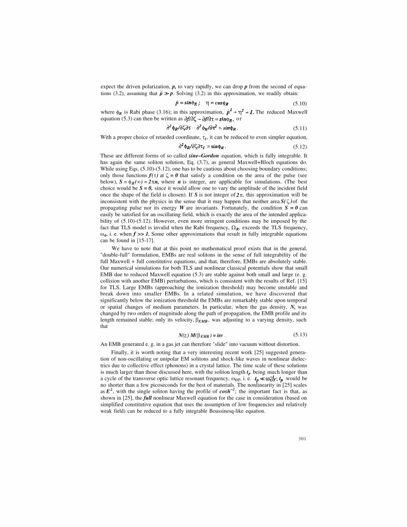
313

(10.13) resembles (10.9) with the main difference being that off-axis pulse stretches in time

by the factor Θ and its spectrum is respectively "squeezed" by the same factor.

Fig. 9. The evolution of the on-axis temporal profile (normalized field, Eon 0 vs normalized time, τ, and

the normalized amplitude spectrum, | S | 0 t0 , vs normalized frequency, v ≡ ωt0 (inset), of the initially

Gaussian half-cycle pulse, as it propagates along the axis Curves: 1, ζ = 0 ; 2, ζ = 0.25; 3,

ζ = 0.5; 4, ζ = 1; 5, ζ = 2 ; 6, ζ = 4. For the sake of comparison, each curve in the main Fig. is scaled up by

the factor w–1/2 (ζ).

In the so called low-frequency limit r0 << ct0 , opposite to (10.1), with the source size

being much smaller that the wavelength λ =2πc/ω of any frequency component, all the

components have the same dependence on the angle of propagation; also, the initial spatial

profile of the field becomes unimportant. The radiation pattern at each frequency is then

determined by an elementary (i. e. point-like) dipole formed by the field distribution,

(t,x,y). At the distance from this point-like source (i. e. away

from the very small near-field area ρnear << λ), and assuming that the field is linearlypolarized, the spectrum of radiative waves is:

(10.14)

where θ is now the angle between the axis z and the direction of propagation,

in the plane of the vector of polarization, and the observation point.

314

The Fourier transform of (10.14) produces the same time-derivative profile everywhere,

(10.15)

where is the polarization vector of radiative field, = cosθ. E q .

(10.15) explains pulse transformation in simple terms of elementary dipole antennae driven

by a current which is induced by the dynamics of one of the dipole electrical

"charges" q0 originated by the source field, E0 ; hence time-derivative temporal profile.Bearing in mind that for a Gaussian beam, Eq. (10.15) at θ=0 is consistent

with the Gaussian on-axis far-field (10.9), indicating that the results (10.6-10.12) for the

on–axis field are valid regardless of the condition (10.1). Furthermore, in far-field area,

Eq. (10.15) describes an on-axis field for any distribution, regardless of whether it is Gaus-

sian or not.

The dispersion and transformation of the pulse due to the propagation and diffraction

can to great degree be reversed. The feasibility of that is related to the time/space recipro-

city manifested here by Eq. (10.6) being invariant to the simultaneous sign reversal of time

τ and distance ζ. (The same is true for the solution (10.7), if E0 ( τ ) is a symmetric function,

see Eqs. (10.10)-(10.12).) In practice, the diffracted HCP can be transformed back almost

into its original temporal profile (except for its cw component) by reflecting its diffracted

wave front e. g. from a spherical concave mirror, if the angular aperture of the mirror is

significantly larger than the diffraction angle, θd . If such a mirror has the radius of curva-

ture Rm and is situated sufficiently far from the source, with the distance between them

being ƒ1 >> zd , the pulse is focused again into a tight spot at the distance ƒ2 , determined by astandard optical mirror formula, If ƒ2 <ƒ 1 , the area of this spot is smaller

that that of the original spot, and the amplitude of the focused pulse is larger by the factor

ƒ1 /ƒ2 . The residual distortion of the pulse (in particular, slight bipolarity of initially unipo-

lar HCP) will be due to lower-frequency diffraction losses at the mirror; the larger the mir-

ror size, the smaller this effect. In the case of point-like source, pulse restoration can be

achieved by using a full ellipsoid of revolution, with the source and observation points

situated at the foci of the ellipsoid.

11. CONCLUSION

In conclusion, we have theoretically demonstrated feasibility of powerful, near- and

sub-femtosecond sub-cycle EM pulses and solitary waves, EM bubbles, supported by both

quantum and classical nonlinear media. We have shown how their maximum amplitude

and minimum length are limited by the atomic ionization. It follows from our theory that

10 – 0.1 ƒs EMBs can be generated by the available half-cycle pulses and short laser pulses;

the peak EMB intensity can reach ~ 1014

– 1016 W/cm2. Those results represent only the

very first steps in the exploration of the new time domain. Our hope is that EMBs will be

experimentally observed in the near future. This will pose new set of problems, such as

EMB detection and characterization, separation, gating, control, focusing and guiding, and

exploring various EMB applications. In a transverse-limited EM field, a zero-frequency

spectral component of the incident HCP will not propagate beyond the near-field area, and

in the far-field area, EMB will assume a modified profile. Using analytic approach to the

diffraction-induced transformation of pulses with arbitrary temporal profiles, including

half-cycle pulses, we found close-form solutions for the propagation of most commonly

used initial spatio-temporal profiles, and explained the nature of time-derivative transfor-

mation in far-field area for arbitrary pulses.

315

The new time domain, being largely an uncharted territory, holds a lot of promises for

the physics of field-matter interaction. The most familiar nonlinear effects and parameters

associated with coherent light-matter interactions (harmonic generation, self-induced tran-

sparency, photon echoes, soliton generation and propagation, saturation of all kinds, n2 ,

χ (3) , etc.) are likely to take on entirely different forms, or may even cease to exist. One of

the most fundamental and intriguing phenomenon is the field ionization of atoms,

molecules, and semiconductor quantum wells by a super-short pulse with the amplitude

comparable to or larger than the ionization threshold. Such pulses could cause a substan-

tial "shake-up" excitation or ionization of an atomic system within the time much shorter

than any characteristic time of the system. In our most recent research [33] we showed that

a few ƒs long and unipolar EMB acting upon a semiconductor quantum well, can cause

both forward and backward field ionization, with the photoelectrons emitted in both direc-

tions (i. e. not only in the direction of the ionizing unipolar field) with comparable intensi-

ties. Even more fundamental and exciting results are obtained for the hydrogen atom hit

by a sub-cycle pulse with an sub-atomic unit amplitude. We also observed that the ioniza-

tion response of the atom consists of a sequence of well-separated peaks resulting in strong

spatio-temporal inhomogeneity of the photoelectron cloud, and found an explanation of

such a behavior.

This work is supported by AFOSR. The work by SFS is in part supported by the

Deutsche Forschungsgemeinschaft. AEK is a recipient of the Alexander von Humboldt

Award for Senior US Scientists of AvH Foundation of Germany.

REFERENCES

1.

2.

3.

4.

5.

6.

7.

8.

9.

10.

11.

12.

13.

316

S. L. McCall and E. L. Hahn, Phys. Rev. Lett. 18, 908 (1967).

P. W. Smith, Proc. IEEE, 1342 (1970) and references therein.

A. Hasegava and F. D. Tappert, Appl. Phys. Lett. 23, 142 (1971).

V. E. Zakharov and A. B. Shabat, Sov. Phys. JETP 34, 62 (1972).

(a) R. L. Fork, C. H. Brito Cruz, P. C. Becker, and C. V. Shank, Opt. Lett., 12, 483

(1987); (b) M. Nisoli, S. De Silvestri, O. Svelto, R. Szipocs, K. Ferencz, Ch. Spiel-

mann, S. Sartania, and F. Krausz, Opt. Lett. 22, 522 (1997).

K. E. Oughstun and H. Xiao, Phys. Rev. Lett. 78, 642 (1997); K. E. Oughstun and G.

C. Sherman, Electromagnetic pulse propagation in casual dielectrics (Springer,

Berlin, 1994).

P. R. Smith, D. H. Auston, and M. S. Nuss, IEEE JQE, 24, 255 (1988).

D. Grischkowsky, S. Keidin, M. van Exter, and Ch. Fattinger, JOSA B, 7, 2006

(1990); R. A. Cheville and D. Grischkowsky, Opt. Lett. 20, 1646 (1995).

J. H. Glownia, J. A. Misewich, and P. P. Sorokin, J. Chem. Phys. 92, 3335 (1990);

B. B. Hu and M. S. Nuss, Opt. Lett. 20, 1716 (1995);

R. R. Jones, D. You, and P. H. Bucksbaum, Phys. Rev. Lett. 70, 1236 (1993); C. O.

Reinhold, M. Melles, H. Shao, and J. Burgdorfer, J. Phys. B 26, L659 (1993).

A. E. Kaplan, Phys. Rev. Lett. 73, 1243 (1994); A. E. Kaplanand P. L. Shkolnikov,

JOSA B 13, 412 (1996).

A. E. Kaplan and P. L. Shkolnikov, Phys. Rev. Lett. 75, 2316 (1995); also in Int. J.

of Nonl. Opt. Phys. & Materials, 4, 831 (1995).

:

14.

15.

16.

17.

18.

19.

20.

21.

22.

23.

24.

25.

26.

27.

28.

29.

30.

31.

32.

33.

A. E. Kaplan, S. F. Straub and P. L. Shkolnikov, Opt. Lett., 22, 405 (1997); also to

appear in JOSA B 14 (1997).

R. K. Bullough and F. Ahmad, Phys. Rev. Lett. 27, 330 (1971); J. C. Eilbeck, J. D.

Gibbon, P. J. Caudrey, and R. K. Bullough, J. Phys. A 6, 1337 (1973).

E. M. Belenov, A. V. Nazarkin, and V. A. Ushchapovskii, Sov. Phys. JETP 73, 423

(1991).

A. I. Maimistov, Opt. & Spectroscopy, 76, 569 (1994) and 78, 435 (1995).

B. Kohler, V. Yakovlev, J. Ghe, M. Messina, K. R. Wilson, N. Schwentner, R. M.

Whitnell, and Y. Yan, Phys. Rev. Lett. 74, 3360 (1995)

A. E. Kaplan and P. L. Shkolnikov, Phys.Rev. A. 49, 1275 (1994).

For a harmonic oscillator with a frequency ω0 , it is natural to choose with

, where is the Compton wavelength.

If nonlinearity is negative, a < 0, one can expect formation of "dark" EMB (a solitary

"hole" propagating on a cw field background): ƒ(τ)∝ƒ0 tanh(τ ƒ0), ƒ 0 =const.

D. G. Lappas, M. V. Fedorov, and J. H. Eberly, Phys. Rev. A 47, 1327 ( 1993); J. H.

Eberly, Q. Su, and J. Javanainen, JOSA B 6, 1289 (1989).

Recent studies of shock-like envelope fronts can be found, e. g. in S. R. Hartmann

and J. T. Massanah, Opt. Lett. 16, 1349 (1991); E. Hudis and A. E. Kaplan, Opt.

Lett. 19, 616 (1994); W. Forysiak, R. G. Flesh, J. V. Moloney, and E. M. Wright,

Phys. Rev. Lett. 76, 3695 (1996).

R. M. Miura, J. of Math. Physics, 9, 1202 (1968); R. M. Miura , C. S. Gardner and

M. D. Kruskal, ibid, 1204 (1968); M. Wadati, J. Phys. Soc. Japan, 32, 1681 (1972);

ibid, 34, 1289 (1973)

L. Xu, D. H. Auston, and A. Hasegava, Phys. Rev. A45, 3184 (1992).

A. McPherson, G. Gibson, H. Jara, U. Johann, T. S. Luk, I. A. McIntyre, K. Boyer,

and C. K. Rhodes, JOSA B 4, 595 (1987); M. Ferray, A. L’Huillier, X. F. Li, L. A.

Lompre, G. Mainfray, and C. Manus, J. Phys. B 21, L31 (1988); A. L’Huillier and

Ph. Balcou, Phys. Rev. Lett. 70, 774 (1993); L’Huillier, A, Lompre, L. A., Mainfray,

G., and Manus, C., in Atoms Intense Laser Field , Ed. M. Gavrila (Acad. Press,

Inc., Boston, 1992), p. 139-206.

A. E. Kaplan, to appear in JOSA B.

Max Born and Emil Wolf, Principles of Optics, 6-th edition (Pergamon Press, NY,

1980).

A. Siegman, Lasers (Univ. Science, Mill Valley, CA, 1986); A. Yariv, QuantumElectronics (Wiley, NY, 1989).

M. van Exeter and D. R. Grischkowsky, IEEE Trans. Microwave Theory Techn., 38,

1684 (1990); J. Bromage, S. Radic, G. P. Agrawal, C. R. Stroud, Jr., P. M. Fauchet,

and R. Sobolevski, Opt. Lett. 22, 627 (1997).

R. W. Ziolkowski and J. B. Judkins, JOSA B 9, 2021 (1992).

I. S. Gradshtein and I. M. Ryzhik, Tables of Integrals, Series, and Products

(Academic, NY, 1980).

A. E. Kaplan, S. F. Straub and P. L. Shkolnikov, to be published; first reported in

Quant. Electr. & Laser Science Conf., v. 12, 1997 OSA Techn. Digest Series (OSA,

Washington, DC, 1997), p. 31.

317