Embed Size (px)
Citation preview

• Inventor of a “Bayesian analysis” for the binomial model
• Laplace at the same time discovered Bayes Theorem and a new analytic tool for approximating integrals
• Bayesian statistics was the method of statistics until about 1910.
Reverend Thomas Bayes 1702-1761
Mathematician who first used probability inductively and established a mathematical basis for probability inference He set down his findings on probability in "Essay Towards Solving a Problem in the Doctrine of Chances" (1763), published posthumously in the Philosophical Transactions of the Royal Society of London.

Statistics estimates unknown parameters (like the mean of a population).
Parameters represent things that are unknown. They are some propertiesof the population from which the data arise.
Questions of interest are expressed as questions on such parameters:confidence intervalls, hypothesis testing etc.
Classical (frequentist) statistics considers parameters as specific to the problem, so that they are not subject to random variability. Hence parametersare just unknown numbers, they are not random, and it is not possibleto make probabilistic statements about parameters (like the parameterhas 35% chances to be larger than 0.75).
Bayesian statistics considers parameters as unknown and random and henceit is allowed to make probabilistic statements about them (like the above).
In Bayesian statistics parameters are uncertain either because they are randomor because of our imperfect knowledge of them.

Example:
”Treatment 2 is more cost-effective than treatment 1 for a certain hospital.”
Parameters involved in this statement:- mean cost and mean efficacy for treatment 1- mean cost and mean efficacy for treatment 2
across all patients in the population for which the hospital is responsible.
Bayesian point of view: we are uncertain about the statement, hence thisuncertainty is described by a probability. We will exactly calculate the probability that treatment 2 is more cost-effective than treatment 1 for thehospital.
Classical point of view: either treatment 2 is more cost-effective or it is not.Since this experiment cannot be repeated (it happens only once), we cannot talk about its probability.

... but, in classical statistics we can make a test!
Null-hypothesis Ho: treatment 2 is NOT more cost-effective than treatment 1
... and we can obtain a p-value!
What is a p-value?

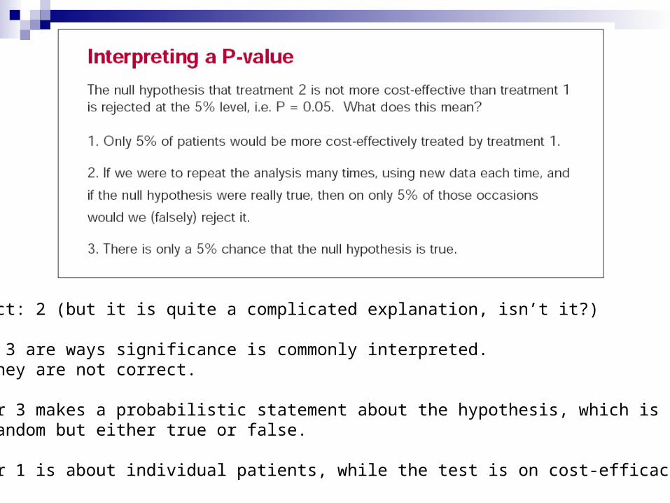
Correct: 2 (but it is quite a complicated explanation, isn’t it?)
1 and 3 are ways significance is commonly interpreted.BUT they are not correct.
Answer 3 makes a probabilistic statement about the hypothesis, which is not random but either true or false.
Answer 1 is about individual patients, while the test is on cost-efficacy.

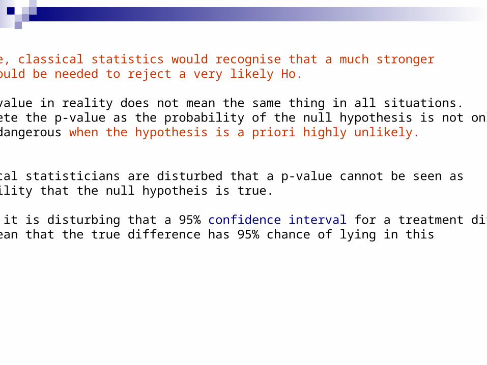
We cannot interprete a p-value as a probability, because in the classicalsetting it is irrelevant how probable the hypothesis was a priori, beforethe data where collected.
Example:
Can a healer cure cancer?A healer treated 52 cancer patients and 33 of these were better afterone session. Null Hypothesis Ho: the healer does not heal.p-value (one sided) = 3,5%. Hence reject at 5% level.
Should we believe that it is 96.5% sure that the healer heals?
Most doctors would regard healers as highly unreliable and in no waythey would be persuaded by a single small experiment. After seeing theexperiment, most doctors would continue to believe in Ho. The experimentwas due to chance.
In practice, classical statistics would recognise that a much stronger evidence would be needed to reject a very likely Ho.
So, the p-value in reality does not mean the same thing in all situations.To interprete the p-value as the probability of the null hypothesis is not onlywrong but dangerous when the hypothesis is a priori highly unlikely.
All practical statisticians are disturbed that a p-value cannot be seen asthe probability that the null hypotheis is true.
Similarly, it is disturbing that a 95% confidence interval for a treatment differencedoes NOT mean that the true difference has 95% chance of lying in this interval.
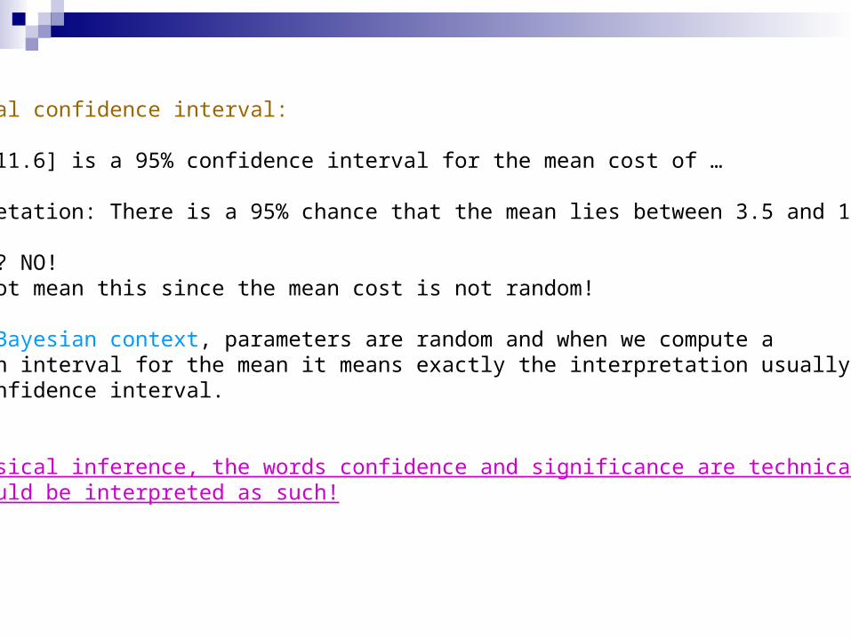
Classical confidence interval:
[3.5 – 11.6] is a 95% confidence interval for the mean cost of …
Interpretation: There is a 95% chance that the mean lies between 3.5 and 11.6.
Correct? NO!It cannot mean this since the mean cost is not random!
In the Bayesian context, parameters are random and when we compute aBayesian interval for the mean it means exactly the interpretation usually givento a confidence interval.
In classical inference, the words confidence and significance are technical termsand should be interpreted as such!

One widely used way of presenting a cost-effectiveness analysis is through the Cost-Effectiveness Acceptability Curve (CEAC),introduced by van Hout et al (1994). For each value of the threshold willingness to pay λ, the CEAC plots the probability that one treatment is more cost-effective than another. This probability can only be meaningful in a Bayesian framework. It refers to the probability of a one-off event (therelative cost-effectiveness of these two particular treatments is one-off, and not repeatable).
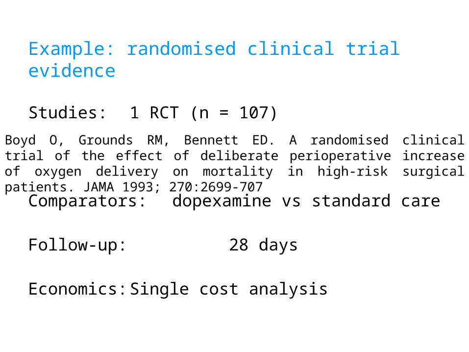
Example: randomised clinical trial evidence
Studies: 1 RCT (n = 107)
Comparators:dopexamine vs standard care
Follow-up: 28 days
Economics: Single cost analysis
Boyd O, Grounds RM, Bennett ED. A randomised clinical trial of the effect of deliberate perioperative increase of oxygen delivery on mortality in high-risk surgical patients. JAMA 1993; 270:2699-707

Trial results
Costs (£) Survival (days)mean se mean se
Standard 11,885£ 3,477£ 541 50.2Adrenaline 10,847£ 3,644£ 615 64.1Dopexamine 7,976£ 1,407£ 657 34.7

Trial CEAC curves
0
0.1
0.2
0.3
0.4
0.5
0.6
0.7
0.8
0.9
1
£0 £10,000 £20,000 £30,000 £40,000 £50,000 £60,000 £70,000 £80,000 £90,000 £100,000
Pro
bab
ility
str
ateg
y is
co
st-e
ffec
tive
Control Dopexamine Adrenaline

The Bayesian method: learn from the dataThe role of data is to add to our knowledge and so to update what we can sayabout hypothesis and parameters.
If we want to learn from a new data set, we have to first say what we alreadyknow about the hypothesis, a priori, before we see the data.
Bayesian statistics summerises the a priori known things on an unknown parameter(say the mean cost of something) in a distribution for the unknown quantity, calledprior distribution.
The prior distribution synthetises what is known or believed to be true before weanalyse the new data.
Then we will analyse the new data and summerise again the total informationabout the unknown hypothesis (or parameter) in a distribution called posterior distribution.
Bayes’ formula is the mathematical way to calculate the posterior distributiongiven the prior distribution and the data.

prior
data
posterior
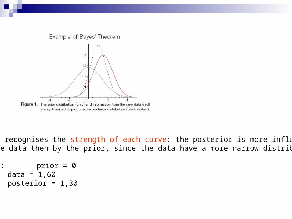
Bayes recognises the strength of each curve: the posterior is more influencedby the data then by the prior, since the data have a more narrow distribution.
Peaks: prior = 0data = 1,60posterior = 1,30
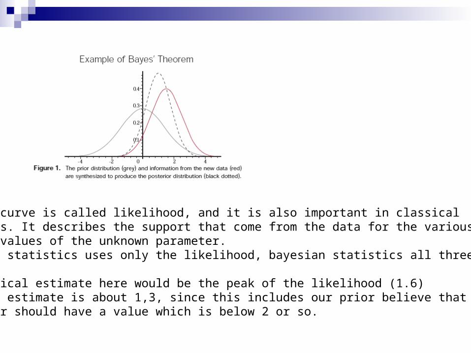
The data curve is called likelihood, and it is also important in classical statistics. It describes the support that come from the data for the variouspossible values of the unknown parameter.Classical statistics uses only the likelihood, bayesian statistics all three curves.
The classical estimate here would be the peak of the likelihood (1.6)The bayes estimate is about 1,3, since this includes our prior believe that thepartameter should have a value which is below 2 or so.

The bayesian estimate is a compromise between data and prior knowledge.In this sense, bayesian statistics is able to make use of moreinformation than classical statistics and obtain hence strongerresults.

Bayesian statistics reads confidence intervals, estimates etc from the posteriordistribution.
A point estimate for the parameter is the a-posteriori most likely value, the peakof the posterior, or the expected value of the posterior.
If we hav an hypothesis (for example that the paramter is positive), then we read from the posterior that the posterior probability for the paramter to belarger than zero is 0.89.
0.89

If we are less sure about the parameter a priori, then we would usea flatter prior. Consequence is that the posterior looks more similar tothe likelihood (data).

posterior = (constant number) prior likelihood prior likelihood
P(parameter | data) P(parameter) P(data | parameter)
P( | data) P() P(data | )
P( | data) = P() P(data | ) / P(data) (Bayes formula)

How do we choose a prior distribution?
The prior is subjective. Two different experts can have different knowledge and believes, which would lead to two different priors. If you have noopinion then it is possible to use a totally flat prior, which adds no informationto what is in the data.
If we want to have clear probabilistic interpretations of confidence and significance, then we need to have priors.
This is considered as a weakness by many who are trained to reject subjectivity whenever possible.
BUT:
- Science is not objective in any case. Why should the binomial or the gaussian distribution we the true ones for a data set?- subjective evidence can be tuned down as much as one wishes.- if there is no consensus, and different priors lead to different decisions, why hiding it?


Example: Cancer at Slater School(Example taken from an article by Paul Brodeur in the New Yorker in Dec. 1992.)
Slater School is an elementary school where the staff was concerned that their high cancer rate could be due to two nearby high voltage transmission lines.
Key Facts there were 8 cases of invasive cancer over a long time among 145 staff members whose average age was between 40 and 44 based on the national cancer rate among woman this age (approximately 3/100), the expected number of cancers is 4.2
Assumptions:1) the 145 staff members developed cancer independently of each other2) the chance of cancer, , was the same for each staff person.
Therefore, the number of cancers, X, follows a binomial distribution: X ~ bin (145, )
How well do each of four simplified Competing Theories explain the data?Theory A: = .03 (the national rate, i.e. no effect of lines)
Theory B: = .04Theory C: = .05Theory D: = .06

The Likelihood of Theories A-D
To compare the theories, we see how well each explains the data.
That is, for each hypothesized , we calculate the binomial distribution:
1378 )1(8
145 ) | 8 X Pr(
Theory A: Pr(X = 8 | = .03 ) .036
Theory B: Pr(X = 8 | = .04 ) .096
Theory C: Pr(X = 8 | = .05 ) .134
Theory D: Pr(X = 8 | = .06 ) .136
This is a ratio of approximately 1:3:4:4. So, Theory B explains the data about 3 times as well as theory A. There seems to be an effect of the lines!

A Bayesian Analysis There are other sources of information about whether cancer can be
induced by proximity to high-voltage transmission lines.- Some epidemiologists show positive correlations between cancer and proximity- Other epidemiologists don’t show these correlations, and physicists and biologists maintain believe that energy in magnetic fields associated with high-voltage power lines is too small to have an appreciable biological effect.
Supposes we judge the opposite expert knowledge equally reliable. Therefore, Theory A (no effect) is as likely as Theories B, C, and D together, and we judge theories B, C, and D to be equally likely. So, Pr(A) 0.5 Pr(B) + Pr(C) + Pr(D)Also, Pr(B) Pr(C) Pr(D) 0.5 / 3 = 1/6
These quantities will represent our prior distribution on the four possible hypothesis.
prior

Bayes’ Theorem
23.0)8|Pr(
)136)(.6/1()134)(.6/1()096)(.6/1()036)(.2/1(
)036)(.2/1()8|Pr(
)D|8 Pr(X D)Pr()C|8 Pr(X C)Pr()B|8 Pr(X B)Pr()A|8 Pr(X A)Pr(
)A|8 Pr(X A)Pr()8|Pr(
8) Pr(X
)8 X andA Pr()8|Pr(
XA
XA
XA
XA
P( A | X = 8 ) = 0.23
Likewise,
Pr( B | X = 8 ) = 0.21
Pr( C | X = 8 ) = 0.28
Pr( D | X = 8 ) = 0.28
Accordingly, we’d say that each of these four theories is almost equally likely,
So the probability that there is an effect of the lines at Slater is about
0.21 + 0.28 + 0.28 = 0.77. So the probability of an effect is pretty high, but not close enough to 1 to be a proof.
posterior

A non-Bayesian Analysis Classical test of the hypothesis
Ho: = .03 (no effect)
against the alternative hypothesis.
Calculate the p-value; we find:
p-value = Pr(X=8| = 0.03 )+ Pr(X=9| = 0.03 )+ Pr(X=10| = 0.03 )
+…+ Pr(X=145| = 0.03 ) (138 terms to be added)
.07
Under a classical hypothesis test, we would not reject the null hypothesis. So there is no indication of an effect of the lines.
By comparison, the Bayesian analysis revealed that the probability that Pr( > .03) 0.77

Today’s posterior is the prior of tomorrow!

Example: Hospitalisation
A new drug seems to have good efficacy relative to a standard treatment.Is it cost-effective? Assume that it would be so if it would also reduce hospitalisation.
Data: 100 patients in each treatment group. Standard treatment group: 25 days. (sample variance was 1.2)New treatment group: 5 days. (sample variance was 0.248)
Classical test (do it!) would show that the difference is significant at 5% level.Pharmaceutical company would then say: ”The mean number of days inhospital under the new treatment is 0.05 per patient (5/100) while it is 0.25with the standard treatment.” Cost effective!!!!!

Example: Hospitalisation & genuine prior information
BUT: this was a rather small trial.Is there other evidence available?
Suppose a much larger trial of a similar drug produced a mean numberof days in hospital per patient of 0.21, with a standard error of 0.03 only.
This would suggest that the 0.05 of the new drug is optimistic and thereis a doubt on the real difference between new and standard treatment cost.
BUT, the interpretation of how pertinent this evidence is, is subjective. It wasa similar, not the same drug.
It is however reasonable to suppose that the new drug and this similar one should be rather similar.
Because the drug is not the same, we cannot simply put the two data setstogether. Classical statistics does not know what to do, except to lower the required significance.
Example: Hospitalisation
Bayesian statistics solves the problem by treating the early trial as giving prior information to the new trial.
Assume that our prior says that the mean number of days inhospital per patient with the new treatment should be 0.21 but with a standard deviation which is larger, say 0.08, to mark that the twodrugs are not the same.
Now we compute the posterior estimate, given the new small trial,and obtain that the number of days in hospital per patient is 0.095.
So this is still better than the standard treatment (0.25 days). In fact we can compute the probability that the new drug reduces hospitalisation with respect to the standard one and we get 0.90!
Conlcusion: the new treatment has a 90% chance to reduce hospitalisation(but not 95%) and that the mean number of days is about 0.1 (not 0.05).

http://www.bayesian-initiative.com/
The Bayesian Initiative in Health Economics & Outcomes Research

I hope I have not confused you too much!
BUT I also hope that you are a bit confused now and that at later stagesin your education and profession you will want to learn this better!
For now: Bayesian statistics is NOT part of the pensum.