9/23/12

1

Bayesian Statistics Applied to Reliability Analysis and Prediction

By Allan T. Mense, Ph.D., PE, CRE,

Principal Engineering Fellow,

Raytheon Missile Systems, Tucson, AZ

1. Introductory Remarks.

Statistics has always been a subject that has baffled many people both technical and non technical. Its

basis goes back to the mid 18th century and the analysis of games of chance. Statistics is the application

of probability and probability theory can be traced to the ancient Greeks but it was most notably

developed in the mid 17th century by the French mathematicians Fermat, Laplace, and others. Rev. Sir

Thomas Bayes (born London 1701, died 1761, see drawing below) had his works that includes the

Theorem named after him read into the British Royal Society proceedings (posthumously) by a colleague

in 1763. I have actually seen the original publication!

For years and even in the present day the statistics

community seems to have a schism between the so-called

“objectivists or frequentists” and their so-called “classical”

interpretation of probability and the Bayesians who have a

broader interpretation of probability. From a reliability point

of view classical calculations can be thought of as a subset of

Bayesian calculations. You do not have to give up the

classical answers but you will have to give up the classical

interpretation of the results!

Discussion of the logical consistencies and inconsistencies of

the two statistical points of view would lead us too far afield

[5] . However my personal observations indicate that in the

battle over which techniques to apply to problems, the Bayesian have won the war but classical

techniques are still widely used, easy to implement and are very useful. We will use both but the

purpose of this note is to explain Bayesian techniques applied to reliability.

References. The two major texts in this area are “Bayesian Reliability Analysis,” by Martz & Waller [2] which is out of print and more recently “Bayesian Reliability,” by Hamada, Wilson, Reese and Martz [3]. It is worth noting that much of this early work at Los Alamos was done on weapon system reliability and all the above authors work or have worked at the Los Alamos National Lab [1]. Allyson Wilson headed the Bayesian reliability group at LANL and Christine Anderson-Cook now heads that group. They are arguably among the leading authorities in Bayesian reliability in the world. I will borrow freely from both these texts and from notes I have from their lectures. There are also chapters covering Bayesian

9/23/12

2

methods in traditional reliability texts e.g. “Statistical Methods for Reliability Data,” Chapter 14, by Meeker and Escobar [4]. This point paper covers Bayesian reliability theory and Markov Chain Monte Carlo (MCMC) solution methods. The NIST web site also covers Bayesian reliability. Specifically 8.2.5. covers “What models and assumptions are typically made when Bayesian methods are used for reliability evaluation?”

Philosophy.

The first and foremost point to recognize is that reliability has uncertainty and therefore should not be

thought of as a single fixed number whose unknown value we are trying to estimate. Reliability having

this uncertainty requires us to treat reliability as a random variable and therefore discuss it using

probability distributions, f(R), and the language of statistics i.e. how likely is it that reliability of a system

or component will have some value greater than some given number (typically a reliability specification).

We will see that specifying some desired reliability value is not sufficient but requires that we also specify

some level of confidence that reliability is greater than (or less then) the value desired. This will become

clear when reliability distributions are defined and calculated.

For those needing a refresher on statistics I recommend “Introduction to Engineering Statistics,” by

Doug Montgomery et al

and any edition of this

text will do just fine. The

fundamental concepts

you will need are 1)

probability density

functions, pdf, written as

f(x|a,b,c) where the

letters a,b,c refer to

pieces of information,

called parameters, that

are presumed known,

knowable or can be

estimated , 2) cumulative

distribution function

(CDF), written F(x|a,b,c),

which is the accumulated

probability of the

random variable X from the minimum allowable value of X (typically zero or -∞) up to X=x, and 3) the

concept of a likelihood function which in practice is the product of pdf’s and CDF’s evaluated in terms of

all the available data.(See Appendix G ). The use of a likelihood function while familiar to every

statistician is not used by everyday reliability engineers! The concept was proposed by Sir Ronald Fisher

back in the early 1900’s and is very useful.

For those not familiar with the traditional “frequentist” method for establishing a reliability estimate

and its confidence interval, Appendix C has been provided.

Why Bayesian

• Bayesian methods make use of well known, statistically

accurate, and logically sensible techniques to combine different

types of data, test modes, and flight phases.

• Bayesian results include all possible usable information base

on data and expert opinion.

• Results apply to any missile selected and not just for “average

sets of missiles”.

• Bayesian methods are widely accepted and have a long track

record:

FAA/USAF in estimating probability of success of launch vehicles

Delphi Automotive for new fuel injection systems

Science-based Stockpile Stewardship program at LANL for nuclear

warheads

Army for estimating reliability of new anti-aircraft systems

FDA for approval of new medical devices and pharmaceuticals

9/23/12

3

It is also worthy of note that Bayesian reliability has been actively pursued for at least 30 to 40 years and

the Los Alamos National Lab (LANL) developed the techniques to predict the reliability of missiles as well

as the nation’s nuclear stockpile back in the 1980’s and before.. The reasons for using Bayesian can be

summarized and are outlined in the chart shown on the previous page.

Before proceeding in detail there is a simple picture to keep in mind that explains how Bayesian

reliability analyses works. One starts by (1) producing the “blue” curve (prior distribution) based upon

previous information deemed useful for predicting the probability of successfully operating units prior to

taking data on the system or component of interest, then (2) folding in recent test data as is represented

by the “red” distribution (likelihood function) and finally (3) producing, using some rather sophisticated

math in the general case, a curve such as shown in “green” in Figure 4. The green curve represents the

posterior distribution of a unit’s reliability given the most recent data. From this green curve we can in

principle, calculate everything that is needed.

Figure 7. The Prior, Likelihood and Posterior, superimposed. One postulates from previous information a prior

distribution shown in blue. The tests are performed and put into a likelihood function shown graphically in red. The

result (in green) is the answer. It is the posterior reliability distribution.

Note that the posterior distribution (green) is more peaked and narrower than the (red) likelihood curve

which is indicative of having prior information on the reliability. The likelihood function (red) by itself

would be the distribution found from classical or frequentist analysis i.e. from a prior that is uniform.

9

Posterior Distribution combining

Prior and Data

• Blue curve is our prior distribution

• Red curve is distribution assuming only information is 4 successes in 5 tests

• Green curve is the Bayesian estimate adding the 4 out of 5 to the prior

– Estimate is between evidence (data) and prior

– Distribution is tighter than prior or data only narrower confidence bounds

0 0.1 0.2 0.3 0.4 0.5 0.6 0.7 0.8 0.9 1

System Reliability

Pro

babi

lity

Den

sity

Fun

ctio

n

Posterior distribution of

System Reliabilityafter 4

successes in 5 tests

Initial distribution of

System Reliability

assuming the most

probable value is 0.90

Likelihood of System Reliability

using 4 successes in 5 tests only

9/23/12

4

Finding the (green) posterior distribution for real situations is mathematically complex, but the essence

of what is done is as simple as the graphical display shown above. For those caring to delve further in

the details, the following sections have been provided.

Table of Contents.

Introductory remarks

References

Philosophy

Overview

Basic Principles

Bayes’ Theorem: Prior, Likelihood, Posterior

Bayes’ Theorem Allied to Pass/Fail Reliability

General Bayesian Approach to Reliability

General Procedure for Bayesian Analysis and Updating

Selecting a Prior

Likelihood Function

Generating System Level Reliability Estimate

Summary

Time Dependent Reliability Calculations Using a Weibull Distribution

Poisson Counting

Appendices

2. Overview

It makes a great deal of practical sense to use all the information available, old and/or new, objective or

subjective, when making decisions under uncertainty which is exactly the situation one has with many

systems in the field. This is especially true when the consequences of the decisions can have a

significant impact, financial or otherwise. Most of us make everyday personal decisions this way, using

an intuitive process based on our experience and subjective judgments.[6]

Using language from the NIST web site we note that so-called classical or frequentist statistical analysis, seeks objectivity by generally restricting the information used in an analysis to that obtained from a current set of clearly relevant data. Prior knowledge is not used except to suggest the choice of a particular population model to "fit" to the data, and this choice is later checked against the data for reasonableness. What is wrong with this approach after all it has used successfully for many years? The answer lies in the desire to take into account previous information particularly if we have some information from flight tests and some from ground tests and we want to somehow combine this information to predict future probabilities of success in operational scenarios. For example why throw away knowledge gained in lab tests or ground tests even though the testing environments do not duplicate the flight operational environment. We use Bayesian statistics and the only known (to this author) way to incorporate this knowledge quantitatively into reliability calculations. The use of Bayesian statistics makes use of this prior information and should lead to savings of time and money while providing “useable” information to the product engineer.

9/23/12

5

classical Bayesian

R, fixed R, random

estimate distribution

<R>=s/n f(R )

s=# successes Pr{R>r}

n=# tests 1-F(R )

useage usage

P(k successes|m future tests,<R>) P(k successes|m future tests)

{ | , } (1 )k m km

P k m R R Rk

0

{ | } (1 ) ( )k m k

R

mP k m R R f R dR

k

Lifetime or repair models using frequentist methods have one or more unknown parameters. The frequentist approach considers these parameters as fixed but unknown constants to be estimated using sample data taken randomly from the population of interest. A confidence interval for an unknown parameter is really a frequency statement about the likelihood that numbers calculated from a sample capture the true parameter, e.g. MTBF. Strictly speaking, one cannot make probability statements about the true parameter since it is fixed, not random. It is the interval that is random and once you take data and calculate a confidence interval then either the reliability is in the calculated interval or it is not.

The Bayesian approach treats these population model parameters as random, not fixed, quantities. Before looking at the current data, use is made of old information, or even subjective judgments, to construct a prior distribution model for these parameters. This model expresses the starting assessment about how likely various values of the unknown parameters are. Then use is made of the current data (via Bayes’ formula) to revise this starting assessment, deriving what is called the posterior probability distribution model for the population model parameters. Parameter estimates, along with confidence intervals ---known as credibility intervals in Bayesian vernacular----, are calculated directly from the posterior distribution. Credibility intervals are legitimate probability statements about the unknown parameters, since these parameters now are considered random, not fixed.

In the past parametric Bayesian models were chosen because of their flexibility and mathematical convenience [1,2]. The Bayesian approach is performed in Raytheon codes (RBRT1 and RBRT2. The Los Alamos National Laboratory (LANL) has also developed and is marketing their Bayesian Code called SRFYDO.

A comparison is shown below between classical (frequentist) approach and the Bayesian approach. The key to Bayesian is the process of determining f(R ), the posterior distribution (probability density function).

9/23/12

6

0

0.5

1

1.5

2

2.5

3

3.5

4

4.5

5

0 0.1 0.2 0.3 0.4 0.5 0.6 0.7 0.8 0.9 1

f(R

), p

df

R, Reliability

Bayesian Reliability

Prior

Likelihood

Posterior

A typical (posterior)

distribution for f(R )

is shown in the graph

below in green.

How one arrives at

this distribution is

discussed in great

detail later. The

green curve

represents the f(R)

we are seeking.

Again I note the

distribution is not an

end in itself. One

uses f(R) to 1)

predict the credibility

interval for reliability

and 2) when

multiplied times the binomial distribution (for example) and integrated over all possible values of R gives

the answer to the question of what is the probability of any given number of successes in some future set

of tests. See Bayesian Calculator Rev5.xls. The rest of this white paper concentrates on calculational

procedures and some insightful examples of Bayesian reliability analysis.

3. Basic Principles

Bayes’ analysis begins by assigning an initial distribution of possible unit reliabilities (fprior(R)) on the basis

of whatever evidence is currently available. The initial predictions may be based 1) solely on engineering

judgment, 2) on MIL HDBK 217, 3) on data from other techniques such as simulation, or 4) combinations

of all of the above. Initial reliabilities are known as prior reliabilities because they are determined

BEFORE we run our experiments on the system of interest. When necessary, these priors can be

determined for each and every component within the overall system or more appropriately we may

decide to specify a prior only at the system or subsystem level. If one assumes the reliability of each

component is equally likely to have a value between R=0 to R=1 (not a smart assumption in most cases),

then one is de facto performing the equivalent of the classical of frequentist analyses but the

interpretation of the results is entirely different. Thus classical results are reproducible from Bayesian

analysis. The converse is not true.

All reliability analyses must obey Bayes’ theorem. By explicitly stating the assumptions for prior

distributions one can convincingly show how reliability distributions (probabilities) evolve as more

information becomes available. Examples will be shown later in this note.

Digression: In addition there is a subtlety in the interpretation of Bayesian analyses that gives it a more

useful interpretation than does the classical or frequentist analyses. I know this sounds vague but it

needs to be discussed later when one is more familiar with the Bayes’ formalism.

The prior reliabilities are assigned in the form of a distribution and determined before the acquisition of

the additional data. In general, a prior distribution must be determined with some reasonable care as it

9/23/12

7

will play a major role in determining the reliability distribution of the system until there is sufficient data

to outweigh the prior distribution.

Think of the prior as a statement of the Null Hypothesis in classical hypothesis testing – it is the status

quo or what we already know. In statistical terminology we are testing (comparing in a sense) the

result, called the posterior distribution, to our Null Hypothesis, called the prior distribution which is

based upon knowledge previously acquired about the product whose reliability we are questioning.

For example, if we know the reliability of a unit is certainly > 50% and probably less than say 99% then

we might use a uniform distribution between 0.5 and 0.99 with the probability being zero elsewhere as

a useful prior. This would be one of many acceptable but not very useful priors.

The question is which of this infinite set of choices for a prior should be used in the analysis process.

Some of this answer comes from the literature from which many analyses have been performed with

various priors. Some of the answer comes from noting that expert opinion is valid and the prior is a

quantitative way to capture this opinion or experience. For reliability work we choose priors that give

the data “room to move” yet emphasize the regions of R values that characterize or history based on

prior knowledge. This is always a qualitative trade off and different SME’s will have different opinions.

The practicing Bayesian reliability engineer must assess these expert opinions and perform some

tradeoffs. In my experience reliability analysis Bayesian style is NOT a “cookbook” approach and

requires some consensus building.

As will be seen shortly the exact form of the prior 1) matters little once a reasonable amount of data is

collected from the system of interest but 2) does carry some importance when there is only a small

amount of test data. The prior (being non uniform in most Bayesian approaches) keeps the reliability

prediction based on operational data from being either too optimistic or too pessimistic. Consider the

following: you run one test and it is a success would you predict, based on one data value, that the

entire population of uints has a reliability of 1? Similarly if the single unit test failed would you tell the

customer that the predicted reliability of all the units built is 0? I doubt that either conclusion would be

acceptable but how do you know and more importantly what can you say about it? Well, we have expert

knowledge from having built systems of similar complexity in the past. When these previous units went

into full production the fraction of successful tests of the units in the field has almost always > 80% and

many times much higher. So as experts we want to take advantage of that knowledge and experience

and the method of doing this in a quantitative manner is by applying Bayesian statistics.

Given the priors, tests are performed on many systems. The data from these tests is entered into what is

called a likelihood function, e.g. ( | , ) (1 ) ( 1, 1)s n sL R s n R R B s n s where n=# tests, s=#

successes. Note: The likelihood function treats R as a random variable and the test data (n,s) as known

as opposed to a binomial distribution that treats R as known and predicts s. Likelihood functions are

discussed in Appendix F.

There is a likelihood function for every component in the unit’s system, every subsystem, and the unit as

a whole. If Bayesian methods are not used, then this likelihood function is the starting point for classical

9/23/12

8

reliability analysis. This is equivalent from a mathematical viewpoint to having used a uniform prior that

ranges from 0 to 1, i.e. we are ignorant as to the range of reliabilities the unit might have. When you

think about it for a moment it seems clear that assuming we know nothing about reliability of the

products we build is cause for not selecting us to build any units! Uniform in a Bayesian reliability

context is analogous to saying you are lacking in experience.

The product of the prior reliability distribution times the likelihood function results in what is known as a

joint reliability distribution. From this joint distribution one can form a posterior reliability distribution

(fposterior(R)). It is this posterior distribution that we seek to find. It gives the analyst a better picture of the

system reliability and its variability.

In short, the advantage in using Bayesian statistics is that it allows prior information (e.g., predictions,

test results, engineering judgment) to be combined with more recent information, such as test or field

data, in order to arrive at a prediction/assessment of reliability based upon a combination of all available

information and provided in the form of a probability distribution that can be used for further important

assessments.

As will be seen, Bayesian statistics is particularly useful for assessing the reliability of systems where only

limited field data exists. It can also handle correlated failure modes where for example partial failures or

degradation of some components can affect one another and cause subsystem and system failures

when component failures are not recorded.

In summary, It is important to realize that early test results do not tell the whole story. A reliability

assessment comes not only from testing the product itself, but is affected by information which is

available prior to the start of the test, from component and subassembly tests, previous tests on the

product, and even intuition based upon experience, e.g. comprehensive reliability tests may have been

performed on selected subsystems or components which yield very accurate prior information on the

reliability of that subsystem or component. Why should this prior information not be used to supplement

the formal system test result? One needs a logical and mathematically sound method for combining this

information. Besides one can save as much as 30% to 50% in testing for the same level of confidence and

that means savings in time, resources and money.

One of the basic differences between Bayesian and non-Bayesian (frequentist) approaches is that the

former uses both current data and prior information, whereas the latter uses current data only.

To see how all this discussion is turned into quantitative and useful information one begins with a basic

understanding of Bayes’ Theorem.

4. Bayes' Theorem

One of the axioms of probability theory states that the probability that two events, A and B, occur is

equal to the probability that one occurs, labeled P(A), multiplied by the conditional probability that the

other occurs, given that the first occurred, labeled P(B|A).

Written as a formula:

9/23/12

9

P(A and B) = P(A)P(B|A) =P(AB) (1)

The symbol is called an “intersection.” One notes that it makes no difference if one interchanges A

with B since the calculation is the probability they both occur. There need not be time ordering of the

events. Thus, the following expression must also be true.

P(B and A) = P(B)P(A|B) =P(BA) (2)

Setting equations (1) and (2) equal to one another, it follows directly that

P(B)P(A|B) = P(A)P(B|A).

Solving these two terms for P(A|B), one arrives at Bayes’ Theoremi.

P(A|B) = [P(B|A) / P(B)] P(A) (Bayes’ Theorem) (3)

Posterior = [Relative Likelihood] X Prior

The terms in the square brackets is called the relative likelihood. The probability P(A) is called the prior

probability and P(A|B) is called the posterior probability, it is the conditional probability of event A

occurring given information about event B. The addition of information, e.g. event B occurring, affects

the probability of A occurring. The information changes the probability from P(A) to P(A|B). If

information did not change the probability of detection we would be out of the sensor business. The

areas of recognition, detecting signals in the presence of noise, and implementing Kalman filters

requires Bayesian thinking and calculational framework.

This above extremely simple result holds a great deal of powerful logic. As a mathematical theorem it is

always true given the assumptions leading to the theorem are true. The requirement is simply that one

is dealing with random processes that have measurable probabilities. This is so very broad one is hard

pressed to find situations in which the theorem does not apply.

In the following material you will be lead through Bayesian reliability analysis when there is only

pass/fail or binary data. This will be followed by some discussion about how to solve Bayesian reliability

problems when one has causal variables that affect the reliability e.g. age of the unit, exposure to high

humidity, etc. This is the situation for which the RMS tool, RBRT2, was developed. This material will then

be followed by a time-dependent reliability problem. Typically this time dependent analysis involves

exponential, Weibull, lognormal or other distributions and even includes Poisson distributions when the

interest is in counting the number of failures over a given span of time.

5. Bayes’ Theorem Applied to Reliability as measured by Pass/Fail tests.

The idea that reliability is some single number is not a good way to think about reliability because

reliability has randomness i.e. there is a lot of variability or uncertainty involved in determining reliability

particularly for a complex system and even more variability with a collection of such systems. To account

for this uncertainty one must assign probabilities for a range of possible reliabilities. This is most

9/23/12

10

conveniently done using what is called a probability density function (pdf) or sometimes simply the

reliability distribution, f(R). Figure 1 below is an example of such a distribution (shown in blue).

Figure 1. Probability Density Function. Blue curve on graph shows the relative probabilities of occurrence of a

range of possible reliabilities. Mean reliability, E[R]=0.892 and the most probable reliability (peak of curve; the mode)

occurs for R = 0.9.

To use this chart quantitatively one must be able to find the area under the curve. For example, the

area under curve to the right of 0.9 indicates the probability (confidence) of having a reliability greater

than 0.9. This may sound abstract but it is the manner one must address reliability to be correct.

Say that this particular pdf represents the reliability of units in the lot [1]. The peak of this graph gives

the most probable reliability (called the mode). If a unit is randomly picked from a lot, the reliability of

the unit is likely to be close to this most probable value. But there are many unitss that may be more

reliable and many that may be less reliable. The probability that a randomly picked unit has reliability

greater than the most probable value is easily found using the cumulative probability distribution (CDF)

function, shown below in Figure 2.

Reliability Distributions

0

2

4

6

8

10

12

14

16

18

20

0.5 0.55 0.6 0.65 0.7 0.75 0.8 0.85 0.9 0.95 1

R, reliability

f(R

), p

df

0

0.1

0.2

0.3

0.4

0.5

0.6

0.7

0.8

0.9

1

Pr{

Reliab

ilit

y >

R}

f(R ) 1-F(R )

Probability that

reliability > 0.9 is

given by shaded

region and read

from cumulative

curve to be ~ 0.42

9/23/12

11

Figure 2. The Cumulative Distribution Function, F(R), for the reliability. Each value F(R) represents the area

under the f(R) curve (Figure 1) from zero up to the reliability value R. The probability that a unit has a reliability below

any given value of R can be read directly from the vertical scale; F(R) = P(reliability < R); e.g., P(reliability < 0.9) =

58%. Obviously the probability the reliability is greater than R equals 1 – F(R ).

Noting from Figure 1 that the most probable value of R is 0.9, the corresponding value for F(R=0.9) =

0.58, which is the probability that reliability is less than 0.9. So the probability {choosing a unit with a

reliability greater than 0.9} is simply 1 - 0.58 = 0.42, signifying that there is a 42% probability of

randomly choosing a unit from the lot with a reliability greater than 0.9. Restated we would say that we

are 42% confident that the reliability of the next unit chosen (at random) from the lot of many units in

the field has a reliability of 90% or greater.

Understanding these graphs is essential to understanding reliability. Once these curves are produced,

their interpretation is relatively straightforward.

6. General Bayesian Approach to Reliability

All of Bayesian reliability is explained by the following simple formula.

(( |( | ) ) )priorposteriorf LR data ta fda R R (4)

Equation (4) is Bayes’ Theorem for reliability distributions. In words, the posterior distribution for

reliability given the evidence (new data), equals the product of the prior information (distribution) and

the new data, formulated as a Likelihood Function and this product is then normalized so it integral over

all reliability values = 1. The complications occur when we have many components and many possible

Pr{reliability <R}

0

0.1

0.2

0.3

0.4

0.5

0.6

0.7

0.8

0.9

1

0.7 0.75 0.8 0.85 0.9 0.95 1

R, reliability

F(R

), C

DF

9/23/12

12

0

0.2

0.4

0.6

0.8

1

1.2

0 0.2 0.4 0.6 0.8 1

Like

liho

od

(n,s

|R)

R

Likelihood n=s=1

factors that may influence the components operation. We will attempt to add in the complications a

small amount at a time.

Given the formula above the actual mechanics of applying Bayesian probability to reliability distributions

is very straightforward.

1. One constructs from previous experience and expert knowledge a probability function called a prior distribution to represent the relative probabilities predicted prior to testing the units, i.e. construct fprior(R). This is similar to knowing P(A) in equation (3) but now a distribution of possible reliability values is provided, instead of a single value.

Figure 3, A Prior Distribution example using a beta distribution.

2. Tests are performed and that test data is put into a likelihood function, L(data|R), similar to the [P(B|A) / P(B)] term in equation (3). The likelihood function, L(data|R), will be discussed below as it carries all recent test information.

Shown below is the Likelihood function for the case where there was 1 test (n=1) and it resulted in a success (s=1). By the way this is the only function you would see in a classical reliability analysis. Most reliability engineers are not used to seeing the binomial reliability graphed in this form because the binomial probability treats the

number of successes (s) as the random variable and assumes R is known (or well estimated). In the likelihood function we treat s and n as known and ask what is the probability (likelihood) of achieving these experimental results for different values of R?

Figure 4. The likelihood function for the case of one test that results in a success.

0

0.01

0.02

0.03

0.04

0.05

0.06

0.07

0.08

0.09

0 0.2 0.4 0.6 0.8 1

f(R

,pri

or

), p

df

R

fprior(R )

9/23/12

13

00.002

0.004

0.006

0.008

0.01

0.012

0.014

0.016

0.018

0.02

0 0.2 0.4 0.6 0.8 1

f(R

,po

ste

rio

r),p

df

R

Posterior

3. Finally Bayes theorem is used to find the posterior reliability distribution, fposterior(R|data), that is conditioned (depends upon) by the actual data and weighted in some sense by the prior predictions assumed before the testing. This requires taking the product of the prior distribution and the likelihood function for all subsystems in the unit. The result is an equation of the form shown previously as equation (4) and illustrated below. The formulas are simple examples.

Figure 5. The posterior distribution.

Many times it is convenient to show both the posterior pdf, f(R ) and the so-called survival function

S(R)=1-F(R) that gives the Pr{reliability >R}. This is shown below.

Figure 6. combined look at both f(R) and S(R)=1-F(R).

Note: The prior and posterior distributions in equation (4) do not have to be of the same functional form

(i.e., conjugates). .

0

0.2

0.4

0.6

0.8

1

0

0.005

0.01

0.015

0.02

0 0.2 0.4 0.6 0.8 1

Pr{

relia

bili

ty >

R}

f(R

,po

ste

rio

r), p

df

R

Posterior pdf and Pr{reliability >R}

Posterior S(R )

(1 )

, arg

(1 )( | , , , )

( 1, (1 ) 1)

m mN s N n s

posterior

m m

s n l em

m

R Rf R n s Nm

B N s N n s

N s sMode

N n n

(1 )(1 )

( | , )( 1, (1 ) 1)

m mN N

m m

R Rf R Nm

B N N

(1 )( | , )

( 1, 1)

s n sR Rf R n s

B s n s

sMode

n

9/23/12

14

7. General Procedure for Bayesian Analysis and Updating The Raytheon Bayesian reliability tool RBRT-2 performs Bayesian reliability analyses on complex systems

whose functional components are assumed to all be in series from a reliability standpoint, i.e. if any

single component fails the system fails. It also just works with Pass/Fail or what we call binary data.

A demonstration of how this tool works will be performed at the end of this white paper for a simple

case of three components in series.

The initial prior assessment is represented by a probability distribution with certain parameters. The

prior distribution is updated using the evidence, resulting in a posterior distribution with its own

parameters. Statistical inferences can then be made from information conveyed by the posterior

distribution.

1. Select an appropriate prior probability distribution 2. Obtain new evidence (data) 3. Choose a likelihood function, based on the data type 4. Update the prior distribution with the new evidence to generate a posterior probability

distribution 5. Use the most recent posterior distribution as the new prior 6. Re-iterate steps 2 through 5.

8. Selecting the Prior Since prior knowledge exists for the reliability of each subsystem, we can use a prior distribution that

takes our existing knowledge into account. As an example if we were to select a beta distribution as a

prior for each subsystem we would have a lot of flexibility to match previous data and account for

expert analyses. Such a distribution was shown in Figure 3 as the blue curve. The names are not

important the shape of the distribution is important and that is why one uses functional forms for the

prior that can represent many possible shapes. One can specify the prior distribution as a series of

numerical values if necessary to more accurately reflect previous knowledge or one can perform what is

called Gaussian kernel smoothing techniques on discrete distribution values taken from data. There is

no requirement to use some type of “named” probability distribution.

The initial prior distribution represents the user’s prior beliefs and confidence about the reliability or

unreliability of the items. Prior distributions range from “weak” to “strong”. Weak distributions are

wide and relatively flat, and have less influence on the analysis, (the uniform distribution with f(R) = 1

for (0<R<1) has no influence) but its use will require more data (test evidence) to achieve a desired

accuracy for the posterior distribution. Strong distributions are narrow and peaked, indicating a strong

belief and high confidence in the region over which significant reliability exists.

The more accurate the prior, the quicker the analysis will arrive at the correct (posterior) assessment.

Given enough data, at some point this evidence will overwhelm any prior, resulting in very little

information extracted from the prior, with most of the reliability information obtained from the actual

9/23/12

15

data. In this way, using even a weak prior will result in the same posterior conclusion. Analysts are

cautioned on the use of an incorrect strong prior, as more data will be required to overcome (and

correct) its strong (possibly faulty) influence. An objective prior derived from existing test data or from

systems of a similar type would certainly be better than a subjective prior based on non-expert opinion.

9. Likelihood Function Having selected a prior distribution, the likelihood function must be evaluated using the test data that is

available. Remember, if previous flight test data is used to determine the prior then the same data

cannot be used in the likelihood function. Double counting is not allowed. If on the other hand some

other method was used to estimate the prior distributions the flight test data could be used in the

likelihood and new tests could be added to that likelihood data to update the posterior distribution. In

the RBRT tool new binary (pass/fail) ground test data for each subsystem is used to update the prior

distribution, and generate a posterior distribution for each subsystem. Whenever new data (test

evidence – one or any number of test points) is available, the likelihood function is updated and a new

posterior distribution is generated. This is call Bayesian updating. In this manner, new reliability

distributions will be generated with each new test result -- each time getting closer and closer to the

true reliability, with more confidence.

10. Generating a System-Level Reliability Estimate Subsystem reliability distributions can be found for very complex systems. A complex system is modeled

by multiplying posterior distributions for the components within each subsystem for a series system.

This process could go down to the part level or circuit board level but it is generally not practical to do

so. In fact, the reliability of complex boards / components is seldom dictated by intrinsic part failures but

more often is degraded by bad assembly practices. So ideally, we would like to generate a system level

reliability model (distribution). This is done by multiplying all the subsystem distributions together and

then using some sophisticated sampling techniques e.g. 1) Gibbs’ sampling or 2) for more complex

situations Markov Chain Monte Carlo (MCMC) with Metropolis-Hastings algorithms to obtain a system

(entire unit) posterior reliability distribution. This will also be demonstrated later in this paper.

It is important to reiterate that no single reliability exists. One can speak about average reliability but

one does not know the spread of possible reliabilities around that mean value. One can speak of the

mean and the standard deviation of the reliability but one does not know the shape of the distribution

of reliabilities about the mean. It is having the complete distribution as shown above in Figure 3 and the

cumulative probabilities shown in Figure 4 that are the keys to modern reliability theory and its

application to warfighter needs.

9/23/12

16

Cumulative Reliability Distribution Pr{Reliability >R}

0

0.1

0.2

0.3

0.4

0.5

0.6

0.7

0.8

0.9

1

0.7 0.75 0.8 0.85 0.9 0.95 1

R, System Reliability

Pr{

Rel >

R}

Figure 8. Inverted Cumulative Reliability Function, 1-F(R).

The values on the vertical axis indicate the probability that the system reliability is greater than the reliability value

shown on the horizontal axis; e.g., the reliability for which the probability of the system has a reliability greater than

90% is seen to be approximately 0.86.

11. Application of Bayesian Reliability Model

Raytheon Missile Systems has developed tools to handle both flight tests and ground tests and incorporate the previous information from the many past flight tests. The Bayesian approach can integrate ground test data with flight test data to infer lot reliability, and

Bayesian methods are the only way to combine this information in a logically and mathematically

correct manner.

The fundamental concept in Bayesian reliability is that reliability should be discussed in the context of it being a random variable and described by some form of probability distribution function, f(R). This probability density function is called the posterior distribution, and is constructed from prior information such as results from the flight (FDE) tests, and from additional (Likelihood) data that would come from ground and captive carry tests (FGT (PCCC/LTC)). Bayesian analyses results in a set of distribution functions called posterior distributions that represent the predicted ranges of possible reliabilities and associated probabilities of the components, subsystems and the full system attaining those reliabilities. A model for this Bayesian analysis process applied to pass/fail or binary experiments is shown below in

an abbreviated form for a single component.

Nm and (mode) are parameters chosen by the subject matter

(1 )

(1 )

( ) (1 ) ,

( , | ) (1 ) ,

( ) (1 ) ,

m m

m m

N N

prior

s n s

N s N n s

posterior

f R R R prior distribution

L n s R R R likelihood function

f R R R posterior distribution

9/23/12

17

experts/test engineers based on prior analysis e.g. MIL HDBK 217, simulation results, or experience from similar systems. The variables s and n are the number of successes in n tests performed on the component (or system) of interest. When there is wide variation in expert opinions about Nm, called the accuracy or importance, we can use a distribution for Nm to reflect this uncertainty. (Ref: Johnson, Graves, Hamada, and Reese LANL report LA-UR-01-6915 (2002), pg 4, formula (2)). An example of such a distribution is given by the following

gamma distribution which is 1

( )( | , ) , 1, 0

( )

m

m m mNmm m m m m m

m

NG N e

. How to pick

m and m is then the subject of interest. It turns out that the final results for fposterior(R) are not

particularly sensitive to the values chosen for these two “hyperparameters.” The value can also be determined by a distribution. It appears to be a standard procedure to represent a parameter of interest whose value is not well know by a distribution function. Since the likelihood will “pick out” values that agree with the data the best keeping priors that are reasonably broad is popular in situations where there is potentially a geat deal of data forthcoming.

The formulation of the joint distribution fposterior(R, Nm|, n, s, m, m) is shown below

Now I want to obtain fposterior(R |, n, s, m, m) so I need to sample from this joint distribution and then integrate out Nm. This may not be possible either analytically or numerically for some large complex joint distributions for say 40 components. This is difficult to do so a method was developed to effectively find the posterior distribution for R and it is called Markov Chain Monte Carlo (MCMC) numerical sampling with a selection rule called Metropolis-Hastings. This set of techniques is explained later in this paper. This need for a numerical Monte Carlo technique is the second most important reason why the reliability community has resisted the use of Bayesian analysis. The first most important reason being the process of picking a prior distribution in a manner that seems somewhat arbitray to reliability enginers who are used to following a tightly controlled prescription like Using Relex and the NPRD and EPRD.

12. Time Dependent Reliability with Exponential time-to-first failure.

We have seen above that using pass/fail or binomial statistics, the population parameter of interest is the reliability itself, R, resulting in fposterior(R). For time dependent reliability where, a component is

assumed to have an exponential time to failure distribution given by f(t)=e-t, (R(t)= e-t), the

parameter the mean failure rate, will be assumed to be a random. Therefore one needs to start with

an assumed prior distribution for . One possibility for a prior for is a gamma distribution given by

1( )( ) , , , 0prior

eg

. Note that gprior()=Gamma(). Various gamma

(1 ) 1( , | , , , , ) (1 ) ( ) ,m m m m mN s N n s N

posterior m m m mf R N n s R R N e

9/23/12

18

-0.02

0

0.02

0.04

0.06

0.08

0.1

0.12

0.14

0 5 10 15 20 25 30

g(la

mb

da)

lambda

Gamma distribution

gprior(l,5,2) gprior(l,5,3) gprior(l,2,3) gprior(l,2,8) gprior(l,20,1)

After the experimental results (i.e. n failure times ti, i=1,2, … ,n) are available one inserts the failure times into a likelihood function (

1

( | , ) i

nt

i

L data e

)

and multiplies L by the prior to obtain a posterior distribution for

called gposterior(). The posterior

distribution for is found to be

for case

1( ) ( , )

n

posterior iig Gamma n t

.(See the appendix for derivation). We then use gposterior()

when evaluating the time to failure distribution by integrating the exponential distribution times the

posterior distribution over all values of from 0 to infinity,

( 1)( )

0 0( | ) ( )

n T t nt

posteriorf t e g d e d

. This integral does not have an

analytic solution except when the terms in the exponents are integers. The reliability as a function of

time is given by ( ) ( | )x t

R t f x dx

.

The integrals could be done numerically and for some simple integrands any old method would work. However one can bypass the integration by using MCMC techniques. Again I would note that due to this numerical complexity it has been difficult to get the reliability community on board. Little or no reliability software has been designed to easily solve these Bayesian problems. (Exception is Prediction Technologies, Inc. in Hyattsville, MD, Frank Groen, Ph.D., President) Statisticians solve these problems using the “R” programming language or the code “Winbugs” and create scripts to solve the MCMC procedure, however these open architecture programs require IT approval before use in classified projects. This sounds rather complicated but is quite simple and straight forward as will be shown later in this paper. I will work a problem using time dependent data later.

13. Time Dependent Reliability with Weibull time-to-first failure. (See Hamada, et al. Chapter 4, section 4) Once we have dealt with the exponential distribution then the next logical step is to look at the Weibull

distribution that has two parameters () instead of the single parameter () for the exponential distribution. Now let’s address a counting problem which is very typical of logistics analysis. With two

parameters we will need a two variable prior distribution fprior() which in some cases can be modeled

9/23/12

19

0.00

0.01

0.02

0.03

0.04

0.05

0.06

0.07

25 35 45 55 65 75

Pro

bab

ility

m, # customers in Ban

Pr{m customers|<>}

95% conf. interval

(m=35,m=62)

by the product f,prior()fprior() if the parameters can be shown to be independent. Even if independence cannot be proven one uses the product for mathematical tractability.

14. Poisson Counting Let us assume a discrete set of count data {yi, i=1,2,…,n} that we believe comes from a population that

has the same characteristic distribution that leads to the count. Normally these are observational

studies such as how many people enter a band in a given time. We would perform this observation over

identical time periods on say n consecutive weekdays. I may do this to see if I should stagger the lunch

hours of my tellers. Measuring the customer count from say 11am to 1pm for each of 10 weekdays

produces the following data table.

56 41 57 46 52 42 44 45 58 40

or and average number of 48.1 customers. We would like to characterize the probability of the number

of customers on any given day (between 11am and 1pm), Our first thought is to look at using a Poisson

distribution whose single parameter is labeled , represents the “average” number of customers in

that time slot on any given day. The probability distribution is given by ( | ) , 1,2,...,!

ik

i

i

P k e i nk

where ki is the customer count on the ith day and is considered to be the random variable of interest

when is known. Classical analysis computes the average of all the ki counts and uses that average as an

estimate for call it <>.

One then uses <> to

compute FUTURE

probabilities of customer

numbers in the bank.

( | )!

k

P k ek

Such a probability graph is

shown below where

<>=48.1 which is calculated

from the above data. The

peak probability is around

6% for a customer number

of 48 (closest value to the mean). So what is the problem? Well is seldom known and the confidence

interval is very wide. Previous data was used only to provide a point estimate for . There is uncertainty

in and if we can use this previous information to reduce the uncertainty then let’s do it.

When applying Bayesian techniques we wish to account for the variability in the parameter as

opposed to calculating some “fixed” estimate. To do this we need to find a distribution for , (prior

distribution) this prior distribution may be based on many factors not the least of which is a expert

opinion from subject matter experts (SMEs). For this demonstration let me assume the prior

distribution for is given by a gamma distribution, Gamma(a,b), fprior() = b(b)a-1exp(-b) / (a) . The

9/23/12

20

0

0.005

0.01

0.015

0.02

0.025

0.03

0.035

0.04

0.045

0.05

0 10 20 30 40 50 60 70

f(

Gamma Distribution, (a,b)

1313 4.8.1 5.1 1.2

reason for this choice is that a gamma distribution can take on many shapes e.g. very flat (a=b=10-3)

which conveys very little prior information to becoming fairly peaked (a=8,b=20). This kind of flexibility

allows the reliability engineer some “wiggle room” to

represent the most reasonable prior. For the above

data one possible set of values are a=1.0139 and

b=47.442. Given the gamma prior one has the

likelihood function which represents the data from

counting the number of customers that came into

bank over the n recorded days the likelihood function

is simply the product of the probability mass functions

for the Poisson distribution for the n days of data i.e.

1

11

( | )! !

n

ii ikk nn

n

i i ii

e eL k

k k

Multiplying the prior times the likelihood gives the posterior distribution fpost(|k).

Clearly we have another gamma distribution for the posterior distribution of .

|k ~ Gamma(n k +a, n+b) =

1( )(( ) )( ) exp( ( ) )

nk a

post

n b n bf n b

nk a

where

1

1 n

i

i

k kn

.

From the properties of the gamma distribution we know the mean and variance is given by

2

2[ | ] , [ | ]

( )

nk a nk aE k Var k

n b n b

, These expressions can be rewritten in an

informative way as;

where the weighting factor w=n/(n+b). The top expression shows the posterior mean is a weighted sum

of the prior mean, E[] and the likelihood or sample data mean k . If the prior is “low weighted” say

a=b=10-3 then E[|k]≈ mean of the count data as it should.

So how do you use this information? Well from a reliability perspective we use the Poisson equation to

give us some idea of how many spares are needed over some fixed period of time assuming = (fixed

failure rate) X (Time span of interest). In this example we are interested in the probabilities of having m

customers in the bank during the 11am to 1pm time slot.

1

1

1

( | ) ( | ) ( )( )!

n

iikn a

a b

post prior n

ii

e bf k L k f e

ak

2 22 2

2 2 2

[ | ] (1 ) [ ]

[ | ] (1 ) [ ]( ) ( )

n b aE k k wk w E

n b n b b

n k b a kVar k w w Var

n b n n b b n

9/23/12

21

( ) 1 1{m customers in bank| , , , }

( , )

1 1

( 1)( )( ) 1

nk a

nk a m

nk am

n bP n k a b

m B nk a mn b m

mmnk a n b m

n b

0

0.05

0.1

0.15

0.2

20 25 30 35 40 45 50 55 60

f

), p

df

, avg # customers

Gamma prior Poisson Likeihood Gamma post

fpost(lambda) fprior(lambda)

From this formula we can compute what the bank really wants to know and that is the probability of

having m customers in bank during this time period. It is at this point that Bayesians get in trouble

because evaluating the above expression requires MatLab or some other software that can handle large

numbers. Example a=5,b=0.1 and from the data n=10, <k>=48.1 so one must use asymptotic expansions

for the gamma functions,

3 5

1 1 1 1ln( ( )) ln ln

2 2 12 360 1260

zz z z z

z z z

, or

( )( , ) ~

y

yB x y

x

for x large, y fixed.

The expression for ln(G(z)) is good to 8 decimal places for z>5.

Using the latter expression and some algebraic manipulation one finds

A graph of this

function for various

m values gives the

following

( ){m customers in bank| , , , }

1

( ) 1 1

( , )

nk a

nk a m

nk a

nk a m

nk a mn bP n k a b

nk a mn b m

n b

m B nk a mn b m

9/23/12

22

Markov Chain Monte Carlo.

Gibbs sampling for multiple component systems. I want to discuss the concept of a Gibbs sampler [1,3]. To do this I am going to use a Bayesian reliability

modeling tool provided to us by Mr. David Lindblad of Northrop-Grumman Company. The tool they used

is a very nice and easy to use example of what is called Gibbs sampling and is described in detail below.

Using Gibbs sampling with a known beta prior but for a multi-component system is also a fairly easy

problem to solve. After this example I will come back to the above problem and introduce Metropolis-

Hastings sampling.

To begin to understand this problem let’s return to the beta binomial problem. If we have for each

component in a series system the following posterior distribution (i.e. Likelihood X prior)

( | , , , ) (1 )i i iN F F

post i i if R N F R R

where represent the parameters of the prior

distribution (BETA(,0,1)) and presumed known. Ni = # tests of the ith component and Fi is the number

of failures of ith component that occurred in the Ni tests.

In the tool shown below the prior for all the components has been chosen (by the customer) to be the

same. This is many times used as a standard assumption when sufficient information is not available to

treat each prior separately. Since it turns out that the above posterior distribution can be easily

normalized (i.e. integral of the above distribution performed analytically) and the function can be found

in excel (or MatLab), one can multiply a series (of say 10) of these posterior distributions together to

find the posterior for the series system.

The sampling from each posterior gives some reliability value (yes?) and taking the product of the

sampled reliabilities of the components will produce a sample value of the system reliability for a series

RBD (yes?).

Consider the posterior distribution for 10 components where each posterior is of course a prior times a

likelihood for that component.

10

1

10

1

( | all ,all , , ) (1 )

i i iN F F

post sys i i i i

i

sys i

i

f R N F R R

where R R

The practical question is how to take the information provided by this product of distributions to

produce a distribution for Rsys? The technique is called Gibbs Sampling and the Wikipedia reference is

shown for easy lookup (http://en.wikipedia.org/wiki/Gibbs_sampling). Also discussions in Hamada [1]

and Hoff[3] may be useful. I will describe this technique first by using the example below and then will

follow that example with a more theoretical discussion of why it works.

9/23/12

23

Shown below is a picture of the tool that uses Gibbs sampling that draws random samples of reliability

values, Ri, for each component (i=1,2,…,n) and then uses those samples to compute a system reliability --

---- since we know the distributions (Beta distribution).

Digression on Random Sampling from a distribution: If I wish to randomly sample from a distribution one

technique is the find the inverse function R=F-1(probability, parameters). See Averill Law’s book [4] which

is used in at least two courses here at RMS. Example using f(t)=exp(-t). I want to randomly find times

sampled from this distribution so I do the following. Using the CDF F(t)=1-exp(-t), I manipulate the

equation into the form ln(1-F)=-t, which leads to an expression for t given by t=-ln(1-F)/ = F-1. Since F is

uniformly distributed between 0 and 1 (it is after all a probability of T < t) we could generate a random

number (probability), say U, to represent F (or 1-F) and find the resulting value for t using t=-ln(U)/.So

for every random number drawn I get a different value for t.When you draw values of t in this manner

you are randomly sampling from the exponential distribution by using a random number generator that

produces numbers for 1-F between (0,1).

In the case of the beta distribution the sampling is not as easy as the exponential distribution discussed

above but suffice it to say that it can be done and in excel the command is BETAINV(RAND(),A,B,0,1)

where instead of A & B you actually have cell designations that have stored the alpha & beta parameter

values. I will show this later.

Note that I have put into the first position in the BETAINV command the expression for generating a

random number between 0 and 1 [RAND()]. This command will generate a new random number

whenever there is a change on the excel spreadsheet so you may want to change the calculational

option to manual from automatic so that pressing F9 will be the manner in which calculations are

updated. Just a hint.

Let me dissect this chart piece by piece.

In the above chart there are 10 components and each component has a distribution given by the

previously shown posterior distribution 0 0

0 0( | , , , ) (1 )i i iN F F

post i i if R N F R R

. Let me describe

the terms in the column for component 1. This shows that component 1 had N=22 tests performed on it

Conf Level 0.90 Uniform Comp # 1 2 3 4 5 6 7 8 9 10

# Components 10 Prior N(i)=# tests 22 25 55 49 22 32 50 22 28 60

Lower Bound 0.685988 Mean = F(i)=# failed 1 1 1 2 0 1 0 0 1 1

Alpha(0) 1.361457 0.50 Alpha(i) 22.3615 25.3615 55.3615 48.3615 23.3615 32.3615 51.3615 23.3615 28.3615 60.3615

Beta(0) 0.097716 T2 = Beta(i) 1.0977 1.0977 1.0977 2.0977 0.0977 1.0977 0.0977 0.0977 1.0977 1.0977

Demonstrated Mean 0.792718 1/12 [N(i)-F(i)]/N(i) 0.9545 0.9600 0.9818 0.9592 1.0000 0.9688 1.0000 1.0000 0.9643 0.9833

Prod of MC Means 0.777148 Mean(MCi) 0.9533 0.9587 0.9805 0.9584 0.9957 0.9671 0.9981 0.9958 0.9627 0.9822

Iterations 50,000 Iter # Product Iters:1 0.8006 0.9985 0.9207 0.9767 0.9437 1.0000 0.9685 0.9956 0.9992 0.9940 0.9863

Press F9 to 2 0.7940 0.9750 0.9697 0.9928 0.9803 0.9921 0.9865 0.9977 0.9943 0.8980 0.9898

perform Calculation 3 0.7090 0.9076 0.9405 0.9852 0.9235 1.0000 0.9810 0.9988 0.9997 0.9353 0.9966

4 0.7896 0.9507 0.9424 0.9912 0.9417 1.0000 0.9664 0.9997 1.0000 0.9959 0.9814

5 0.6465 0.9813 0.9687 0.9705 0.9936 1.0000 0.8420 0.9157 1.0000 0.9567 0.9562

6 0.8699 0.9891 0.9971 0.9604 0.9864 1.0000 0.9643 1.0000 1.0000 0.9772 0.9882

7 0.8184 0.9853 0.9761 0.9823 0.9437 1.0000 0.9975 0.9972 0.9999 0.9301 0.9922

(1 )( | , , , )

( 1, 1)

i i iN F F

post i i i

i i i

R Rf R N F

B N F F

9/23/12

24

Probability Density Function--comp#1

Histogram Beta

R10.950.90.850.80.750.7

f(R

)

0.12

0.11

0.1

0.09

0.08

0.07

0.06

0.05

0.04

0.03

0.02

0.01

0

and of thise 22 tests there was 1 failure. The row labeled Alpha(i) having the value 22.3615 is calculated

as Alpha(0) + (N(1)-F(1)) = 1.361457+(22-1) = 22.3615 rounded to 4 decimal places.

The values Alpha(0) and Beta(0) are shown in the column on the far left and represent the exponents in

the prior distribution 0 0( ) (1 )prior i i if R R R

where in this formulation all components have the exact

same prior. I will discuss this choice later along with how the above values for and were calculated

as this is not obvious.

Similarly the row labeled Beta(i) that has the value 1.0977 is found by calculating Beta(0) + F(1) =

0.097716 + 1 =1.0977 rounded to 4 decimal places.

The next row labeled (N(i)-F(i))/N(i) = number of successes / number of tests for the first component =

(22-1)/22 = 0.9545 and this is the “point estimate” that is traditionally taken as the reliability of that

component. This will be compared to the mean of the Bayesian distribution as will be explained below.

The figure below shows the formulas in each cell. We are concentrating on Column E.

A B C D E F

Given the values for the first 8 rows of column E

(component 1) we can move on to the actual sampling

taking place in rows 9 through 50009.

The first iteration for the component 1 is given by the

following excel statement

IFERROR(BETAINV(RAND(),F$4,F$5,0,1),1) and this

statement performs a random sample of the Beta

distribution whose parameters are ALPHA(i) and BETA(i)

Conf Level 0.9 Uniform Comp # 1 =E1+1

# Components =COUNT(E1:N1) Prior N(i)=# tests 22 25

Lower Bound =PERCENTILE(D9:D50008,1-B1) Mean = F(i)=# failed 1 1

Alpha(0) =(((2/3)^(1/$B$2))-1)/(1-((4/3)^(1/$B$2))) 0.5 Alpha(i) =E2-E3+$B$4 =F2-F3+$B$4

Beta(0) =B4*((1-(1/2)^(1/$B$2))/(1/2)^(1/$B$2)) T2 = Beta(i) =$B$5+E3 =$B$5+F3

Demonstrated Mean =PRODUCT(E6:N6) 1/12 [N(i)-F(i)]/N(i) =(E2-E3)/E2 =(F2-F3)/F2

Prod of MC Means =PRODUCT(E7:N7) Mean(MCi) =AVERAGE(E9:E50008)=AVERAGE(F9:F50008)

Iterations =MAX(C:C) Iter # Product R1…R10

9/23/12

25

Comp # 1

N(i)=# tests 22

F(i)=# failed 1

Alpha(i) 22.3615

Beta(i) 1.0977

[N(i)-F(i)]/N(i) 0.9545

Mean(MCi) 0.9533

Iter # Product R1…R10

1 0.9104 0.9717

2 0.7775 0.9740

3 0.7849 0.9804

4 0.8210 0.9706

5 0.7579 0.9253

6 0.7057 0.9786

7 0.7613 0.9586

from rows 4 and 5 respectively. In this particular case the

reliability value produced by the random sample = 0.9717. The

second sample for component 1 is 0.9740.m Now we do the same

sampling process again and again for 50,000 iterations. The

values of reliability, randomly selected from this beta distribution,

are then displayed in a histogram and subsequently fit to a beta

distribution which I did only to prove that the random sample

produced the distribution it was to suppose to emulate. The pdf is

shown in the graph above. The estimated parameters from the

data give (ALPHA(1) = 21.435, BETA(1)=1.0878) compared to the

known distribution values of (22.3615,1.0977). This is considered

to be a good fit. Note that one can find some information of

interest such as Pr{R>0.863}=.95. Now if we only had one

component the problem is easy but let’s look at all 10

components in series.

The product of the randomly sampled reliabilities for any given iteration is given by the row under the

column named “Product” the calculation in this column is the product of all 10 reliabilities each sampled

from their own posterior distribution. The resultant histogram of 50,000 values is shown below. The

best fit for this product of reliabilities is also a beta distribution with scale parameter ALPHA=28.323 and

shape parameter BETA = 8.1041 and the graphic is shown below.

One can use these parameters and the resulting distribution to answer key questions about the system

reliability e.g. What is the mean median and mode of the reliability? Answer (0.778, 0.783, 0.794). What

is the 80%, 90%, & 95% , 1-sided lower confidence bound for the system reliability? Answer (0.72, 0.69,

0.66) respectively. Worded correctly we are 95% confident the system reliability is greater than 0.66.

Many times we will not obtain a good fit to a posterior distribution in which case one has to live with

Probability Density Function -- 10 components in series

Histogram Beta

R(sys)0.960.920.880.840.80.760.720.680.640.60.560.520.480.44

f(R

sys)

0.064

0.056

0.048

0.04

0.032

0.024

0.016

0.008

0

9/23/12

26

having some numerical process to extract data of interest. The use of “Gaussian kernals” in analyzing

and plotting data is one such method and is available in MatLab.

This tool samples independently for each component from what we call the marginal distribution for

each reliability posterior distribution and by marginal we mean we sample R(i) independently of all

R(j),j≠i. In the sense of Gibbs sampling we have integrated out all the R(j) variables except for R(i) from

which we then sample.

Digression on Marginal Distributions: If f(x,y) is the joint distribution for X and Y then integrating over all

allowable y values gives ( ) ( , ) marginal distribution for x.upper

lower

y

X XYy

f x f x y dy Similarly the

marginal distribution of y is given by ( ) ( , ) marginal distribution for y.upper

lower

x

Y XYx

f y f x y dx

Since one cannot always perform this integral there are other ways to sample the joint distribution to

effectively find what we need. For the analysis shown here the customer decided that having the same

prior distribution for all the components was what they wanted i.e. ALPHA(0) and BETA(0) were the

same for all 10 components. How were the values of and determined? Good question and in

Appendix B is the derivation but the simple answer is that the customer wanted the prior for the system

of all 10 components to be uniform (0,1). This is not the same as making each individual prior uniform

(0,1). Interestingly if you sampled from the product of all 10 priors multiplied the values together did

this many many times then looked at the resulting prior distribution you would obtain a uniform prior

(0,1). Seeing the proof is important (Appendix B).

Using this tool can be very helpful in predicting reliabilities for systems made up of components for

which there are independent (individual component) test results.

Return to the Beta Binomial one-component example. Let us recall that if we assume R and Nm are independent random variables, that we obtained a joint

probability distribution given by the formula below. Note that the joint distribution CANNOT be

separated into two independent distributions e.g. f(R)f(Nm) so our ability to integrate out N is

problematic at best. In fact using Maple 13, which is an algebraic program, shows no closed form

solution.

I want to produce a posterior distribution of R by somehow sampling the above joint distribution in a

manner that will account for the variability of Nm but not have Nm in the final answer. The solution is

(MCMC) Markov Chain Monte Carlo (http://en.wikipedia.org/wiki/Markov_chain_Monte_Carlo. See also

the video found at (http://videolectures.net/mlss09uk_murray_mcmc/) which is a 45 minute video that

is well worth viewing.

Scanning the web provides some additional insight into MCMC and Metropolis – Hastings (MH)

sampling. The following comes from Barry Walsh’s 2004 lecture notes at MIT.

(1 ) 1

joint ( , | , , , , ) (1 ) ( ) ,m m m m mN s N n s N

m m m mf R N n s R R N e

9/23/12

27

“A major limitation towards more widespread implementation of Bayesian approaches is that obtaining the posterior distribution often requires the integration of high-dimensional functions. This can be computationally very difficult, but several approaches short of direct integration have been proposed (reviewed by Smith 1991[7], Evans and Swartz 1995[8], Tanner 1996[9]). We focus here on Markov Chain Monte Carlo (MCMC) methods, which attempt to simulate direct draws from some complex distribution of interest. MCMC approaches are so-named because one uses the previous sample values to randomly generate the next sample value, generating a Markov chain (as the transition probabilities between samples are only functions of the most recent sample value). The realization in the early 1990’s (Gelfand and Smith 1990[10]) that one particular MCMC method, the Gibbs sampler, is very widely applicable to a broad class of Bayesian problems has sparked a major increase in the application of Bayesian analysis, and this interest is likely to continue expanding for some time to come.” “MCMC methods have their roots in the Metropolis algorithm (Metropolis and Ulam 1949[11], and Metropolis et al. 1953[11]), an attempt by physicists to compute complex integrals by expressing them as expectations for some distribution and then estimate this expectation by drawing samples from that distribution. The Gibbs sampler (Geman and Geman 1984[12]) has its origins in image processing. It is thus somewhat ironic that the powerful machinery of MCMC methods had essentially no impact on the field of statistics until rather recently. Excellent (and detailed) treatments of MCMC methods are found in Tanner (1996) and Chapter two of Draper (2000)[13].” When Monte Carlo calculations are performed one draws randomly from some distribution to determine or evaluate a property of interest. The words Markov Chain refers to the fact that we are only concerned with the most recent value sampled just before the sample you are about to take. That is we are not interested in history of samples prior to the most recent. How this is implemented and why it works will be shown by direct example in the paragraphs that follow. Let me suggest a method for sampling from the joint distribution shown earlier in this note. i.e.

Let me first sample for a value of Nm by sampling the Gamma distribution for Nm, i.e.

1

( )( | , ) , 1, 0

( )

m

m m mNmm m m m m m

m

NG N e

This can be done with excel worksheets as follows. Begin with column labeled Nm(i) that I start out with

some initial number (2.0 in the example below). In the column f(Nm) calculate the entire prior joint

distribution

Step 1. Select an initial value for Nm (say 2.0 for this example).

Step 2. Using the value for Nm one calculates the joint distribution

Step3 . Then calculate in some manner a possible new estimate for Nm, labeled Cond Nm in the

spreadsheet. The rule I use for simplicity is that the new (conditional) value for Nm must be chosen

(1 ) 1

joint ( , | , , , , ) (1 ) ( ) ,m m m m mN s N n s N

m m m mf R N n s R R N e

(1 ) 1

joint ( , | , , , , ) (1 ) ( ) ,m m m m mN s N n s N

m m m mf R N n s R R N e

9/23/12

28

randomly from a distribution that is symmetric about the “old” value of Nm (i.e. 2). I have used

NORMINV(RAND(),Nm(i),sigma) to find Nm(cond). (See spreadsheet)

Step 4. Using this Nm(cond) you again evaluate the joint distribution but now you use the new

conditional value of Nm.

This was the Markov portion of the problem since we only used the immediate past iteration value of Nm

to help find a new value of Nm(cond).

Step 5. Now comes the Metropolis-Hastings part. I evaluate the ratio r = fjoint(Nm(cond)/fjoint(Nm(i)).

Step 6. I gererate a random number between (0,1) call it RN and if r>RN then I set Nm(i+1)=Nm(cond)

otherwise I set Nm(i+1)=Nm(i).

Step 7. Now using this NEW value of Nm(i+1) I proceed to calculate the values of R(i) shown in the next

set of columns in the spreadsheet.

Step 7a. I also set the Nm(i) value in the next row down in the spreadsheet = Nm(i+1) getting ready for

another iteration.

Step 8. Starting with some initial value of R(i) (in this example 0.950) I take this value and evaluate the

joint distribution f(R(i), Nm(i+1)).

Step 9. I find some new possible value for R(cond) must as I had done for Nm(i) and in this case I use

R(cond)=NORMINV(RAND(),R(i),sigmaR) and I must of course be careful not to use any R(cond) value

that is > 1 or <0. This can get tricky. Once I have a suitable R(cond) value I evaluate the joint distribution

once more but using R(cond).

Step 10. Construct the ration r1= fjoint(R(cond),Nm(i+1))/fjoint(R(i),Nm(i+1).

Step 11. Generate a random number (0,1) label it RN1.

Step 12. If r1 > RN1 the set R(i+1)=R(cond) otherwise set R(i+1)=R(i).

Step 13. Set the next row R(i) value = R(i+1) in anticipation of the next iteration.

( ) ( )(1 ) 1 ( )

joint ( , ( ) | , , , , ) (1 ) ( ( )) ,m m m m mN cond s N cond n s N cond

m m m mf R N cond n s R R N cond e

9/23/12

29

Probability Density Function f(R) using MH & MCMC

Histogram Beta

R10.980.960.940.920.90.880.860.840.820.80.780.760.740.72

f(R

)

0.052

0.048

0.044

0.04

0.036

0.032

0.028

0.024

0.02

0.016

0.012

0.008

0.004

0

Go back to step 1 but now one row down (the next iteration) and use Nm(i)=Nm(i+1) and R(i)=R(i+1).

If you do this enough times (some discussion needed here on exactly how many iterations are enough)

and take say the last 1000 iterations you will find a distribution for R that is stationary and converges to

the posterior distribution of R given information including the effects of Nm. By the way you can also

plot the posterior distribution of Nm given information and influence of R. As I show you the real

spereadsheet much of this will become clearer.

Alpha = 25.64

Beta = 2.53

A fit to a known

probability

distribution is

shown at left.

Normally one

would use some

type of smoothing

kernel to plot the data and use what the iteration process has given.

What is happening here? What does the Metropolis-Hastings rule do in helping us select which values

of R (and Nm) to keep and which ones to ignore? Consider the following graph of a typical distribution

function (Dr. David King put this together for our AF customer).

am = 2.000 sigma Markov Chain Monte Carlo Fraction change = 54% n= 22 <R> sigma Fraction change = 54%

bm = 1.414 0.1 MH Test Mean Nm = 2.102 0.95 s = 21 0.955 0.005 MH test Mean R = 0.921

Iteration Nm(i) f(Nm) Cond Nm f(condNm) ratio f(cond)/f(old) RN Nm(i+1) change R(i) f(R(j),Nm(i+1) R(cond) f(R(cond),Nm(i+1) f(cond)/f(old) RN R(i+1) change

1 2.000 0.00278 2.090 0.00268 0.963 0.177 2.090 1 0.950 0.011 0.957 0.011 1.003 0.936 0.957 1

2 2.090 0.00269 2.196 0.00257 0.955 0.194 2.196 1 0.957 0.011 0.956 0.011 1.000 0.957 0.956 1

3 2.196 0.00257 2.123 0.00265 1.033 0.052 2.123 1 0.956 0.011 0.952 0.011 1.000 0.003 0.952 1

4 2.123 0.00265 2.238 0.00252 0.950 0.471 2.238 1 0.952 0.011 0.951 0.011 0.998 0.944 0.951 1

5 2.238 0.00251 2.326 0.00241 0.960 0.616 2.326 1 0.951 0.011 0.953 0.011 1.002 0.879 0.953 1

6 2.326 0.00242 2.248 0.00251 1.037 0.693 2.248 1 0.953 0.011 0.951 0.011 0.998 0.426 0.951 1

7 2.248 0.00250 2.190 0.00257 1.027 0.136 2.190 1 0.951 0.011 0.955 0.011 1.003 0.318 0.955 1

8 2.190 0.00258 2.146 0.00263 1.020 0.234 2.146 1 0.955 0.011 0.968 0.010 0.934 0.187 0.968 1

9 2.146 0.00245 2.030 0.00258 1.051 0.783 2.030 1 0.968 0.011 0.963 0.011 1.042 0.778 0.963 1

10 2.030 0.00269 2.143 0.00256 0.953 0.729 2.143 1 0.963 0.011 0.967 0.011 0.967 0.486 0.967 1

11 2.143 0.00248 2.116 0.00251 1.012 0.701 2.116 1 0.967 0.011 0.969 0.010 0.987 0.167 0.969 1

12 2.116 0.00247 2.158 0.00243 0.981 0.123 2.158 1 0.969 0.010 0.963 0.011 1.053 0.634 0.963 1

9/23/12

30

In the above figure one notionally sees that the MCMC process is very straight forward you evaluate the

joint distribution and old values and proposed new values and you ask the question should I keep the

proposed new value or stick with the old value. So you move up or down the above curve depending on

the value of the ratio of distributions under new vs. old values and a random number. We clearly will

keep the new values if the ratio of the distributions is > 1. Note: If we did only this then we would never

fill in the distribution since you would not sample any values “downhill” from the place you tested. This

is shown in a simple example on the next page.

9/23/12

31

Bayesian Reliability Codes: RBRT2 There are two codes available for RMS use and they are RBRT2 which was developed for the AF on a

contract and the second one is called SRFYDO and it was produced at Los Alamos (LANL). RBRT2 was

developed for handling 41 different components. Information on prior distributions for all 41

compionents is required. In addition since RBRT2 was designed to evaluate different testing modes

(flight vs. ground) data was provided on the stress of the test environment compared to the flight test

environment. In principle this information could be provided in many ways but the most convenient

way was in terms of a stress factor that was part of an excel spreadsheet of input values. The use of

RBRT2 is a full day’s course in itself and I only want to show some of its results for the test cases we ran.

Here are the equations used for RBRT2. Since we only had pass/fail data and we needed to find some

way to account for different test environments we chose to model this using Binary Logistic Regression

(BLR)

9/23/12

32

9/23/12

33

Appendix A. Assumptions Used in Bayesian Reliability.

It is important to understand some basic concepts and assumptions.

Reliability is defined by MIL-STD-721C to be "the probability that an item can perform its intended

function for a specified interval under stated conditions." If the stated condition is a mission, then

reliability refers to "the ability of an item to perform its required functions for the duration of a specified

mission profile." The mission profile is defined to be "a time-phased description of the events and

environments an item experiences from initiation to completion of a specified mission, to include the

criteria of mission success or critical failures." If the item is redundant, portions may fail during the

mission, but the function must continue without mission interruption. If the item is not redundant, the

definition implies failure-free performance under the stated conditions for the specified interval.

For the practical application of these definitions, several points are worth noting.

9/23/12

34

1. Reliability is an expression of our confidence in the ability of the system to carry out a mission, and is ultimately expressed as a probability, a number that is always between 0 and 1. There is NOT a single number (often called a “point estimate”) to represent the reliability of a lot of units in the field or any single unit for that matter. To correctly represent reliability we must talk about a distribution of possible reliabilities, f(R).

That is, one can find a probability that a unit picked randomly from a lot will have a probability of

success (i.e. reliability) greater that some desired value R, e.g., 1-F(R) or within some range of

values. For example, the probability that a unit will have a reliability greater than 0.90 might be 80%.

This is a probability (80%) of a probability (0.90 or 90%) and though it sounds abstract, and may be

confusing, this is the correct way to think about and ask questions about reliability. When translated

into actual experience, it is a statement that we expect the system to succeed with some probability

(0.90) with some confidence level (80%).

2. Reliability distributions depend on a specified system and a specified mission. When either the system or mission is changed, so does the reliability distribution.

3. Remember reliability is NOT a single fixed value that characterizes a population; it has a distribution of many possible values, f(R).

4. All possible values of reliability for a system/subsystem/component are < 1. A perfectly reliable system is impossible but the distribution of possible reliabilities can be made very high, and usually at great expense if done post design. One can (hopefully) design system configurations and use sound engineering practices, reliable components and de-rating techniques to achieve “very high probabilities of having high reliability” for a given mission.

5. One measures system failures by observing very large numbers of actual mission attempts and calculating the fraction of those that succeed. This information goes into a likelihood function. Rarely are large numbers of tests feasible and these tests alone do not give a full answer, even if testing large numbers is possible. Alternative strategies involving smaller sample sizes, simulated or partial missions, engineering analysis, or sometimes simply engineering judgments must be employed and can be folded into the reliability results when using Bayesian probability techniques.

6. A credible estimate of the reliability distribution, even if difficult to make, is essential at each stage of system development. Experience has long shown that if reliability distributions are not carefully estimated and if timely actions are not taken, the reliability of the completed system will seldom be good enough, and the choice will be between a useless product and one that must be modified at a much higher price than the cost of taking appropriate action during development.

7. Note: In practice one uses fault tree analyses and simulations to try and remove from the product design all possible failure modes that have significant probabilities of occurrence. The product manufacturing and fabrication process usually introduces new failure modes into complex systems (roughly 80% of all failures in complex systems are due to design errors and/or human errors and poor manufacturing practices). These failure modes are next to impossible to model, and many times failures during the testing phase spotlight these modes. Once found these modes 1) can be

9/23/12

35

designed out the product or, 2) the assembly process can be changed to remove those modes. Seldom are all the failure modes found and even some of those found are too expensive to fix. Thus one lives with the finite probability that certain failures will occur in some fraction of the systems used. To believe all systems can be made perfectly reliable flies in the face of both history and mathematics. This is why one should always consider some range of possible reliabilities for any complex system when trying to quantify mission success. See reliability growth (AMSAA-Crow methods, http://www.amsaa.army.mil/ReliabilityTechnology/Projection.html, http://www.weibull.com/RelGrowthWeb/Crow-AMSAA_(N.H.P.P.).htm, http://www.barringer1.com/nov02prb.htm ) for instructions in using the analysis method.

9/23/12

36

Appendix B. Examples of Prior, Likelihood and Posterior distributions for

Pass/Fail Data

The above graphs illustrate the case where the test data was only 1 test and the test was a success. This pushed mode

of posterior above 0.9. If instead of one test with one success we had one test but the test was a failure. Using the

same prior the likelihood and posterior are shown below.

So the prior distribution was fairly strong that the modal reliability is 0.9 and having one failure (for one test) shifts

the posterior down to having a modal value below 0.9.

0

0.005

0.01

0.015

0.02

0.025

0 0.2 0.4 0.6 0.8 1

f(R

,pri

or

), p

df

R

fprior(R ) Nm=12.=0.9

0

0.2

0.4

0.6

0.8

1

1.2

0 0.2 0.4 0.6 0.8 1

Like

liho

od

(n,s

|R)

R

Likelihood n=1,s=1

00.002

0.004

0.006

0.008

0.01

0.012

0.014

0.016

0.018

0.02

0 0.2 0.4 0.6 0.8 1

f(R

,po

ste

rio

r),p

df

R

Posterior

0

0.2

0.4

0.6

0.8

1

0

0.005

0.01

0.015

0.02

0 0.2 0.4 0.6 0.8 1

Pr{

relia

bili

ty >

R}

f(R

,po

ste

rio

r), p

df

R

Posterior pdf and Pr{reliability >R}

Posterior S(R )

0

0.2

0.4

0.6

0.8

1

1.2

0 0.2 0.4 0.6 0.8 1

Like

liho

od

(n,s

|R)

R

Likelihood n=1,s=0

0

0.0005

0.001

0.0015

0.002

0.0025

0.003

0 0.2 0.4 0.6 0.8 1

f(R

,po

ste

rio

r),p

df

R

Posterior

9/23/12

37

15. Appendix C. Classical approach to Pass/Fail reliability analysis

When one performs n flight tests and of those n tests, s of them survive and therefore n-s units failed, traditionally

one then calculates and average reliability (actually a proportion of successes) <R> = s/n. This is a point estimate of

the population reliability and there is a need to find, some confidence interval for the “true” population reliability, R,

based on this point estimator. To find a confidence interval using any estimator one needs to know the statistical

distribution for the estimator. In this case it is the binomial distribution.

For example we know that if the number of tests was fairly large that the binomial distribution (the sample

distribution for <R>) can be approximated by a normal distribution whose mean = <R> and whose standard

deviation, called the standard error of the mean SEM= (<R>(1-<R>)/n)1/2

and therefore the 1-sided confidence

interval for R is written out in terms of a probability statement as follows:

1

(1 )Pr 1 1

R RR Z R

n

As an example suppose there were n=6 tests and s=5 successes, <R>=5/6, take =0.05 for a 95% lower reliability

bound, Z1 = 1.645, SEM = 0.152 so one has

Pr 0.833 1.645*0.152 1 0.95

Pr 0.583 1 0.95

R

R

This is a fairly wide confidence interval which is to be expected with so few tests. The interval can only be made

narrower by performing more tests (increase n and hopefully s) or reducing the confidence level from say 95% to

say 80%. Running the above calculation at =0.2 gives Pr 0.705 1 0.80R

This is the standard (frequentist) reliability approach. Usually folks leave out the confidence interval because it

looks so bad when the number of tests is low.

Actually n=6 tests does not qualify as a very large sample for a binomial distribution. In fact of we perform an exact

calculation using the cumulative binomial distribution (using the RMS tool SSE.xls) one finds

Pr 0.418 1 0.95R for a confidence level of 95% and Pr 0.578 1 0.80R at confidence level

of 80%. These non parametric exact values give conservatively large (but more accurate) answers when the number

of tests is small.

The expression for the nonparametric confidence interval can be found using any RMS tools that are used to

compute sample size (e.g. SSE.xls whose snapshot is shown below). Tools available for download from eRoom at

http://ds.rms.ray.com/ds/dsweb/View/Collection-102393 look in excel files for SSE.xls.

In SSE the gold bar can be shifted under any of the 4 boxes (Trials, Max # Failures, Prob of Test Failure,

Confidence Level) by double cliking mouse button in cell below the number. The gold bar indicates what

will be calculated. You will need to allow macro operation in excel in order for this calculator to work.

Another choice would be the “Exact Confidence Interval for Classical Reliability calculation from binary

data” excel spreadsheet which is available from the author by email request. The actual equations that

Trials Maximum # Failures Prob of Test Failure Cumulative Probability

n x p (upper, ) Prob #Fail <=x

R(lower) = 0.4182 6.0 1.0 0.5818 0.9500 0.0500

0.05

2-sided CI => <p>=x/n= 0.166666667 p(lower, /2) = 0.0042 p(upper, /2) = 0.6412

Raytheon Sample Size EstimatorConfidence

Level (1)

1 ( , 1)INVp n x x

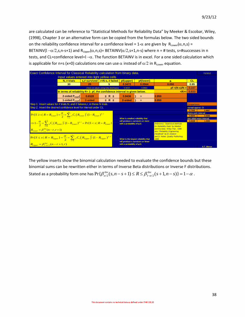
9/23/12

38

Exact Confidence Interval for Classical Reliability calculation from binary data. 7/2/2012

Input values entered into light yellow cellsN, # trials s,# survived r=N-s, # failed pf(upper) pf(lower) CL

30 25 5 0.3472 0.0564 0.050 0.95

check on values using beta distribution 0.3472 0.0564 pf =(N-s)/N = 0.167

In terms of reliability R= 1- pf, the confidence interval is given below. <R>= 0.833

2-sided Pexact{ 0.6528 ≤ R ≤ 0.9436 } = 0.950

1-sided Pexact{ 2-sided ≤ R ≤ 2-sided } = 0.950

Step 1: Insert values for # trials,N, and # failures,r, in those N trials Comparisons

Step 2. Insert the desired confidence level for interval under CL normal approx. CI

0.7000 0.9667

Score conf. Interval

0.6644 0.9266

What is smallest reliability that two sided exact interval

will produce s survivors or more 0.6528 1.0000

with a probability of /2. Reference: "Statistical Methods

for Reliability Data" by Meeker

and Escobar, Wiley Pub., 1998

also "Reliability Engineering

Handbook" by B. Dodson

and D. Nolan, Quality Publishing

What is the largest reliability that 1999

will produce s survivors or fewer

with a probability of /2.

A.T. Mense

0

1 /2

Pr{ | } (1 )2

( 1, )

s

in i

Upper n i Upper Upper

i

Inv

Upper

S s R R C R R

R n r r

/2

1

0

Pr{ | } (1 )2

1 (1 ) Pr{ | }2

( , 1)

ni n i

Lower n i Lower Lower

i s

si n i

n i Lower Lower Lower

i

Inv

Lower

S s R R C R R

C R R S s R R

R n r r

are calculated can be reference to “Statistical Methods for Reliability Data” by Meeker & Escobar, Wiley,

(1998), Chapter 3 or an alternative form can be copied from the formulas below. The two sided bounds

on the reliability confidence interval for a confidence level = 1- are given by RLower(n,s) =

BETAINV(1/2,s,n-s+1) and RUpper(n,s)= BETAINV(/2,s+1,n-s) where n = # tests, s=#successes in n

tests, and CL=confidence level=1. The function BETAINV is in excel. For a one sided calculation which

is applicable for n=s (x=0) calculations one can use instead of /2 in RLower equation.

The yellow inserts show the binomial calculation needed to evaluate the confidence bounds but these

binomial sums can be rewritten either in terms of Inverse Beta distributions or Inverse F distributions.

Stated as a probability form one has /2 1 /2Pr{ ( , 1) ( 1, )} 1Inv Invs n s R s n s .

9/23/12

39

1 ( )( ),

( )

0 ,

xx ex

f x

x

2 2

3 1 4 2

/ mean, mode= +( -1)/ , / variance

3 22coef of skewness ,coef of kutosis

Appendix D. Useful Probability Distributions.

Beta. The function B(a,b) is the complete beta function, parameters (a, b).

( , ) ( ) ( ) / ( )B a b a b a b and G is of course the gamma function 1

0

( ) t xx e t dt

.

(1 ) 1 1(1 ) (1 )( | , ) (general form)

( 1, (1 ) 1) ( , )

1[ ] ,

2

m mN N

m m

m

m

R R R Rf R Nm

B N N B

NE R

N

Mode

In the above distribution think of the parameter, Nm, as a measure of accuracy. High values of Nm imply that the modal (peak) reliability is a very good estimate. A large Nm will produce a

very peaked fprior(R=) and more experimental data will be needed to over come the prior.

Gamma.

This distribution is the general case for many useful distributions in

statistics. Sometimes is taken as the reciprocal of its use here.

Note: =0, =1/2, = k/2 produces the Chi Square distribution 2(dof=k) with degrees of

freedom = k.

9/23/12

40

21

21( )

2

x

f x e

Normal & Standard Normal The normal or Gaussian distribution is widely used either in its natural form or in a normalized for call a standard

normal or unit normal in which the mean=0 and the variance = 1. The equation is shown below for both

formulations note: z = (x – )/.

With =mean and =standard deviation. One can normalize the distribution in a very useful way so that any data

can be plotted in a dimensionless form. This produces what is called the standard normal distribution and it is used

so much that it carries its own special symbol, (z). Only the normal distribution and the student t distribution

benefit from this variable transformation i.e ( ) /z x and ( ) /t x x s where x is the sample mean

and s is the sample standard deviation.

Appendix E. Derivation of Time Dependent Posterior Distribution (See Hamada et al. Chapter 4 section 3)

Typical of many reliability analyses one assumes and exponential time-to-first-failure distribution whose failure rate

parameter (hazard function) is . In Bayesian analysis all parameters are assumed to be random variables that are

described by distribution functions. This will be done for .

Consider the prior distribution model for given by a Gamma() probability density function as shown below

1( )( ) , , , 0prior

eg

Why use a Gamma distribution? Experience in Bayesian modeling has shown that gamma distributions are

reasonable representations for failure rates as they provide a spread of values from which the Likelihood function

can emphasize the values needed to fit the data. That is - the data will select which values of the prior distribution

are the most important. Sometimes we have to go back and adjust the prior distribution based on where the data

may be taking us. This is called dynamical updating.

The likelihood function for a n tests where each test is conducted until there is a failure (i.e. no censored times) with

the respective failure times recorded as ti, i=1,2,…,n is shown below. (This can be easily generalized to account for

censored data)

Define the total time on test as

1

n

i

i

T t

, the likelihood function can be written as

1

( | , ) i

nnt T

i

L data e e e

and the resulting posterior distribution is given by multiplying

the prior times the likelihood and produces, 1

( | , ) ,( )

n T n

posterior

T e eg data T n

n

which

becomes, after normalizing, a gamma distribution, Gamma(n+, +T-n).

1

1

( | , )

n

i

i i

n tnt

i

L data e e e

21

21

( )2

z

f z e z

9/23/12

41

Appendix F. Markov Chain Monte Carlo Process (Hamada et al., Chapter 3, section1)

Bayesian analyses requires high-dimensional integration and this prevented the widespread adoption of Bayesian

techniques.

Appendix G. Likelihood Functions This concept originated (I believe) with Sir Ronald Fisher in England in the early 1900’s and has been very useful in

establishing estimates of population parameters based upon data and some presumed form of a distribution function.

Let me assume for the moment we place n units under test. All n unts are tested for a time tR and either the unit has

failed prior to tR (at a time tk let’s say) or it is still successfully operating at time tR. We will call the units that have

not failed by time tR censored data and tR the censored time. So if I total up all the time on test of all n units I obtain

what is called Total Time on Test (TTT) =

#

1

( )r failedunits

k R

k

t n r t

, and is a measure of time to first failure.

With these definitions let me also assume that a Weibull distribution is used to model these failure events. The

Weibull has 3 parameters (=scale parameter, =shapre parameter, =location parameter), The form of the

distribution is

1

( | , , ) exp , for t

( | , , ) 1 exp , for t

Weibull

Weibull

t tf t

tF t

and for the sake of simplicity I

will take =0 for the calculations that follow.

Now consider the following line of reasoning: if a unit fails at time tk the probability (likelihood) that this failure

would occur is proportional to the pdf evaluated at the “known” time tk, i.e. probability ~f(tk). Say we have r failures

prior to time tR. There is a failure at time t1 AND a failure at time t2 AND a failure at time t3 AND etc. out to time tr

AND there is no failure for unit r+1 AND no failure for unit r+2, etc. out to unit n. This can be written as

L(r|n,)=

1

failed units 1 censored units 1 1 1

( | , ) ( | , ) exp expr n r n

k k lWeibull k Weibull l

k l r k l r

t t tf t F t

This product is called the likelihood function and it uses the multiplication rule from basic probability theory to

construct it. It is proportional to the probability that you find r failures at the given failure times and (n-r) non-

failures at time tR when testing n units for time tR.

If you were to construct two partial derivatives of L e.g. ,L L

and set each expression equal to zero you would

have 2 equations in 2 unknowns () and in principle you can solve those equations for alpha and beta. The values

so obtained are call Maximum Likelihood Estimators or MLE for the parameters and .

For your personal edification the values of these MLE are given on Reliasoft’s web site as well as on Wikipedia and

in several texts.

While I have shown an example of finding a likelihood function for the random variable t or time to failure, it is

easy to see that the concept of likelihood is very general and can be applied to many situations of interest. It will be

extensive used in Bayesian analyses.

9/23/12

42

Weibull Analysis: (Taken from Robert Abernathy’s Text) What: Weibull analysis is the tool of choice for most reliability engineers when they

consider what to do with age-to-failure data. It uses the two-parameter Weibull

distribution which says mathematically that reliability, R(t) = e-(t/)^

where t is time,

is a scale factor known as the characteristic life (most of the Weibull distributions

have tailed data and lack an easy way to describe central tendency as the

mode≠median≠mean; however, regardless of the -values, which is a shape factor, all

of the cumulative distribution function values pass through the value at 63.2%

which thus entitles it to be known as the single-point characteristic life).

Be careful in use of the three-parameter Weibull equation! It is frequently misused

simply to get a good curve fit! The three-parameter Weibull requires compliance

with these four requirements:

1) you must see curvature of data on a two-parameter plot (concave downward

curves imply a failure free interval on the age-to-failure axis whereas concave upward

curves imply a percentage of the population are pre failed),

2) you must have a physical reason for why a three-parameter distribution exists

(producing a better curve fit is not a valid reason!),

3) you must have at 21 failure data points (if curvature is slight you may need 100+

data points), and

4) the goodness of curve fit must be significantly better after use of the three-

parameter distribution.

Why: The Weibull distribution is so frequently used for reliability analysis because one set

of math (based on the weakest link in the chain will cause failure) describes infant

mortality, chance failures, and wear-out failures. Also the Weibull distribution has a

closed form solution:

1) for the probability distribution function (PDF),

2) for the cumulative distribution function (CDF),

3) for the reliability function (1-CDF), and

4) the instantaneous failure rate which is also known as the hazard function.

For engineers, discrete solutions are preferred rather than use of tables because of

simplicity. In a similar manner, engineers strongly need graphics of the Weibull

distribution whereas statisticians do not find the graphics nearly as useful for

comprehension.

When: Use Weibull analysis when you have age-to-failure data.

When you have age-to-failure data by component, the analysis is very helpful

because the -values will tell you the modes of failure which no other distribution

will do [<1 implies infant mortality with decreasing failure rates, ≈1 implies

chance failures with a constant failure rate, and >1 implies wear-out failure modes

with increasing failure rates—when you know the failure mode you know which

“medicine” to apply]!

When you have age-to-failure for the system, the -values have NO physical

significance and the -, -values only explain how the system is functioning—this

means you loose significant physical information for problem solving.

Where: When in doubt, use the Weibull distribution to analyze age-to-failure data. It works

with test data. It works with field data. It works with warranty data. It works with

accelerated testing data. The Weibull distribution is valid for ~85% to 95% of all life

9/23/12

43

data, so play the odds and start with Weibull analysis. The major competing

reliability distribution for Weibull analysis is the lognormal distribution which is

driven by accelerating events. For additional information read The New Weibull

Handbook, 5th

edition by Dr. Robert B. Abernethy and use the SuperSMITH

Weibull and SuperSMITH Visual software for analyzing the data.

References: [1] Johnson, Graves, Hamada & Reese, A hierarchical Model for Estimating Complex System Reliability, ( submitted to 7th Valencia International Meeting on Bayesian Statistics, June 2-6, 2002, Tenerife, Spain) Los Alamos report, LA-UR-01-6915, (Dec 20, 2001). [2]Martz & Waller, “Bayesian Reliability Analysis,” Wiley & Sons, (1982). [3] Hamada, Wilson, Reese & Martz, “Bayesian Reliability,” Springer, (2008). [4] Meeker & Escobar, “Statistical Methods for Reliability Data,” Chapter 14, Wiley, (1998) [5] Kruschke, “Doing Bayesian Data Analysis,” Academic Press – Elsevier,(2011) [6] http://www.itl.nist.gov/div898/handbook/apr/section1/apr1a.htm [7] Hamada, Wilson, Reese & Martz, “Bayesian Reliability,” (2008), Springer, Chapter 3. [8] Ntzoufras, “Bayesian Modeling Using WinBUGS,” (2009), Wiley, Chapter 2. [9] Hoff, “A First Course in Bayesian Statistical Methods,” (2009), Springer, Chapters 4,6,10 [10] Law, “Simulation Modeling & Analysis, 4th Ed.,”(2007),McGraw-Hill, Chapter 8 [11] Gelman, Carlin, Stuart & Rubin, “Bayesian Data Analysis, 2nd Ed.,” Chapman & Hall/CRC Press [12] Resnick & Hardisty, “GIBBS SAMPLING FOR THE UNINITIATED,” paper from presentation at U. of Maryland workshop June 2010, CS-TR-4956, UMIACS-TR-2010-04, LAMP-TR-153 available at URL: (www.umiacs.umd.edu/~resnik/pubs/gibbs.pdf) [13] Smith, A. F. M. 1991. Bayesian computational methods. Phil. Trans. R. Soc. Lond. [14] Evans, M., and T. Swartz. 1995. Methods for approximating integrals in statistics with special emphasis on Bayesian integration problems. Statistical Science 10: 254–272. [15] Tanner,M.A. 1996. Tools for statistical inference, 3rd ed. Springer-Verlag, New York. [16] Gelfand, A. E., and A. F.M.Smith. 1990. Sampling-based approaches to calculating marginal densities. J. Am. Stat. Asso. 85: 398–409. [17] Metropolis, N., and S. Ulam. 1949. The Monte Carlo method. J. Amer. Statist. Assoc. 44: 335–341. Metropolis, N., A.W. Rosenbluth, M. N. Rosenbluth, A.Teller, and H. Teller. 1953. Equations of state calculations by fast computing machines. Journal of Chemical Physics 21: 1087–1091. [18] Geman, S. and D. Geman. 1984. Stochastic relaxation, Gibbs distribution and Bayesian restoration of images. IEE Transactions on Pattern Analysis and Machine Intelligence 6: 721–741. [19] Draper, David. 2000. Bayesian Hierarchical Modeling.

9/23/12

44