BAYESIAN STATISTICS AND PRODUCTION RELIABILITY

• ASSESSMENTS FOR MINING OPERATIONS

by

Gaurav Kumar Sharma

B.E., Thapar University (India), 2003

A THESIS SUBMITTED iN PARTIAL FULFILLMENT OF

THE REQUIREMENTS FOR THE DEGREE OF

MASTER OF APPLIED SCIENCE

in

The Faculty of Graduate Studies

(Civil Engineering)

THE UNIVERSITY OF BRITISH COLUMBIA

(Vancouver)

April 2008

© Gaurav Kumar Sharma, 2008

Abstract

This thesis presents a novel application of structural reliability concepts to assess the

reliability of mining operations. “Limit-states” are defined to obtain the probability that the

total productivity — measured in production time or economic gain — exceeds user-selected

thresholds. Focus is on the impact of equipment downtime and other non-operating instances

on the productivity and the economic costs of the operation. A comprehensive set of data

gathered at a real-world mining facility is utilized to calibrate the probabilistic models. In

particular, the utilization of Bayesian inference facilitates the inclusion of data — and

updating of the production probabilities — as they become available. The thesis includes a

detailed description of the Bayesian approach, as well as the limit-state-based reliability

methodology. A comprehensive numerical example demonstrates the methodology and the

usefulness of the probabilistic results.

11

Table of Contents

Abstract.ii

Table of Contents .. iii

List of Tables iv

List ofFigures v

List ofSymbols vii

List ofAbbreviations viii

Acknowledgements ix

1 Introduction 1

1.1. Literature Review 4

2 Data Analysis For Mining Equipment 7

2.1. The Nature of the Raw Data 8

2.2. Modeling of Equipment States 13

2.3. Treatment of Uncertainty: A Bayesian Approach 16

2.4. The Predictive Analysis 20

3 Reliability Analysis 45

3.1. Reliability Formulation 46

3.2. Results and Applications 533.2.1. Production Time 543.2.2. Economic and Unscheduled Repair Costs 57

4 Discussion and Jonclusions 76

References 77

A PPENDIXA 80

A.1 Random Variable 81

A.2 Cumulative Distribution Function 82

A.3 Probability Mass Function 83

A.4 Probability Density Function 84

A.5 Types of Uncertainties 85

A.6 Basic Stochastic Processes 86A.6.l The Bernoulli Sequence 86A.6.2 The Poisson Process - Random occurrence model 89

APPENDIX B 90

111

List of Tables

Table 1: Classification of equipment states 24

Table 2: Type of components for repairs 25

Table 3: Number of repairs observed in a year for the four equipments 25

Table 4: Time between successive scheduled repair events (in days) 26

Table 5: Statistics for time between successive UR sub-states 26

Table 6: Probability distributions for duration in sub-state for various equipments 27

Table 7: Bayesian procedure to obtain updated occurrence rate(2uR) for equipment no. 6161.

28

Table 8: Bayesian procedure to obtain updated occurrence rate(2uR) for equipment no. 6162.

29

Table 9: Bayesian procedure to obtain updated occurrence rate(2uR) for equipment no. 6163.

30

Table 10: Bayesian procedure to obtain updated occurrence rate(2uR) for equipment 6164. 31

Table 11: Bayesian updated mean occurrence rate for the random non-operating sub-states of

equipments 32

Table 12: Costs associated with different states of functioning of equipment 61

Table 13: Empirical Productivity and Economic Cost Data 61

iv

List of Figures

Figure 1: Excerpts from a typical equipment dispatch report 33

Figure 2: Relative frequency histogram, exponential and lognormal PDF for the time

between successive UR sub-states 34

Figure 3: Cumulative frequency histogram, Exponential and Lognormal CDF for the time. 35

Figure 4: Relative frequency histograms for UR sub-state duration 36

Figure 5: Cumulative frequency plot for the UR sub-state duration 37

Figure 6: Lognormal fit for the duration (time in state - TIS) of UR sub-state 38

Figure 7: An example of a time-window with several state transitions 40

Figure 8: Poisson probability mass function using a point estimate of rate of occurrences of

UR sub-state 41

Figure 9: Number of Poisson occurrences with predictive and point estimation of sub-state

occurrence rate for equipment 6161 42

Figure 1 0 Predictive-CDF plot for the failure of equipment number 6161 43

Figure 11: Reliability plot for equipment 6161, Occurrence rate 0.4 44

Figure 12: Methodology of calculating the total time in non-operation, TNO(x) for an

equipment 62

Figure 13: Flowchart illustrating an algorithm for sampling time spent in non-operating state

63

Figure 14: Sampling results - PDF plot for the total production time (units: truck-days) of the

four HEMM equipments in half-year 64

V

Figure 1 5: Sampling results - CDF plot for total production time (units: truck-days) of the

four HEMM equipments in half-year 65

Figure 16: PDF plot for the total production time (units: truck-days) of the four HEMM

equipments in one-year 66

Figure 17: Sampling results - CDF plot for total production time (units: truck-days) of the:

four HEMM equipments in one-year .67

Figure 18: PDF plot for the total production time (units: truck-days) of the four HEMM

equipments in two-years 68

Figure 19: Sampling results - CDF plot for total production time (units: truck-days) of the

four HEMM equipments in two-years 69

Figure 20: Sampling results - PDF plot for total economic and repair costs (units: $ million)

of the four HEMM equipments in half-year 70

Figure 21: Sampling results - CDF plot for total economic and repair costs (units: $ million)

of the four HEMM equipments in half-year 71

Figure 22: Sampling results - PDF plot for total economic and repair costs (units: $ million)

of the four HEMM equipments in one-year 72

Figure 23: Sampling results - CDF plot for total economic and repair costs (units: $ million)

of the four HEMM equipments in one-year 73

Figure 24: Sampling results - PDF plot for total economic and repair costs (units: $ million)

of the four HEMM equipments in two years 74

Figure 25: Sampling results - CDF plot for total economic and repair costs (units: $ million)

of the four HEMM equipments in two years 75

vi

List of Symbols

• 2UR Mean occurrence state rate of the unscheduled repair sub-state

T Total Observation Period

TNQ(x) Vector of random variables for time in non-operation

To(x) Vector of random variables for time in operation

x Name ofa state

Time of Occurrence of state, x

• d Duration of state, x

Mean occurrence state rate of state, x

N Number of Poisson occurrences of state, x

k Parameter 1 of Gamma distribution

v Parameter 2 of Gamma distribution

p2 Mean of occurrence rateCoefficient of variation of occurrence rate

Tbf Time-between-failures

T9 Time threshold

g(x) Expression for limit-state function

N Total number of sub-states

C Normalizing constant

Cop Operating cost of equipment per unit time

CUR Unscheduled repair cost of equipment per unit time

CSR Scheduled repair cost of equipment per unit time

CE Economic (Opportunity) cost of equipment per unit time

C(x) Vector of random variables for economic and repair cost

C Cost thresholdTotal time spent in random state x in the observation period

D Total time spent in deterministic state in the observationperiod

C Normalizing Constant

E An event

F(2) Probability density function for occurrence rate, 2

f ‘(2) Prior distribution for 2

F “(2) Posterior distribution for 2

P(AIB) Conditional probability that event A will occur given thatevent B has occurred

L(2) Likelihood function for 2

vii

List of Abbreviations

PDF Probability Density Function

CDF Cumulative Distribution FunctionPMF Probability Mass Function

HEMM Heavy Earth Moving Machinery

UR Unscheduled Repair

viii

Acknowledgements

I would like to acknowledge the assistance, support and encouragement that have been

provided by the following people and institution, without whom, this research would not

have been possible.

• Dr. Terje Haukaas

• Dr. R. A. Hall

• Highland Copper Valley Mine

• The University of British Columbia

• Natural Sciences and Engineering Research Council of Canada, Collaborative

Research and Development Grants

I owe particular thanks to Dr. Haukaas, whose enthusiasm and dedication towards his work

and students will always inspire me in my career ahead.

Special thanks are also owed to my parents and my wife for supporting me in my education.

ix

1 Introduction

The objective of this thesis is to combine statistical analysis of data recorded at a real mining

site with modern reliability methods to predict the future productivity of a mining operation.

Focus is on the impact of equipment downtime and other non-operating instances on the

productivity and the economic costs of the operation. The probability of equipment bcing

non-operative is influenced by a number of uncertain factors. These include local weather,

geological conditions, human factors, uncertain degree of machine deterioration, and inherent

uncertainty in material and equipment quality. For example, equipment may become

intermittently non-operative due to poor weather conditions such as snow, rain, low visibility,

and excessive humidity. Similarly, varying geological conditions such as difficult

mountainous terrain, rocks and boulders inflict higher-than-normal equipment deterioration;

thus increasing the likelihood of breakdown. Human factors such as delays, non-availability

of operator, inadequate equipment handling, and comprehensive equipment usage also may

result in a higher number of non-operative instances, leading to low operational reliability.

In today’s modern mining setups, real time data gathering systems are installed on

equipment in order to monitor the various states of equipment operation. The data, upon

analysis, serves to provide necessary feedback for strategic decision-making. For example,

the data supports decisions concerning operational processes, production output, öost

management, etc. The methods presented in this thesis provide novel tools for analyzing the

equipment production data and for reliability assessment of production.

The case under consideration is the hauling of ore using heavy earth moving

machinery (HEMM). This equipment is increasingly deployed because of their large hauling

1

capacity. This yields time-saving during loading compared to using smaller equipment, and

carries reduced operator cost. However, the risk of deploying HEMM equipment is larger

because of the high consequence of failure of one HEMM. It is necessary that downtimes and

idle-time (time in non-operation) of such equipments are minimal because loss of production

results in high economic costs. Importantly, the overall cost of an earth moving mining

operation is significantly affected by the reliability of the HEMM equipments used in the

operation. Lower reliability of the equipment alters productivity and drives the maintenance

and operating costs; thus affecting profit margins. This motivates the focus on productivity

and cost-based limit-states in the subsequent reliability analysis.

A comprehensive set of observations gathered at the Highland Valley Copper mine

(Priyadarshini et al. 2005) are processed into a database and subjected to Bayesian statistical

analysis. The observations include the occurrence and duration characteristics of the various

states of functioning of a set of HEMM equipments. The database classifies the observations

according to the stochastic properties of the states. The preliminary analysis of data is dOne

using probabilistic modeling of occurrence and duration patterns of the different states of

equipment functioning. Homogeneous Poisson process is adopted as the random occurrence

model. Bayesian inference is used for addressing the uncertainty in occurrence rates of the

equipment states. The utilization of Bayesian inference facilitates the inclusion of data — and

updating of the equipment state occurrence rates — as they become available. The thesis

includes a detailed description of the Bayesian approach. The results of the Bayesian analysis

include Statistics for the occurrence of various states of equipment functioning, which

subsequently enter into a reliability formulation.

2

The reliability analysis comprises innovative utilization of concepts of structural

reliability analysis to assess the production probabilities of the mining operation. Structural

reliability problems, such as design code calibration and assessment of failure probabilities of

structures are solved using a limit-state-based methodology. A limit-state function is a

mathematical expression to represent an event of interest. The limit-state function is

designated by g(x), where x is a vector of random variables. Negative and positive values of

g signify the failure state and the safe state, respectively. The reliability of system is

determined by first computing the failure probabilities of system components. Then the

various failure modes (limit-states) of the components are determined. The reliability of the

components is computed by integrating the joint probabilities of load and resistance over the

failure domain, which is defined by g(x) 0 (Melchers 1999). Typically, the system is either

a series system of parallel sub-systems (sub-parallel systems known as “cut sets “) or parallel

system of series system (known as “link sets”). The overall system reliability is obtained

from the failure probabilities of system components constituting the cut-sets.

In this thesis, limit-state-based reliability formulations are developed to study the

impact of equipment downtime and other non-operating instances on the production times

and the economic costs (loss of opportunity) of operation. In particular, limit-state functions

are defined to obtain the probability that the total productivity — measured in production time

or economic gain — exceeds user-selected thresholds. It is noted that the presented reliability

formulations also provide a novel way of addressing the system reliability problem. In order

to assess production reliability of a fleet of equipment, the contribution to production from

the equipment is calculated by considering equipment downtime and idle-time in contrast to

3

considering the explicit failure or non-failure combinatorial of the equipment. This

circumvents the traditional system reliability problem.

1.1. Literature Review

Today, large-sized mining equipment are increasingly being used for ore-hauling process.

This is primarily to increase productivity and reduce operational costs of the process. The

impact of sudden failures of such large and complex equipments on the cost and production

is significant. Mitigation of this necessitates improvement in the assessment techniques of

equipment reliability. In the following, the state-of-the-art in the field of reliability

assessment of mine equipment productivity is discussed.

Reliability is defined as the probability that a unit will perform its intended function

until a specified point in time under encountered use conditions. Importantly, the

environment in which a product operates is a critical factor in evaluating a product’s

reliability (Meeker and Escobar 2004, p.1). Availability is the probability that the unit is

operating properly when its use is intended, i.e., it is not undergoing repair action, etc.

Maintainability is the ability of the unit to be retained in, or restored to a specified state when

the maintenance action is performed on the unit. The three concepts are interlinked and form

the primary standard in reliability-availability-maintainability (RAM) based approaches for

acquiring quality products (Department of Defense 2005).

Specific studies have been performed to analyze the impact of heavy ore-hauling

equipment on mine production. One such method described by Yuriy and Vayenas (2007)

involves reliability assessment of load-haul-dump using genetic algorithms and discrete event

simulation models. A typical mine development cycle is emulated for analyzing the effect of

4

load-haul-dump equipment failures on production throughput, mechanical availability and

equipment utilization. Gupta et al. (1999) describe a method for analyzing productivity of

surface mining systems. According to the method, a production process remains in only one

of two states: working or non-working. Transition from one state to the other is defined as a

stochastic process and the state probabilities of the process are determined using the Markov

modeling:technique.

The production attained from an equipment is dependent upon the reliability: of

equipment, which is dependent on factors including the operating environment of equipment,

equipment’s maintenance quality, its handling, etc. Vagenes and Nuziale (2001) present a

reliability assessment model based on genetic algorithms, which considers the dependence of

equipment reliability on equipment’s age, operating environment, number and quality of

repairs for mining equipment. Impact of these factors is incorporated in a genetic algorithm

to assess equipment reliability and predict future time-between-failures.

An important basis for reliability computations is the collection and analysis of

appropriate data. Methodologies for gathering and analyzing reliability data in mining

environment are well developed (Hall and Daneshmend 2003). Meeker and Escobar (2004)

describe the use of Bayesian techniques for analyzing failure data. The analysis involves

combining prior information with available field data for quantifying the uncertainty.

Apeland et al. (2003) combine a Bayesian approach and Monte-Carlo simulation techniques

to deal with component failures.

The concept of delay-time considers a component to be present in one of the three

states, i.e., non-defective, defective state and failure state. Failure propagation involves

changes of state between non-defective to defective state and then into failure state. Delay

5

time is the time spent by the equipment from defective to failure state, if it is not inspected.

Apeland et a!. (2003) describe approaches for modeling inspection times, time to defect and

delay-times using fully subjective (Bayesian) approach and Monte-Carlo simulation

techniques.

The impact of equipment downtime on the cost of operation is an area of great

interest for mine planning engineers. Vorster and Garza (2008) present a detailed

methodology for quantifying and categorizing the different costs associated with equipment

downtime and lack of availability. The cost impacts of failure of an equipment on the

productivity and cost effectiveness of other equipments and cost impact of capital assets

becoming idle due to equipment downtime are two of the consequential cost quantities

addressed by the authors. In particular, significant literature relating to reliability assessment

of mining equipments is available when compared to the reliability assessment of production

from a mine process.

The remainder of this thesis is organized into two major sections. The first section

comprises data analysis. The second section investigates plausible reliability formulations to

study the impact of equipment non-operation on the economic costs and production time.

This section also discusses the results and application areas of the analyzed data and the

reliability formulations.

6

2 Data Analysis For Mining Equipment

The first part of this thesis consists primarily of analyzing data relating to the various states

of functioning of mining equipment used in hauling of ore. In particular, the equipment in

consideration is a fleet of HEMM — Caterpillar Mining Truck-793®, which operate in an

open-pit mine of the Highland Valley Copper Inc.©. For identification, the equipments have

been assigned with unique numbers, 6161, 6162, 6163, and 6164. The preliminary data used

in the presented analysis was initially gathered by Priyadarshini et al. (2005) at the Highland

Copper Valley mine for determining the equipment failure and repair patterns.

In the following, the data has been analyzed to obtain probabilistic measures for the

various states of functioning of mining equipment. The probabilistic measures include the

number of occurrences of each state and the duration spent by equipment in each instance of

state occurrence. Subsequently, the probabilistic information obtained from the analyzed data

will serve as input to develop a cost and productivity-based reliability model. The reliability

model would assist the decision making process in mining operations.

Section 2.1 describes the nature of preliminary data; section 2.2 describes the

approach taken for classification of data and modeling of equipment states. Section 2.3

presents the key concepts used for probabilistic modeling of data along with the various

practical challenges in modeling such a system. Section 2.4 includes a detailed description of

Bayesian analysis of data for determining statistics for the rates of occurrence of different

states of equipment functioning along with the initial results. Finally, section 2.5 explores the

predictive analysis for interpreting analyzed data and applying it to draw useful inferences.

7

2.1. The Nature of the Raw Data

The data that are available for this study essentially consist of an annual dispatch report (time

log) of the operational status of equipments recorded at the mining site. The data comprises

status changes of equipment recorded continually in the form of date, time, duration, and the

nature of occurrence. The status of equipment functioning is categorized on the basis of

various types of events at the mine site such as, tie-down, standby, repair, non-operating

event, etc. This categorization has been adopted during the initial data gathering performed at

the Highland Valley Copper mine (Priyadarshini et a!. 2005).

Figure 1 shows excerpts from a typical equipment dispatch report. The first row

contains explanations of the different columns. The first five columns in the figure contain

the equipment number, date, time, duration of an equipment status, and name of the

equipment status. The remaining columns contain a code for the equipment status, category

of equipment functioning corresponding to the status, reason for non-operation of the

equipment, and comments for the equipment category. The equipment status changes several

times within a short span of time, with each status lasting for certain duration. For example,

operating status of the equipment is followed by non-operating instances resulting in a delay,

stand-by, operating delay, or a repair status. Hereinafter, in this thesis, ‘equipment status’ is

referred as ‘equipment state.’

Significant amount of data is available for analysis. There are approximately 65,000

instances of state changes for each equipment within a year. The data gathering methodology

adopted by Priyadarshini et al. (2005) provides the flexibility of analyzing the occurrence and

duration characteristics of different sub-states of the equipment. In order to model the

stochastic characteristics of the various states of functioning of the equipment, the annual

8

equipment dispatch report generated at the Highland Copper Valley mine has been proces:sed

into a comprehensive database. This database is included in the CD-ROM that is attached to

this thesis as Appendix B. The database includes occurrence and duration patterns: of

equipment states observed over one year. In particular, the database contains the number of

observations of each sub-state, the time between successive sub-state occurrences, and :the

durations of sub-states for each of the four equipment. The database is obtained by

processing the annual dispatch reports for the equipments.

Table 1 provides a complete classification of equipment states derived from the

database. According to the classification, the state of equipment functioning is broadly

categorized into operating and non-operating state. The non-operative state is sub-

categorized into various mutually exclusive sub-states, with each sub-state getting triggered

due to similar type of events. The advantage of such a discrete classification approach is the

separation of sources of uncertainty associated with respective sub-states. It is observed in

Table 1 that the sub-states are grouped under delay, operating delay, standby, scheduled

repair and unscheduled repair (UR). For example, delay in operation of equipment (a non-

operating state) resulting from a blasting event in the mine is classified as sub-state blast-

delay under the category operating delay. The fourth column in Table 1 lists the occurrence

patterns of different sub-states. Accordingly, the occurrence of a sub-state is either random or

deterministic in nature. The occurrence pattern of an equipment sub-state is based on the

nature of event that results in the equipment sub-state. For example, sudden equipment

failure is a random event, resulting in the random non-operating UR sub-state. On the

contrary, a daily lunch-break event results in a deterministic non-operating delay equipment

sub-state.

9

In the following, the equipment repair data from the dispatch report is processed as an

example for the overall data analysis approach. The equipment (HEMM) in consideration is a

large and complex piece of machinery and includes a number of components, some of which

are detailed in Table 2. One or more of these components malfunction or fail to cause entire

equipment breakdown and necessitating the repair. Therefore, it is difficult to assess the

exact time and cause of a component failure. In this study, the failure of one or more

components that resulted in a repair action is considered as a failure event. The details of the

time and durations of the repairs are obtained from the dispatch report, which includes two

types of events:

• Repairs performed on the equipment according to a scheduled maintenance

program;

• Repairs necessitated as a result of sudden failure of one or more component of the

equipment.

The latter event is random in nature and has been assumed to be a failure event in the

statistical studies. In other words, URs caused due to a sudden failure of one or more

components is a failure event. It is noted that during a failure event, more than one

component may have been repaired. Table 3 lists the number of repairs observed in a year for

the four trucks. The first column of the table lists the equipment number, the total number of

unscheduled repairs, and the total number of scheduled repairs observed over one year. it is

observed that equipment 6163 and 6164 needed more repairs than 6161 and 6162 in the

observation period. The likely reasons for this variation include equipment age, handling,

amount of usage, the quality of manufacturing, etc. In the next few paragraphs, the

occurrence and duration characteristics of the UR sub-state are discussed.

10

Table 4 lists the time (in unit of days) between successive scheduled repairs for the

four equipments. This data is obtained from the annual dispatch reports for the equipments. It

is clear from the table that successive scheduled repair events occur every 3 0-40 days

according to a preventative maintenance program. Therefore, the occurrence of scheduled

repair is deterministic in nature.

The time between UR sub-states is calculated by taking the difference between the

start times of successive UR events. In order to determine the probabilistic characteristics of

the occurrences of UR sub-states, the distribution of time between unscheduled repairs of the

equipments is studied. The nature of this distribution will aid in determining an appropriate

random occurrence model for equipment failures. For this, first the preliminary data is

analyzed in order to obtain the distribution for time between UR sub-states. To provide an

idea of the nature of the data, a few preliminary statistical measures for the time between UR

sub-states are provided in Table 5. For equipment 6161, the mean of the time between UR

sub-states is 6.3 days, with a standard deviation of 9.3 days, and a coefficient of variation of

148 %. Coefficient of variation for equipments 6162, 6163, and 6164 is close to 100%,

indicating high uncertainty in sub-state occurrence data. Reducing the uncertainty in time

between successive UR sub-states is one of the chief goals of the Bayesian methods

described later on in this section. Notably, as more data relating to UR sub-state occurrence

observations becomes available, the coefficient of variation reduces significantly, resulting in

less uncertainty.

Figure 2 shows a comparison between the frequency histogram, exponential

probability density function (PDF) and lognormal PDF of the time between successive UR

sub-states for the four equipments. Specifically, the bars in Figure 2 show the normalized

11

frequency histogram. The dashed and dotted lines are the exponential and lognormal PDFs

with the same measures. It is observed from the figure that time between UR sub-states is

mostly l3 days, i.e., a significant number of successive UR sub-state observations occur

within every 1-3 days. Furthermore, a comparison of frequency histogram with the

exponential and lognormal distribution reveals that exponential distribution is a reasonable fit

to the raw data.

Figure 3 shows the associated cumulative distribution functions (CDFs). The solid

line is the cumulative frequency; the dashed line is an exponential CDF with the

aforementioned mean and standard deviation. The dotted line is a lognormal CDF with the

same measures. It is observed that the lognormal and exponential distributions are reasonable

fits to the raw data. Notably, the slope of CDF points towards the uncertainty, or the spread

of data. A CDF with a steep slope indicates that the data is not highly dispersed (less

uncertainty), whereas, CDF with flatter slope points towards highly dispersed data (more

uncertainty). From Figure 3 it is clear that the time between UR sub-state data is less

dispersed for equipment 6161 than the other equipments. The Figure 2 also corroborates this

observation.

The duration characteristics of UR sub-state are discussed next. The time duration of

equipments in the UR sub-state is highly variable and uncertain. According to the database,

during a year, the total time spent in the UR sub-state by equipments 6161, 6162, 6263, and

6614 is 220, 227.17, 380.5, and 234.5 hours respectively. The maximum time durations of

the equipments in the UR sub-state are 42.3, 44.7, 58.9, and 107.2 hours respectively. Figures

4 and 5 show the spread of the UR sub-state duration data in the form of relative frequency

12

histogram and cumulative frequency. it is observed from Figure 5 that for almost 80% of;the

UR instances, 10 hours or less are spent by the equipments in the repair shop.

The duration data for UR sub-state is lognormally distributed. Accordingly, Figure 6

shows the lognormal distribution obtained for the data for the four equipments. These

distribution have been obtained using the Crystal Ball® software. Notably, the coefficient of

variation for the duration in UR sub-state is close to 200%.

2.2. Modeling ofEquipment States

A fundamental task in the present study is to estimate the time spent by equipment in non

operating states during an observation period. Probabilistic estimates of the time in non-

operation can be obtained from the occurrence and duration characteristics of equipment

states. The occurrence and duration patterns of many equipment states are random in nature,

due to the uncertainty associated with the event that causes the state. Conversely, there are

deterministic non-operating states due to events such as lunch, coffee break, which occur

according to a pre-defined schedule.

When an equipment transitions into a random state, the state lasts for a random

duration. For example, the occurrence of the UR sub-state and corresponding repair duration

are random. Figure 7 illustrates a time window in which a set of equipment state transitions

occur within a week. It is observed that the equipment undergoes scheduled repair for

preventative maintenance on day two, which lasts for ten hours and forty minutes, and then

operates for one and a half hour. Thereafter, a number of state transitions occur within the

next four-hour period, which is shown by zooming-in on the time axis. Within the zoomed-in

time window, the equipment operates intermittently with interruptions occurring due to

13

transition into various non-operating states. The non-operating states occur due to events

including lunch, blast delay, repair, crusher red lights on, short move, coffee break, and

operator shift change respectively. Hereinafter we denote the time of occurrence as t, where

x is the name of the state. Similarly, we denote the duration of the occurrence by d, where x

is the name of the state.

In the formulation developed in this thesis, a key quantity is the total time spent by an

equipment in a sub-state. For a given observation period, this duration is denoted D, where x

is the name of the sub-state. In a given observation period, D for a random sub-state is

uncertain. Therefore, in the proposed model, the number of occurrences, N, and

corresponding duration, d, of the random sub-state in the observation period are treated as

random variables. Given the realizations of these parameters for a random sub-state x, the

total duration in this sub-state, D, is evaluated by the expression

(1)

where N is the random number of occurrences of sub-state x within the given observation

time and d( is the random duration of occurrence number I. For deterministic sub-states, the

occurrence and duration parameters are pre-defined and the total time spent in the sub-state is

obtained by multiplying the total number of occurrences with the duration.

To model the uncertainty in number of occurrences N of random sub-state x, a

probabilistic occurrence model is used. The homogeneous Poisson process is an appealing

choice due to its simplicity. However, the implicit assumptions of independence between

occurrences and time-invariant statistical properties must be carefully examined. The Poisson

process is characterized by one parameter; the mean occurrence rate, 2. With knowledge of

this parameter, derived measures such as the probability distributions for number of sub

14

states in a time interval (the Poisson distribution) and time between sub-states (the

exponential distribution) become available. The probability of observing N occurrences in

observation period T is given by the Poisson probability mass function (PMF)

p(N)= (2T)NeT

(2)

The obvious approach to obtain a point estimate of 2 is to count the number of sub-states

within the time period and divide it by the total time. For example the mean occurrence rate

of unscheduled repairs, 2UR for equipments are essentially point estimates of the occurrence

rate. Figure 8 shows the PMF according to Eq. (2) for the point estimation of2UR for the four

equipment. The approach of point estimation of 2 has several weaknesses, including its

inability to obtain a measure of uncertainty in the estimate of 2. This is remedied in the

Bayesian approach suggested by Benjamin (1968). The Bayesian analysis is carried out inthe

next section to obtain probability distributions for 2 for a number of sub-states.

In this thesis, the probability distribution for the duration parameter d is not obtained

by Bayesian updating. Instead, probability distributions for d are selected by means of a

simple best-fit technique. For example, duration data for UR suggests that the lognormal

distribution is appropriate for all equipments under consideration. Similarly, the durations of

power outage is exponentially distributed. Likewise, appropriate standard-type probability

distributions for the durations of other sub-states of equipment are chosen. For this purpose, a

standard software is utilized to fit probability distributions to d for all the sub-states. Table 6

lists the best fitting distributions to d for the sub-states of equipment. The first row contains

explanations of the different columns for the equipments. The subsequent rows contain the

results from the fitting. For each equipment, the first, second and third columns respectively

15

provide the distribution type, the mean duration in unit of minutes, and standard deviation of

the sub-states. For many of the sub-states, a particular distribution type fits to the duration

data of all the equipment in consideration. The exponential distribution fits well to the

duration data corresponding to sub-states with very large variation in the magnitude, of

duration. For example, the durations of typical power outages varies from 20 minutes to 2000

minutes. Examples of other such sub-states include slippery/poor visibility, maintenance

foreman in vehicle, and no-dump available. Furthermore, it is observed that the duration data

corresponding to sub-states; no-operator available and UR has very high standard deviation.

This is expected because of the highly uncertain nature of such events in practice.

2.3. Treatment of Uncertainty: A Bayesian Approach

The objective of this section is to analyze the occurrence rate, 2, of the sub-states of mining

equipment. In the Bayesian approach, 2 is itself considered to be a random variable.

Importantly, the probability distribution for this random variable is repeatedly updated with

information about occurrences of sub-state. Such updating is performed on the database

gathered from the mining operation studied in this project. Before presenting the results, the

methodology is briefly reviewed. The basic version of Bayes’ theorem for the two events A

and B reads

P(AIB)= P(A) (3)P(B)

where P(AIB) denotes the conditional probability that event A will occur given that event B

has occurred. The significance of Eq. (3) is its ability to update the probability ofA in light of

the occurrence of event B. This is reflected in the Bayesian terminology, in which P(A) is

16

denoted the prior probability, while P(AIB) is the posterior probability, F(BIA) is the

likelihood function, and P(B) is a normalizing constant.

Bayes’ theorem applied to the PDF,f(2) of a random variable 2 reads

f(2 I E) = P(E12) f(2) (4)

where E is the event that influences the PDF of 2. It is more common to write Eq. (4) in the

form

f”(2)cL(2)f’(2) (5)

where f “(2) is the posterior PDF for the occurrence rate, c is a normalizing constant that

ensures a valid posterior PDF, L(2,) is the likelihood function that denotes the probability of

making the observation, and f ‘(2) is the prior PDF. Clearly, the objective of Eq. (5) is to

update the PDF of 2 in light of an observation whose information is implicitly incorporated

in the likelihood function. From the above it is also clear that the likelihood function

represents the probability of observing the observation given 2. Specifically, the probability

of observing N occurrences in a time interval T is, according to the Poisson process given by

the Poisson probability mass function explained in Eq. (2).

Consequently, the likelihood of observing, say, 3 equipment sub-states within a

period of 40 days, given 2, is proportional to 23e402 (it is not necessary to retain the entire

expression in Eq. (1), but only the terms that contain 2, because the normalizing constant c

will ultimately ensure a valid PDF).

The choice of prior PDF is part of the art of Bayesian updating. Typically, subjective

judgment enters into this choice. However, it is emphasized that the prior PDF has little

17

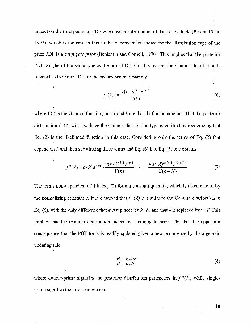
impact on the final posterior PDF when reasonable amount of data is available (Box and Tiao,

1992), which is the case in this study. A convenient choice for the distribution type of the

prior PDF is a conjugate prior (Benjamin and Cornell, 1970). This implies that the posterior

PDF will be of the same type as the prior PDF. For this reason, the Gamma distribution is

selected as the prior PDF for the occurrence rate, namely

f )= v(v.2)’e2

(6)X F(k)

where F() is the Gamma function, and v and k are distribution parameters. That the posterior

distributionf “(2) will also have the Gamma distribution type is verified by recognizing that

Eq. (2) is the likelihood function in this case. Considering only the terms of Eq. (2) that

depend on 2 and then substituting these terms and Eq. (6) into Eq. (5) one obtains

ftI(2)=c2Ne_2Tv(v.2)kev2=...= v(v.2)e_T)2

F(k) F(k + N)

The terms non-dependent of 2 in Eq. (2) form a constant quantity, which is taken care of by

the normalizing constant c. It is observed that f “(2) is similar to the Gamma distribution in

Eq. (6), with the only difference that k is replaced by k+N, and that v is replaced by v+T. This

implies that the Gamma distribution indeed is a conjugate prior. This has the appealing

consequence that the PDF for 2 is readily updated given a new occurrence by the algebraic

updating rule

8v”— v’+T

where double-prime signifies the posterior distribution parameters in f “(2), while single

prime signifies the prior parameters.

18

In summary, the prior distribution f ‘(2) indicates our state of knowledge about 2

before a particular sub-state observation is made for an equipment. The Bayesian updating

rule in Eq. (5) combines the prior information contained in f ‘(2) with new observations

contained in L(2). The posterior distributionf”(2) represents the updated state of information

about the mean sub-state occurrence rate 2. In passing, it is also noted that the mean,

standard deviation, and coefficient of variation are available from the Gamma distribution

for 2: Mean ,u, = k/v, standard deviation 02, k/v and coefficient of variation c = 1/k.

Bayesian analysis as described above is carried out for all random sub-states. In the

following, it is demonstrated for the occurrence of unscheduled repairs (sudden breakdown

of the equipment). The time between UR events is recorded in units of days. A significant

number of UR occurrences were recorded; typically in the order of 60 sub-states over a time

period of 12 months. The rate of unscheduled repairs is denoted 2(11?. Based on judgment, the

prior distribution for 2UR was chosen to have a mean equal to 0.167 occurrences per day with

a large degree of uncertainty; a 100% coefficient of variation was selected. This corresponds

to V’UR = 6 and k’u1? 1. It is reemphasized that this initial assumption usually has little impact

on the final distributionf’(2uR) for the occurrence rate.

As an example of the application of the methodology outlined in the previous section,

Tables 7, 8, 9, and 10 are provided. The tables present the Bayesian procedure for updating

the occurrence rates of UR sub-states for equipments 6161, 6162, 6163, and 6164. The first

row in each table contains explanations of the different columns and the second row contains

the initial assumption stated in the previous paragraph. The subsequent rows contain the

results from the Bayesian updating according to Eq. (8). Notably, as more and more

information on UR substates are incorporated, the coefficient of variation of the 2UR

19

distribution is reduced. As expected, this indicates that the incorporation of information

reduces the uncertainty in 2UR. The tables only shows very few of the UR occurrence

observations that are included in the database, for illustration purposes. The last row of each

table contains the graphs of the prior and posterior Gamma probability distributions f’(A)

which are plotted over a range of2UR values. The plot contains six PDFs; the five first PDFs

obtained during the Bayesian updating and the last, which is obtained after all the UR data, is

incorporated. It is observed that the initial PDFs have substantial dispersion, while the last

PDF is significantly narrower, thus indicating less statistical uncertainty. It is also observed

that the final PDF has similar characteristics for each of the considered equipment.

Table 11 provides results of Bayesian analysis for all random non-operating sub-

states of equipments 6161, 6162, 6163, and 6164. In Table 11, the first row contains

explanations of the different columns for the equipments. The subsequent rows contain the

results from the Bayesian updating. For each equipment, the first, second and third columns

provide the number of observations of different sub-states within a year, the Bayesian

updated mean occurrence rate pa in units of days, and coefficient of variation of 2 of the sub-

states. Significantly lower value of the coefficient of variation of 2 is observed for the sub-

state with high number of observations within a time period. Contrarily, a high value of

coefficient of variation is associated with sub-states such as power outage, no-dump available,

which have very few data sets (observations).

2.4. The Predictive Analysis

In the previous section the statistical uncertainties associated with the estimation of 2 have

been dealt using the Bayesian approach. Accordingly, the posterior distribution f “(2)

20

provides us now with an updated and more informed estimate of 2. The posterior distribution

of occurrence rates of sub-states,f”(2) can be used to estimate the probabilities of number of

future sub-state occurrences N. The predictive distribution of N in time T is obtained from :the

PMF (Benjamin, 1970)

(N) 1(2. T)Ne2T)f”(2)d2 (9)

After substituting forf”(2) in the above equation, the solution of the above integral is given

by the following expression

(N) ( TN v’ k’

F(k”+N)(10)

v”+T} 1v”+T) F(k”) N!

The PMF of N based on the point estimation of 2, which is considered equal to the posterior

mean 2,isgivenby

— (2.Te_(2T)(11)

N!

Figure 9 shows a comparison of PMFs for the number of UR sub-state occurrences of

equipment 6161, obtained using Eq. (10) and (11). In Figure 9, the solid bar represents the

predictive distribution of N and the transparent bars represent the PMF obtained from point

estimation of 2. It is observed, that although the means for the two cases, are nearly identical,

the standard deviation based on predictive distribution is much larger. This indicates that the

statistical uncertainty in the parameter 2 is incorporated in predictive distribution, making the

distribution more informative.

21

The data analysis can be applied to obtain various probabilistic measures relating to

the equipment sub-states. For example, consider the UR sub-state of the equipment as

equipment failure. Then, for a failure occurrence rate of 2, the probability of equipment

failure within a time period T is given by the exponential CDF of its time-between-failures,

Tbf as follows

P(TbfTI2)—1—e2T (12)

Eq. (12) represents a conditional distribution that depends upon 2. Using the total probability

theorem, we combine Eqs. (7) and (12) to obtain the predictive probability distribution of

equipment failure, Pf by the expression

= TI 2)f”(2)62 = S(l_e2T)v”(v”.2)’e

62 (13)

For equipment 6161 with parameter values ii’ = 358.385 days and k”= 57, the predictive

CDF plot of equipment failure is shown in

Figure 10. According to the plot, the probability that the equipment will fail at least

once in two days or less is approximately 0.27, and the probability that the equipment will

fail at least once in four days or less is approximately 0.47.

Alternatively, the probability of failure of an equipment within a day, (T = 1), ëan

also be calculated using Eq. (13). The probability of failure in a day for the four equipments

is 0.1482, 0.1479, 0.1763, and 0.1836 respectively. Equipment 6164 has the highest

probability of failure in a day followed by 6163, 6161, and 6162 respectively.

The reliability of an equipment is its probability of non-failure. Accordingly, the

reliability function, R(TJ), is given by the following expression

22

R(T) = 1— P(Tbf T 2) = 1 —[1 —e2T] (14)

For the observed range of values for timebetween-fai1ure of equipment 6161, which

is obtained from the database, and for the occurrence rate of 0.4, the reliability curve is

plotted in Figure 11. According to the plot, the probability that the equipment will function

without failure for 5 days is approximately 0.2. Similar type of reliability plots are used in

mining engineering in order to draw inferences about the performance of equipments. For

example, Hall (2000) presents a plot of reliability function corresponding to the failure

distribution, which is fitted using the software Weibull++TM,for a data set obtained from a

fleet of drills. Reliability of the drill (component) is the probability of the drill successfully

operating to a given footage.

23

Table 1: Classification of equipment states

Operating state

S.no State Sub-state Occurrence Category

Equipment in Full Operation Random Operating

Delay

Delay-First Coffee Break

Delay-Second Coffee Break

Delay-First Lunch Break

Delay-Second Lunch Break

Delay-Power Outage

Delay-Slippery! Poor Visibility

Operating Delay-Blast Delays

Operating Delay —Clean-up

Operating Delay -Cleaning Cab

Operating Delay —Crusher Down

Operating Delay —Crusher Red Light-on

Operating Delay —Crusher-trucks Queued

Operations Delay

Operating Delay —Service

Operating Delay -Short move

Operating Delay -Shovel Down

Operating Delay -Washroom Usage

2

3

4

5

6

7

8

9

10

Il

12

13

14

15

16

17

18

19

20

21

22

23

24

25

26

Non-Operating

states

Deterministic

Deterministic

Deterministic

Deterministic

Random

Random

Random

Random

Random

Random

Random

Random

Random

Random

Random

Random

Random

Operating

Delay

Standby- Maintenance Foreman Random

Standby- No Dump Available Random

Standby- No Operator Available Random

Standby- No Shovel Available RandomStandby

Standby-Operator on Board Random

Standby-Miscellaneous Deterministic

Scheduled Repair Deterministic

Unscheduled Repair (UR) Random Repair

24

Table 2: Type of components for repairs.

S.no. Components S.no. Components

1 24/12 volt system 15 General Mechanical

2 Air System 16 Hoist System

3 Alternator 17 Hydraulic System

4 Axle housing repairs 18 Lube System

5 Brakes 19 Main frame Carby

6 Bucket 20 Propel Transmission

7 Cab or house 21 Steering System

8 Cooling System 22 Steering/Brakes

9 Crowd Transmission 23 Suspension

10 Differential 24 Tires

11 Dump body 25 Torque Converter and Pumps

12 Engine 26 Transmission and Pumps

13 Frame cracks 27 Trip Machinery

14 General Electrical

Table 3: Number of repairs observed in a year for the four equipments

Equipment number Total number of unscheduled repairs Total number of scheduled repairs inin one year one year

6161 56 8

6162 54 9

6163 69 10

6164 70 9

25

Table 4: Time between successive scheduled repair events (in days)

Time between successive scheduled repair events (in days)

Equipment 6161 Equipment 6162 Equipment 6163 Equipment 616434.0 36.01 33.95 35.0037.0 35.03 30.00 35.0032.0 36.96 37.00 32.0035.0 34.00 31.00 34.0036.0 35.00 34.00 36.0036.0 33.99 38.00 30.0032.0 37.00 36.00 36.0037.0 33.00 33.00 34.00

- 34.00 33.00 33.00-

- 46.25 -

Table 5: Statistics for time between successive UR sub-states

Coefficient ofEquipment number Mean (days) Standard Deviation (days)

Variation

6161 6.29 9.34 148%

6162 6.30 5.64 89%

6163 5.11 5.32 104%

6164 4.96 4.54 92%

26

Tab

le6:

Pro

bab

ilit

ydis

trib

uti

ons

for

dura

tion

insu

b-s

tate

for

var

ious

equip

men

ts.

Equ

ipm

ent

6161

Equ

inm

ent

6162

Equ

ipm

ent

6163

Equ

ipm

ent_

6164

S.n

o.R

ando

mN

on-

..

.D

istr

ibut

ion

Mea

nSt

anda

rdD

istr

ibut

ion

Mea

nSt

anda

rdD

istr

ibut

ion

Mea

nSt

anda

rdD

istr

ibut

ion

Mea

nSt

anda

rdO

pera

ting

Sta

teT

ype

Dur

atio

nD

evia

tion

Typ

eD

urat

ion

Dev

iati

onT

ype

Dur

atio

nD

evia

tion

Typ

eD

urat

ion

Dev

iati

on(m

inut

es)

(min

utes

)(m

inut

es)

(min

utes

)(m

inut

es)

(min

utes

)(m

inut

es)

(min

utes

)

1Po

wer

Out

age

Exp

onen

tial

35.0

7-

Exp

onen

tial

38.9

-E

xpon

enti

al20

.4-

Exp

onen

tial

29.7

-

2Sl

ippe

ry!

poor

visi

bili

rE

xpon

entia

l44

.04

-E

xpon

entia

l20

.4-

Exp

onen

tial

98.7

-E

xpon

entia

l82

.2-

3B

last

Del

ays

Log

norm

al9.

809.

07L

ogno

rmal

7.7

4.3

Gam

ma

10.8

7.7

Exp

onen

tial

11.7

-

4C

lean

-up

Log

norm

al6.

448.

24G

amm

a13

.44.

4L

ogno

rmal

6.9

8.17

Log

norm

al7.

78.

1

5C

lean

ing

Cab

Log

norm

al6.

034.

21L

ogno

rmal

17.0

19.0

Gam

ma

7.1

4.5

Log

norm

al13

.713

.3

6C

rush

erD

own

Log

norm

al25

.76

26.0

8L

ogno

rmal

9.97

10.9

5L

ogno

rmal

15.4

19.5

Log

norm

al14

.218

.28

7C

rush

erR

ed-l

ight

On

Gam

ma

3.16

2.29

Gam

ma

3.4

2.6

Gam

ma

3.9

3.0

Gam

ma

3.6

3.1

8C

rush

er-t

ruck

squ

eued

Gam

ma

6.34

5.51

Log

norm

al5.

75.

8L

ogno

rmal

6.9

6.5

Log

norm

al5.

85.

4

9O

pera

tions

Del

ayE

xpon

entia

l9.

93-

Gam

ma

9.1

11.7

Exp

onen

tial

12.9

-E

xpon

entia

l11

.0-

10Se

rvic

eG

amm

a8.

294.

10G

amm

a8.

13.

8G

amm

a8.

64.

2G

amm

a9.

14.

6

11Sh

ort

mov

eL

ogno

nnal

6.92

5.08

Gam

ma

7.5

5.1

Gam

ma

7.3

6.6

Gam

ma

6.7

5.3

12Sh

ovel

Dow

nE

xpon

enti

al13

.34

-G

amm

a10

.69.

3G

amm

a20

.818

.8E

xpon

entia

l14

.0-

13W

ashr

oom

Gam

ma

11.6

14.

39G

amm

a10

.84.

6G

amm

a11

.84.

0L

ogno

rmal

8.7

6.8

14M

aint

enan

cefo

rem

anE

xpon

entia

l40

.47

-E

xpon

entia

l17

6.2

-E

xpon

enti

al96

.1-

Exp

onen

tial

109.

5-

15N

oD

ump

avai

labl

eE

xpon

entia

l1.

57-

Exp

onen

tial

1.5

-E

xpon

entia

l0.

4-

--

-

16N

oO

pera

tor

Ava

ilabl

eL

ogno

rmal

121.

825

1.6

Log

norm

al91

.24

195.

2L

ogno

rmal

95.1

250.

73L

ogno

rmal

106.

7519

7.63

17N

osh

ovel

avai

labl

eL

ogno

rmal

8.08

11.1

8L

ogno

rmal

3.07

8.12

Log

norm

al5.

3812

.28

Log

norm

al5.

868.

18

18O

pera

tor

onB

oard

Log

norm

al13

.621

.24

Log

norm

al15

.421

.36

Log

norm

al31

.13

58.4

0L

ogno

rmal

19.6

139

.1

19U

nsch

edul

edR

epai

rL

ogno

rmal

230.

646

8L

ogno

rmal

247.

853

4.5

Log

norm

al32

1.54

618.

8L

ogno

rmal

198.

1777

1.8

L’J

Table 7: Bayesian procedure to obtain updated occurrence rate(2uR) for equipment no. 6161.

Number of Time between Mean of Coefficient ofoccurrences, subsequent k k ‘+N 2 variation,

occurrences, UR — U]? UR UI? UR

UI?/2

02

0 0.000 6.000 1 0.1667 1.00001 2.225 8.225 2 0.2432 0.70712 12.534 20.760 3 0.1445 0.57743 0.216 20.975 4 0.1907 0.50004 0.842 21.817 5 0.2292 0.4472

6 0.496 33.503 7 0.2089 0.37807 2.057 35.560 8 0.2250 0.3536

8 2.638 38.198 9 0.2356 0.3333

9 0.776 38.974 10 0.2566 0,3162

10 8.167 47.141 11 0.2333 0.3015

53 0.918 350:601 54 0.1540 0.1361

54 3.818 354.419 55 0.1552 0.1348

55 1.130 355.549 56 0.1575 0.1336

56 2.836 358.385 57 0.1590 0.1325

ByeinUpding GnminaPDF p1ot for the xcurrence iute ofUnechedu1ed Repnfr d-s1uk ti’r equipment 61(51

20

r,!1

Occurreice nt (/iy)

28

Table 8: Bayesian procedure to obtain updated occurrence rate(2uR) for equipment no. 6162.

29

Number of Time betweenkUR’t= kUR ‘+NUR VUR = VUR ‘+t Mean of 2 Coefficient of

occurrences, subsequent variation,

NUR occurrences, t

0 0.000 7.000 1 0.1429 1.00001 0.168 7.168 2 0.2790 0.7071

2 1.104 8.272 3 0.3627 0.5774

3 20.524 28.796 4 0.1389 0.5000

4 15.062 43.858 5 0,1140 0.4472

5 12.423 56.281 6 0.1066 0.4082

6 1.269 57.550 7 0.1216 0.3780

7 3,222 60.772 8 0.1316 0.3536

8 2.212 62.984 9 0.1429 0.3333

9 0.693 63.677 10 0.1570 0.3162

52 3.321 339:801 53 0.1530 0.1387

53 4.494 344.294 54 0.1539 0.1374

54 1.106 345.400 55 0.1563 0.1361

55 2.080 347.481 56 0.1583 0.1348

J3iycshin Updatrng: (mma PDF plots fbi ilic ucnrrcncc rites if”Uiisdwdtikd Rcjsiir” sub slate fir quiipiitcifl. 6162

—

i.i:L,

i

,

Oc4uIYeIIce IaL thlay). k

Table 9: Bayesian procedure to obtain updated occurrence rate(2UR) for equipment no. 6163.

Number of Time between Coefficient ofMean of ,occurrences, subsequent k k ‘+N v v ‘+t variation,

AT occurrences, ‘UR — UR (JR UR — (JR

‘UR

0 0.000 7.000 1 0.1428 11 3.258 10.258 2 0.1949 0.7071

2 1.544 11.801 3 0.2542 0.57733 0.263 12.064 4 0.3315 0.5

4 1.681 13.745 5 0.3637 0.4472

5 7.285 21.030 6 0.2853 0.4082

6 7.715 28.745 7 0.2435 0.3779

7 1.325 30.071 8 0.2660 0.3535

8 7.921 37.991 9 0.2368 0.3333

9 1.263 39.254 10 0.2547 0.3162

67 3.859 362.503 68 0.1875 0.1212

68 0.214 362.717 69 0.1902 0.1203

69 0.310 363.027 70 0.1928 0.1195

70 1.778 364.805 71 0.1946 0.1186

1ycinUpctiiing; Oammi POF pk for thr cccuucncr its of Unchcflcd Rcpir” sub.s*iic for cipIpmen 6163

12.T

.

1

(

Otcunence Rate (?day). ).

30

Table 10: Bayesian procedure to obtain updated occurrence rate(2uR) for equipment 6164..

Number of Time between Coefficient ofoccurrences, subsequent k l?_ k ‘+N

Mean ofvariation,

.r occurrences, (JR — (JR UR UR — (JRIVUR

2UR

0 0.000 7.000 1 0.1429 1.0000

1 5.251 12.251 2 0.1633 0.7071

2 4.895 17.146 3 0.1750 0.5774

3 11.211 28.357 4 0.1411 0.5000

4 0.385 28.742 5 0.1740 0.4472

5 4.004 32.746 6 0.1832 0,4082

6 9.117 41.864 7 0.1672 0.3780

7 12.022 53.886 8 0.1485 0.3536

8 0.130 54.016 9 0.1666 0.3333

9 1.735 55.750 10 0.1794 0.3162

68 0.141 353.502 69 0.1952 0.1204

69 0.047 353.549 70 0.1980 0.1195

70 0.505 354.054 71 0.2005 0.1187

71 0.505 354.559 72 0.2031 0.1179

Bayeskn Updatimg: cJlImm4i PL)F plo .&lr thr orcun’cncc rt cf ‘Uchcdu1cd Rvpir u&state for cqupmen 6164

,

OcculTence ti(c (May).

31

Tab

le11

:B

ayes

ian

updat

edm

ean

occ

urr

ence

rate

for

the

random

no

n-o

per

atin

gsu

b-s

tate

so

feq

uip

men

ts.

Equ

ipm

ent

6161

Equ

ipm

ent

6162

Equ

ipm

ent

6163

Equ

ipm

ent

6164

S.n

o.R

ando

mN

umbe

rof

Bay

esia

nC

OV

,%

Num

ber

ofB

ayes

ian

CO

V,

%N

umbe

rof

Bay

esia

nC

OV

,%

Num

ber

ofB

ayes

ian

CO

y,%

Non-O

per

atin

gob

serv

atio

nsU

pdat

ed(S

)ob

serv

atio

nsU

pdat

ed(S

,)ob

serv

atio

nsU

pdat

ed(6

)ob

serv

atio

nsU

pdat

ed(5

)S

ub-s

tate

sin

one

year

Mea

nin

one

year

Mea

nin

one

year

Mea

nin

one

year

Mea

nO

ccur

renc

eO

ccur

renc

eO

ccur

renc

eO

ccur

renc

eP

np

rP

ttr

flp

rP

tn

nn

rP

np

r

IP

ower

Out

age

60.

020

37.8

90.

024

31.6

120.

031

27.7

80.

022

333

2Sl

ippe

ry, p

.vi

sibi

lity

90.

038

31.6

60.

033

37.8

150.

060

25.0

170.

056

23.6

3B

last

Del

ays

720.

213

11.7

690.

192

12.0

290.

086

18.3

420.

116

15.2

4C

lean

-up

350.

095

16.7

350.

108

16.7

150.

050

25.0

220.

073

20.9

5C

lean

ing

Cab

159

0.43

77.

931

60.

867

5.6

140

0.38

58.

414

40.

405

8.3

6C

rush

erD

own

210.

065

21.3

300.

098

18.0

250.

074

7.6

190.

064

22.4

7C

rush

erR

ed-l

ight

On

5218

14.3

371.

449

6113

.630

1.4

2555

7.00

62.

030

438.

345

1.8

8C

r.tr

ucks

queu

ed24

30.

669

6.4

141

0.42

08.

437

0.11

016

.282

0.27

511

.0

9O

pera

tions

Del

ay14

50.

403

8.3

204

0.56

87.

017

20.

484

7.6

176

0.50

57.

5

10Se

rvic

e31

60.

876

5.6

303

0.83

257

369

1.01

55.

230

40.

837

57

11Sh

ort

mov

e20

80.

570

6.9

172

0.47

17.

612

90.

362

8.8

233

0.65

56.

5

12S

hove

lDow

n76

0.25

211

.481

0.25

611

.093

0.28

110

.366

0.19

012

.2

13W

ashr

oom

167

0.46

67.

720

90.

579

6.9

800.

229

11.1

700.

200

11.9

14M

aint

enan

cefo

rem

an7

0.02

235

.46

0.02

637

.813

0.05

226

.710

0.03

030

.2

15N

oD

ump

avai

labl

e8

0.03

933

.312

0.13

327

.74

0.02

444

.7-

-

16N

oope

rato

rava

ilab

le27

70.

761

6.0

288

0.79

75.

927

90.

770

6.0

313

0.86

35.

6

17N

osho

vela

vail

able

430.

119

15.1

410.

116

15.4

530.

154

13.6

360.

122

16.4

18O

pera

tor

onB

oard

160.

047

24.3

140.

043

25.8

250.

075

19.6

230.

069

20.4

19U

nsch

edul

edR

epai

r56

0.15

913

.254

0.15

813

.570

0.19

511

.970

0.20

311

.8

Figure 1: Excerpts from a typical equipment dispatch report

16—Fee-OC —— Ht3hlalld Valley copper DISPATCH Report 5StE0 —- 14 14:02

Truck status Sumnar by suiçrrientlUL04Nqht Shift to 00-3u04-05• Day Shift

Equipulent Date Time Duration Status CEe •CatEqory 5600Dm CatnuontO

Status Chan3e for Trw*s

4124 22-sEP—04 08:00:00 11:11:24 Tledoanl standby19:14:28 144:19:08 standby 1 Standby mo OPEX&RTOR

Subtotal 155:30:326123 10—SEP-04 08:00:00 1:50:08 Tledoen Standby

09:50:08 0:05:30 Standby 1 Standby NO OPERATOR00:51:53 12:13:05 Standby Standby222000 517,77 Tandhy 1 tTo-l’lby W OeFuSr(P

20—SEP—CO 70:00:13 0:10:40 Ready Operating70:17:14 0:14:20 Delay 11 Operating DC SNOUEL 5054120:01:08 1:28:08 RRady opuratimj21:50:46 0,11:01 Delay 200 Delay COFREE FIRST COFFEE22:10:411 0:10:51 ssady operlo22:27:40 7:48:14 Standby 1 Standby NO OPORATOR

21—150-04 :15:54 1:44:00 Dcen 101 Repair 500500500:00:00 096:00:00 Standby Standby

20-OCT-04 :00:00 0:25:06 Tiudoen Standby17:25:09 15:37:53 Standby 1 Standby NO ORERSTOR

12. OCT 00 ODOOIIRO i:07O1 mewr 128 roepeir TIOANSNTREION 400D FLR-IPZ OwlS *5511:00:00 2:0010 standby 1 Standby NC’ OPSRSTCR13:06:10 0:11:52 standby 1 Standby NO DORIIATOR13:18:02 1:42:32 seady. operatirl15:00:00 0:11:16 0lay 200 Delay COFESS SEcOND 0FFR13:12:10 1:02:13 Ready Operating16:14:23 0:24:44 Delay 110 Operating DO OPERATSONS DELAV10:39:07 0:22:44 Ready Operating17:01:51 0:20:30 Delay 201 Delay LUNCH SECOND LuoS:H17:32:21 2:01:53 Ready operating39i34;20 0:00:00 Delay 300 standby SHIPrCHAIISE TISDOWN2.8:4030 R1G3:17 savdby 2. ztandby lao ostanoc

24—OCT--Cd 08:45:17 23:14:43 standby 100 standby MAINTENONOS FOREMSU eRR PROBLEM25—OCT—04 08:00:00 1:00:00 DOWn 103 Repair 1-101st/NYD 30001514 P0-I REPAIRS

09:00:00 209:00:00 RoDeo 1025 lzep3lr 059003504—NOV-04 08:00:00 8:58:00 T1edawr Standby

10:58:00 15:011:27 Standby 1 Standby NO OPERATOR05-005—04 07:510:17 2:01:24 Ready operating

10:00:00 0:10:07 Delay 2020 Delay COFFEE FIRST COFFEE10:10:13 2:21:34 Ready operating12:01:47 0:00:04 Delay 201 UNlay LUNCH FIRST LUNCH13:01:51 1:57:43 Ready operating14:59:34 0:10:04 Delay 200 DeRay COrPSE SEONRo OFFE11:09:38 1:51:38 Ready operating17:01:00 0:30:34 Delay 201 Delay LUNCH SEcOND LUNCH17:01:42 2:00:01 Ready Operating19:31:42 0:29:17 Delay .900 Standby SHIFTCO&A1425 TIEOOWO4

33

Figure 2: Relative frequency histogram, exponential and lognormal PDF for the time

between successive UR sub-states

34

I .5 0.4

EocilPDFLoornaI P1W

[ Rktvc Frccncy

0.3

o.i

20 40 64)

Tame vccn UR i,bti {div)

S 10 15 20 25Time Lxtwen tSR si tiIes days)

0,6

10.40.4

0.2

0 5 10 15 20 25flmc 1vtwccri UK tibiaics (diy)

00 5 10 15Timc bctwvn UK itic (da)

20

Figure 3: Cumulative frequency histogram, Exponential and Lognormal CDF for the time

between successive UR sub-states

Equipment 6162Equipment 6161

cLG

j (./0,4

LgarIthrnlc

COF02 EonentialCDF

U [Live Freqcy

0 20 40Time between UR betete (days

EuipmenL 61&3

0,8

0,6

0,4

LL 02V

.7/1

80 10 15 20Time between UR si.bstate tday)

Equlpmeit 6164I

25

I r

108

06 (0,4 / . . .

U /O

1080,6

0

u: 0,200

0“0 .5 10 15 20 25

Time between UR substate’s (days)0 .5 10 15

Time between UR b-states Cdys)20

35

Figure 4: Relative frequency histograms for UR sub-state duration

&1BI

ILLO4 0.4

I0o 10

UR *t UR

31E Rqdpm i4

V

o1

o0 4’) 3O 1(10 t5)

9i i JR ir Tr Spt’irn UR,w

36

Figure 5: Cumulative frequency plot for the UR sub-state duration

37

C

0i3

:

I ::C

I0.6

04

c)02

I 10 ;0 80r, UP4

61

4ffi trø

Fqi 014I

I

j

40flr UR rI

100r L

Figure 6: Lognormal fit for the duration (time in state - TIS) of UR sub-state

. ..

). . 4(rnI 4) . oUL•U uOW

c—1CJ -O.

I fO! ‘I I ,—II Irp..I I1

- 2i t.i:i 3/?

3922 .I3 -••--- 1

L 912n (OXIJ 3V3 M I-4E-O2

I —*--.--i. ‘I s;”1IIi-4- I Ii-I

7’.3 1i3IIS ]2 l5S 35S Hd rlt lEb.I)I

(1 II IIr I5.IL 441

t4-iI I1 jI.4I ‘$1I ZSfl”I 6.:-13 so:i-1-i In—3 C)

.

iihtH . * --C XI I .

. . I LI

I .

-* i.

I,

ZIJ i. S I. 4I Ut. M

‘ 6(a) Eq. 6161 (Mean = 3.8 hr.; St.dev. = 7.8 hr.)CC.rnpsrIn Ch1 -Ii .-

IIII I LI 1r

.

- OIII1i.i 4S EI (II -- .1151V. - . I i- S 41I I 4II II I) IL )IflV,.I . flI

LII 1 15LI54 ThI

42t311 255 .rfl—E ;s.1h.-oZlC-4’I

1 SI 1 1)51 I/ Ii I—III5

i:’ LhIEIII ‘233 12S2 2)’I L)I.5CS%—I1DOLISD .sFE2 :q )5$33 553 33) ft23: )1 Ila-ilIrn—) C)

- . 1. I ‘2 I

S

311 1 SI Si 112, Hr-I,—I-) IS Ilir— Sill

.11 - ‘ i[ 123 255)5 253

I 3I$i)I 5151’ 593535 333- 3’ 3II’C’. I 131, 131-35 3’ 131 351113 ICS ‘M3 III ,lI’L 3’iIl,,1lI ..15 r’ Ln

35-1-$C’. 1CI3’53 •15 .S3Ifr-)CCS 1 -5.03

I - .

)I’IIII45 5 III’) 339 7455 51575 1I)rI.E iIILlIl5i, .IIfl3 34-3’l,III’.I) ii

I I 3d I I S 31 H 1311 11131

1$ . 51.1 533 5551 ‘.‘ .‘ . ...

. . . . . L,II0 51135-511

I I I III — - I T1ffl t 2- II1

3:

“3IdIi

IS Hr I

I

6(b) Eq. 6162 (Mean = hr.; St.dev. = hr.)

38

CompanQfl Chart

1 14 Lq’1i UJ.

• •..

3 •

131 ••

13l4 134ii14311731

•

• r1v1 10 W4 .0 301414 31 l1l1 130 4

i:ico iri1V1134 431311

3ii31rCi 031334 1333443

• e 131 rz13 11 303•3’

iirlt1Q 131912 13332

1l1r 433(33

14 4 i:31

331441 31133340 2343334

ll 113 31 3111

14 .1..- l1 11141 I,i41)’l

0Eit0l.4: roco.41 P14—i33 40

Li Ll13;, u 433331 Illilr—333 I%1.14 4ri(’ 84

— In 4 —1.1 311

3103 II 4,—3131 S C.0I,D 1d5’—f,43Sri; L44ii_31i P33hi3 1003040013 Li1i—i(S’0E1Xf31 Ivr—(.10 41C4 3111,111, iLrl8 lii il l•1..;I III .0 3! ii6497 1llri -0 II) 1aiw

313331(13

air

311X

111130(11

I) (l

I 313 IJ’Il 4i I11 413

13311

I) (14

111)3

11331

3(1:

‘I.) 14 01,43:3

134

101118

3742 Lo.:4iy,—i2034 1a34(1)) 03 i’J 3131331!

I i’,—11Ijj3 o31.1I 4 14 ,1.1 4134331433 Lc:4y-LW33 314(31104(4333

333] 11 14ov— (C(o-0310314! 14—1)101

4 ‘I 11)4,-li ‘1313013 .3.1

‘333 31-11U0F.d1191J1lr,1rr3,l3

33- r... Ill 0313383 3i—O ($4 31 (1.’.. 3 02

.U34 1il.4_$— 3 :aikrillo23314(1—loE.831’31H,.i.n— ii) .3 411 1r31 II 144.444,1 .1! 11

3303 -0 —%103i.,,,1-13

31111$

illI.. 11

31 (13

I 31OIl

II 1Ic

.1

kiIi1Lzzzzz

301 031 11132

! iU IIDDt0314 • 3(314

331,14,

10(14180-1)-

31 1413,1,1 146 I.

N• 31

II

11.141

I.1’-1 311 311r14

6(c) Eq. 6163 (Mean = 5.3 hr.; St.dev. = 10.3 hr.)

• •

• 43

• 0]

(4o’mpnrIo0n C3hrvO

.14- Ill

(1311 34)3

• • • •

• ‘14ll,.41114 )1.13i.l.,l#

• (4-i-hIll- 1’ El

-13,3436.9013

14 31)0‘1

‘4 34:

I 1114,44i II 43 ‘4,

0ia

33-11)30’ 1007331

314,3 1lr- 4 _ $34131 1K-f, 14

34.333.41(1.31’ III .104

Ll,,lt, 1401330

814311,131

4; 313

331-44.1931 • 33-8

• 478017 I431]49 31.411, (WI 40

‘333343.43 131.39311)41

11)31

•134 32778

31138343

‘31313.11’OIl 8118

314,01 • 113 133 11 411

1 ,j.,,,, 13313

1) 1,341 030

• 13 11440 .3(131

3] 3—. ‘i1i 111, 1-4’l. 1132

• ‘340-$134,

1 .8,. 1431.41,

1)14 31! ‘3,,i314l ‘470

‘III)• 41113

t-34,. (‘.3 0 11

39

t=O

11:5

0pm

,day

2

Sym

bols

:

10:3

0am

,d

ay3

12:0

0pm

,day

34:

00pm

,day

3

Ope

rati

ngst

ate

Non

-ope

rati

ngst

ate

1=1

wee

k

12:0

0pm

12:3

0pm

1:00

pm1:

30pm

2:00

pm2:

30pm

3:00

pm3:

30pm

4:00

pm

—— ———_

__________________

____ I-tj

(t CD

“I

-

Lun

chB

last

Rep

air

Shor

t-m

ove

Cof

fee

Shif

tde

lay

(Sud

den

brea

kdow

n)C

rush

erre

d-lig

hts

on-b

reak

chan

ge

Figure 8: Poisson probability mass function using a point estimate of rate of occurrences of

UR sub-state

Equipment 6161

005

0.04

U2 0.03

0.02

0.01

1

Equipment 61620.06 ———.———-——

0.05

0.04

0.03

0.02

0.01

00 50 100 150Ntaber of occ*irrerces of UR sstte n a year

EquIpment 6164

100 150Number of ovcurrerces of UR ithstate in a year

Equipment 6163

0.04

h.

0.06

0.03LL20.

0,02

LL20.

0.01

00 t. ISO

Number of occurrences of UR ubeate in a year

0.05

0.04

0.03

0.02

0,01

0 -

0 53 100 150Number of occurrences of UR substate in a year

41

Figure 9: Number of Poisson occurrences with predictive and point estimation of sub-state

occurrence rate for equipment 6161.

0.050.045

0.04 —

0.03 —

P(y)

pe(y)

0.02 —

0.01 —

[a Occurrence rate from predictive distributinOccurrence rate as a point estimate I

I

100U

0 20 40 60 80

y

Number of Poisson occurences in one year

100

42

Figure 10: Predictive-CDF plot for the failure of equipment number 6161

0.99 0..

Plxl(t)

0 2 4 6 8 10 12 14 16 18 20 22 24 26 28 30

Time (days)

3O

43

Figure 11: Reliability plot for equipment 6161, Occurrence rate 0.4

H

l—F(TBF)

5.39 lxi 0

0 10 20 30

TBF

Time between Failures (days)

40 50 60

.53:353..

44

3 Reliability Analysis

In this chapter, reliability formulations are developed for assessing the productivity and

economic costs of the ore-hauling operation. The focus of the study is the impact of

equipment downtime and other non-operating instances on the productivity and the economic

costs of the operation. The productivity is measured in terms of total equipment time in

operation, i.e., its production time. The data analysis carried out in the previous chapter

provides probabilistic measures of the time spent by equipment in its various non-operating

states. This serves as an input for the reliability formulations developed in this chapter. A

novel aspect of the presented analysis is the utilization of structural reliability concepts for

assessing the production and cost reliabilities of the operation. The relevant concepts of

structural reliability are briefly discussed in the following.

In today’s modern mining setup, HEMM equipments are increasingly deployed

because of their large hauling capacity. This yields time-saving during loading compared to

using smaller equipment, and carries reduced operator cost. However, the risk of deploying

HEMM equipment is larger because of the high consequence of failure of one HEMM. It is

necessary that downtimes and idle-time (time in non-operation) of such equipments are

minimal because loss of production results in high economic (opportunity) costs. Importantly,

the overall cost of an earth moving mining operation is significantly affected by the

reliability of the HEMM equipments used in the operation. Lower reliability of the

equipment alters productivity and drives the maintenance and operating costs; thus affecting

profit margins. This motivates the focus on productivity and cost-based limit-states in the

subsequent reliability analysis.

45

3.1. Reliability Formulation

Reliability is defined as the probability that a component will perform its intended function

until a specified point in time under encountered use conditions. In mining engineering,

reliability is interpreted as the probability of non-failure of the component.

A typical system includes a number of components arranged in series, parallel, or a

combination thereof, which are visualized by means of reliability block diagrams. In

structural reliability, the preliminary steps in evaluating reliability of the system include:

finding the failure modes of individual components (limit-states); determining the set of

components whose joint failure constitutes failure of the system (Melchers, 1999). Structural

reliability analysis involves the utilization of the concept of limit-state function. An limit-

state function is a mathematical representation of an event of interest, such as the component

failure, which results from load (demand) on the component exceeding its resistance

(capacity). The limit-state function is designated by g(x), where x is a vector of random

variables. Negative and positive values of g signify the failure state and the safe,

respectively.

The limit-state-based reliability formulation developed in this thesis computes the

reliability of a production system comprising a set of equipment. Specifically, the system

comprises production from the ore-hauling operation using a fleet of four HEMM

equipments. The production is assessed in the form of equipment production time, i.e., the

total time spent by equipment in the operating state. The limit-state function-based reliability

formulation for production time of an equipment is

g(x)=T0(x)—7 (15)

46

where To(x) is the total time spent by equipment in the operating state (production time), and

T is a user-selected time threshold. Effectively, a reliability analysis with this limit-state

function yields the probability that the time in operation, T0, is less than the selected

threshold, T.

The data analysis in the first part of the paper provides input to the probabilistic

characterization of T0. Because the Bayesian updating assessed the rate of events in non-

operation, the limit-state function in Eq. (7) is re-formulated to read

(16)

where T is the total observation period and TNO(x) is the total time spent by the equipment in

any of the non-operating states (downtimes and idle times). The limit-state-based reliability

formulation in Eq. (16) represents the production contribution of equipment measured in

production time. Notably, the formulation considers not only the equipment downtime due to

failure instances, it also considers the idle-time of the equipment caused due to other nOn

operating instances. The limit-state function of Eq. (16) is evaluated for each equipment

separately and then combined to obtain the productivity contributions from all the

equipments. This has the novel implication that a problem that is traditionally addressed as a

“system reliability problem” (Pukite and Pukite 1998) is here analyzed by means of one

cumulative production-oriented limit-state function.

The probability of production time being less than a threshold value is given by

integrating the PDF of the vector x over the failure domain (Ang and Tang 1970)

p=P[g(x)0]= f...ff(x)dx (17)g(x)O

47

where J(x) is the joint PDF. Eq. (17) is a component problem (single limit-state functin),

which can be solved using various numerical techniques such as First-order Second-moment

Method (FOSM), First-order Reliability Method (FORM), Second-order Reliability Method

(SORIVI),Importance sampling, and Monte-Carlo sampling (Meichers 1999).

In accordance with the state modeling approach described above, TNQ(x) is a function

of the number of occurrences and duration of various non-operating sub-states. Figure 12

describes the methodology of calculating TNO(x) for an equipment. The figure illustrates n

different non-operating sub-states within the observation period, wherein occurrence and

duration characteristics of sub-state x=i (e.g. Lunch break) is deterministic and that of sub-

states x=2, 3... (n-i), n are random. Accordingly, the time in sub-state 1 is obtained by

multiplying the total number of occurrences with the duration of each occurrence. The total

number of occurrences of random sub-states N is given by the Poisson probability mass

function, p(N), which has a mean occurrence rate, A, which in turn has the Ganima

distribution from Bayesian updating;f(A). The i’ occurrence of the sub-state, where i = 1, 2,

3... N., lasts for a random duration d(1), with distribution J(d). The time in a random non-

operating sub-state is calculated using Eq. (1). The total time in both deterministic and

random non-operating sub-states is given by

TNQ(x) = D0 +D (18)

where D0 is the total time spent by the equipment in deterministic non-operating sub-states.

Substituting Eq. (18) in Eq. (16) it is observed that the limit-state function comprises

a linear combination of discrete (Ny) and continuous random variables J(d). This results in a

non-smooth limit-state function, making the analysis using FORM practically challenging

48

(Haukaas and Der Kiureghian 2006). Sampling is adopted as an alternative in the present

study, in which the primary objective is to put forward the overall methodology. It is also

noted that with the limit-state function definition in Eq. (16) there is a zero likelihood of

outcomes in which the total time in non-operation exceeds the observation period, i.e., TNQ(x)

> T. This is a potential shortcoming of the model, however, the probability of total time in

non-operation exceeding the observation period is very small.

As described in Eqns. (1) and(18), TNO(x) is the sum of D0 and D, which in turn is

obtained by summing random durations Furthermore, random durations d(,) for each

sub-state x have different distributions J(d), as listed in Table 6. The computation of TNO(x)

using sampling should be such that the sum of random durations d(,) for all sub-states x don’t

exceed T. This is possible if the following constraint is met

[Do+Dx1+TO(x)T (:19)

i.e., the sum of the total time spent by the equipment in operating and non-operating sub-

states always equals the observation period, T. However, because the operating state

dominates any time period beyond, say, one month, this is only an academic issue that has

not caused problems in the present study. One approach for computing the failure probability

using sampling is to keep the threshold value constant and divide the number of negative

outcomes of limit-state function with total number of samples. Typically, the sample

outcomes of limit-state function are generated until the coefficient of variation of the failure

probability is below, say, 2%. Then, in order to obtain a CDF curve, sampling is performed at

different threshold values.

49

A more efficient approach adopted in this study is to directly generate outcomes of

the equipment production time, i.e., without considering the threshold in the limit-state

function. These outcomes of time in non-operation are post-processed to obtain distribution

plots for production time. A limitation of this sampling approach, however, is the weak

inference at the tails. This is because relatively less numbers of random samples get picked

from the extremes of the distributions in this approach. In the previous approach, sampling

can be performed by selecting the thresholds near the tails to obtain more informed

distribution.

Figure 13 shows a flowchart for obtaining sampling outcomes of the total time spent

by equipment in non-operating sub-states TNO. Initial values of TNO and sub-state x (now

interpreted as the number of the sub-state) is set as 0.0 and 1 respectively. The final value of

TNO is computed by adding to it the total durations corresponding to each sub-state D, in

accordance with Eq. (18). For each sub-state x=],2, 3... n, the Bayesian updated parameters

ks” and vi” are inputted to obtain the updated Gamma distribution f “(Az). Then, a random

outcome for mean occurrence rate A is generated from the updated Gamma distribution.

Now for the randomly generated mean occurrence rate, Poisson random outcome for number

of occurrences of sub-state N in period T are obtained. In order to find the total time duration

spent by equipment in sub-state x, the initial value of D is set as ‘0’. Now, N random

outcomes of duration in sub-state d are computed. Here, each random duration outcome

corresponds to a random occurrence. All the duration outcomes are finally added to obtain

the total time duration D, which in turn is added to TNO and the sub-state counter, x is

incremented to next sub-state. Above steps are repeated for all sub-states of the equipment

until the final value of TNO is obtained.

50

A fleet of four equipment, numbered 6161, 6162, 6163, and 6164 for identification

purpose, has been considered for reliability analysis. Complete distribution parameters for

the fleet of equipment were derived from the analysis of available database. Specifically the

Tables 6 and 11 lists parameters for Bayesian updated Gamma distribution and for theoretical

distributions of duration f (dr) for each sub-state. Based on the data analysis, the reliability

formulation described in Eq. (18) is analyzed for all equipments using sampling.. A

significant number of samples (100,000) for TNO are generated in accordance with the

described methodology.

Another novel aspect of the reliability formulation includes an algorithmic

formulation of a cost-based limit-state function. Different costs are associated with different

states of equipment functioning.

Table 12 estimates the most significant state-specific costs including the operating

cost Cop, scheduled repair costs CSR, unscheduled repair costs CUR, and economic cost CE

(Cost of opportunity lost due to non-production). The impact of economic cost is the most

significant of all the costs. It is noted that the economic cost for loss of production due to

non-operation of equipment only has been considered here. State-specific cost considerations

are incorporated in the reliability formulations to study the impacts of equipment downtime

and other non-operating instances on the costs of operation. This is done by multiplying costs

per unit time with the total time spent in respective sub-states. For example, in the setup

described in Figure 12, the economic and unscheduled repair costs C(x) due to non

production and equipment downtime is calculated as

C(x)={DX.CE]+DUR.f(CUR) (20)

51

where CE is the economic cost per unit time, DUR is the time spent by equipment in

unscheduled repair, and f (CUR) is a uniform distribution for repair costs per unit time. The

corresponding cost-based limit-state function is then

g(x)=[C(x)—C0] ç21)

where C9 is a user-selected cost threshold value. In a similar manner, different types of state-

specific cost measures can be incorporated into the basic reliability formulation. The cost

measures may also be incorporated in the form of probability distributions derived from

historic cost data.

Table 13 describes the empirical estimates of economic cost impact due to the non-

operation of one HEMM equipment. The estimates are obtained from the daily production

data for CAT-793 trucks at the Highland Valley Copper Mine. The first few rows of the

Table 13 list the daily productivity data of one truck. Accordingly, the average daily ore

production at the mine is 133000 tonnes, with 76,000 tonnes (57% of daily production) ore

getting hauled by the trucks. Twelve trucks are operational at the mine, making the available

haulage capacity as 6333 tonnes per truck per day. The yield from the ore is 0.43%, resulting

in 27 tonnes of enriched copper being hauled per truck per day. The last three rows of Table

13 provide the estimates of economic cost impact. Accordingly, the median price of Copper

is considered to be $4,445/tonne. This results in an hourly revenue impact of non-production

of $5,044/hour, which is also the economic cost. It is observed that the operating and

miscellaneous expenses of the truck have not been considered in the presented reliability

formulation. These cost assumptions are inputted in Eq. 21 to obtain results for the fleet of

equipment.

52

Another significant cost related to the operation of HEMM equipments is the cost of

repairs. The cost of repair depends upon the nature of repairs and the duration of repair. For

example, an UR costs more than a scheduled repair and repair of certain equipment

components cost more than others. Considering this level of variation, the costs owing to

unscheduled repairs are assumed to follow a uniform distribution in the discussed numerical

example. The parameters of the distribution are assumed to range between $1,000 and $

100,000, for each repair event. These cost assumptions are inputted in Eq. (20) to obtain

results for the equipments.

The results obtained from the analysis provide the decision maker with an estimate of

the production attainable from the fleet of equipment, based on the historic data. The

presented reliability methodology is simple to implement. Further, the discrete sub-state

based modeling approach offers considerable flexibility in reliability formulation for a wide

number of applications. For example, probabilistic measures of total time spent by equipment

in specific non-operating sub-states, such as UR, can be obtained. This provides the decision-

makers with relevant information for allocation of future equipment maintenance budget and

for choosing appropriate system redundancy levels. Similarly, probabilistic measures of total

time spent by equipment in other non-operating states provide useful inputs for improving

work schedules, process flows, redundancy, etc.

3.2. Results and Applications

In this section, the results obtained from the analysis of reliability formulations are discussed.

The results present probabilistic curves for the productivity contributions and cost impacts

from a fleet comprising four numbers of CAT-793® trucks involved in the ore-hauling

mining operation. The productivity is assessed in the form of production time, which is the

53

total time spent by the fleet in operation. The production time is measured in units of truck-

days. For example, the fleet operating constantly for one day (24 hours) has a production

time of four truck-days. Cost is also explained in a separate section. Sampling is performed

for estimating the probabilities of production time for the fleet in half-year (182.5 days), one-

year (365 days), and two-year (730 days) observation periods. The production capacity of.the

fleet in half-year is four times 182.5, i.e., 730 truck-days. Similarly, the production capacity

of the fleet for one and two year observation period is 1460 and 2920 truck-days respectivcly.

It is assumed that the fleet is deployed for operation at the mine site during all times within

the considered observation periods.

3.2.1. Production Time

A significant number of samples (100,000) for production time of the fleet are generated

using a sampling algorithm. The algorithm is based upon the method described in Figure 13

and it takes into account the sampling constraints described in Eq. (19). The duration and

occurrence data presented in Tables 6 and 11 serve as input for the algorithm. The sampling

algorithm is programmed and executed using a student-licensed version of MATLAB®

software. The detailed sampling algorithm is presented in electronic form (CD-ROM)

attached with the thesis (Appendix B).

The results obtained from sampling are presented in the form of PDF and CDF plots.

Figure 14 shows a PDF plot of the sampled production time of the fleet for half-year period.

According to the plot, the total production time for the fleet is estimated to be between

376.15 and 531.74 truck-days, with a standard deviation of 10.1 truck-days and coefficient of

variation of 2%. It is observed that the left tail of the distribution is discontinuous and spread

out widely between 376 and 450 truck-days. The reason for this is that very few points get

;54

sampled from the tail of the f(d7) distributions. This is a weakness of the sampling approach

when compared with the other approaches for solving the integral described in Eq. (17). The

expected value of production time for the fleet in half-year period is 499.72 truck-days.

Overall, the results indicate that 68.5% of the installed productive capacity of the fleet

(considering 499.72 truck-days of production time from the available production time of

truck-730 days for the fleet) is estimated to get utilized within half-year. The associated

cumulative frequency plot is illustrated in Figure 15. According to the plot, the probability of

total production time of the fleet being at least 500 truck-days within half-year is 0.47. The

probability of total production time of the fleet remaining at least 490 and 510 truck-days

respectively within the half-year period is 0.15 and 0.87.

Similar results are obtained for assessing total production time of the fleet over one

and two-year observation periods. Figure 16 shows a PDF plot of the sampled production

time of the fleet for the one-year period. According to the plot, the total production time for

the fleet is estimated to be between 805.3 and 1054.3 truck-days, with a standard deviation of

14.8 truck-days and coefficient of variation of 1.48%. The expected value of the production

time for the fleet in one-year period is 999.47 truck-days. Considering the expected value of

the production time of the fleet in one-year, 68.45% of the installed productive capacity of

the fleet is estimated to get utilized, i.e., 995 truck-days of production from the available

production time of 1460 truck-days for the fleet. The associated cumulative frequency plot is

illustrated in Figure 17. According to the plot, the probability of the total production time of

fleet being at least 1000 truck-days within one-year is 0.50. The probability of total

production time of the fleet remaining at least 980 and 1020 truck-days respectively within

one-year is 0.10 and 0.94.

55

Figure 18 shows a PDF plot of the sampled production time of the fleet for a two-year

observation period. According to the plot, the total production time for the fleet is between

1768 and .2074 truck-days, with a standard deviation of 22.14 truck-days and a coefficient of

variation of 1.11%. The expected value of production time for the fleet in two-year period is

1998.9 truck-days. Considering the expected value of production time, 68.45% of .the

installed productive capacity of the fleet is likely to get utilized. Figure 19 shows the

associated cumulative frequency plot. According to the plot, the probability of tOtal

production time of the fleet being at least 2000 truck-days within two-years is 0.50. The

probability of total production time of the fleet remaining at least 1960 and 2040 truck-days

respectively within two-years is 0.05 and 0.98.

According to the CDFs of production time for the half-year, one-year, and two-years

periods, the probability of total production time of the fleet being at least 500, 1000 and 2000

truck-days, respectively, is 0.5. However, this does not imply that the probability results for a

different time period can be obtained simply by scaling of the results from one analysis. To

explain this, compare the PDFs of production time for the half-year, one-year, and two-year

periods. It is noted that only the expected values; that is, where the CDF value is 0.5, that the

production time vary linearly, as noted above. The values in the tails of the distribution do

not show a linear correspondence between time period and threshold. In fact, for the three

observation periods, the probability of total production time of the fleet remaining at least

510, 1020, and 2040 truck-days respectively is 0.87, 0.94, and 0.98. Furthermore, the

standard deviations for the production time over the three observation periods do not vary

linearly. A simple calculation reveals that the standard deviation varies approximately by the

square root of the observation period. This is expected, because of the nature of the limit

56

state function. Specifically, the random quantity in the limit-state function is “time in non

operation” As described previously, realizations of this random quantity is obtained as the

sum of number of occurrences multiplied with the duration of each occurrence. The Poisson

distribution governs the number of occurrences in a time period. From this distribution it is

readily derived that the expected number of occurrences is proportional to time, while the

standard deviation of the number of occurrences is proportional to the square root of the time

period under consideration. Hence, this explains the results. The reason that the standard

deviation• is not exactly proportional to the square root of the considered time periods is the

added uncertainty in the duration of the occurrences. In other words, the limit-state-function

described in Eq. (16) basically comprises of the occurrence rate parameter 2 and :the

distribution for duration, f(d). The expected value of the total number of Poisson occurrences,

(2. T), varies linearly with the observation period, T. Therefore, the non-linear scaling of

production time at the tails of the distributions for the three observation periods is likely to be

due tof(d).

3.2.2. Economic and Unscheduled Repair Costs

The cost-based reliability formulation described in Eq. (21) is evaluated using sampling. The

duration, occurrence and cost data presented in Tables 6, 11, and 13 respectively serve as .the

input for the sampling algorithm. The results from sampling provide probabilistic measures

for the impact of equipment downtimes and non-operating instances on the economic and UR

costs for different observation periods.

Figure 20 shows a PDF plot for the sampled economic and UR costs of the fleet in a

half-year observation period. According to the plot, the total economic and UR costs for the

fleet for the half-year period is between $1.28 and $7.4 million, with a standard deviation of

57

$ 0.89 million and a coefficient of variation of 29.1%. The expected value of the tOtal

economic and UR cost in half-year is $3.06 million. The dispersion of the distribution is

relatively large. One of the reasons for this large dispersion is the assumption of the cost of

each UR event to be uniformly distributed with parameters $1,000 and $100,000. The

associated CDF plot of the economic and UR costs of the fleet for the half-year period is

shown in :Figure 21. According to the plot, the probability of economic and UR costs for :the

fleet being at least $3 millions in the half-year period is 0.48. Further, the probability of

economic and UR costs for the fleet being at least $2 and $4 millions respectively within the

half-year period is 0.13 and 0.83.

Figure 22 shows the PDF plot of sampled economic and repair costs of the equipment

fleet in a one-year observation period. According to the plot, the total economic and UR costs

for the fleet for the one-year period is between $2.94 and $12.9 million, with a standard

deviation of $3.1 million and a coefficient of variation of 39.1%. The expected value of the

total economic and UR cost in one-year is $7.92 million. Figure 23 is the associated CDF

plot for the same sampling outcomes. According to this plot, the probability of economic and

UR costs for the fleet being at least $6 million in one-year period is 0.475. Further, the

probability of economic and UR costs for the fleet being at least $4 and $8 millions

respectively within the half-year period is 0.135 and 0.835.

Similarly, Figure 24 and Figure 25 show the PDF and CDF plots of the sampled

economic and repair costs of the equipment fleet within a two-year observation period.

According to the plot, the total economic and UR costs for the fleet for the one-year period is

between $6.06 and $24.48 million, with a standard deviation of $ 5.73 million and a

coefficient of variation of 37.5%. The expected value of the total economic and UR cost in

58

two-years is $15.2 million. The CDF plot indicates that the probability of economic and UR

costs for the fleet being at least $12 million in two-years period is 0.475. Further, the

probability of economic and UR costs for the fleet being at least $8 and $16 millions

respectively within the half-year period is 0.125 and 0.83. The slope of CDF plots indicates

the dispersion of the distribution. A flatter slope means more dispersion.

The above-discussed results find application in the analysis of importance and

sensitivity measures of various costs and processes of the mining operation. Clearly, the cost

and production time will be more sensitive to some sub-states than others. Sensitivity studies

may be performed to investigate the effect of cost or time related parameters on the

production probabilities. The probabilities can then be utilized in production optimization

applications.

Furthermore, the data analysis approach of the method uses Bayesian statistics in

order to obtain the occurrence rates of different states of equipment functioning. This

facilitates the incorporation of various uncertainties of mining set up, making the approach

more informative as compared to assuming point estimates of the occurrence rates.

The reliability formulations are flexible and can therefore be utilized for different

optimization applications. For example, budgetary allocations for operating costs. of

equipment are generally based on production-planning schedule and historic operating cost

patterns of the equipment. This approach, however, does not consider the different costs

associated with the different states of equipment functioning. In this context, an important

application of the discussed method is to incorporate sub-state specific costs in the reliability

formulation to obtain more informative budget estimates. Furthermore, the costs owing to

sudden equipment breakdowns result in considerable unplanned cost escalations through

59

repairs, replacements and the ensuing loss of production, etc. The cost-based reliability

formulation, which considers the updated occurrence rate, incorporates the cost escalations

owing to sudden equipment breakdown.

Typically, the maintenance schedule of equipment is decided on the basis: of

equipment manufacturer’s recommendations and the usage levels of the equipment. However,

despite the suggested routine maintenance, sudden equipment breakdowns happen all too

often, owing to the influence of inherent variations in local environment. The Bayesian

updated occurrence rate distribution for unscheduled repair events can serve as an important

consideration during the planning of maintenance schedule.

60

Table 12: Costs associated with different states of functioning of equipment.

Non-Operating states OperatingCost

Measures Operating Unscheduled Scheduled OperatingDelay Standby

Delay Repair Repair

Operatingcost - op - - - op

Repair cost - - - CUR CSR

Opportunity!Economic CE CE CE CE CE

cost

Table 13: Empirical Productivity and Economic Cost Data

Daily Productivity Data (Source: Highland Copper Mine)

Daily ore production 133000 tonnes/day

Estimated ore-haulage using CAT-793 trucks 57% 76000 tonnes/day

Total number of CAT - 796 trucks operating at the mine site 12

Ore haulage capacity of each truck (Capacity: 240 tonne) 6333 tonnes/truck/day

Percentage of Copper in the ore (Yield) 0.43 %

Enriched Copper obtainable/trucklday 27 tonnes

Estimated Revenue Impact and Economic Cost of Non-operation

Median Cu price CND $ 4445/tonne

Revenue Impact CNDS $ 121052/truck/day

Economic cost of non-operation (Opportunity Cost) CNDS $ 5044/truck/hour

61

ON

Figu

re12

:M

etho

dolo

gyof

calc

ulat

ing

the

tota

ltim

ein

non-

oper

atio

n,T

NQ

(x)

for

aneq

uipm

ent

p(N3)

J

Sub-

stat

e‘1

’D

eter

min

istic

D0

Con

tinua

lst

atetransitions

55

time=

Oti

ine=

T

Sub-

stat

e‘n

’R

ando

mN

dD

=d(i

)

=iç

1

Sub-

stat

e‘(

n-I)

’R

ando

mN1

1,

dJ)

D_

1=d_1(i)

Bay

esia

nup

dati

ngof

Gam

ma

dist

ribu

tion

for

occu

rren

cera

teof

sub-

stat

e‘3

’Po

isso

nPM

Ffo

rto

tal

num

ber

of

occu

rren

ces

of

sub-

stat

e‘3

’w

ithin

the

obse

rvat

ion

peri

od.

PDF

for

dura

tion

corr

espo

ndin

gto

each

occu

rren

ceof

sub-

stat

e‘3

’

N3

23

Sub-

stat

e‘3

’R

ando

mN3,

d3

i=N

,

D3=d3(1)

d3

i=N

2

Sub-

stat

e‘2

’R

ando

mN2,

d2D2

=d2

—

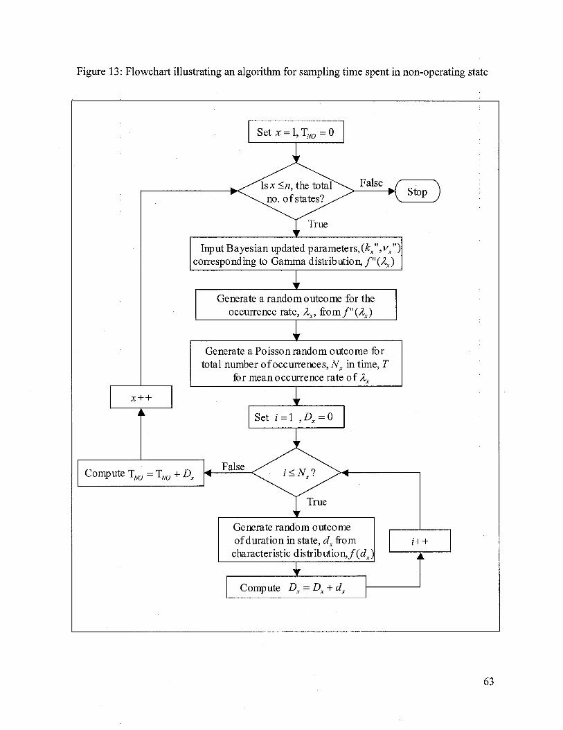
Figure 13: Flowchart illustrating an algorithm for sampling time spent in non-operating state

I

Set x = 1, TNQ =0

False

(_Stop_)

Input Bayesian updated parameters, (k”,v”)corresponding to Gamma distribution, f”(2)

Generate a random outcome for theoccurrence rate, fromf’(2)

Generate a Poisson random outcome fortotal number ofoccurrences, N in time, T

for mean occurrence rate of 2

Set i=l,D=0

True

Generate random outcomeofduration in state, d fromcharacteristic_distribution,f(d

Compute D = + d

03

PDF

Po

:T

Proc

jchc

.Dn

Tim

eof

EE

pm

IltN

c,

6161

,%

162

6163

,61

M;‘s

rvm

on

Pcr

idH

iIfy

ciir

OA

I45

0012

5

or

E-

0035

0Q

3

ou1

00

2i

00

22

5 ooI

onr’

i/

0*

II

C)

0012i

-

00

1/

CD

11

00I2

39O

iO1

430

440

4i0

44

34

491)

5(’)

510

520

530

540

Tot

alP

rxfi

wth

mT

irnc

CUni

ts:T

ric&

4y)

CD

F.P

kt;T

tP

rict

Th

nif

Eci

ipm

vnN

cg5

6I,

6162

.616

3.61

64;O

riim

Perio

d]H

iIfy

w1

1

/ /I Z

07

-I

06

51 1

-Tj

1.;

..:

.—

+

10

O4

5-

.,.....

..

.

+.

..

.

.H

.C

03

iS

0

oj

I I

42

/CD

J

011

005

I_

_—

:L

350

Y)

380

3Oi0

04i

042

030

440

5O4

470

400

490

:J0

10

520

530

540

To4i

1Pr

cDdu

ctio

nT

rnc

(Uni

ts:T

rud

dap

)

—.

-t CD

CD— 0

PDF

Pii

Toa

iPr

oduc

tion

Tim

eof

E*m

uipm

entN

o61

61.

6162

,61

61,6

164

Ob

eta

tkPe

riod

-O

rieye

ar

0.03

—i—

-—i-

——

-t-—

—i—

—-—

——

--—

——

-r-—

—r—

—-i

——

r-—

—r-

—-i

——

ufj7

5I

——

4—

__

__

0.01

115

0,01

25

0.01

0,O

t75

KO

O5

820

860

090

092

093

096

992

010

0010

2010

4010

60W

3011

00

Tt

Pri

icto

Tim

e(L

TniW

TnIc

kckL

y5)

/

/1 / /

CD

FP

ba:

Tot

alP

rod

Lion

Tim

et’E

pm

n{

Nos

.$[,

6162

,6[

63,

6164

:O

serv

aLio

riP

erio

d-

One

ye

1

0.95 09

085

07

0.65 05

C45 04 0.35 03 0.2

0.15 od 0.05

0—

800

CD CD C CD CD

CD

820

840

860

880

)00

9?.0

l060

80

1000

1020

1040

1060

1000

1100

Tot

alP

mdu

ctio

nT

ime

(1Jn

it:T

iuck-d

a

CD CD C CD

CD 00

C CD C C 0 C CD 0 C CD

AFI

9

00

l

01)1

7

kO

16

00

ê04

0012

01)1

1

0.01

eoo

0110

$

eoc

(i00

0003

o04)

PDF

P1o:

Tcd

Pro

dbci

bT

imefE

iip

mci

No

66

1,

6162

,616

3,61

64;O

icrv

aio

nPe

Hod

Two

yci

ir

w

/-

II

I

i50

1780

1800

1220

1240

180]

1880

1900

192’

]r>

01

90

1980

2000

2020

200

20

)20

8021

00

Tob

liP

roE

ctio

Tin

Tri

ck-d

ays

00

CD

FP

kLTt

aa1

Pod

uc&

nT

ime

ofE

quip

men

tN

o61

61.

6162

,61

63,

6164

,Q

iti

Pti

od

-T

oy

eCD

1

/CD

0-9-

----

---

I /-

•-

-•-

---

‘-

CDC

iC/

2

(7

._

.

-.--

-•-

•-•-

o”V

I-

-CD

06

--

.--

V--V

----

-“-.

--

-.

--

-r0

.5-----

--------

--

•-

-

--

--

----

:-g

Ij

(VA

--:..

O3

5V

:

:--

-

VV

VV

VV

VV

VV

V:V

VV

VV

VV

?V

VV

VV

0,25

-----

--

---

-V

--•---

--

u:3

/-

-_

/_‘

--

--

-—

10

.L

—t

II

ro

rso

oo

ii

io

iI3o

s3o

1900

t9*o

ic

io

2020

200

2060

2060

2100

Tota

lP

rodu

ctic

rT

rne

(Uni

ts:

Thi

ck-d

ays)

CD

PDF

Plo

tE

tono

mic

sad

Rep

sir

Cos

tsfo

rE

ilp

nw

idI4

os,

616L

6162

,61

63.

6164

;Obe

rvat

ionP

orio

dH

sify

csr

0375 035

0325 (k

3

0375

0.25

0.11

5

02

4k17

5

0.15

0125 01

00

5

0.05

0425

o -C

CD‘-

Co

(ntri

CDG

Q I-s CD (ID -t

CDcn

EL D-t

1S

22.

53

334

455

5.5

663

77,

58

Eco

ernic

and

Rqi

air

Cos

ts4%

mill

ion)

—1

C

to!H

!W$)

SOc,)

JP

dI

4JI

OU

3

Lc

vc’c

ç.

frT

Tcr

£crt

ht

zc’c

cv0

/coo

ci):

/CC

)

0

/t’O

C)

///H

)C)

/c

/.,..,,.

/—

..

..

/9

0r

/c9o

C)

./

I/

ci)/

ir/

60

/co

—_..L

II

.I_..

-1(JIH

PV

Ukj&

isq

9I9

J9

‘Zi9

I9I9

ILd

!r13

JQJS

IZ

Jb

IPU

!WcO

aW

kIicj

PDF

PbL

Eco

mic

rid

Rcpr

Cst

IbrE

quip

mcn

tNo.

6161

,66

2.

6163

, i64;

Ob

r’ti

iP

riod

Oiw

ycar

11

1

09

I-

—tI

l-J

I—

I—

ti

CD

015

OFI

0L3

0

C

CD01

C

o1 00

CD C)

006

C0

07

006

005

00

4

0

032

00

1/

01

L1

11

L1—

J_

i

335

44

56

657

75I

100

511

i15

121

2.

.31i

Ecw

iom

kn

dR

cpai

rCcts

(Sm

iflk

n)C

C

DF

Ph4:

Eco

orn

icnc

1R

qá

Ccts

fbcE

quip

rncn

tNs.

6161

,616

2.61

63,6

164:

Obcrt

ioP

crId

Onyr

______

__

__

__

__

__

__

__

__

__

t’J

11

.L

)

O9 09

(O

CDQ

/

O•9

I /I

0’

C)

O6

/1

0f-

/ I-

-CD

1.

4k5

I.

I

CD

I.

.,

..

..

‘•l

/.

..

.CD

02

CD/

..

Cl)

01

00

5 (L—

II

I

2.5

135

443

56

910

05

II11

51.2

12

13IH

1cou

cmc

nd

Rep

airC

ot

iSm

ii1io

n

Figure 24: Sampling results - PDF plot for total economic and repair costs (units: $ million)

of the four HEMM equipments in two years.

.2

/

—-

Sf_

5,

5—

I, —

Sc

0’.

Q E

____

iJLILJ—

0 0 0 0 0 0 0 0Jad

74

C

CD

FP

k’L

Ecnonic

ad

R’p

awC

os%

sft

Ehpm

eatN

45I1

M&

245

163

61&

4O

setw

LL

nP

eric

dT

ho

afs

__

__

__

____

orr

rrry

rT

Zr

1T

T]

09

-(1

)/

TI

09

//

/CD

/-

CD

07

CD

0’

/c,

O6

1

06

-°

05

/C

04%

CD0

40

O3

I

CD0

3/

/

02

o 00

1

00

Ii0

7S

910

11I

11

516

171

1921

224

I

Eco

iom

ican

dR

epar

Cosi(

mi1

ikn)

CcM

4 Discussion and Conclusions

This thesis demonstrates a novel application of structural reliability concepts for assessing

the production probabilities of ore-hauling mining operation. In particular, the thesis

contributes to the state-of-the-art in the field of mining operation productivity assessments as

follows

• Data analysis

o A novel approach for the modeling of equipment states of functioning is presented.

o Uncertainty in the occurrence rate parameter is addressed by assuming the

Poisson random occurrence model and Bayesian Inference. The utilization of

Bayesian updated distribution for estimating occurrence rate is an improvement

over the traditional technique, wherein, a point-estimate of occurrence rate is

considered. In the Bayesian updating process, the distribution of occurrence rate

becomes narrower as the number of observations (of occurrences) increase.

• Reliability analysis

o Utilization of structural reliability concepts - Limit-state-based reliability

formulations have been developed and applied for a mining application.

o The cost and production-time related reliability formulations described in the

thesis are simple to evaluate.

76

References

Ang, A.H., Tang, W.H. 2002, “Probability Concepts in Engineering: Emphasis on

Applications to Civil and Environmental Engineering”, 2nd Edition, Wiley.

Apeland, S., Scarf, P.A. 2003, “A Fully Subjective Approach to Modeling Inspection

Maintenance”, European Journal of Operational Research, v 148 n 2,p.410-25.

Benjamin, J.R., Cornell, C.A. 1970, “Probability, Statistics, and Decision for Civil

Engineers”, McGraw-Hill, New York.

Christer, A.H., Waller, W.M. 1984, “Reducing Production Downtime Using Delay-time

Analysis.”, The Journal of the Operational Research Society, v 35, p. 499—5 12.

Chung, T., Mohamed, Y., and AbouRizk, S. 2004, “Simulation Input Updating Using

Bayesian Techniques”, Proceedings of the 2004 Winter Simulation Conference.

Department of Defense Guide for Achieving Reliability, Availability, and Maintainability,

2005, Website address: http://www.acq.osd.mil/sse/docs/RAM_Guide_080305.pdf.

(Accessed - April 14, 2008)

Gupta, S., Bhattacharya, J. 1999, “Discrete Markov Chains - An Analytical Tool For

Productivity Analysis of Surface Mining Systems”, International Journal of Surface

Mining, Reclamation and Environment, v 13, n 3, p. 111-116.

Hall, R. A., Daneshmend L. K. 2003, “Reliability and Maintainability Models for Mobile

Underground Haulage Equipment”, CIMBulletin, v 96, p. 159-165.

Hall, R. A., Daneshmend L. K. 2003, “Reliability Modelling of Surface Mining Equipment:

Data Gathering and Analysis Methodologies”, International Journal of Surface

Mining, Reclamation and Environment, v 17, n 3, p. 139-155.

77

Hall, R. A., Daneshmend, L., K. 1998, “Reliability Analysis of Mobile Underground Mining

Equipment — A Case Study”, Proceedings of the 10th CIM Maintenance/Engineering

Conference, Saskatoon.

Haukaas, T., Kiureghian, A. D. 2006, “Strategies for Finding the Design Point in Non-linear

Finite Element Reliability Analysis”, Probabilistic Engineering Mechanics, v 21, n

2,p. 133-147.

Meeker Q. W., Escobar A.L. 2004, “Reliability: The Other Dimension of Quality”, Quality

Technology & Quality Management, p 1-25 (1).

Meeker Q. W., Escobar A.L. 2001, “SPLIDA (Splus Life Data Analysis): Software for

Reliability Data Analysis and Test Planning”, p. 29 (18-21).

Melchers, R. E. 1999, “Structural Reliability Analysis and Prediction (Civil Engineering)”,

2nd Edition, Wiley.

Priyadarshi, S., Hall, R.A., Streit, L., and Torjusson, G. 2006, “Maintenance and Reliability

Analysis of Haul Trucks”, Conference Proceeding.

Procaccia, H., Cordier R., and Muller S. 1997, “Application of Bayesian Statistical Decision

Theory for a Maintenance Optimization Problem”, Reliability Engineering and

System Safety, v 55, n 2, p. 143-149.

Prokopenko, V. I. 1991, Article translated from “Fiziko-Tekhnicheskie Problemy Razrabotki

Poleznykh Iskopaemykh”, v 4, p. 85-91.

Pukite, J., Pukite, P. 1998, “Modeling for Reliability Analysis: Markov Modeling for

Reliability, Maintainability, Safety, and Supportability Analyses of Complex

Computer Systems”, IEEE Press series on engineering of complex computer

problems, New York.

78

Roxana I., 2005,” Statistical Model for Estimating the Failure Probability in the Field”,

IEEE - RAMS 2005.

Sturgul, J. R. 2001, “Modeling and Simulation in Mining - Its Time Has Finally Arrived”,:

Simulation 2001, v 76, p. 286.

Vorster, M., Garza, J., 1991, “Consequential Equipment Costs Associated with Lack of

Availability and Downtime”, Journal of Construction Engineering and Management,

v 116,n4.

Yuriy, G., Vayenas, N. 2007, “Discrete-event Simulation of Mine Equipment Systems

Combined with a Reliability Assessment Model based on Genetic Algorithms”,

International Journal of Mining, Reclamation and Environment, p. 114.

79

APPENDIX A

80

A.1 Random Variable

Random variable represents an event in an analytic form. Unlike a definitive variable, the

random variable is defined within a range of possible values. For example, the random

variable, X = x,, where x e (a, b) represents an event when Xtakes on a discrete value, say x,

or a continuum of values with in a real sample set, (a, b). Random variable is denoted with

capital case letter, and the values that it can take is denoted with lower case letter.

Random variable having a countable number of possible values is a discrete random

variable. For example, if the random variable X represents the sum of two fair dices then x1

can take values ranging from 2 to 12, and the probability of X taking a discrete value 5 is as

follows

P{X = 5} = P{(1,4),(4,1),(2,3),(3,2)} =-- =--

Random variables can also take a continuum of values. For example, if the time

between failures of equipment is considered as a random variable, then the random variable

can be defined for a continuum of values say, 1.04 days, 2.2 days, 2.2 days, 45.2 days, and so

on, within a predefined sample space X= (0.1 days, 60 days) for instance. Such a random

variable is known as continuous random variable. For example, in our case, the time between

failures, t, and the mean rate of failure uA have been considered as continuous random

variables.

The uncertainty aspect of the random variable X is modeled by a probability

distribution, J(x,O). The probability distribution is a mathematical function of the values x,

that the random variable can take in its sample space and the parameter, 0, that describes the

81

distribution. For example, the time between failures of equipment t follows an exponential

distribution:

fQ,2) = -1i (Al)

The exponential distribution is a function of t the rate parameter 2. The rate parameter can

either be a point estimate, or it can be estimated using techniques like Bayesian Inference, as

will be described later. If the rate parameter is a point estimate then Eq. (1) becomes a

mathematical function of x only. However, in the Bayesian inference, the rate parameter is

also treated as a random variable.

The random variables can be assigned probability measures according to the

probability law, as discussed below.

A.2 Cumulative Distribution Function

Cumulative Distribution Function (CDF) of random variable X can be defined for any real

number x, -co< x < cy, as follows:

F(x) = P(X x)Vx (A2)

The CDF denotes the probability that the random variable X realizes a value less than or

equal to x. Similarly, the probability that.the random variable Xtakes on values which lie in

an interval (a, b).

82

The random variable X in Eq. (2) can be either discrete or continuous depending upon

whether the probability measures are defined only for discrete values of x or for all values of

x respectively.

Properties of CDF:

(a). CDF is always non-decreasing, i.e., *F(x) 0

(b). LimF(x) 0

(c). LimF(x) =1

Figure Al below illustrates a typical CDF.

Cumulative Distribution FunctionI I I I

tl)0 -

08 2 -

o -;0Q

1

0.6)

s Cumfreq

.

2

0.2 -

5 10 5 20 25 30 35 40 45 50 55

0,035, Tbf ,53.353

Time between failure

Fig. Al

A.3 Probability Mass Function

The probability distribution for a discrete random variable is described by its Probability

Mass Function (PMF). PMF expresses the probability of the random variable taking on each

of the discrete values

83

P(X x.) = p(x1)Vx1

where

(A4)

The CDF for discrete random variables is as follows

F(x1)=P(X=x)=p(x1) (A5)

A.4 Probability Density Function

For continuous random variables, the probabilities are associated with intervals of x. Further,

for any specific value ofx; only the probability density is known, i.e., P(X=x)=O

We can define the PDF as the gradient of CDF, i.e.,

= dF(x)(A6)

dx

Figure A2 below illustrates a typical PDF.

Fig. A2

84

PDF -Lognormal

ii

O.O35.

15 20 25 30 35 40 45 50 55

xl .53.353,

Time Between Failures (TBF)

A. 5 Types of Uncertainties

The uncertainties associated with data analysis are of two types: the epistemic (subjective)

uncertainty and the aleatory (inherent randomness) uncertainty. These are explained below

through examples.

1. Epistemic Uncertainty: Consider that the cost of a new engineering project at its planning

stage is to be evaluated. In order to do so, a cost function, which considers the complex

interaction of various independent variables, is developed. Some of these variables are listed

in the following.

a). Time for completion — It is influenced by the quality of schedule, level of schedule

compliance, management capabilities, etc.

b). Productivity — is influenced by the timely availability of manpower and equipments;

amount of reworks, etc.

c). External factors such as geo-political and economic environment (interest, foreign

exchange and inflation rate regimens, revenue flow profile), third party stakeholders, etc.

There exists uncertainness about the exhaustiveness of the above list. There may still

be variables which are not incorporated in the list and which influence the cost function In

such situations, the model may deviate from reality and thus the inferences drawn from the

analysis will not be realistic enough. This type of uncertainty is referred to as a model

uncertainty. Model uncertainty is an example of epistemic uncertainty, and is reflected by our

degree of belief (in the strength or, correctness of the model in this case). Epistemic

uncertainty is caused by the lack of knowledge about the factors that characterize a physical

system. Epistemic uncertainty can sometimes be reduced by further study, measurements, or

85

taking an expert opinion. The reduction of epistemic uncertainty helps in coming up with

more realistic models.

2. Aleatory Uncertainty: Consider a system comprising a set of equipments, which are

operational in an open-pit mining environment. Sudden breakdown of a part or whole of the

equipment affects the productivity of the mining operation. The breakdown may be

influenced by the occurrence of a number of chanced factors such as the amount of usage of

the equipment, quality and schedule of maintenance, operator handling, design quality,

weather conditions. The number of observed failures of the equipment within a time interval

varies randomly. Similarly, the recurrence time of failure of equipment varies with an

inherent randomness. Therefore, the uncertainty associated with the measurement of number

of failures in a time interval, or the recurrence time of failure is influenced by chance and is a

function of the system. Such uncertainty in the measurement of a variable, which is caused

by its inherent randomness, is known as an aleatory uncertainty. This uncertainty cannot be

reduced by further measurements, but can be reduced by changing the system.

A. 6 Basic Stochastic Processes

The basic stochastic processes are described in the following.

A.6.1 The Bernoulli Sequence:

An engiheering process can be modeled by random occurrence or non-occurrence of a

particular event. For example, upon inspection, a randomly chosen equipment may or may

not be defective, a new construction project may or may not get finished within its scheduled

completion time, a fair coin upon flipping may or may not yield a head, etc.

86

Consider a sequence of trials, at which the event in consideration may or may not

occur. The sequence is termed as a Bernoulli sequence, if the following conditions hold:

Only two possibilities in each trial — success or failure;

(i). Trials are statistically independent, i.e., occurrence of each trial is independent of

previous trials; and

(ii). The probability of occurrence of the event in each trial is constant, i.e., the

occurrence probability is uniform/constant over all trials.

Application of Bernoulli sequence to events occurring in time

The Bernoulli’s sequence can be applied to the random events occurring in time, by

discretizing time into various intervals (trials) and considering only two possibilities in each

interval, i.e., occurrence or non-occurrence of event. Each interval constitutes a trial and the

series of finite number of intervals constitute the Bernoulli sequence.

Therefore, if n denotes the number of intervals (each of similar duration, e.g.

days/month/year) in consideration, the random variable X represents the number of intervals

in which the event occurs, and p denotes the probability of occurrence of the event in each

respective interval. The number of occurrences then has the binomial distribution

p(x)= (n)px (1- p)flX (A7)

Mean number of occurrences = n.p

Standard deviation of number of occurrences = n.p. (l-p)

The corresponding CDF can be written as

F (x) = (I- p)’ (A8)

1=0

87

The number of intervals (trials) until an event occurs for the first time is defined by the

geometric distribution. Therefore, if ‘N’ is the random variable representing the number of

intervals before the occurrence of the specific event occurs for the first time, then

P(N = n) = p(l—p) (A9)

where n =1,2,3...

Recurrence time and return period

One important assumption in the Bernoulli sequence is the statistical independence of the

trials (time intervals in this case). If it is so then, the time interval till the first occurrence of

an event must be same as that of time between any two consecutive events. Referring to

Figure A2, the above statement implies that the time t] equals time t2. Therefore, the

probability distribution of the recurrence time is equal to that of the first occurrence time and

thus the recurrence time in a Bernoulli sequence is also governed by the geometric sequence.

T, interval size.4

occurrence 12, time period between any 2 consecutive occurrences

Start of intervals (rials,1

Time,t

II.

I

:c:ç;

ti, time elapsed until the J’ occurrence k” occurrence +1)” occurrence

Figure A2 (Illustration of the mean recurrence time in a Bernoulli sequence)

The mean recurrence time (or the return period) between two consecutive occurrences of an

event is equal to the reciprocal of the probability of the event within one time interval.

88

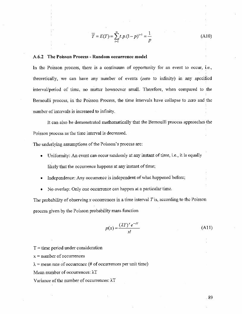
T=E(T)=t.p.(l_p)t’=1 (AlO)t=1 p

A.6.2 The Poisson Process - Random occurrence model

In the Poisson process, there is a continuum of opportunity for an event to occur, i.e.,

theoretically, we can have any number of events (zero to infinity) in any specified

interval/period of time, no matter howsoever small. Therefore, when compared to the

Bernoulli process, in the Poisson Process, the time intervals have collapse to zero and the

number of intervals is increased to infinity.

It can also be demonstrated mathematically that the Bernoulli process approaches the

Poisson process as the time interval is decreased.

The underlying assumptions of the Poisson’s process are:

• Uniformity: An event can occur randomly at any instant of time, i.e., it is equally

likely that the occurrence happens at any instant of time;

• Independence: Any occurrence is independent of what happened before;

• No overlap: Only one occurrence can happen at a particular time.

The probability of observing x occurrences in a time interval T is, according to the Poisson

process given by the Poisson probability mass function

12TX 2Te (All)x!

T time period under consideration

x = number of occurrences

= mean rate of occurrence (# of occurrences per unit time)

Mean number of occurrences:

Variance of the number of occurrences:

89

APPENDIX B

(In CD-ROM)

90