Bayesian Modelling for Matching and Alignment of

Biomolecules

P. J. Green, K. V. Mardia, V. B. Nyirongo and Y. Ruffieux

August 9, 2009

Abstract

The three-dimensional shape of a protein plays a key role in determining its function,so proteins in which particular atoms have very similar configurations in space often havesimilar functions. There is therefore a need for efficient methodology to identify, giventwo or more proteins represented by the coordinates of their atoms, subsets of thoseatoms which match within measurement error, after allowing for appropriate geometricaltransformations to align the proteins. This chapter describes a Bayesian model-basedmethodology for such tasks, and presents several challenging applications.

1 Introduction

Technological advances in molecular biology over the last 15 to 20 years have generatedmany datasets – often consisting of large volumes of data on protein or nucleotide se-quences and structure – that require new approaches to their statistical analysis. Inconsequence, some of the most active areas of research in statistics at present are aimedat such bioinformatics applications.

It is well known that proteins are the work-horses of all living systems. A protein isa sequence of amino acids, of which there are twenty types. The sequence folds into a3-dimensional structure. We can describe the shape of this structure in terms of a mainchain and side chains (for examples, see Branden and Tooze, 1999; Lesk, 2000). Threeatoms of each amino acid, denoted N , Cα and C ′, are in the main chain or backbone.The other part of the amino acid that is attached to the Cα atom is called the residue,and forms a side chain (that is, there is one side chain or residue for each amino acid inthe protein).

One of the major unsolved biological challenges is the protein folding problem: howdoes the amino acid sequence fold into a three-dimensional protein? In particular, howcan the three dimensional protein structure (and its function) be predicted from the aminoacid sequence? These are key questions, since both shape and chemistry are important inunderstanding a protein’s function.

1.1 Protein data and alignment problems

One particular task where statistical modelling and inference can contribute to scientificunderstanding of protein structure is that of matching and alignment of two or moreproteins. This chapter addresses the analysis of 3 data sets of the following nature.

1

The 3-dimensional structure of a protein is important for it to perform its function.In chemoinformatics, it is a common assumption that structurally similar molecules havesimilar activities; in consequence, protein structure similarity can be used to infer theunknown function of a candidate protein (Leach, 2003). In drug design for example, asubject of prime interest is the local interaction between a small molecule (the ligand)and a given protein receptor. If the geometrical structure of the receptor is known, thenestablished methods such as docking can be applied in order to specify the protein–ligandinteraction. However, in most cases this structure is unknown, meaning the drug designermust rely on a study of the similarity (or diversity) in available ligands.

The alignment of the molecules is an important first step towards such a study.Thus one of the problems in protein structural bioinformatics is matching and align-ing 3-dimensional protein structures or related configurations e.g. active sites, ligands,substrates, steroid molecules. To consider the matching between proteins, one normallyconsiders the Cα atoms. A related application but with different aims is the matching of2-dimensional protein gels.

Given two or more proteins represented by configurations of points in space repre-senting locations of particular atoms of the proteins, the generic task of matching andalignment is to discover subsets of these configurations that coincide, after allowing formeasurement error and unknown geometrical transformations of the proteins. These appli-cations require algorithms for matching, as well as statistics and distributions of measuresfor quantifying quality of matching and alignment.

Statistical shape analysis potentially has something to offer in solving matching andalignment problems; the field of labelled shape analysis with labelled points is well devel-oped (see Dryden and Mardia, 1998, also Appendix A.1) but unlabelled shape analysis isstill in its infancy. The methodology we have developed for matching and alignment is acontribution to shape analysis for unlabelled and partially-labelled data.

Pairwise matching of active sites data sets

An active site is a local 3-dimensional arrangement of atoms in a protein that are involvedin a specific function e.g. binding a ligand (and so known as a binding site). Atoms inactive sites are from amino acids that are close to each other in 3-dimensional space butdo not necessarily follow closely in sequence order.

We consider two datasets, analysed with different objectives. We have configura-tions of Cα atoms in two functional sites shown in Figure 1 from 17–β hydroxysteroid-dehydrogenase and carbonyl reductase proteins (two dimensional view of the data, given athttp://www.stats.bris.ac.uk/∼peter/Align/index.html). These functional sites arerelated but which and how many atoms correspond are unknown. Our aim would be tofind matching atoms and align these configurations.

We also consider matches of protein active sites from SITESDB (cf. Gold, 2003). Analcohol dehydrogenase active site (1hdx 1) is matched against NADP-binding sites of aquinone oxidoreductase protein (1qor 0); this is a small example of a query used againsta large database.

Matching multiple configurations of steroid molecules

The CoMFA (Comparative Molecular Field Analysis) database is a set of steroid moleculeswhich has become a benchmark for testing various 3D quantitative structure-activityrelationship (QSAR) methods (see Coats, 1998). This database contains the three-dimensional coordinates for the atoms in each of the 31 molecules, in addition to additional

2

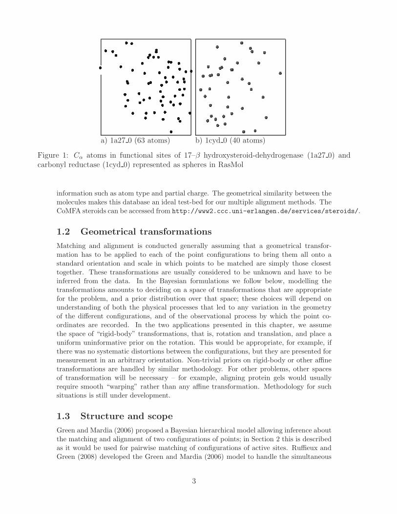
a) 1a27 0 (63 atoms) b) 1cyd 0 (40 atoms)

Figure 1: Cα atoms in functional sites of 17–β hydroxysteroid-dehydrogenase (1a27 0) andcarbonyl reductase (1cyd 0) represented as spheres in RasMol

information such as atom type and partial charge. The geometrical similarity between themolecules makes this database an ideal test-bed for our multiple alignment methods. TheCoMFA steroids can be accessed from http://www2.ccc.uni-erlangen.de/services/steroids/.

1.2 Geometrical transformations

Matching and alignment is conducted generally assuming that a geometrical transfor-mation has to be applied to each of the point configurations to bring them all onto astandard orientation and scale in which points to be matched are simply those closesttogether. These transformations are usually considered to be unknown and have to beinferred from the data. In the Bayesian formulations we follow below, modelling thetransformations amounts to deciding on a space of transformations that are appropriatefor the problem, and a prior distribution over that space; these choices will depend onunderstanding of both the physical processes that led to any variation in the geometryof the different configurations, and of the observational process by which the point co-ordinates are recorded. In the two applications presented in this chapter, we assumethe space of “rigid-body” transformations, that is, rotation and translation, and place auniform uninformative prior on the rotation. This would be appropriate, for example, ifthere was no systematic distortions between the configurations, but they are presented formeasurement in an arbitrary orientation. Non-trivial priors on rigid-body or other affinetransformations are handled by similar methodology. For other problems, other spacesof transformation will be necessary – for example, aligning protein gels would usuallyrequire smooth “warping” rather than any affine transformation. Methodology for suchsituations is still under development.

1.3 Structure and scope

Green and Mardia (2006) proposed a Bayesian hierarchical model allowing inference aboutthe matching and alignment of two configurations of points; in Section 2 this is describedas it would be used for pairwise matching of configurations of active sites. Ruffieux andGreen (2008) developed the Green and Mardia (2006) model to handle the simultaneous

3

matching of multiple configurations (see also Marın and Nieto, 2008), and this is reviewedin Section 3. Analysis of the three data sets introduced above is presented in Section 4. Weend the chapter with discussion of conclusions and future directions for research. There arevarious appendices including Appendix A.1 reviewing labelled shape analysis, AppendixB.1 on model formulation, Appendix B.2 on MCMC implementation, and Appendix B.3on web data sources.

2 A Bayesian hierarchical model for pairwise match-

ing

We have two point configurations, X(1) = {xj, j = 1, 2, . . . ,m} and X(2) = {yk, k =1, 2, . . . , n}, in d-dimensional space Rd. The points are labelled for identification, butarbitrarily. In our applications the points are Cα atoms.

A latent point process model

The key basis for our model for the configurations is that both point sets are regardedas noisy observations on subsets of a set of unobserved true locations {µi}, where we donot know the mappings from j and k to i. There may be a geometrical transformationbetween the x-space and the y-space, which may also be unknown. The objective is tomake model-based inference about these mappings, and in particular make probabilitystatements about matching: which pairs (j, k) correspond to the same true location?

We will assume the geometrical transformation between the x-space and the y-spaceto be affine, and denote it by x = Ay = Ay + τ . Later we will restrict A to be a rotationmatrix, so that this is a rigid-body transformation. We regard the true locations {µi} asbeing in x-space, without loss of generality.

The mappings between the indexing of the {µi} and that of the data {xj} and {yk}are captured by indexing arrays {ξj} and {ηk}; to be specific we assume that

xj = µξj+ ε1j , (1)

for j = 1, 2, . . . ,m, where {ε1j} have probability density f1, and

Ayk + τ = µηk+ ε2k, (2)

for k = 1, 2, . . . , n, where {ε2k} have density f2. All {ε1j} and {ε2k} are independent ofeach other, and independent of the {µi}. We take f1 and f2 to be normal but the methodgeneralises to any f1 and f2.

Multiple matches are excluded, and thus each hidden point µi is observed at mostonce in each of the x and y configurations; equivalently, the ξj are distinct, as are theηk. The label i is not used in our subsequent development, and all that is needed is thematching matrix M , defined by Mjk = 1 if ξj = ηk otherwise 0. This structure is a latentvariable in our model, and its distribution is derived from the latent point process modelas follows.

Prior for M . Suppose that the set of true locations {µi} forms a homogeneous Poissonprocess with rate λ over a region V ⊂ Rd of volume v, and that N points are realised inthis region. Some of these give rise to both x and y points, some to points of one kind andnot the other, and some are not observed at all. We suppose that these four possibilitiesoccur independently for each realised point, with probabilities parameterised so that withprobabilities (1 − px − py − ρpxpy, px, py, ρpxpy) we observe neither, x alone, y alone, or

4

both x and y, respectively. The parameter ρ is a certain measure of the tendency a priorifor points to be matched: the prior probability distribution of L conditional on m and nis proportional to

p(L) ∝ (ρ/λv)L

(m − L)!(n − L)!L!, (3)

for L = 0, 1, . . . ,min{m,n}. The normalising constant here is the reciprocal of H{m,n, ρ/(λv)},where H can be written in terms of the confluent hypergeometric function

H(m,n, d) =dm

m!(n − m)!1F1(−m,n − m + 1,−1/d),

assuming without loss of generality that n > m; (see Abramowitz and Stegun, 1970, p.504)

Assuming that M is a priori uniform conditional on L, we have

p(M) = p(L)p(M |L) =(ρ/λv)L

∑min{m,n}ℓ=0 ℓ!

(mℓ

)(nℓ

)(ρ/λv)ℓ

.

One application of this distribution of L is a similarity index (Davies et al., 2007).

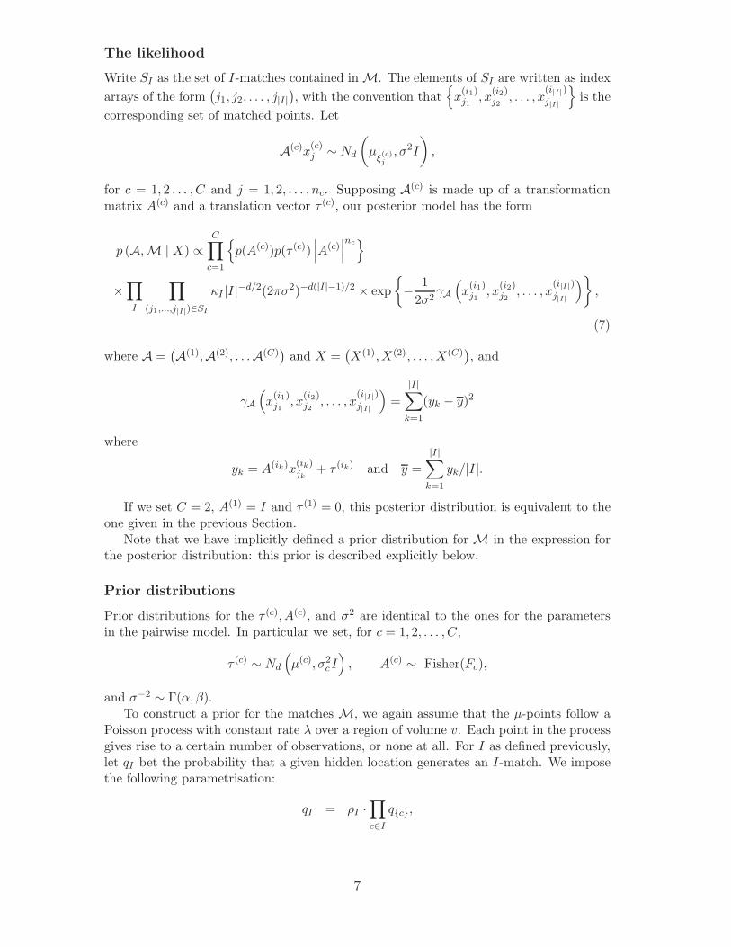
The likelihood

Letxj ∼ Nd(µξj

, σ2xI) and Ayk + τ ∼ Nd(µηk

, σ2yI),

with σx = σy = σ, say. On integrating out the µs the joint model for parameters, latentvariables and observables is (Green and Mardia, 2006)

p(M,A, τ, σ, x, y) ∝ |A|np(A)p(τ)p(σ)∏

j,k:Mjk=1

(κφ{(xj − Ayk − τ)/σ

√2}

(σ√

2)d

), (4)

where φ is the standard normal density in Rd. Here |A| is the Jacobian of transformationfrom x-space into y-space; p(A), p(τ) and p(σ) denote prior distributions for A, τ and σ;d is the dimension of the configurations i.e. d = 2 for 2-dimensional configurations e.g.protein gels and d = 3 for 3-dimensional configurations e.g. active sites; κ = ρ/λ measuresthe tendency a priori for points to be matched and can be a function of concomitantinformation e.g. amino acid types in matching protein structures. See the directed acyclicgraph, Figure 2a, for a graphical representation of the model. Green and Mardia (2006)give a generalisation where φ can be replaced by a more general density depending on f1

and f2. Details on priors are given below.There is a connection between maximising the joint posterior derived from Equation

4 and minimising root mean square deviations (RMSD), defined by

RMSD2 = Q/L, where Q =∑

j,k

Mjk||xj − Ayk − τ ||2, (5)

and L =∑

j,k:Mjk=1

Mjk denotes the number of matches. RMSD is the focus of study in

combinatorial algorithms for matching. In the Bayesian formulation the log likelihood(with uniform priors) is proportional to

const. − 2(∑

Mjk

)log σ +

(∑Mjk

)log ρ − 1

2

Q

σ2√

2.

5

The maximum likelihood estimate of σ for a given matching matrix M is the sameas the RMSD which is the least squares estimate. RMSD is a measure commonly usedin bioinformatics, although joint uncertainty in RMSD and the matrix M is difficult toappreciate except in the Bayesian formulation.

Prior distributions for continuous variables

For the continuous variables τ, σ−2 and A we use conditionally conjugate priors so

τ ∼ Nd(µτ , σ2τI), σ−2 ∼ Γ(α, β), A ∼ Fisher(F )

Here, Fisher(F ) denotes the matrix Fisher distribution; (see, for example, Mardia andJupp, 2000, p. 289). For d = 2, A has a von Mises distribution. For d = 3, it is usefulto express A in terms of the Eulerian angles. Some efficient methods to simulate A aregiven in Green and Mardia (2006). If the point configurations are presented in arbitraryorientations, it is appropriate to assume a uniform distribution on A, that is, F = 0, andthis is usually adequate.

3 Alignment of multiple configurations

In this section we consider a hierarchical model for matching configurations X(1),X(2), . . . ,X(C)

simultaneously.

Multi-Configuration Model

The pairwise model presented above can be readily extended to the multi-configurationcontext. Suppose we have C point configurations X(1),X(2), . . . ,X(C), such that X(c) ={x

(c)j , j = 1, 2, . . . , nc

}, where x

(c)j ∈ Rd and nc is the number of points in configuration

X(c). As in the pairwise case we assume the existence of a set of ‘hidden’ points µ ={µi} ⊂ Rd underlying the observations. Our multiple-configuration model is thus:

A(c)x(c)j = µ

ξ(c)j

+ ε(c)j , for j = 1, 2, . . . , nc, c = 1, 2, . . . , C. (6)

The unknown transformation A(c) brings the configuration X(c) back into the same frameas the µ-points, and ξ(c) is a labelling array linking each point in configuration X(c) toits underlying µ-point. As in the previous section the elements within each labellingarray are assumed to be distinct. In this context a match can be seen as a set of points(x

(i1)j1

, x(i2)j2

, . . . , x(ik)jk

)such that ξ

(i1)j1

= ξ(i2)j2

= . . . = ξ(ik)jk

.

Thus matches may now involve more than two points at once. These are stored in astructure M. This parameter plays the same role as the matrix M from Section 2, in thatit contains the relevant information on the matches. We choose to categorise the matchesaccording to their ‘type’. Consider a generic set I ⊂ {1, 2, . . . , C} of configuration indices,with I 6= ∅. This set corresponds to a type of match: for example if C = 3, then I = {2, 3}refers to a match involving a point from the X(2) configuration and a point from the X(3)

configuration but none from the X(1) configuration. We call I-match a match involvingexactly the configurations whose index is included in I.

6

The likelihood

Write SI as the set of I-matches contained in M. The elements of SI are written as index

arrays of the form(j1, j2, . . . , j|I|

), with the convention that

{x

(i1)j1

, x(i2)j2

, . . . , x(i|I|)

j|I|

}is the

corresponding set of matched points. Let

A(c)x(c)j ∼ Nd

(µ

ξ(c)j

, σ2I

),

for c = 1, 2 . . . , C and j = 1, 2, . . . , nc. Supposing A(c) is made up of a transformationmatrix A(c) and a translation vector τ (c), our posterior model has the form

p (A,M | X) ∝C∏

c=1

{p(A(c))p(τ (c))

∣∣∣A(c)∣∣∣nc

}

×∏

I

∏

(j1,...,j|I|)∈SI

κI |I|−d/2(2πσ2)−d(|I|−1)/2 × exp

{− 1

2σ2γA

(x

(i1)j1

, x(i2)j2

, . . . , x(i|I|)

j|I|

)},

(7)

where A =(A(1),A(2), . . .A(C)

)and X =

(X(1),X(2), . . . ,X(C)

), and

γA

(x

(i1)j1

, x(i2)j2

, . . . , x(i|I|)

j|I|

)=

|I|∑

k=1

(yk − y)2

where

yk = A(ik)x(ik)jk

+ τ (ik) and y =

|I|∑

k=1

yk/|I|.

If we set C = 2, A(1) = I and τ (1) = 0, this posterior distribution is equivalent to theone given in the previous Section.

Note that we have implicitly defined a prior distribution for M in the expression forthe posterior distribution: this prior is described explicitly below.

Prior distributions

Prior distributions for the τ (c), A(c), and σ2 are identical to the ones for the parametersin the pairwise model. In particular we set, for c = 1, 2, . . . , C,

τ (c) ∼ Nd

(µ(c), σ2

c I)

, A(c) ∼ Fisher(Fc),

and σ−2 ∼ Γ(α, β).To construct a prior for the matches M, we again assume that the µ-points follow a

Poisson process with constant rate λ over a region of volume v. Each point in the processgives rise to a certain number of observations, or none at all. For I as defined previously,let qI bet the probability that a given hidden location generates an I-match. We imposethe following parametrisation:

qI = ρI ·∏

c∈I

q{c},

7

where ρI = 1 if |I| = 1. Define LI as the number of I-matches contained in M, and assumethe conditional distribution of M given the LIs is uniform. After some combinatoricalwork we find that the prior distribution for the matches can be expressed as

p(M) ∝∏

I

( κI

v|I|−1

)LI

,

where κI = ρI/λ|I|−1. It is easy to see that this is simply a generalisation of the prior

distribution for the matching matrix M .

Identifiability issue

To preserve symmetry between configurations, we only consider the case where the A(c)

are uniformly distributed a priori. It is then true that the relative rotations(A(c1)

)′ ·A(c2)

are uniform and independent for c2 6= c1 and fixed c1. So without loss of generality, we cannow impose the identifying constraint that A(1) be fixed as the identity transformation.This is the same as saying that the first data configuration lies in the same frame as thehidden point locations, as was the case in the pairwise model.

4 Data analysis

4.1 Active sites and Bayesian refinement

4.1.1 Two sites

We now illustrate our method applying on 2 active sites described in Section 1. A sam-pler described in Appendix B.2 was run for 100,000 sweeps (including 20,000 iterationsfor burn-in period) to match 17–β hydroxysteroid-dehydrogenase and carbonyl reductaseactive sites. These sites are described in Section 1.1. Prior and hyperprior settings wereα = 1, β = 2, µτ = (0, 0, 0)′, στ = 20, λ/ρ = 0.0005, F = 0. We match 34 points asshown in Figure 3a with RMSD = 0.949A. The algorithm was also used with restric-tion to match only points representing same type of amino acid. With the restriction ontype of points (concomitant information), 15 matches shown in Figure 3b are made withRMSD = 0.727A.

4.1.2 Queries in a database

We now discuss how we could use an initial solution from other software, e.g. the graphtheoretic BK technique (Gold, 2003), derived from a physico-chemistry view point, anduse our algorithm to refine the solution. In this context, the data comparisons are substan-tial since they involve comparing a query with other family members. We compare herewith the graph theoretic approach that requires adjusting the matching distance thresholdapriori according to noise in atomic positions, which is difficult to pre-determine in bioin-formatics applications involving matching configurations in a database with varying crys-tallographic precision. Furthermore, the graph method is unable to identify alternativebut sometimes important solutions in the neighbourhood of the distance based solutionbecause of strict distance thresholds. On the other hand, the graph theoretic approach isvery fast, robust and can quickly give corresponding points for small configurations fromwhich we can get initial estimates for rotation and translation. We illustrate here how ourapproach finds more biologically interesting and statistically significant matches betweenfunctional sites (Mardia et al., 2007a).

8

a)

b)

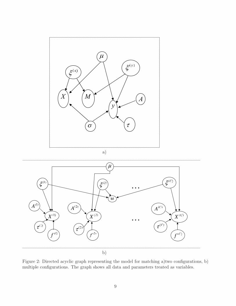
Figure 2: Directed acyclic graph representing the model for matching a)two configurations, b)multiple configurations. The graph shows all data and parameters treated as variables.

9

a) Without restriction on matches b)With restriction onmatches

Figure 3: Matched points (Cα atoms): a) without restriction on matches according to aminoacid type; b) matching rotation and same types of amino acids.

10

Figure 4: Corresponding amino acids between the NAD-binding site of alcohol dehydrogenase(1hdx 1) and NADP-binding site of quinone oxidoreductase (1qor 0) before and after MCMCrefinement step. Amino acids with bold borders are part of the dinucleotide binding motifGL-GGVG.

We model graph theoretic matches of protein active sites from SITESDB (cf. Gold,2003). An alcohol dehydrogenase active site (1hdx 1) is matched against NADP-bindingsites of a quinone oxidoreductase protein (1qor 0). Figure 4 gives matched amino acidsby the graph method and refined by the Bayesian algorithm (see Appendix B.2).

The Markov chain Monte Carlo (MCMC) refinement step produced improvementswith obvious biochemical relevance. These proteins share a well known glycine rich motif(GXGXXG) in the binding site. For 1qor 0, before the MCMC refinement step, only 2glycines in dinucleotide binding motif GLGGVG were matched by the graph theoreticapproach and this increased to 3 glycines after MCMC refinement.

In this kind of context, only short MCMC runs may be possible, and we cannot have fullconfidence that the whole posterior space is being sampled. However, we should explorethe mode containing the graph-theoretic initial solution, possibly refine that solution, andget an idea of uncertainty.

Figure 5: Superposition of matching amino acids between alcohol dehydrogenase (1hdx 1; blue)and glyceraldehyde-3-phosphate dehydrogenase (3dbv 3; red) binding sites after MCMC refine-ment (RMSD = 0.672; number of corresponding amino acids = 12; p-value = 3.68e-05). Thematched dinucleotide binding motif is shown in ball-and-stick representation. Ligands arecoloured in CPK colours.

11

4.2 Aligning multiple steroid molecules

Here we attempt to align C = 5 configurations simultaneously, using the method describedin Section 3. An MCMC algorithm (see Appendix B.2) is used to simulate a randomsample from the distribution (7); this sample is then used as a basis for inference.

We select 5 molecules from the CoMFA database (see Section 1.1); these are al-dosterone, cortisone, prednisolone, 11-deoxycorticosterone, and 17a-hydroxyprogesterone.All of these molecules contain 54 atoms. We set the following hyperparmeter values:α = 1, β = 0.1 and µ(c) = 0, σ2

c = 10, for c = 2, 3, 4, 5, and Fc = 0 for all c. For the matchprior parameters we set κI = 1 for |I| = 1, κI = 14 for |I| = 2, κI = 289 for |I| = 3,κI = 12056 for |I| = 4 and κI = 15070409 for |I| = 5. These values were determined bymaking initial ‘guesses’ on the number of matches of each type, and adapting the priordistribution (8) accordingly. As in the pairwise case we obtain estimates for the rota-tions, translations, and matches. In particular, the matches are ranked according to theirfrequency in the posterior distribution, and we choose to select the k most frequent, say.

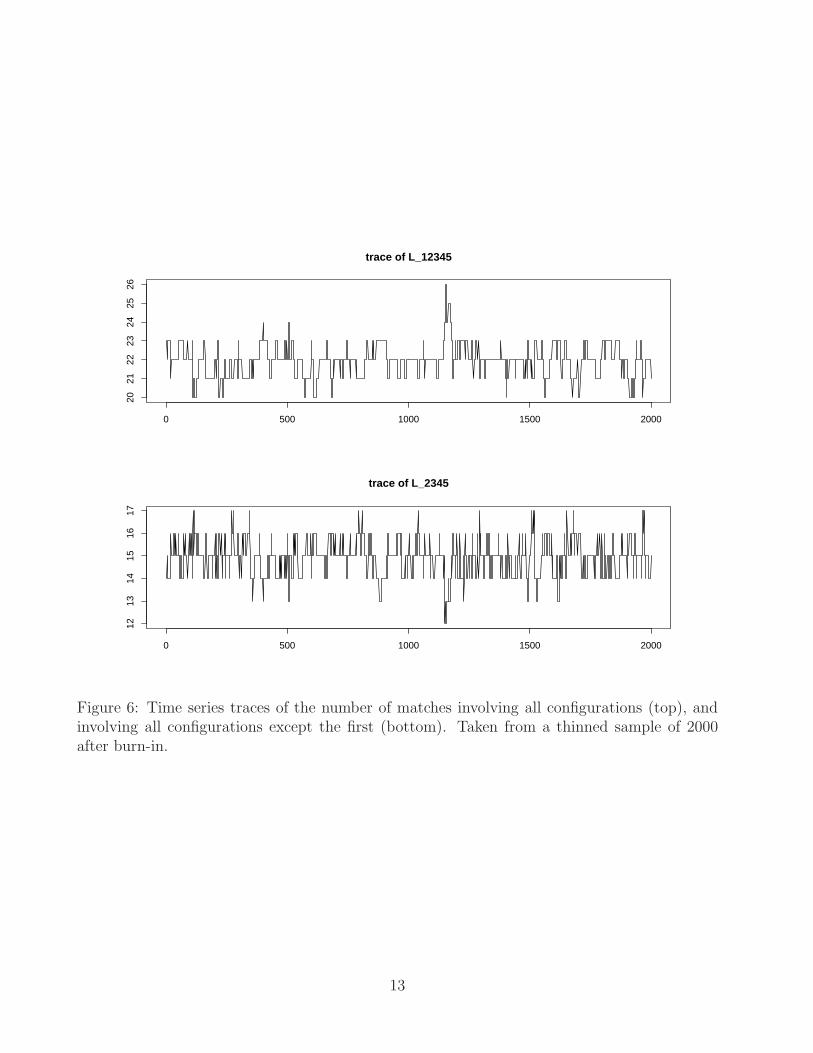
In Figure 6 we display the time series traces of L{1,2,3,4,5} and L{2,3,4,5} in the MCMCoutput. Here we find that 56 matches have sample probability higher than 0.5. In Figure7 we align the five molecules by applying the estimated transformations to each configu-ration. It is interesting to note that in the latter figure, the top right portion of the firstmolecule is slightly detached from the other four, and indeed the MCMC output suggeststhat those points from the first configuration should not be matched to the other four.However when aligning the molecules in pairs using the method from Section 2, the in-ference tends to favour matching these points, even if we set the match hyperparametersto be biased against matching. This confirms that inclusion of two or three additionalconfigurations may have a positive impact on the alignment inference. One might un-derstand this as a ‘borrowing of strength’ of sorts: further configurations provide furtherinformation on the number and location of implied µ-points, information which can inturn be exploited in the alignment of the initial configurations. Clearly there is no wayto take advantage of this information if the molecules are aligned independently in pairs.

5 Further discussion

5.1 Advantages of the Bayesian modelling approach

Some advantages of our Bayesian approach to these problems are:

1. Simultaneous inference about both discrete and continuous variables.

2. The full Bayesian posterior “tool kit” is available for inference.

3. It allows in a natural way any prior information

4. The MCMC may be too slow in some application but it has a role to play as a goldstandard against heuristic approaches.

5. The MCMC implementation provides a greater chance to escape local modes com-pared to optimisation methods.

Wilkinson (2007b) has given a review of Bayesian methods in bioinformatics and com-putational system biology more generally, citing some of these points; in particular hehas pointed out why bioinformatics and computational system biology are undergoing aBayesian revolution similar to that already seen in genetics.

12

0 500 1000 1500 2000

2021

2223

2425

26

trace of L_12345

0 500 1000 1500 2000

1213

1415

1617

trace of L_2345

Figure 6: Time series traces of the number of matches involving all configurations (top), andinvolving all configurations except the first (bottom). Taken from a thinned sample of 2000after burn-in.

13

0 2 4 6 8 10 12

−4

−2

02

4

1

11

1

11

1

1

1

1

1

1

1

1

1 1

11

1

1

1

1

1

1

1

1

1

1

1

1

11

1

1

1

1

1

1

1

1

1

1

1

1

1

1

1

1

1

1

1

1

1

1

2

22

2

22

2

2

2

2

22

2

22

2

2

2

22

2

2

22

22

2

2

2

2

2

2

2

2

2

2

2

2

2

2

2

22

2

2

2

2

2

2

2

22

2

2

3

3 3

3

33

3

3

3

3

3

3

3

3

3 3

3

33

3

3

3

3

33

3

3

3

3

3

3

3

3

33

3

3

3

3

3

3

3

3

3

3

3

3

3

3

3

33

3

3

4

44

4

44

4

4

4

4

4

4

4

4

4 4

44

4

4

4

4

4

44

4

4

4

4

4

4

4

4

4

4

4

4

4

4

4

4

4

4

4

4

4

4

44

4

4

4

4

45

55

5

55

5

5

5

5

5

5

5

5

5 5

5

55

5

5

5

5

5

5

5

5

5

5

5

5

5

5

5

5

5

5

5

5

5

5

5

5

5

5

5

5

5

5

55

5

5

5

Figure 7: Multiple alignment of the five steroid molecules: the full transformations are estimatedfrom a MCMC subsample of size 2000, and are filtered out from the data. The points areprojected onto the first two canonical axes, and are labelled according to the number of theconfiguration they belong to.

14

5.2 Outstanding issues

We expect that further work, by the authors and others, will be directed to refinement ofthe methodology described here.

5.2.1 Modelling

Spherical normality of the errors ε in (1), (2) and (6) was assumed for simplicity, andit may be necessary to relax this assumption. These errors represent both measurementerror in recording the data, and ‘model errors’, small variations between the moleculesin the locations of the atoms. There is an interplay between the sphericity assumptionand the modelling of the geometrical transformations A, so care is needed here, but it isstraightforward to replace normality by a heavy-tailed alternative.

Further study is needed on setting hyperparameters and sensitivity to these choices.The analysis seems to be most sensitive to the parameter κ but otherwise rather robust.

As mentioned before, particular applications of matching and alignment demand moresubtle modelling of the geometrical transformations A, with the extension to non-parametricwarping being most pressing.

Finally, there are interesting modelling issues concerned with using sequence informa-tion to influence the inference on matching and alignment. The most promising directionwithin our modelling paradigm involves the use of non-uniform ‘gap’ priors on the match-ing matrix M , encouraging or requiring matchings that respect the sequence order.

5.2.2 Computation

Design of MCMC samplers to deal comprehensively with problems of multimodality in theposterior distribution is the major challenge here. One can expect that generic techniquessuch as simulated tempering will have a part to play. We also expect further work oninferential methods that are perhaps not fully Bayesian, but are computationally faster,including the use of fast initialisation methods, such as

(a) Starting from the solution from 3-dimensional deterministic methods such as graphtheoretic, CE, geometric hashing and others.

(b) For full protein alignment of structure, using well established sequence alignmentsoftware e.g. BLAST as the starting point.

5.3 Alternative approaches

5.3.1 EM approach

The interplay between matching (that is, allocation), and parameter uncertainty has some-thing in common with mixture estimation. This might suggest considering maximisationof the posterior by using the EM algorithm, which could of course in principle be appliedeither to maximum likelihood estimation or to maximum a posteriori estimation. For theEM formulation, the “missing data” are the matches.

The “expectations of missing values” are just probabilities of matching. These areonly tractable if we drop the assumption that a point can only be matched with at mostone other point; that is, that

∑j Mjk ≤ 1 for all k,

∑k Mjk ≤ 1 for all j. We then get

“soft matching”.EM allows us to study only certain aspects of an approximate version of our model,

and is not trivial numerically. Obtaining the complete posterior by Markov chain Monte

15

Carlo sampling gives much greater freedom in inference. For a direct EM approach seeKent et al. (2004, 2008).

5.3.2 Procrustes type approaches

Dryden et al. (2007) and Schmidler (2007) use a MAP estimator for M after estimating“nuisance parameters” (A, τ , σ2) from Procrustes registration. Schmidler (2007) has pro-vided a fast algorithm using geometric hashing. Thus these borrow strength from labelledshape analysis. The Green and Mardia (2006) procedure also allows informative priorsso the procedure is very general. Dryden (2007) has given some initial comparisons andin particular their MAP approach often get stuck in local modes. For small variability,both approaches lead to similar results. Wilkinson (2007a) has touched many importantproblems in Bayesian alignment in particular the uniform prior would be strongly biasedtowards larger values of L = |M |. Schmidler (2007) and Dryden et al. (2007) effectivelyassume that Procrustes alignment is “correct” and does not reflect uncertainty in geo-metric alignment. By integrating out the geometrical transformation as in Green andMardia (2006) then alignment uncertainty will be propagated correctly without sufferingsignificant computation penalty. Mardia (2007a) has raised a few general issues aboutmatching in the discussion.

5.4 Future directions

Bayesian approaches are particularly promising in tackling problems in bioinformatics,with their inherent statistical problems of multiple testing, large parameter spaces foroptimisation and model or parameter non-identifiability due to high dimensionality. Oneof the major statistical tasks is to build simulation models of realistic proteins by incorpo-rating local and long-range interactions between amino acids. A protein can be uniquelydetermined by a set of conformational angles so directional statistics (see Mardia andJupp, 2000) plays a key role as well as shape analysis. Boomsma et al. (2008) has givena dynamical Bayesian network with angular distributions and amino acid sequences asits nodes for protein (local) structure prediction. This solves one of the two major bottlenecks for protein based nanotechnology namely generating native(natural) protein-likestructures. Another is an appropriate energy function to make it compact. The angulardistributions used a priori adequately describe Ramachandran plots of the dihedral an-gles of the backbone (see Mardia, Taylor and Subramaniam, 2007b; Mardia et al., 2008).Hamelryck et al. (2006) have given a method of simulating realistic protein conformationfor Cα trace focusing on mimicking secondary structure while Mardia and Nyirongo (2008)focus on global properties e.g. compactness and globularity.

The word homology is used in a technical sense in biology, especially in discussionof protein sequences, which are said to be homologous if they have been derived from acommon ancestor. Homology implies an evolutionary relationship and is distinct fromsimilarity. In this chapter, alignment focuses only on similarity.

To sum up, there are real challenges for statisticians in the understanding of proteinstructure. Similar remarks apply to understand the RNA structure (see, for exampleFrellsen et al., 2008). All this might need is holistic statistics which implies a shift ofparadigm by statisticians (Green, 2003; Mardia and Gilks, 2005; Mardia, 2007b, 2008).However, protein bioinformatics is a subset of very large area of bioinformatics which hasmany challenging problems (see Gilks, 2004; Mardia, 2005; Wilkinson, 2007b).

16

Acknowledgements

V.B. Nyirongo acknowledges funding from the School of Mathematics, University of Leedsas a visiting research fellow during the period in which part of this chapter was drafted.

References

Abramowitz, M. and Stegun, I.A. (1970), Handbook of Mathematical Functions, Dover,New York.Artymiuk, P.J., Poirrette, A.R., Grindley, H.M., Rice, D.W. and Willett, P. (1994), Agraph-theoretic approach to the identification of three-dimensional patterns of aminoacid side-chains in protein structures, J. Mol. Biol. 243, 327–44.

Berkelaar, M. (1996), lpsolve - simplex-based code for linear and integer programming,http://www.cs.sunysb.edu/~algorith/implement/lpsolve/implement.shtml.

Bookstein, F.L. (1986). Size and shape spaces for landmark data in two dimensions.Statistical Science, 1, 181-242.

Boomsma, W., Mardia, K.V., Taylor, C.C., Perkinghoff-Borg, J., Krogh, A. and Hamel-ryck, T. (2008), A generative, probabilistic model of local protein structure, Proceedings

of the National Academy of Science 105, 8932–8937.

Branden, C. and Tooze, J. (1999), Introduction to Protein Structure, 2nd edition, GarlandPublishing Inc, New York.

Burkard, R.E. and Cela, E. (1999), Linear assignment problems and extensions, in

P. Pardalos and D.-Z. Du, eds, Handbook of Combinatorial Optimization, Vol. 4, 75–149, Kluwer Academic Press, Boston.

Coats, E.A. (1998), The CoMFA steroid database as a benchmark dataset for developmentof 3D QSAR methods, Perspectives in Drug Discovery and Design 12-14, 199–213.

Davies, J.R., Jackson, R.M., Mardia, K.V. and Taylor, C.C. (2007), The Poisson index:A new probabilistic model for protein-ligand binding site similarity, Bioinformatics

23, 3001–3008.

Dryden, I.L. (2007), Discussion to Schmidler, 17–18. Listed here.

Dryden, I.L., Hirst, J.D. and Melville, J.L. (2007), Statistical analysis of unlabelled pointsets: comparing molecules in chemoinformatics, Biometrics 63, 237251.

Dryden, I.L. and Mardia, K.V. (1998), Statistical Shape Analysis, John Wiley, Chichester.

Frellsen, J., Moltke, I., Thiim, M., Mardia, K.V., Ferkinghoff-Borg, J. and Hamelryck, T.(2008), A probabilistic model of local RNA 3-d structure, Submitted.

Gilks, W. (2004), Bioinformatics: new science- new statistics., Significance 1, 7–9.

Gold, N.D. (2003), Computational approaches to similarity searching in a functional sitedatabase for protein function prediction, Ph.D thesis, Leeds University, School of Bio-chemistry and Microbiology.

Green, P.J. (2003), Diversities of gifts, but the same spirit., The Statistician 52, 423-438.

17

Green, P.J. and Mardia, K.V. (2006), Bayesian alignment using hierarchical models, withapplications in protein bioinformatics, Biometrika 93(2), 235–254.

Hamelryck, T., Kent, J.T. and Krogh, A. (2006), Sampling realistic protein conformationsusing local structural bias, Computational Biology 2(9), 1121–1133.

Holm, L. and Sander, C. (1993), Protein structure comparison by alignment of distancematrices, J. Mol. Biol. 233, 123–138.

Horgan, G.W., Creasey, A. and Fenton, B. (1992), Superimposing two dimensional gelsto study genetic variation in malaria parasites, Electrophoresis 13, 871–875.

Jonker, R. and Volgenant, A.A. (1987), Shortest augmenting path algorithm for denseand spare-linear assignment problems, Computing 38, 325–340.

Kendall, D.G. (1984). Shape manifolds, Procrustean metrics and complex projectiveshapes. Bulletin of London Mathematical Society, 16, 81–121.

Kent, J.T. (1994). The complex Bingham distribution and shape analysis. Journal of the

Royal Statistical Society, Series B, 56, 285-299.

Kent, J.T., Mardia, K.V. and Taylor, C.C. (2004), Matching problems for unlabelledconfigurations, in R. Aykroyd, S. Barber and K. Mardia, eds, Bioinformatics, Images,and Wavelets, Leeds University Press, 33–36.

Kent, J.T., Mardia, K.V. and Taylor, C.C. (2008), Bioinformatics and the problem ofmatching unlabelled configurations, Submitted.

Le, H.L. (1988). Shape theory in flat and curved spaces, and shape densities with uniform

generators. Ph.D. thesis, University of Cambridge.

Leach, A.R. and Gillet, V.J. (2003), An Introduction to Chemoinformatics, Kluwer Aca-demic Press, London.

Lesk, A.M. (2000), Introduction to protein architecture, Oxford University Press, Oxford.

Mardia, K.V. (2005), A vision of statistical bioinformatics, in S. Barber, P.D. Baxter,K.V. Mardia and R.E. Walls, eds, LASR2005 Proceedings, Leeds University Press, 9–20.

Mardia, K.V. (2007a), Discussion to Schmidler, 18. Listed here.

Mardia, K.V. (2007b), On some recent advancements in applied shape analysis and direc-tional statistics, in S. Barber, P.D. Baxter and K.V. Mardia, eds, Systems Biology &Statistical Bioinformatics, Leeds University Press, 9–17.

Mardia, K.V. (2008), Holistic statistics and contemporary life sciences, in LASR Proceed-ings, Leeds University Press, 9–17.

Mardia, K.V. and Gilks, W. (2005), Meeting the statistical needs of 21st-century science,Significance 2, 162–165.

Mardia, K.V., Hughes, G., Taylor, C.C. and Singh, H. (2008), Multivariate von misesdistribution with applications to bioinformatics, Canadian Journal of Statistics 36, 99–109.

18

Mardia, K.V. and Nyirongo, V.B. (2008), Simulating virtual protein Cα traces with ap-plications, J. Comp. Biology 15(9), 1221–1236.

Mardia, K.V. and Jupp, P.E. (2000), Directional Statistics, John Wiley and Sons Ltd,Chichester.

Mardia, K.V., Nyirongo, V.B., Green, P.J., Gold, N.D. and Westhead, D.R. (2007a),Bayesian refinement of protein functional site matching, BMC Bioinformatics 257.

Mardia, K.V., Taylor, C.C. and Subramaniam, G.K. (2007b), Protein bioinformatics andmixtures of bivariate von mises distributions for angular data, Biometrics 63, 505–512.

Marın, J.M. and Nieto, C. (2008), Spatial Matching of Multiple Configurations of Pointswith a Bioinformatics Application, Communications in Statistics - Theory and Methods

37(12), 1977–1995.

Ruffieux, Y. and Green, P.J. (2008), Alignment of multiple configurations using hierar-chical models. To appear in Journal of Computational and Graphical Statistics.Available at http://www.stats.bris.ac.uk/~peter/papers/MAlign.pdf.

Schmidler, S.C. (2007), Fast Bayesian shape matching using geometric algorithms, in

J. Bernardo, M. Bayarri, J. Berger, A. Dawid, D. Heckerman, A. Smith and W. M.,eds, Bayesian Statistics, Oxford University Press, 1–20.

Wilkinson, D.J. (2007a), Discussion to Schmidler (2007), 13–17.

Wilkinson, D.J. (2007b), Bayesian methods in bioinformatics and computational systemsbiology, Briefings in Bioinformatics 8(2), 109–116.

19

Appendix A.1 Broader context and background

Shape Analysis

Advances in data acquisition technology have led to the routine collection of geometricalinformation, and the study of the shape of objects has been increasingly important. Withmodern technology, locating points on objects is now often straightforward. Such points,typically on the outline or surface of the objects, can be loosely described as landmarks,and in this discussion, and indeed throughout the chapter, we treat objects as beingrepresented by their landmarks, regarded as points in a euclidean space, usually R2 orR3.

What do we mean by ‘shape’? The word is very commonly used in everyday language,usually referring to the appearance of an object. Mathematically, shape is all the geo-metrical information that remains when certain transformations are filtered out, that is,a point in shape space represents an equivalence class of objects, equivalent under trans-formations of the given kind. We are typically concerned with transformations such astranslation and rotation, sometimes with uniform scale change and/or reflection, and lesscommonly with unequal scale change, and hence affine transformation, or even non-affinetransformations such as non-parametric warping.

When we use the term rigid shape analysis we refer to the most important case inapplications to bioinformatics, where the transformations in question are translationsand rotations, that is, rigid-body motions. This case might more formally be termedsize and shape analysis, or the analysis of form. The more common notion of shape inmorphometrics is similarity shape, where uniform scale change is also allowed. In reflection

shape analysis, the equivalence class also allows reflections.To visualise the distinctions, consider right-angled triangles △ABC with sides in the

ratio AB : BC : CA = 3 : 4 : 5. In reflection shape space, all such triangles are equivalent.For equivalence in similarity shape space, their vertices must be ordered in the same sense(clockwise or anticlockwise), and in rigid shape space, they must also have the same size.

Most theory and practice to date is concerned with the case of labelled shape analysis,where the landmarks defining an object are uniquely identified, so are regarded mathe-matically as an ordered set (or stacked as a matrix). But increasingly we see applications,including that dealt with in the present chapter, in which the landmarks are either notidentified at all (the unlabelled case) or identification is incomplete, so that two differentlandmarks can have the same label (which we might call the partially labelled case). Inthe unlabelled case, the landmarks form an unordered set. To return to our 3:4:5 triangle,in unlabelled rigid shape analysis, the triangles with AB = 3, BC = 4, CA = 5 and withAB = 4, BC = 5, CA = 3 are equivalent, because for example the vertices identified withA in the two figures are not associated.

The foundation for similarity space analysis was laid by Kendall (1984). For mathe-matical representation, we can construct a shape space with an appropriate metric. Themetric is a Procrustes distance for the Kendall shape space. For the form space (see Le,1988) the appropriate distance is the RMSD (equation (4)). Note that in practice spe-cific coordinate representations of shape have been useful, namely Bookstein coordinates(Bookstein, 1986) and Procrustes tangent coordinates (Kent, 1994). For further details,see for example, Dryden and Mardia (1998).

Alignment and matching problems such as those considered in this chapter extendunlabelled and partially-labelled shape analysis to embrace settings where the point con-figurations are supersets of those that can be matched, so that the analysis includes anelement of selection of points to be matched as well as inference about the geometrical

20

transforations involved.

Appendix B.1 Model Formulation and Inference

Pairwise Model

Using concomitant information

When the points in each configuration are ‘coloured’, with the interpretation that like-coloured points are more likely to be matched than unlike-coloured ones, it is appropriateto use a modified likelihood that allows us to exploit such information. Let the coloursfor the x and y points be {rx

j , j = 1, 2, . . . ,m} and {ryk , k = 1, 2, . . . , n} respectively. The

hidden-point model is augmented to generate the point colours, as follows. Independentlyfor each hidden point, with probability (1 − px − py − ρpxpy) we observe neither x nor ypoint, as before. With probabilities pxπ

xr and pyπ

yr , respectively, we observe only an x or

y point, with colour r from an appropriate finite set. With probability

ρpxpyπxr πy

s exp(γI[r = s] + δI[r 6= s]),

where I[·] is an indicator function, we observe an x point coloured r and a y point coloureds. Our original likelihood is equivalent to the case γ = δ = 0, where colours are inde-pendent and so carry no information about matching. If γ and δ increase, then matchesare more probable, a posteriori, and, if γ > δ, matches between like-coloured points aremore likely than those between unlike-coloured ones. The case δ → −∞ allows the pro-hibition of matches between unlike-coloured points, a feature that might be adapted toother contexts such as the matching of shapes with given landmarks.

In implementation of this modified likelihood, the Markov chain Monte Carlo accep-tance ratios derived for M can be easily modified.

Other, more complicated, colouring distributions where the log probability can beexpressed linearly in entries of M can be handled similarly.

Continuous concomitant information can be incorporated in our statistical modelssuch as incorporating van der Waal radii. Such models will be very similar in characteras above with obvious modifications e.g. by using pairwise interaction potentials insteadof indicator functions.

Loss functions and a point estimate of M

The output from the Markov chain Monte Carlo sampler derived above, once equilibrated,is a sample from the posterior distribution. As always with sample-based computation,this provides an extremely flexible basis for reporting aspects of the full joint posteriorthat are of interest.

We consider loss functions L(M,M) that penalise different kinds of error and do socumulatively. The simplest of these are additive over pairs (j, k). Suppose that the loss

when Mjk = a and Mjk = b, for a, b = 0, 1, is ℓab; we set ℓ00 = ℓ11 = 0. For example, ℓ01

is the loss associated with declaring a match between xj and yk when there is really none,that is, a ‘false positive’. Then

E{L(M,M )|x, y} = −(ℓ10 + ℓ01)∑

j,k: Mjk=1

(pjk − K),

whereK = ℓ01/(ℓ10 + ℓ01),

21

and pjk = pr(Mjk = 1|x, y) is the posterior probability that (j, k) is a match, whichis estimated from a Markov chain Monte Carlo run by the empirical frequency of thismatch. Thus, provided that ℓ10 + ℓ01 > 0 and ℓ01 > 0, as is natural, the optimal estimateis that maximising the sum of marginal posterior probabilities of the declared matches∑

j,k: Mjk=1pjk, penalised by a multiple K times the number of matches. The optimal

match therefore depends only through the cost ratio K. If false positive and false negativematches are equally undesirable, one can simply choose K = 0.5.

Computation of the optimal match M would be trivial but for the constraint that therecan be at most one positive entry in each row and column of the array. This weightedbipartite matching problem is equivalent to a mathematical programming assignmentproblem, and can be solved by special-purpose or general LP methods; (see Burkard andCela, 1999).

For problems of modest size, the optimal match can be found by informal heuristicmethods. These may not even be necessary, especially if K is not too small. In particular,it is immediate that, if the set of all (j, k) pairs for which pjk > K includes no duplicated

j or k value, the optimal M consists of precisely these pairs. For aligning large size ofprotein chains lpSolve needs to be replaced by linearass (Jonker and Volgenant, 1987).

Appendix B.2 Model Implementation

Sampling the posterior distribution for pairwise alignment

It is straightforward to update conditionally continuous variables. For updating M con-ditionally, we need some new ways.

The matching matrix M is updated in detailed balance using Metropolis-Hastingsmoves that only propose changes to a few entries: the number of matches L =

∑j,k Mjk

can only increase or decrease by 1 at a time, or stay the same. The possible changes areas follows:

(a) adding a match, which changes one entry Mjk from 0 to 1;

(b) deleting a match, which changes one entry Mjk from 1 to 0;

(c) switching a match, which simultaneously changes one entry from 0 to 1 and anotherin the same row or column from 1 to 0.

The proposal proceeds as follows. First a uniform random choice is made from all them+n data points x1, x2, . . . , xm, y1, y2, . . . , yn. Suppose without loss of generality, by thesymmetry of the set-up, that an x is chosen, say xj . There are two possibilities: either xj

is currently matched, in that there is some k such that Mjk = 1, or not, in that there isno such k. This depends on p⋆; if xj is matched to yk, with probability p⋆ it is proposeddeleting the match, and with probability 1 − p⋆ we propose switching it from yk to yk′ ,where k′ is drawn uniformly at random from the currently unmatched y points. On theother hand, if xj is not currently matched, it is proposed adding a match between xj anda yk, where again k is drawn uniformly at random from the currently unmatched y points.

The acceptance probabilities for these three possibilities are easily derived (see Greenand Mardia, 2006)

Note that this procedure bypasses the reversible jump.

Multimodality

The issue of multimodality is a challenging issue, as we point out in Green and Mardia(2006). The MCMC samplers used here are very simple (but adequate for the presented

22

examples), and there is a vast literature on more powerful methods that we have not yetbrought to bear; this is one of the areas that needs exploring. See also discussion byWilkinson (2007a).

Sampling the posterior distribution for multiple alignment

With our conditionally conjugate priors, we can update the parameters τ (c), A(c), and σ2

using a Gibbs move, as in the pairwise implementation. Generalising the updating of thematches to the multi-configuration context is less obvious. Write

M ={(

t11, t12, . . . , t

1C

),(t21, t

22, . . . , t

2C

), . . . ,

(tK1 , tK2 , . . . , tKC

)}.

Each C-tuple (tk1 , tk2 . . . , tkC) represents a match, tkc being the index of the point from

the x(c) configuration involved in the match. If a given configuration is not involved inthe match, a ‘−’ flag is inserted at the appropriate position. For instance, if C = 3 the

3-tuple (2, 4, 1) refers to a match between x(1)2 , x

(2)4 and x

(3)1 , while (−, 2, 1) is a match

between x(2)2 and x

(3)1 , with no x(1)–point involved. We also include unmatched points in

this list: (1,−,−) indicates that x(1)1 is unmatched, for example.

Suppose that M is the current list of matches in the MCMC algorithm. We define ajump proposal proceeds as follows:

• with probability q we choose to split a C-tuple; in this case we draw an elementuniformly at random in the list M.

– If the C-tuple drawn corresponds to an unmatched point, we do nothing;

– otherwise we split it into two C-tuples at random; for instance (2, 3, 1) can besplit into (2,−,−) and (−, 3, 1).

• With probability 1 − q we choose to merge two C-tuples; in this case we select twodistinct elements uniformly at random from M.

– If the two C-tuples drawn contain a common configuration, e.g. (j1, k,−) and(j2,−,−), then we do nothing;

– otherwise we merge the C-tuples, for example (j, k,−) and (−,−, l) become(j, k, l), while (−, k,−) and (−,−, l) become (−, k, l).

This defines a Metropolis-Hastings jump, and its acceptance probability can be readilyworked out from (7).

23

Appendix B.3 Other Data Sources

• PDB databank: This is a web resource for protein structure data (http://www.rcsb.org/pdb/).The RCSB PDB also provides a variety of tools and resources for studying struc-tures of biological macromolecules and their relationship to sequence, function anddisease.

– PDBsum is a value added tool for understanding protein structure. Another im-portant tool is SWISS-MODEL server which uses HMM for homology modellingto identify structural homologs of a protein sequence.

– There are also tools for displaying 3-dimensional structures e.g. RasMol, JMol,KiNG, WebMol, MBT SimpleView, MBT Protein Workshop and QuickPDB(JMol is a new version of RasMol but is JAVA based).

• SitesBase: Resource for data on active sites. The database holds pre-compiled in-formation about structural similarities between known ligand binding sites found inthe Protein Data Bank. These similarities can be analysed in molecular recognitionapplications and protein structure-function relationships.http://www.bioinformatics.leeds.ac.uk/sb.

• NPACI/NBCR resource: A database and tools for 3-dimensional protein structurecomparison and alignment using the Combinatorial Extension (CE) algorithm.http://cl.sdsc.edu/ce.html.

• The Dali Database: This database is based on exhaustive, all-against-all 3-dimensionalstructure comparison of protein structures in the Protein Data Bank. Alignmentsare automatically maintained and regularly updated using the Dali search engine.http://ekhidna.biocenter.helsinki.fi/dali server/

• SCOP: Aims to provide a detailed and comprehensive description of the structuraland evolutionary relationships between all proteins whose structure is known. Assuch, it provides a broad survey of all known protein folds, detailed information aboutthe close relatives of any particular protein, and a framework for future research andclassification.http://scop.mrc-lmb.cam.ac.uk/scop/

• CATH: Describes the gross orientation of secondary structures, independent of con-nectivities and is assigned manually. The topology level clusters structures into foldgroups according to their topological connections and numbers of secondary struc-tures. The homologous superfamilies cluster proteins with highly similar structuresand functions. The assignments of structures to fold groups and homologous super-families are made by sequence and structure comparisons. http://www.cathdb.info/

• BLAST: Basic Local Alignment Search Tool, or BLAST, is an algorithm for com-paring primary biological sequence information, such as the amino-acid sequences ofdifferent proteins. A BLAST search enables a researcher to compare a query sequencewith a library or database of sequences, and identify library sequences that resemblethe query sequence above a certain threshold. http://blast.ncbi.nlm.nih.gov/Blast.cgi

24