Bayesian estimation in IRT models with missing values in ... · Bayesian estimation in IRT models with missing values in background variables 597 approach is a two-step approach that

Psychological Test and Assessment Modeling, Volume 57, 2015 (4), 595-618

Bayesian estimation in IRT models with missing values in background variables

Christian Aßmann1, Christoph Gaasch2, Steffi Pohl3 & Claus H. Carstensen2

Abstract

Large scale assessment studies typically aim at investigating the relationship between persons competencies and explaining variables. Individual competencies are often estimated by explicitly including explaining background variables into corresponding Item Response Theory models. Since missing values in background variables inevitably occur, strategies to handle the uncertainty related to missing values in parameter estimation are required. We propose to adapt a Bayesian estimation strategy based on Markov Chain Monte Carlo techniques. Sampling from the posterior distribution of parameters is thereby enriched by sampling from the full conditional distribution of the missing values. We consider non-parametric as well as parametric approximations for the full conditional distributions of missing values, thus allowing for a flexible incorporation of metric as well as cate-gorical background variables. We evaluate the validity of our approach with respect to statistical accuracy by a simulation study controlling the missing values generating mechanism. We show that the proposed Bayesian strategy allows for effective comparison of nested model specifications via gauging highest posterior density intervals of all involved model parameters. An illustration of the suggested approach uses data from the National Educational Panel Study on mathematical compe-tencies of fifth grade students.

Keywords: missing values, background variables, classification and regression trees, item response theory

1 Correspondence concerning this article should be addressed to: Dr. Christian Aßmann, Otto-Friedrich-University Bamberg, Feldkirchenstr. 21, 96045 Bamberg, Germany; email: [email protected] 2 Leibniz Institute for Educational Trajectories Bamberg, Germany; Otto-Friedrich-Universität Bamberg, Germany 3 Free University Berlin, Germany

C. Aßmann, C. Gaasch, S. Pohl & C. H. Carstensen 596

1 Introduction

With large scale assessments, such as the Program for International Student Assessment (PISA; e.g., OECD, 2012), the Third International Mathematics and Science Study (TIMSS; e.g., Mullis, Martin, Foy, & Arora, 2012), the National Assessment of Educa-tional Progress in the United States (NAEP; e.g., National Center for Education Statis-tics, 2013) or the German National Educational Panel Study (NEPS; e.g., Blossfeld, Roßnach, & Maurice, 2011), researchers aim at investigating the relationship between competencies and explaining variables. Typical research questions concern, for example, the explanation of competencies and competence development based on individual char-acteristics like gender, socio-economic status, migration background, and context varia-bles like school characteristics. Competencies in large scale studies are assessed via tests (see e.g. OECD, 2012; Weinert, et al., 2011) and competence data are usually analyzed via Item Response Theory (IRT) models. IRT models belong to the group of Confirmato-ry Item Factor Analysis (CIFA) models (see Edwards, 2010). These models include, for example, the Rasch model (Rasch, 1960), the Partial Credit model (Masters, 1982), the 3-parameter logistic model (Birnbaum, 1968), or the corresponding model counterparts based on the normal ogive description (see, e.g., Albert, 1992; Béguin & Glas, 2001). All these modeling approaches have in common that parameter estimation within these frameworks routinely relies on the Likelihood principle either in form of Maximum Likelihood (ML) estimation typically performed via the EM-algorithm, or in form of Bayesian approaches using Markov Chain Monte Carlo (MCMC) based techniques (see Edwards, 2010). Since the derived likelihood functions or moment equations involve high-dimensional integrals or incorporate latent structures, the considered model frame-works are in principle straightforward to handle within a Bayesian estimation approach using MCMC techniques. Further, all these different modeling frameworks offer the possibility to be extended to incorporate auxiliary information in form of context (back-ground) variables of the examinees into the estimation of ability parameters (Mislevy, 1987). Incorporating auxiliary information in form of context variables enhances effi-ciency of estimates and allows for direct assessment of dependencies between the latent abilities and context variables.

Despite tremendous efforts in field work, missing values in these background variables occur. Usually these missing values are treated via multiple imputation (Rubin, 1987) including relevant variables in the imputation model to capture dependencies. Specifical-ly questionnaire variables (i.e., background variables) are needed for the provision of competence scores (in form of plausible values) and questionnaire variables as well as latent competence scores are needed for the imputation of missing responses in question-naire items. Other large scale studies, such as PISA and NAEP, deal with this problem by using missing indicators for each questionnaire variable (indicating whether the re-sponse on this variable is observed or missing) and aggregating the questionnaire varia-bles and the response indicators to orthogonal factors. The set of factors is then used as background variables in the IRT measurement model of the competence data (see Allen, Carlson, Johnson & Mislevy, 2001). Thereby, as many factors as needed to explain 90 percent of the variance of the questionnaire items are typically considered. However, this

Bayesian estimation in IRT models with missing values in background variables 597

approach is a two-step approach that does not incorporate the latent competence score in the imputation of the questionnaire variables and does not depict the uncertainty stem-ming from missing values in questionnaire items.

We propose to extend available Bayesian estimation routines relying on MCMC meth-odology and augment the parameter vector with the missing values in the background variables. The advantages of the suggested approach compared to a two-step approach relate to increased statistical efficiency and model consistency. Whilst the current model presupposes the distribution of latent abilities to depend on background variables, this dependence could not be reflected to the full extent by a two-step approach using some pre estimated latent ability for the imputation of background variables. Fully accounting for the assumed conditional variables further increases the statistical accuracy in terms of efficiency in assessing the influence of background variables competencies. As the back-ground variables are not subject to specific modelling, flexible ad hoc assumptions are required to provide a valid approximation of the underlying full conditional distribution of the missing values. While parametric normal models, as used in Aßmann, Gaasch, Pohl, & Carstensen (2016), offer flexible handling of missing values in metric back-ground variables, background variables in large-scale assessments are typically also categorically scaled. Hence, in this paper we suggest to adapt non-parametric approxima-tions to the full conditional distributions based on sequential regression trees. As dis-cussed within the literature (Burgette & Reiter, 2010; Doove, van Buuren, & Dusseldorp, 2014), these are also able to model more complex dependencies, for example, higher order interactions. The MCMC approach allows furthermore for direct assessment of accuracy measures of estimators without requirement to use combining rules typically needed when analyzing data sets with missing values.

In the following we will first describe the IRT framework and the Bayesian estimation routines used in our approach. We will then present our hybrid sampling scheme and demonstrate its performance first in a simulation study investigating the estimation accu-racy and second by an empirical example demonstrating the applicability of the ap-proach.

2 Item Response Theory for scaling of competence tests

In large scale assessments often different competence domains are assessed, for example reading, mathematical competence, science, and computing literacy. The competence domains are assessed by tests that contain a number of items that may be dichotomously or polytomously scored. Different types of IRT models are used in the different large scale assessment studies. While PISA (OECD, 2012) and NEPS (Pohl & Carstensen, 2012) rely on one parameter IRT models such as the Rasch model (Rasch, 1960) or the partial credit model (Masters, 1982), NAEP (National Center for Education Statistics, 2013) and TIMSS (Mullis, Martin, Foy, & Arora, 2012) use two or three parameter IRT models (Birnbaum, 1968). The multidimensional random coefficients multinomial logit model is a general model which many large scale assessment studies rely on (e.g., PISA [OECD, 2012] and NEPS [Pohl & Carstensen, 2012]). To illustrate the suggested estima-


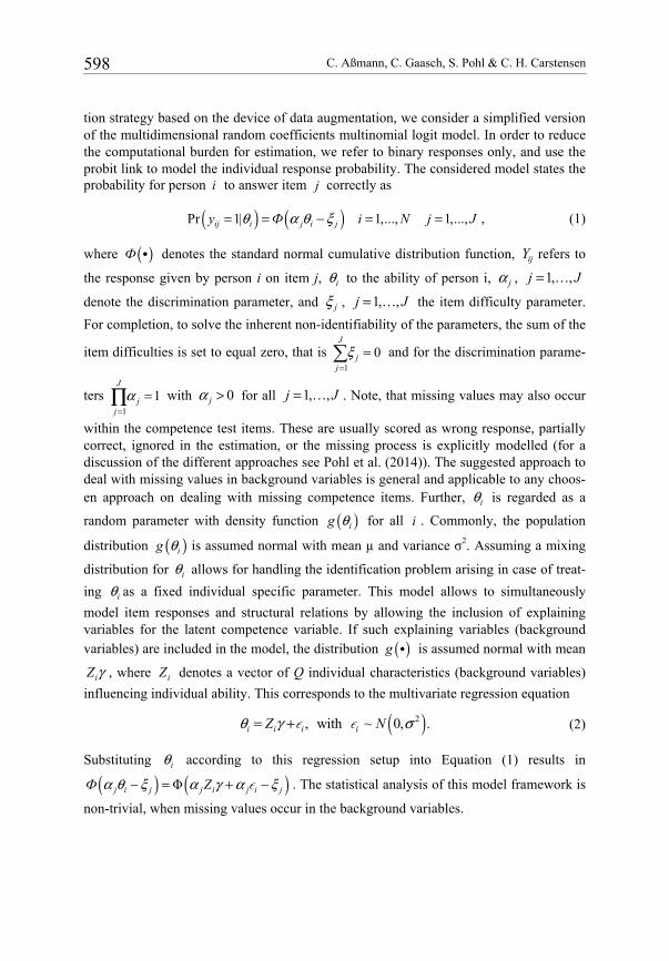
tion strategy based on the device of data augmentation, we consider a simplified version of the multidimensional random coefficients multinomial logit model. In order to reduce the computational burden for estimation, we refer to binary responses only, and use the probit link to model the individual response probability. The considered model states the probability for person i to answer item j correctly as

( ) ( )Pr 1| 1,..., 1,...,ij i j i jy Ф i N j Jθ α θ ξ= = − = = , (1)

where ( )Ф C denotes the standard normal cumulative distribution function, ijY refers to

the response given by person i on item j, iθ to the ability of person i, jα , 1, ,j J= …

denote the discrimination parameter, and jξ , 1, ,j J= … the item difficulty parameter.

For completion, to solve the inherent non-identifiability of the parameters, the sum of the

item difficulties is set to equal zero, that is 1

0J

jj

ξ=

= and for the discrimination parame-

ters 1

1J

jj

α=

=∏ with 0jα > for all 1, ,j J= … . Note, that missing values may also occur

within the competence test items. These are usually scored as wrong response, partially correct, ignored in the estimation, or the missing process is explicitly modelled (for a discussion of the different approaches see Pohl et al. (2014)). The suggested approach to deal with missing values in background variables is general and applicable to any choos-en approach on dealing with missing competence items. Further, iθ is regarded as a

random parameter with density function ( )ig θ for all i . Commonly, the population

distribution ( )ig θ is assumed normal with mean µ and variance σ2. Assuming a mixing

distribution for iθ allows for handling the identification problem arising in case of treat-

ing iθ as a fixed individual specific parameter. This model allows to simultaneously

model item responses and structural relations by allowing the inclusion of explaining variables for the latent competence variable. If such explaining variables (background variables) are included in the model, the distribution ( )g C is assumed normal with mean

iZ γ , where iZ denotes a vector of Q individual characteristics (background variables)

influencing individual ability. This corresponds to the multivariate regression equation

( )2 , with ~ 0, .i i i iZ Nθ γ σ= + (2)

Substituting iθ according to this regression setup into Equation (1) results in

( ) ( )Φj i j j i j i jФ Zα θ ξ α γ α ξ− = + − . The statistical analysis of this model framework is

non-trivial, when missing values occur in the background variables.


3 The proposed approach for dealing with missing values in person background variables within IRT models

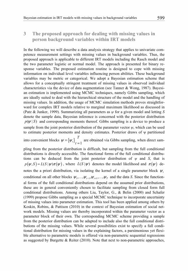
In the following we will describe a data analysis strategy that applies to univariate com-petence measurement settings with missing values in background variables. Thus, the proposed approach is applicable to different IRT models including the Rasch model and the two parameter logistic or normal model. The approach is presented for binary re-sponse variables. The proposed estimation routine is designed to cope with missing information on individual level variables influencing person abilities. These background variables may be metric or categorical. We adopt a Bayesian estimation scheme that allows for a conceptually stringent treatment of missing values in observed individual characteristics via the device of data augmentation (see Tanner & Wong, 1987). Bayesi-an estimation is implemented using MCMC techniques, namely Gibbs sampling, which are ideally suited to deal with the hierarchical structure of the model and the handling of missing values. In addition, the usage of MCMC simulation methods proves straightfor-ward for complex IRT models relative to marginal maximum likelihood as discussed in (Patz & Junker, 1999). Summarizing all parameters as ψ for a given model and letting S denote the sample data, Bayesian inference is concerned with the posterior distribution

( | )p Sψ and corresponding moments thereof. Gibbs sampling is a device to produce a

sample from the joint posterior distribution of the parameter vector ψ, which can be used to estimate posterior moments and density estimates. Posterior draws of ψ partitioned

into convenient blocks 1t

T

tψ ψ=

= are obtained via Gibbs sampling, when direct sam-

pling from the posterior distribution is difficult, but sampling from the full conditional distributions is directly accessible. The functional forms of the full conditional distribu-tions can be deduced from the joint posterior distribution of ψ and S, that is

( ) ( ), ( | )p S L Sψ ψ π ψ= , where ( | )L S ψ denotes the model likelihood and ( )π ψ de-

notes the a priori distribution, via isolating the kernel of a single parameter block tψ

conditional on all other blocks 1 1 1, , , , ,t t Tψ ψ ψ ψ− +… … and the data S. Since the function-

al forms of the full conditional distributions depend on the assumed prior distributions, these are in general conveniently chosen to facilitate sampling from closed form full conditional distributions. Among others Liu, Taylor, G., & Belin (2000) and Schafer (1999) propose Gibbs sampling as a special MCMC technique to incorporate uncertainty of missing values into parameter estimation. This tool has been applied among others by Koskin, Robins, & Pattison (2010) in the context of Bayesian estimation of social net-work models. Missing values are thereby incorporated within the parameter vector as a parameter block of their own. The corresponding MCMC scheme providing a sample from the posterior distribution can be adapted to include also the full conditional distri-butions of the missing values. While several possibilities exist to specify a full condi-tional distribution for missing values in the explaining factors, a parsimonious yet flexi-ble alternative to parametric models is offered via non-parametric sequential regressions as suggested by Burgette & Reiter (2010). Note that next to non-parametric approaches,


also semi-parametric approaches based on chained equations are available (see van Buuren & Groothuis-Oudshoorn, 1987).

3.1 Estimation algorithm

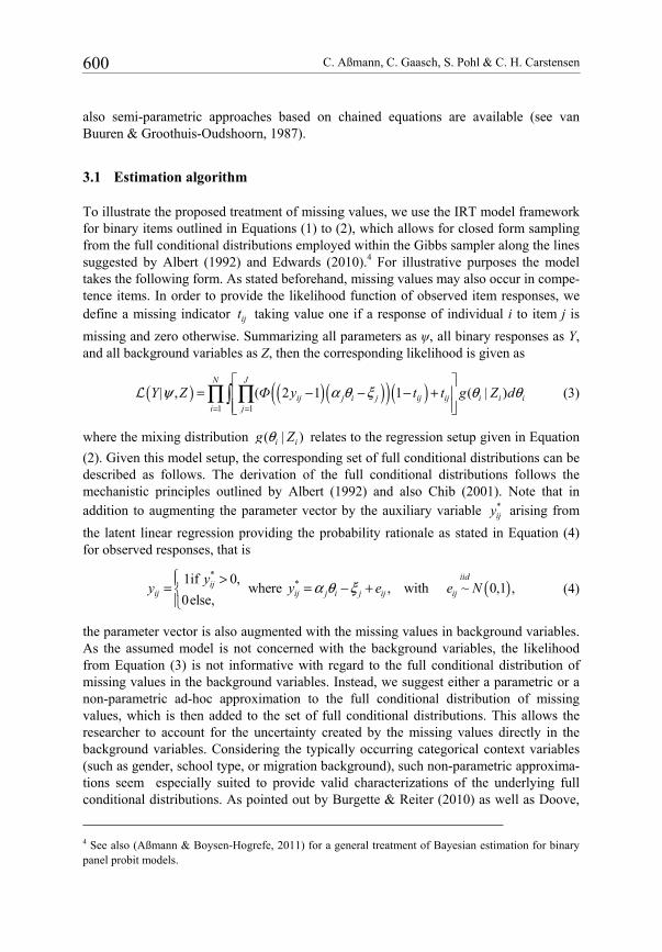
To illustrate the proposed treatment of missing values, we use the IRT model framework for binary items outlined in Equations (1) to (2), which allows for closed form sampling from the full conditional distributions employed within the Gibbs sampler along the lines suggested by Albert (1992) and Edwards (2010).4 For illustrative purposes the model takes the following form. As stated beforehand, missing values may also occur in compe-tence items. In order to provide the likelihood function of observed item responses, we define a missing indicator ijt taking value one if a response of individual i to item j is

missing and zero otherwise. Summarizing all parameters as ψ, all binary responses as Y, and all background variables as Z, then the corresponding likelihood is given as

( ) ( )( )( )( )1 1

| , ( 2 1 1 ( | )N J

ij j i j ij ij i i ii j

Y Z Ф y t t g Z dψ α θ ξ θ θ= =

= − − − +

∏ ∏ (3)

where the mixing distribution ( | )i ig Zθ relates to the regression setup given in Equation

(2). Given this model setup, the corresponding set of full conditional distributions can be described as follows. The derivation of the full conditional distributions follows the mechanistic principles outlined by Albert (1992) and also Chib (2001). Note that in addition to augmenting the parameter vector by the auxiliary variable *

ijy arising from

the latent linear regression providing the probability rationale as stated in Equation (4) for observed responses, that is

( )*

*1 if 0, where with 0,1 ,

0 else, , ~

ij

ij ij

i

j i j i

d

j

i

j i

yy y e e Nα θ ξ

>= = − +

(4)

the parameter vector is also augmented with the missing values in background variables. As the assumed model is not concerned with the background variables, the likelihood from Equation (3) is not informative with regard to the full conditional distribution of missing values in the background variables. Instead, we suggest either a parametric or a non-parametric ad-hoc approximation to the full conditional distribution of missing values, which is then added to the set of full conditional distributions. This allows the researcher to account for the uncertainty created by the missing values directly in the background variables. Considering the typically occurring categorical context variables (such as gender, school type, or migration background), such non-parametric approxima-tions seem especially suited to provide valid characterizations of the underlying full conditional distributions. As pointed out by Burgette & Reiter (2010) as well as Doove,

4 See also (Aßmann & Boysen-Hogrefe, 2011) for a general treatment of Bayesian estimation for binary panel probit models.


van Buuren, & Dusseldorp (2014), the flexibility of non-parametric approaches to cope also with non-linear dependency and non-standard interactions possibly the challenges inherent to statistical analysis with missing data.

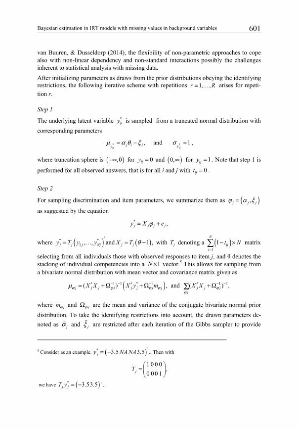
After initializing parameters as draws from the prior distributions obeying the identifying restrictions, the following iterative scheme with repetitions 1, ,r R= … arises for repeti-

tion r.

Step 1

The underlying latent variable *ijy is sampled from a truncated normal distribution with

corresponding parameters

* *, and 1ij ij

j i jy yμ α θ ξ σ= − = ,

where truncation sphere is ( ),0−∞ for 0ijy = and ( )0,∞ for 1ijy = . Note that step 1 is

performed for all observed answers, that is for all i and j with 0ijt = .

Step 2

For sampling discrimination and item parameters, we summarize them as ( ),j j jϕ α ξ=

as suggested by the equation

* ,j j j jy X eϕ= +

where ( ) ( )'* *1 , , and 1 ,j j j Nj j jy T y y X T θ= … = − with jT denoting a ( )

1

1N

iji

t N=

− × matrix

selecting from all individuals those with observed responses to item j, and θ denotes the stacking of individual competencies into a 1N × vector.5 This allows for sampling from a bivariate normal distribution with mean vector and covariance matrix given as

( )1 1 * 1 1 1( ) , and ( ) ,j j j j j j j j j j jj

X X X y m X Xϕ ϕ ϕ ϕ ϕϕ

μ − − − − −= + Ω + Ω ′ Ω′ +′ Σ

where jmϕ and jϕΩ are the mean and variance of the conjugate bivariate normal prior

distribution. To take the identifying restrictions into account, the drawn parameters de-

noted as jα and jξ are restricted after each iteration of the Gibbs sampler to provide

5 Consider as an example. ( )'* 3.5 3.5jy NA NA= − .. Then with

1 0 0 0

0 00 1jT

=

,

we have ( )* 3.5 3.5 'j jT y = − .


new draws used in the successive steps, that is 1/( )

jj J J

jj

αα

α=

∏

and

1

1 J

j j jjJ

ξ ξ ξ=

= − .

Sampling is done for all 1,j J= … .

Step 3

The individual abilities iθ are sampled from a full conditional normal distribution. With

iT denoting a ( )1

1J

ijj

t J=

− × matrix selecting all items with observed responses from

individual i, define ( )*i i iy T y ξ= − and i iX Tα= , where *, iyα and ξ denote the vectors

of all J discrimination parameters, latent variables or difficulties. This allows for stating the moments and variance of the full conditional multivariate normal distribution as

( ) 2 1 2 2 2 1( ) and ( )i i

i i ii i i iX X X y Z X Xθ θμ σ σ γ σ σ− − − − −′ ′ ′= + + = + .

Sampling is performed for all 1, ,i N= … . In accordance with the assumed model struc-ture, individual abilities iθ are sampled conditional on observed responses and back-ground variables.

Step 4

Draws from full conditional distribution for γ are obtained from a multivariate normal distribution with corresponding moments given as

1 11 1 1

2 2 2 and

Z Z Z Z Zγ γ γ γ γ γ

θμ νσ σ σ

− −− − − = + Ω + Ω Σ = + Ω

′ ′ ′

with Z denoting the matrix of background variables, γν and covariance matrix γΩ de-noting the moments of corresponding conjugate normal prior distribution.

Step 5

Choosing the independent conjugate prior for 2σ as inverse gamma with parameters 0a and 0b , then the full conditional of 2σ is also distributed inverse gamma with corre-sponding parameters

( )1

20 0

1

1, and .

2 2

N

i ii

Na a b Z bθ γ

−

=

= + = − +

Step 6

As the parameter vector is augmented with the missing values in background variables, corresponding draws are either obtained based on parametric approximations to the full conditional distributions or on non-parametric approximations to the full conditional


distributions. While a parametric approximation is efficient for dealing with metric background variables and known dependencies, the non-parametric approach allows for flexible handling of categorical background variables and is capable to account for non-linear dependencies among the variables. The following set of conditioning variables

denoted as matrix ( ), , ,q qW Z SCι θ−= is considered, where ι denotes a vector of N ones,

qZ− the matrix of background variables except variable qZ , and SC denotes a vector of

sample statistics, for example the sum score, of the competence items for each individu-al. Note that the draws for the missing values in the background variables are based upon the competence score θ and, thus, the latent ability is incorporated in the imputation. Note that if no missing values are present within the responses to the competence items, using the sum score as a sample statistic of observed item responses may not enrich the model with further information, as the sum score may be subsumed within the vector of latent abilities θ.

a) When using a parametric approximation to the full conditional distribution of the missing values, draws for the missing values in the N Q× matrix of background

variables Z can be obtained via specifying a univariate normal full conditional dis-tribution for each of the Q variables contained in Z. Within the intercourse of the Gibbs sampler, imputed and hence complete variables are at hand for each iteration r, resulting in the following Q regression equations given as , 1, ,q q q qZ W q Qϕ= + = … .

Imputations are then generated as follows. Each missing value in qZ is replaced via

a draw from a univariate normal distribution with expectation ˆ'misW ϕ and variance

2σ . To account for the uncertainty of the least squares estimators ϕ and 2σ ,

draws from the corresponding asymptotic distributions are used for generating draws for the missing values in qZ . Further, it should be explicitly noted that the es-

timation scheme introduces the updated draws of the individual latent abilities θ into the imputation model for each iteration and that a parametric scheme becomes com-putationally burdensome for missing values in discrete variables with many catego-ries.

b) In order to establish flexible approximations to the full conditional distributions of missing values in background variables Z, Burgette & Reiter (2010) suggest to use nonparametric approximations obtained via Classification and Regression Trees CART (see Breiman, Friedman, Olshen, & Stone, 1984). The flexibility of the CART algorithm to incorporate nonlinear dependencies among the variables with missing data has been highlighted by Doove et al. (2014). CART constitutes a non-parametric recursive partition algorithm. The objective of CART is to split up the observations into different groups, fulfilling the condition that respondents and thus observations assigned to one group show highest intra-group homogeneity with re-spect to the relevant variable, whereas the inter-group homogeneity is intended to be as small as possible. There exist manifold possibilities to define a partition. CART


defines binary partitions via a set of conditioning variables. In the present applica-tion the set of conditioning variables containing all available information is given via qW . To ensure computational feasibility, the CART algorithm does consider

univariate splits only, that is only binary partitions defined upon a single variable are considered. The sequential partitioning algorithm proceeds via consideration of all binary parti-tions. Of all possible binary partitions defined by univariate splits, the split with the maximum reduction in heterogeneity is selected as the optimal partition. As indica-tors for heterogeneity the variance in case of metric and the entropy in case of cate-gorical variables are chosen. The resulting binary partition of the data along the set of conditioning variables provides sets of admissible values defining the nonpara-metric characterization of the full conditional distribution and serving as donors for filling in the missing values. All respondents can be assigned to one of these identi-fied donor groups. Each missing value is imputed via a draw from the empirical dis-tribution within this donor group using a Bayesian bootstrap. Thus, the uncertainty of the unobserved missing values is directly taken into account in parameter estima-tion. With regard to the settings of the CART algorithm, concerning stopping crite-ria and minimum requirements for the size of donor groups, we follow the sugges-tions of Burgette & Reiter (2010). Hence, no further split is considered when the re-sulting reference groups contain less than 50 or the gain in homogeneity is less than 0.01.

Given a sample of all model parameters obtained via iterative sequential cycling through the set of full conditional distributions, the plausible values for each individual can be directly taken from the provided Gibbs output. After discarding an appropriate burn-in

phase each sweep 1, 1, ,

Ri r

i nθ=

= … from the posterior distribution could be taken as a

vector of plausible values. The proposed approach simultaneously deals with the estima-tion of plausible values and the imputation of missing values in background variables, thus, accounting for both sources of uncertainty.

3.2 Simulation study

To assess the statistical validity of the proposed approach, we set up a simulation design investigating the statistical accuracy of parameter estimation. Within this design we compare the Bayesian data augmentation approach to handle missing values with the Bayesian full sample estimates before deletion and those from a Bayesian complete case analysis in which cases with missing values in background variables are deleted listwise. Further, we assess the parametric and the non-parametric approximation towards the full conditional distribution of missing values. The before deletion situation is thereby cho-sen as a benchmark providing estimators with highest possible statistical accuracy for a given data set, whilst the complete case situation illustrates reduced efficiency in pa-rameter estimation when ignoring missing values. The simulation study builds upon


repeated estimation of simulated data sets. Different data and missing values generating mechanisms are considered. The data sets with missing values in the background varia-bles are generated based on the complete data sets. Then for each of the complete data sets the corresponding Bayesian estimates before deletion are calculated, while for each of the data sets with missing values the Bayesian estimates based on data augmentation for handling of missing values are calculated. The estimates using data augmentation are compared to the estimates before deletion and the complete cases, when all individuals with missing values in the background variables are removed from the data set.

The detailed conditions of the data generating and missing values generating processes are as follows. For each of the 200C = replications, the binary response pattern to com-petence items is simulated using the model stated in Equations (1) and (2) with a sample setup of 1000N = individuals facing 10J = items. The item difficulty parameters are

fixed across the replications. To fulfil the implemented identifying restriction 1

0J

Jj

ξ=

=

they are derived as 1

1 J

j j jjJ

ξ ξ ξ=

= − , where ( )0,0.5 , 1 ,j N Jξ ∼ … are draws from a

normal distribution. Correspondingly, to ensure the positivity and scaling constraint on the discrimination parameters, these are generated as transformed draws from a lognor-

mal distribution, that is

( )1/

1

jj JJ

jj

u

uα

=

=∏

with ( )3,0.25 for 1, , ju LN j J∼ = … . For

each data set, four background variables , 1, ,4qZ q = … , explaining differences in indi-

vidual abilities iθ are generated from a multivariate normal distribution, where each

variable has mean of zero, unit variance, and pairwise correlation equal to 0.5. The fol-lowing transformations were applied to the variables. 2Z is squared, 3Z is transformed

into a dichotomous variable with split at a value of 0, and 4Z is categorized into a 4-way

categorical variable by its quartiles. The regression coefficients including an intercept are set to ( )1.0,0.5, 0.5,0.5, 0.25, 0.5, 1γ = − − − − for the corresponding set of background

variables given as

( ) ( )21 2 3 4 25 25 4 50 50 4 750,1 0,1 0,1 0,11, , , 0 , ( ), ( ), ( ) Z Z Z I Z I Z q I q Z q I q Z q= < < < < < < .

The individual abilities are then generated as draws from a normal distribution with

mean as implied by Zγ and a conditional variance parameter of 2 1.44σ = . Given val-

ues for the individual abilities, the latent variables *ij j i j ijy eα θ ξ= − + are calculated with

ije given as independent draws from a standard normal distribution and then dichoto-

mized according to *

0,1 ( 0)ij ijy I y= < .

Missing values are generated as follows. We distinguish two missing data generating mechanisms, which differ in their severity. With regard to data generating mechanism I


on average 5% missing values in 1Z and 10% missing values in 2Z were generated

completely at random. For data generating mechanism II the rates of missingness in-crease to 10% and 20% and depend on variable 3Z according to

( ) ( )1 3Pr 0.5 0.5i iZ NA Ф Z= = − − , and ( ) ( ) ( )2 4 3Pr Pr 1.5 0.5i i iZ NA Z NA Ф Z= = = = − + .

Thus, data generating mechanism II poses more challenges on the estimation routine than data generating mechanism I. Further note, that the data generating mechanism I is in line with the parametric approximation of the full conditional distribution for the augmented missing values, while missing data generating mechanism II with missing values in the categorical variable is not accessible to the parametric approximation of the full conditional distribution of the missing values.

Each of the repeated estimations for the total of 200C = data sets is based on MCMC sequences with each having a length of 2000 iterations. Inspection of time series and autocorrelation plots for all parameters indicates convergence. After discarding the first quarter of the samples as burn-in, inference is based on the remaining 1500 simulated draws from the joint posterior distribution. For evaluation of the results, the parameter estimates using the data augmentation approach are compared to those before deletion and complete cases via inspection of average estimates, the root mean squared errors, and the proportion of 95% highest posterior density regions that contain the true parame-ter values, that is coverages.

For the missing data generating mechanism I Table 1 shows the true parameter values, the means of the posterior expected values, their standard deviations, root mean squared errors (RMSE), and coverages over 200C = replications for all considered estimation approaches, that is the before deletion ( BD ), the complete case analysis ( CC ), the parametric ( PI ), and the non-parametric ( NPI ) imputation method. For the BD esti-mators we find overall unbiased estimation results for all parameters with all correspond-ing coverages reaching their nominal level as expected. Also, average standard devia-tions and RMSE coincide, thus highlighting the statistical accuracy of estimation in the case without missing values. Similar results are revealed for the PI estimators. Note that the implemented parametric imputation model using full conditional normal distri-butions reflects completely the chosen simulation setup making use of the normal distri-bution. Hence, in this setup the PI procedure is the most efficient way to handle miss-ing values in the estimation. In this sense, the statistical accuracy of the PI approach serves as a benchmark for the NPI approach. Within the considered simulation study, the NPI approach reveals unbiased estimation of all parameters. Further, inspection of the statistical accuracy in terms of the RMSE and coverages suggest no severe loss of statistical accuracy compared to the BD and the parametric approach. For example, the mean standard deviation of the regression parameter 4γ almost equals its RMSE, which

is in line with the findings for the BD and PI estimators. Also with respect to the cov-erage rates, the findings support that there is no notable difference to the BD estimators reported in the first block columns of Table 1. The observed number of intervals cover-ing the particular parameter corresponds to their expected theoretical values, for example

Bayesian estimation in IRT models with missing values in background variables 607T

able

1:

M

issi

ng d

ata

mec

hani

sm I

- M

CA

R

Not

es:

Ave

rage

pos

teri

or m

eans

and

sta

ndar

d de

viat

ion,

roo

t m

ean

squa

red

erro

r an

d co

vera

ge o

f C

=200

rep

lica

tions

for

a d

ata

set

befo

re d

elet

ion

(BD

), c

ompl

ete

case

an

alys

is (

CC

), th

e pa

ram

etri

c im

puta

tion

met

hod

(PI)

, and

the

non-

para

met

ric

impu

tati

on m

etho

d (N

PI).

C. Aßmann, C. Gaasch, S. Pohl & C. H. Carstensen 608T

able

2:

M

issi

ng d

ata

mec

hani

sm I

I -

MA

R

Not

es: A

vera

ge p

oste

rior

mea

ns a

nd s

tand

ard

devi

atio

ns, r

oot m

ean

squa

red

erro

r an

d co

vera

ge o

f C

=20

0 re

plic

atio

ns f

or a

dat

a se

t bef

ore

dele

tion

(B

D),

com

plet

e ca

se a

naly

sis

(CC

), a

nd th

e no

n-pa

ram

etri

c im

puta

tion

met

hod

(NP

I).


a 95% binomial proportion interval allows the coverages to lie between [0.907; 0.993] at 200C = replications for all considered parameters. For all considered estimation ap-

proaches, the 95% highest density intervals concur with this range.

The results for the simulation study considering the missing data to occur at random are presented in Table 2. Similarly to the results from the missing completely at random simulation design, the NPI method performs very well to estimate item parameters and the structural relations on individual abilities. Overall, inspection of the simulation re-sults suggests again high statistical accuracy of the suggested data augmentation ap-proach. For instance, the mean standard deviations of the regression parameters differ from their corresponding RMSEs only modestly. This is supported by the reported cov-erage rate, which meets the expected level of 95% for all estimated parameters.

Given the evidence from the simulation study, we conclude that the nonparametric ap-proach provides a valid and highly flexible approximation to the full conditional distribu-tion of missing values. Given the almost negligible loss in statistical accuracy compared to the benchmark BD and PI estimators, we suggest that the use of data augmentation using non-parametric devices is a suitable solution for dealing with partially observed background variables in the context of IRT models, regardless of the scaling type of background variables.

3.3 Empirical application

To illustrate the applicability of the suggested estimation approach, we provide an exem-plary empirical analysis, where we use data from the NEPS cohort sample of students in fifth grade (Blossfeld, Roßnach, & Maurice, 2011). For a description of the assessment of mathematical competence in NEPS, see Weinert, et al. (2011) and Neumann, Durchhardt, Ehmke, Grüßing, & Knopp (2013). Duchhardt & Gerdes (2012) provides an overview of the respective competence data and Skopek, Pink, & Bela (2013) the data manual of the corresponding scientific use file. The data used in this analysis contains student information on the first panel wave in the year 2010. We restrict our sample to the cases where parental information is available and to students with a valid response to at least one of the 23J = binary mathematics test items. The sample considered in our analyses consists of N 3615= students and their parents. Consistent with the scaling in the NEPS (Pohl & Carstensen, 2012; Pohl, Gräf, & Rose, 2014), missing values on test items set are ignored. To check the robustness of this approach, we further provide the estimation results based on cases with complete background variables only (N = 2955).

We consider several background variables on student level to gauge their impact on mathematical competence. These are gender, a dummy variable indicating if the student is a German native speaker or not, students mathematical self-concept, and satisfaction with school. Additionally, we include years of education of the parent who is responsible for the everyday issues of the child and the amount of books at home (ordinal variables) as indicators of the socio-economic and cultural context. Descriptive statistics for the data considered in the application are displayed in Table 3. With at most 6% univariate


Table 3: Descriptive statistics for backround variables.

Variable min max mean sd missing

categorical female 0 1 0.48 - 0%

non German native speaker 0 1 0.11 - 2%

number of books 0 5 - - 5%

continuous self-concept 1 4 2.95 0.84 6%

school satisfaction 0 10 7.74 2.94 3%

parent years of education 8 18 13.90 2.94 4%

Notes: N=3615

missing values, namely for mathematical self-concept, the total amount of missing data is considered to be relatively small.

We apply the proposed data augmented Gibbs sampling approach based on the nonpara-metric approximation of the full conditional distribution of missing values for estimating the regression coefficients relating background variables and the latent mathematics competence. The trace plots show no indication of convergence problems (Figure 1, Figure 2, and Figure 3). The observed autocorrelations are low, and also the cumulative means indicate no converge problems at all. Taken a burn-in period of 2000 draws, all parameter estimates are based on 8000 simulated draws. Table 4 depicts the estimated posterior means and standard deviations, as well as the 95% highest density intervals. While the results indicate a lower level of competence for females and non German native speakers, mathematical self-concept, and school satisfaction have a positive effect on students mathematical abilities. Both, a higher level of parental education and a high-er number of books available in the household, are positively associated with students’ mathematical ability (with all other predictors assumed constant). Note that the regres-sion coefficients reflect the relationship of questionnaire variables with latent mathemat-ics scores that are purified from measurement error. The estimated standard errors of the regression coefficients incorporate not only the uncertainty due to person sampling, but also uncertainty due to missing values in the predictors. Comparison with the results obtained for cases with complete background variables reveals no substantial differences. However, all parameter estimates based on complete cases only have higher standard deviations. This illustrates the increased efficiency of the suggested data augmentation approach to handle missing values in background variables.


Figure 1: Trace plots for the regression constant ( 1γ ), the regression coefficients for sex ( 2γ ), German

native speaker ( 3γ ), mathematical self-concept ( 4γ ), school satisfaction ( 5γ ), years of education parent ( 6γ ), number of books at home ( 7 8 9 10 11, , , ,γ γ γ γ γ ), as well as the residual

variance ( 2σ ).


Figure 2: Trace plots for the discrimination parameters ( jα , 1, ,j J= … ).


Figure 3:

Trace plots for the difficulty parameters ( , = 1, … , )


Table 4: Mathematical competencies: Parameter estimates of random coefficient IRT model

Non-parametric imputation Complete cases N=3615 N=2955 Parameter mean sd 95% HDI mean sd 95% HDI

γ1 (constant) −1.202 0.071 [-1.344;-1.062] −1.183 0.082 [-1.344;-1.027] γ2 (female) −0.098 0.017 [-0.131;-0.064] −0.112 0.019 [-0.150;-0.075] γ3 (nongerman) −0.156 0.026 [-0.209;-0.105] −0.189 0.033 [-0.256;-0.123] γ4 (selfconcept) 0.147 0.010 [0.127;0.168] 0.154 0.012 [0.131;0.177] γ5 (schoolsat) 0.016 0.003 [0.009;0.022] 0.017 0.004 [0.009;0.024] γ6 (peduc) 0.054 0.004 [0.047;0.061] 0.052 0.004 [0.044;0.060] γ7 (nobooks1) 0.066 0.051 [-0.034;0.165] 0.079 0.060 [-0.040;0.195] γ8 (nobooks2) 0.213 0.048 [0.122;0.308] 0.226 0.056 [0.113;0.336] γ9 (nobooks3) 0.293 0.048 [0.198;0.390] 0.308 0.057 [0.196;0.422] γ10 (nobooks4) 0.399 0.050 [0.302;0.498] 0.415 0.058 [0.300;0.527] γ11 (nobooks5) 0.389 0.051 [0.289;0.489] 0.421 0.059 [0.304;0.538] σ^2 0.162 0.006 [0.151;0.175] 0.166 0.007 [0.153;0.180] α1 1.142 0.059 [1.025;1.258] 1.116 0.064 [0.989;1.243] α2 1.199 0.061 [1.082;1.320] 1.240 0.068 [1.109;1.376] α3 1.057 0.056 [0.951;1.169] 1.045 0.063 [0.922;1.170] α4 0.789 0.050 [0.691;0.888] 0.822 0.057 [0.712;0.933] α5 1.229 0.058 [1.116;1.341] 1.192 0.065 [1.068;1.323] α6 0.752 0.047 [0.661;0.844] 0.768 0.051 [0.669;0.870] α7 1.374 0.063 [1.253;1.499] 1.397 0.069 [1.263;1.536] α8 1.050 0.064 [0.928;1.178] 1.075 0.072 [0.936;1.217] α9 1.271 0.079 [1.121;1.427] 1.223 0.091 [1.046;1.404] α10 1.399 0.064 [1.276;1.527] 1.322 0.069 [1.190;1.458] α11 1.201 0.055 [1.095;1.310] 1.179 0.062 [1.060;1.302] α12 0.662 0.050 [0.563;0.760] 0.687 0.055 [0.581;0.799] α13 0.674 0.050 [0.575;0.770] 0.713 0.054 [0.609;0.817] α14 0.934 0.057 [0.822;1.046] 0.895 0.062 [0.773;1.018] α15 1.120 0.059 [1.004;1.237] 1.085 0.065 [0.959;1.214] α16 0.997 0.059 [0.883;1.114] 0.982 0.068 [0.847;1.116] α17 1.019 0.054 [0.914;1.125] 1.064 0.061 [0.944;1.184] α18 0.880 0.048 [0.787;0.976] 0.889 0.054 [0.782;0.993] α19 1.050 0.054 [0.946;1.156] 1.015 0.059 [0.901;1.130] α20 0.748 0.048 ][0.654;0.843] 0.763 0.052 [0.659;0.863] α21 0.795 0.062 [0.672;0.914] 0.789 0.071 [0.651;0.928] α22 1.122 0.055 [1.015;1.231] 1.081 0.060 [0.965;1.198] α23 1.092 0.053 [0.990;1.198] 1.155 0.061 [1.035;1.276] ξ1 0.069 0.027 [0.016;0.121] 0.052 0.030 [-0.005;0.113] ξ2 −0.270 0.025 [-0.319;-0.220] −0.246 0.030 [-0.306;-0.187] ξ3 −0.177 0.026 [-0.228;-0.127] −0.189 0.030 [-0.246;-0.131]


Non-parametric imputation Complete cases N=3615 N=2955 Parameter mean sd 95% HDI mean sd 95% HDI

ξ4 0.662 0.028 [0.607;0.717] 0.687 0.033 [0.622;0.750] ξ5 0.269 0.027 [0.217;0.321] 0.253 0.031 [0.193;0.314] ξ6 0.374 0.025 [0.325;0.424] 0.384 0.029 [0.327;0.441] ξ7 0.687 0.031 [0.627;0.748] 0.706 0.036 [0.638;0.778] ξ8 −0.724 0.027 [-0.777;-0.672] −0.725 0.030 [-0.784;-0.665] ξ9 −1.062 0.030 [-1.123;-1.002] −1.082 0.034 [-1.147;-1.016] ξ10 0.055 0.027 [0.003;0.107] 0.034 0.030 [-0.026;0.093] ξ11 −0.058 0.025 [-0.107;-0.010] −0.056 0.029 [-0.113;0.000] ξ12 0.858 0.029 [0.801;0.915] 0.872 0.034 [0.805;0.938] ξ13 0.118 0.026 [0.068;0.167] 0.145 0.029 [0.087;0.202] ξ14 −0.394 0.026 [-0.446;-0.343] −0.425 0.030 [-0.484;-0.367] ξ15 −0.428 0.026 [-0.478;-0.378] −0.438 0.029 [-0.494;-0.382] ξ16 −0.728 0.026 [-0.780;-0.679] −0.769 0.030 [-0.827;-0.710] ξ17 0.024 0.025 [-0.025;0.074] 0.036 0.029 [-0.021;0.094] ξ18 0.134 0.024 [0.087;0.182] 0.153 0.028 [0.098;0.209] ξ19 0.383 0.027 [0.331;0.435] 0.375 0.031 [0.313;0.436] ξ20 0.580 0.026 [0.529;0.631] 0.602 0.030 [0.542;0.661] ξ21 −0.945 0.028 [-0.999;-0.891] −0.962 0.032 [-1.027;-0.900] ξ22 0.138 0.026 [0.087;0.188] 0.125 0.029 [0.068;0.182] ξ23 0.439 0.027 [0.387;0.491] 0.468 0.032 [0.406;0.530]

4 Conclusion

In large scale assessments researchers are usually interested in explaining competence scores by individual characteristics and context variables. Measurement error in compe-tence scores as well as missing values in background variables capturing individual characteristics and context variables need to be accounted for. We propose a Bayesian data augmented MCMC approach that simultaneously estimates plausible values and accounts for missing values in background variables. With this approach latent relation-ships between competence scores and background variables may be estimated, which efficiently incorporate the uncertainty stemming from only partially observed back-ground variables into parameter estimation. Especially the iterative use of updated pa-rameter values from posterior sampling within the full conditional distribution of missing values is an appealing feature of our approach. Treatment of missing values in back-ground variables using the device of data augmentation further has the advantage that, in contrast to approaches using dummy indicators to model missingness of values, the interpretability of parameters governing the relationship between background variables and competencies remains the same as in situations with completely observed back-ground variables. In a simulation study the proposed approach shows high statistical


accuracy as well as the ability to adequately recover the model parameters, even when higher rates of missing values occur in the data. The applicability to educational large scale research data has been illustrated via an empirical example.

So far, in large scale assessments the issue of missing values in background variables of IRT models has been typically approached by a two-step procedure, first accounting for missing values in background variables using indicator variables and then estimating plausible values. With this procedure, the latent competence is not efficiently included in the imputation of the background variables and the uncertainty stemming from the impu-tation is not directly accounted for. The proposed approach in this paper allows for sim-ultaneously accounting for measurement error and missing values in background varia-bles and, thus, efficiently incorporates both sources of uncertainty in the parameter and variance estimation. This approach is not only applicable to competence measurement in large scale studies, but to any study in which relationships are estimated for latent con-structs with explaining variables that include missing values. The evidence from the simulation study documents that a moderate sample size of 1000 and 10 measurements per individual facilitate accurate parameter estimation, however, given the high accuracy, even smaller sample sizes may suffice.

Future research could focus on extending the suggested estimation approach towards other model frameworks and capturing the different demands of large scale assessment studies. Extending the proposed approach to incorporate other IRT models would strengthen its applicability in empirical studies. As many large scale studies apply a two-stage sampling scheme, drawing first from a set of schools and then from a set of stu-dents within these schools, incorporation of hierarchical structures within our estimation approach would also extend the applicability of the suggested approach. Furthermore, often more than one competence is of interest or change in competence scores is consid-ered. In future research the proposed approach could be extended to multidimensional models including both within and between multidimensionality.

Acknowledgements

This paper uses data from the National Educational Panel Study (NEPS): Starting Cohort 3 '- 5th grader (Schule, Ausbildung und Beruf), doi:10.5157/NEPS:SC3:1.0.0. From 2008 to 2013, NEPS data were collected as part of the Framework Programme for the Promotion of Empirical Educational Research funded by the German Federal Ministry of Education and Research (BMBF). As of 2014, the NEPS survey is carried out by the Leibniz Institute for Educational Trajectories (LIfBi) at the University of Bamberg in cooperation with a nationwide network. Further, we thank the anonymous referees for the very constructive comments, which helped to improve this paper. The authors also gratefully acknowledge financial support by the Deutsche Forschungsgemeinschaft (DFG) for their research project (“Analyzing relations between latent competencies and context information in the National Educational Panel Study”) within the DFG priority programme 1646 (“Education as a Lifelong process”) under grants AS 368/3-1, PO 1655/2-1, and CA 289/8-1.


References

Albert, J. (1992). Bayesian estimation of normal ogive item response curves using gibbs sampling. Journal of Educational Statistics, 17, 251-269.

Allen, N., Carlson, J., Johnson, E., & Mislevy, R. (2001). Scaling procedures. U.S. Depart-ment of Education: The NAEP Technical Report.

Aßmann, C., & Boysen-Hofgrefe, J. (2011). A bayesian approach to model-based clustering for binary panel probit models. Computational Statistics & Data Analysis, 55, 261-279.

Aßmann, C., Gaasch, C., Pohl, S., & Carstensen, C. (2016). Estimation of plausible values considering partially missing backround information: A data augmented MCMC ap-proach. In H.-P. Blossfeld, J. von Maurice, J. Skopek, & M. Bayer (Eds.), Methological Issues of Longitudinal Surveys (pp. 505-522).Wiesbaden: Springer.

Béguin, A. A., & Glas, C. A. W. (2001). MCMC Estimation and some Model-Fit Analysis of Multidimensional IRT Models. Psychometrika, 66, 541-562.

Birnbaum, A. (1968). Some latent trait models and their use in inferring an examinee's ability. In F. M. Lord & M. R. Novick, Statistical theories of mental test scores (S. 397-479). Reading, MA: Addison-Wesley.

Blossfeld, H.-P., Roßnach, H.-G., & Maurice, J. (2011). Education as a Lifelong Process. The German National Educational Panel Study (NEPS) [Special Issue]. Zeitschrift für Erzie-hungswissenschaften, 14, 283-299. Wiesbaden: VS Verlag für Sozialwissenschaften Springer.

Breiman, L., Friedman, J. H., Olshen, R. A., & Stone, C. J. (1984). Classification and Regres-sion trees. Chapman & Hall.

Burgette, L., & Reiter, J. (2010). Multiple imputation for missing data via sequential regres-sion trees. American Journal of Epidemiology, 172, 1070-1076.

Chib, S. (2001). Markov Chain Monte Carlo Methods: Computation and inference. Handbook of Econometrics, 5, 3569-3649.

Doove, L., van Buuren, S., & Dusseldorp, E. (2014). Recursive partitioning for missing data imputation in the presence of interaction effects. Computational Statistics & Data Analy-sis, 72, 92-104.

Duchhardt, C., & Gerdes, A. (2012). Neps technical report for mathematics: Scaling results of starting cohort 3 in fifth grade. University of Bamberg: Leibniz Institute for Educational Trajectories.

Edwards, M. (2010). A Markov Chain Monte Carlo Approach to Confirmatory Item Factor Analysis. Psychometrika, 75, 474-497.

Koskin, J., Robins, G., & Pattison, P. (2010). Analysing exponential random graph (p-star) models with missing data using bayesian data augmentation. Statistical Methodology, 7, 366-384.

Liu, M., Taylor, J., G., M., & Belin, T. (2000). Multiple Imputation and Posterior Simulation for Multivariate Missing Data in Longitudinal Studies. Biometrics, 4, 1157-1163; 4(56).

Masters, G. (1982). A Rasch model for partial credit scoring. Psychometrika, 47, 149-174.


Mislevy, R. (1987). Exploiting auxiliary information about examinees in the estimation of item parameters. Applied Psychological Measurement, 11, 81-91.

Mullis, I., Martin, M., Foy, P., & Arora, A. (2012). TIMSS 2011 international results in math-ematics. Bosten College: MA: TIMSS & PIRLS International Study Center.

National Center for Education Statistics. (2013). The nation's report card: A first look: 2013 mathematics and reading (NCES 2014-451). Washington D.C.: Institution of Education Sciences, U.S. Department of Education.

Neumann, I., Durchhardt, C., Ehmke, T., Grüßing, M. H., & Knopp, E. (2013). Modeling and assessing of mathematical competence over the lifespan. Journal for Educational Re-search Online, 5, 80-109.

OECD. (2012). PISA 2009 Technical Report. OECD Publishing.

Patz, R., & Junker, B. (1999). A straightforward approach to Markov Chain Monte Carlo methods for item response models. Journal of Educational and Behavioral Statistics, 24, 146-178.

Pohl, S., & Carstensen, C. (2012). Scaling the data of the competence tests. NEPS Technical Report 14. Bamberg: Otto-Friedrich-University, Nationales Bildungspanel.

Pohl, S., Gräf, L., & Rose, N. (2014). Dealing with Omitted and Not-Reached Items in Com-petence Tests - Evaluating Approaches Accounting for Missing Responses in Item Re-sponse Theory Models. Educational and Psychological Measurement, 74, 423-452.

Rasch, G. (1960). Probabilistic Models for some Intelligence and Attainment Tests. Danish Institute for Educational Research.

Rubin, D. (1987). Multiple imputation for Nonresponse in Surveys. J. Wiley & Sons.

Schafer, J. (1999). Multiple Imputation: a primer. Statistical Methods in Medical Research, 8, 3-15.

Skopek, J., Pink, S., & Bela, D. (2013). Starting cohort 3: Grade 5 (sc3). suf version 1.0.0. data manual (neps research data paper). University of Bamberg, Leibniz Institute for Ed-ucational Trajectories, National Educational Panel Study.

Tanner, M., & Wong, W. (1987). The calculation of posterior distributions by data augmenta-tion. Journal of American Statistical Association, 92, 528-540.

van Buuren, S., & Groothuis-Oudshoorn, K. (1987). mice: Multivariate imputation by chain equations. Journal of Statistical Software, 45, 1-67.

Weinert, S., Artel, C., Prenzel, M., Senkbeil, M., Ehmke, T., & Carstensen, C. (2011). Devel-opment of competencies across the life span. Education as a Lifelong Process. The Ger-man National Educational Panel Study (NEPS), S. 67-86.

Documents

Bayesian estimation in IRT models with missing values in ... · Bayesian estimation in IRT models with missing values in background variables 597 approach is a two-step approach that