Ann. Inst. Statist. Math. Vol. 48, No. 1, 17-28 (1996)

BAYESIAN CALIBRATION IN THE ESTIMATION OF THE AGE OF RHINOCEROS

J. L. DU PLESSIS AND A. J. VAN DER MERWE

Department of Mathematical Statistics, Faculty o] Science, University of the O.F.S., P.O. Box 339, Bloemfontein, 9300, Republic of South Africa

(Received June 28, 1993; revised April 11, 1995)

Abstract . In this paper the Bayesian approach for nonlinear multivariate calibration will be illustrated. This goal will be achieved by applying the Gibbs sampler to the rhinoceros data given by Clarke (1992, Biometrics, 48(4), 1081- 1094). It will be shown that the point estimates obtained from the profile likelihoods and those calculated from the marginal posterior densities using improper priors will in most cases be similar.

Key words and phrases: Anterior horn length, multivariate Bayesian calibra- tion, nonlinear response model, credibility intervals, Gibbs sampler, posterior horn length, posterior distribution, rhinoceros data, Student-t family.

1. Introduction

The traditional calibration problem is concerned with estimating the unknown value of an explanatory variable x corresponding to an observed value of a response variable Y that is assumed to be functionally related to x. Since Krutchkoff's paper appeared in Technometrics (1967), a great deal has been written on the calibration problem, see for example, Hunter and Lamboy (1981), Scheff@ (1973) and Williams (1969). Brown (1982) gives a broad review of the linear multivariate calibration problem and outlines both Bayesian and non-Bayesian solutions. Oman and Wax (1984) consider an application of linear multivariate calibration in estimating fetal age, given two measurements, femur length and biparietal diameter on human babies. They comment on the nonlinear response model as being very difficult to analyse.

This paper is concerned with obtaining an estimate for an unknown value x corresponding to an observed Y, where Y and x are related through a nonlinear function. A Bayesian approach will be used to make inferences about the unknown x. The example that will be used is one from Clarke (1992). In this problem a sample of rhinoceros of known ages xi, i = 1 , . . . ,n have measurements made on the anterior (Yai) and posterior horn (Yp~). This data are to be used in future to predict a new fixed but unknown age x0 (denoted by ~) corresponding to the observed Y0 = [ya0 ypo]'.

17

18 J. L. DU PLESSIS AND A. J. VAN DER MERWE

The model proposed by Clarke (1992) is the classic multi-response model, (Bates and Watts (1988), Chapter 4) where the response functions are nonlinear in the unknown parameters. Clarke augmented the original data set with the additional measurements Ya0 and yp0 and a guessed age for ~0 of an extra animal whose age is needed. By varying values of (0 he generated varying values of the maximum likelihood, conditional on ~0, and these define the profile likelihood. This profile likelihood can be used and interpreted in a number of ways, all basically intended to illustrate the reliability of the age estimate.

As mentioned by Clarke "The step of associating the profile likelihood with classical confidence limits for the true value ~0 is difficult and only approximate solutions are available. To that extent this paper should not be regarded as propos- ing a definitive answer". Smith and Corbett (1987) pointed out that the profile likelihood often fails to tend to zero as {o ~ +oc so it cannot strictly be renormal- ized and treated as a posterior density. It therefore seems obvious that emphasis should be placed on Bayesian estimation of the model parameters.

Technical difficulties arising in the calculation of the marginal posterior densi- ties needed for Bayesian inference have long served as an impediment to the wider application of the Bayesian framework to real data. The reason for this is that the integration operation plays a fundamental role in Bayesian statistics. In the last few years there have been a number of advances in numerical integration and an- alytic approximation techniques for such calculations but implementation of these approaches typically requires sophisticated numerical or analytic approximation expertise and possibly specialist software.

Recently due to work of Gelfand and Smith (1991), Gelfand et al. (1990), Carlin et al. (1992) and Gelfand et al. (1992), the Gibbs sampler has been shown as a useful tool for applied Bayesian inference in a broad variety of statistical problems. The Gibbs sampler is implicit in the work of Hastings (1970) and made popular in the image processing context by Geman and Geman (1984). The Gibbs sampler is an adaptive Monte Carlo integration technique. The typical objective of the sampler is to collect a sufficiently large enough number of parameter real- izations from conditional posterior densities in order to obtain accurate estimates of the marginal posterior densities. The principal requirement of the sampler is that all conditional densities must be available in the sense that random variates can be generated from them.

In what follows a Bayesian procedure for nonlinear multivariate calibration will be illustrated. This goal will be achieved by applying the Gibbs sampler to the rhinoceros data given in Clarke (1992). As will be seen the point estimates ob- tained from the profile likelihoods and those calculated from the marginal posterior densities using improper priors will in most cases be similar.

Using a similar notation to that of Clarke, the assumed model for the n-sample calibrating data can be written as

(1.1)

where Yji denote the value of the variate j , j = a or p on animal i, i = 1 , . . . , n of age xi. f j are nonlinear functions which may or may not differ for various j , Oj are unknown parameters of dimension m, some of which may be common for

BAYESIAN ESTIMATION: AGE OF RHINOCEROS 19

various j , and the random errors eji are normally distributed with zero means, independent for different i but having covariance matrix ~ of dimension 2 x 2, when i is common.

The observation of the prediction experiment is assumed to follow the same assumptions as those of the calibration experiment. In particular

(1.2) = + Ej0, where Cjo are independently distributed from ~ji.

The marginal posterior distribution of ~ cannot be derived in closed form so the Gibbs sampler will be used. Missing values in the response variables are treated as unknown parameters and the Gibbs sampler again provides a natural framework for obtaining approximations of the unconditional posterior densities.

2. A Bayesian solution

For the rhinoceros data the model proposed by Clarke (1992), is

Y~i = 01 + 020~' + eai, (2.1)

Yp~ = 01 + 040~' + ~pi, i = 1 , . . . , n

where Y = log~ (horn length) and x = age in year. The least square analysis used by Clarke (1992) showed that there is no benefit

to be gained by fitting separate asymptotes to the two curves and consequently the model was reduced to five parameters. In the analysis of experimental data we assume that the n experimental design variables xi, i = 1 , . . . , n are fixed and known, so we can form the n × 2 observation matrix Y with the (j, i) th element Yji. Model (2.1) for the calibration problem can thus be written as

(2.2) Yr = 191 + FO0 + ¢r

where Yr is a (2n × 1) column vector obtained from stacking the rows of the response matrix Y into one column. Fo is a (2n × 2) matrix of functions, nonlinear in 03 and 05 and 0(2 × 1) = [02 04]'. Furthermore 1 is a (2n × 1) column vector of ones and er(2n × 1) ~ N(0, I~ ® E).

Also the prediction model (2.1) can be written as

(2.3) y~ = i'01 + ffF~ + e~o

where i(2 × 1) is a column vector of ones and F~(2 × 2) is a matrix nonlinear in 03, 05 and ~. Furthermore Co(2 × 1) ~ N(0, ~).

As mentioned in the last paragraph of Section 1 we would like to make infer- ences about ~ without deleting partially observed data. Assume that the missing values are in the last two rows

Y =

of Y, i.e.

I'] ,

LyLJ

where ~r =

Yal Ya2

Ya,n-2

F 0 = For F0L

ypl ]

Yp,n-2 I: ] and Fo = " "

02,~-~

20 J.L. DU PLESSIS AND A. J. VAN DER MERWE

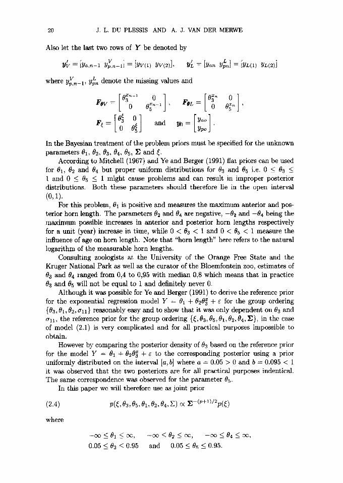
Also let the last two rows of Y be denoted by

= [ y o , n - 1 v

where y L Y~,n-1, Y~,~ denote the missing values and

o ' ' [oj o] F~ = 0~ and ~ = [ Ypo J "

In the Bayesian t reatment of the problem priors must be speeified for the unknown parameters 01, 02, 03, 04, 05, ~, and ~.

According to Mitchell (1967) and Ye and Berger (1991) flat priors can be used for 01, 02 and 04 but proper uniform distributions for 0a and 05 i.e. 0 _< 0~ _< 1 and 0 _< 05 _< 1 might cause problems and can result in improper posterior distributions. Both these parameters should therefore lie in the open interval (0, 1).

For this problem, 01 is positive and measures the maximum anterior and pos- terior horn length. The parameters 02 and 04 are negative, -02 and -04 being the maximum possible increases in anterior and posterior horn lengths respectively for a unit (year) increase in time, while 0 < 03 < 1 and 0 < ~ < 1 measure the influence of age on horn length. Note that "horn length" here refers to the natural logarithm of the measurable horn lengths.

Consulting zoologists at the University of the Orange Free State and the Kruger National Park as well as the curator of the Bloemfontein zoo, estimates of ~3 and 04 ranged from 0,4 to 0,95 with median 0,8 which means that in practice 0 3 and ~5 will not be equal to 1 and definitely never 0.

Although it was possible for Ye and Berger (1991) to derive the reference prior for the exponential regression model Y = 01 + 020~ + ~ for the group ordering {03, ~1,02, a11} reasonably easy and to show that it was only dependent on 03 and a11, the reference prior for the group ordering {~, 03, 03, 01,02, 04, E}, in the case of model (2.1) is very complicated and for all practical purposes impossible to obtain.

However by comparing the posterior density of 03 based on the reference prior for the model Y = ~1 + 020~ + ~ to the corresponding posterior using a prior uniformly distributed on the interval [a, b] where a = 0.05 > 0 and b = 0.095 < 1 it was observed that the two posteriors are for all practical purposes indentical. The same correspondence was observed for the parameter 05.

In this paper we will therefore use as joint prior

(2.4) p(~, 03, 05, 01,02, 04, E) 9(E-(P+I)/2p(~)

where

- c o _< 01 _< oc, - c o _< 02 <_ co, - c o _< 04 _< co,

0.05 _< 03 _< 0.95 and 0.05 < 03 _< 0.95.

BAYESIAN ESTIMATION: AGE OF RHINOCEROS 21

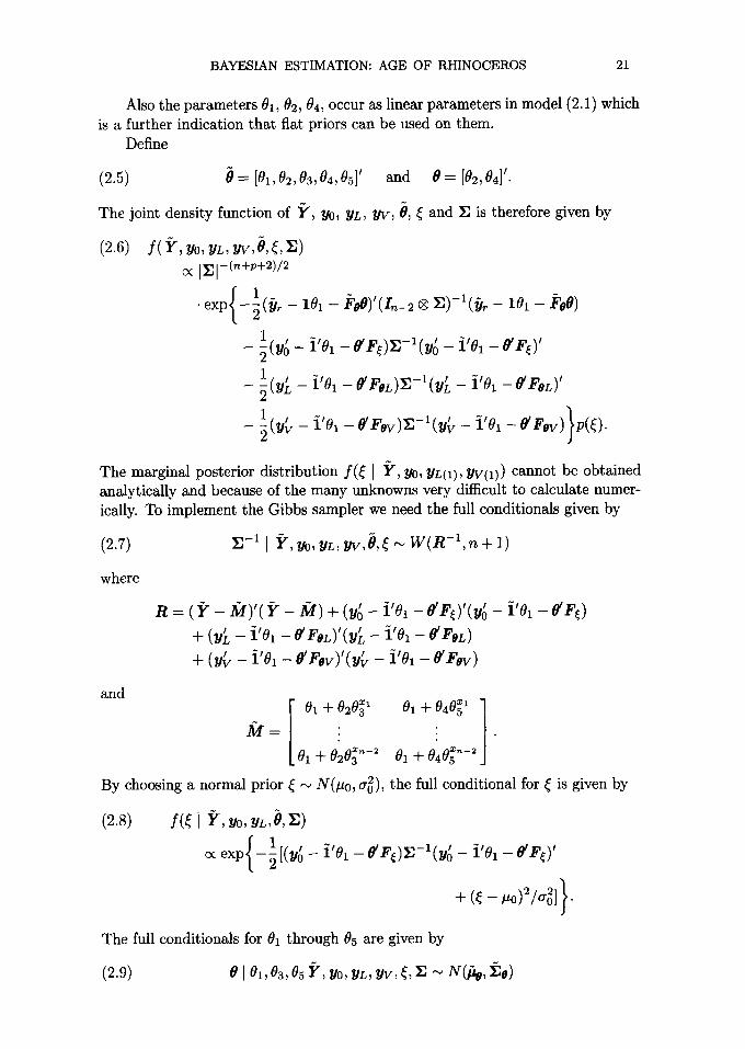
Also the parameters 91, ~2, 9a, occur as linear parameters in model (2.1) which is a further indication that flat priors can be used on them.

Define

(2.5) 0 = [91, 92, 93, 94, 95]' and 0 = [92, 94]'.

The joint density function of Y, Yo, YL, YV, 0, ~ and ~. is therefore given by

(2.6) f ( Y, Yo, YL, YV, 0, ~, ~])

IZJ-(~+P+2)/2

• exp - ~ ( ~ - l o l - ~'o0)'(x,~-2 ® r , ) - ~ ( ~ - lo~ - ~'~0)

1 ~ ~(~o - i'o1 - ¢ F ~ ) ~ - 1 ( ~ ; - i'01 - 0 ' F 0 '

1 ~ ~(~ - i'o1 - 0 ' F ~ ) S - I ( y ~ - i'0~ - O ' F ~ ) '

1 ¢ _

/ ~(~v i % - gF~v)~-~(~b - i % - CF~v)~p(~).

)

The marginal posterior distribution f(~ [ ~z, y0, YL(1), YV(1)) cannot be obtained analytically and because of the many unknowns very difficult to calculate numer- ically. To implement the Gibbs sampler we need the full conditionals given by

E-I I Y , Yo, YL, Uv,O,~~ W ( R - I , n + 1) (2.7)

where

R = ( i ~ - M ) ' ( i " - M ) + (y~ - i % - ¢ P 0 ' ( u ~ - i % - ¢ F ¢ )

+ (V'L - i % - CFeL)'(Y'L - i % -- C F 0 ~ )

+ (y~. - i'01 - f f F o v ) f ( y ~ , - i'91 - f f F a v )

and I 01 -]- 020~ 1 01 -[- 04{~ 1 ]

0 0 x~-: 01 + e4o~ ~-2 J 01-[- 23

By choosing a normal prior ~ -~ N(#o, a~), the full conditional for ~ is given by

(2.8) I ( ~ I i~, ~o, ~L, 0, r .)

~ exp - ~ [ ( ~ ; - i'ol - 0 ' F 0 r ~ - l ( y ; - i'01 - O'FO'

+ (~ - ~o)~/Oo ~] }-

The full conditionals for 01 through 05 are given by

(2.9) 0 ] 01,03, 05 Y, ~0, YL, ~h~V, ~, ~ ~ N(/@, ~]a)

22 J .L . DU PLESSIS AND A. J. VAN DER MERWE

where

and

--1 ! + F , Lr, (~L -- i 'el)' + F, v r , - l ( ~ - i'Ol)']

~# = [.~l'(In_ 2 (~ ~"~0' P q- F~]pa-IF~ + F,L~']-IF~L + F $ v ~ V ~ - l F ; v ] -

(2.10)

where

and

O~ [ 0,03,05, Y, Yo, YL, YV,{ , IB ~ N(f~o~,gr~)

+ i ' ~ - * ( y L -- CFSL) + i ' ~ - ' (~V -- ~'Fsv)]

a~, = [1'(I~_2 ® ~ ) - 1 1 + 3 i , ~ - 1 i ] - 1 .

(2.11)

(2.12)

f(03 ] 0,01,05, Y , ~ , yL, ~ , ~ , ~.)

oxp{ ® + (y~ - i % - ¢ F O r , - l ( y ~ - i % - e F t ) '

+ (~'L -- i % -- CFOL)r,-I(~'L -- i ' < -- ~FoL)'

+ ( ~ -- i % -- C F o v ) r , - i ( ~ b - i % - CFov) ' } I ,

f(05 I 0,01,e3, Y, yo, yL, YT,~, r~)

e x p { - ~ { ( ~ r - 101 - ~ ' ~ ) ' ( I n - 2 (~ ~ ' ~ * ) - l ( y r - 101 - F ~ ) O( %

+ ( ~ - i % - ¢ F e ) r , - l ( ~ - i'ol - e F t ) '

+ (y~ - i '01 - ¢FoL)E-~(y'L -- i'01 - gF, , , ) '

+ (yb - i'01 - ¢ F e v ) r , - l ( ~ ( ~ - i'01 - C F o v ) ' } ~ .

%

J

The condit ional densi ty for the missing value YL(2) is

(2.13)

where

YL(2) [ Y, Y0, YL(1), YV, 0, ~, ]E ~ N(E(yL(2)), Var(yL(2)))

E(YL(2)) ---- ~L(2) -{- 0 r 2 1 a l l 1 (YL(1) - - ~ L ( 1 ) )

and Var(yn(2)) = a22 - - 0"210"1110"12,

(see for example Anderson (1984)).

BAYESIAN ESTIMATION: AGE OF RHINOCEROS 23

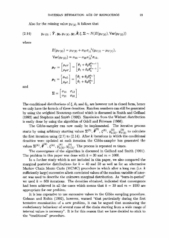
Also for the missing value YV(2) it follows that

(2.14) Yv(2) I Y , Yo, Yvo), YL, 0, 4, ~ "~ N(E(yv(2)), Var(Yv(2)))

where

and

E(yv(2)) = #v(2) + a~lal-)(Yv(1) - #v(1)),

Var(yy(2)) = a22 - o"21o"11 l a 1 2 ,

rlE-oo xn-1] # a V ~ O1 "-r 2 3

I'$V ---- I.[~pV J 01 d - 0 4 0 5 "~-~ '

~ L : l ]~pL j O1 -l- 040~ '~

La~l a22

The conditional distributions of 4, 03 and 05, are however not in closed form, hence we only have the kernels of these densities. Random numbers can still be generated by using the weighted Bootstrap method which is discussed in Smith and Gelfand (1992) and Stephens and Smith (1992). Simulation from the Wishart distribution is easily done by using the algorithm of Odell and Feiveson (1966).

The Gibbs-sampler can now easily be implemented. The iterative process

starts by using arbitrary starting values ]E (°), ~(0), 4(0) ' ~ (0) y(0) to calculate ~(2), v(2) the first iteration using (2.7) to (2.14). After k iterations in which the conditional densities were updated at each iteration the Gibbs-sampler has generated the

values ]E (k) 0(k), ~(k) ~ (k) ~ (k) , , ~L(2), uY(2)" The process is repeated m times.

The convergence of the algorithm is discussed in Gelfand and Smith (1991). The problem in this paper was done with k = 30 and m = 1000.

In a further study which is not included in this paper, we also compared the marginal posterior distributions for k = 40 and 50 as well as for an alternative Markov Chain Monte Carlo (MCMC) procedure in which after a long run (i.e. k sufficiently large) successive albeit correlated values of the random variable of inter- est was used to describe the unknown marginal distribution. As "burn-in-period" we used k = 500 iterations. The densities obtained, indicated that convergence had been achieved in all the cases which means that k = 30 and m = 1000 are appropriate for our problem.

It is less expensive to use successive values in the Gibbs sampling procedure. Gelman and Rubin (1992), however, warned "that particularly during the first tentative examination of a new problem, it can be argued that monitoring the evolutionary behaviour of several runs of the chain starting from a wide range of interval values is necessary". It is for this reason that we have decided to stick to the "traditional" procedure.

24 J. L. DU PLESSIS AND A. J. VAN DER MERWE

3. Example

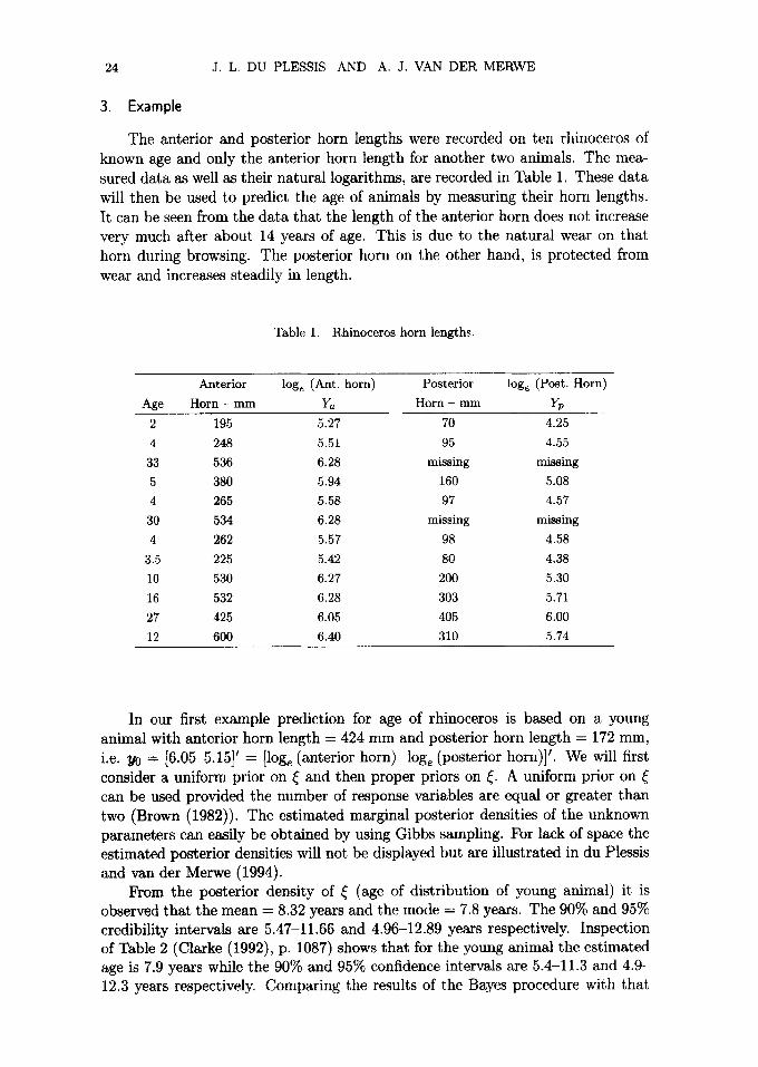
The anterior and posterior horn lengths were recorded on ten rhinoceros of known age and only the anterior horn length for another two animals. The mea- sured data as well as their natural logarithms, are recorded in Table 1. These data will then be used to predict the age of animals by measuring their horn lengths. It can be seen from the data that the length of the anterior horn does not increase very much after about 14 years of age. This is due to the natural wear on that horn during browsing. The posterior horn on the other hand, is protected from wear and increases steadily in length.

Table 1. Rhinoceros horn lengths.

Anterior log e (Ant. horn) Posterior log e (Post. Horn)

Age Horn - m m Ya Horn - m m Yp

2 195 5.27 70 4.25

4 248 5.51 95 4.55

33 536 6.28 missing missing

5 380 5.94 160 5.08

4 265 5.58 97 4.57

30 534 6.28 missing missing

4 262 5.57 98 4.58

3.5 225 5.42 80 4.38

10 530 6.27 200 5.30

16 532 6.28 303 5.71

27 425 6.05 405 6.00

12 600 6.40 310 5.74

In our first example prediction for age of rhinoceros is based on a young animal with anterior horn length = 424 mm and posterior horn length = 172 mm, i.e. Y0 = [6.05 5.15]' = [log e (anterior horn) log e (posterior horn)]'. We will first consider a uniform prior on ~ and then proper priors on ~. A uniform prior on can be used provided the number of response variables are equal or greater than two (Brown (1982)). The estimated marginal posterior densities of the unknown parameters can easily be obtained by using Gibbs sampling. For lack of space the estimated posterior densities will not be displayed but are illustrated in du Plessis and van der Merwe (1994).

From the posterior density of ~ (age of distribution of young animal) it is observed that the mean = 8.32 years and the mode = 7.8 years. The 90% and 95% credibility intervals are 5.47-11.66 and 4.96-12.89 years respectively. Inspection of Table 2 (Clarke (1992), p. 1087) shows that for the young animal the estimated age is 7.9 years while the 90% and 95% confidence intervals are 5.4-11.3 and 4.9- 12.3 years respectively. Comparing the results of the Bayes procedure with that

BAYESIAN ESTIMATION: AGE OF RHINOCEROS 25

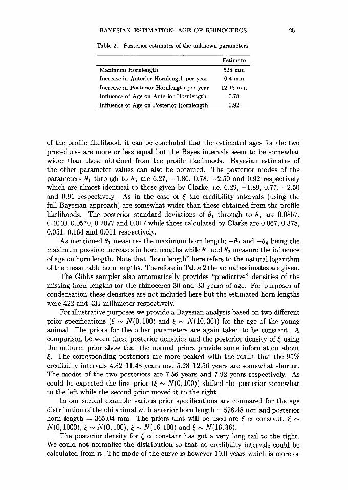
Table 2. Posterior estimates of the unknown parameters.

Estimate

Maximum Hornlength 528 mm

Increase in Anterior Hornlength per year 6.4 mm

Increase in Posterior Hornlength per year 12.18 mm

Influence of Age on Anterior Hornlength 0.78

Influence of Age on Posterior Hornlength 0.92

of the profile likelihood, it can be concluded that the estimated ages for the two procedures are more or less equal but the Bayes intervals seem to be somewhat wider than those obtained from the profile likelihoods. Bayesian estimates of the other parameter values can also be obtained. The posterior modes of the parameters 01 through to 0~ are 6.27, -1.86, 0.78, -2 .50 and 0.92 respectively which are almost identical to those given by Clarke, i.e. 6.29, -1.89, 0.77, -2 .50 and 0.91 respectively. As in the case of ~ the credibility intervals (using the full Bayesian approach) are somewhat wider than those obtained from the profile likelihoods. The posterior standard deviations of 01 through to 05 are 0.0857, 0.4040, 0.0570, 0.2077 and 0.017 while those calculated by Clarke are 0.067, 0.378, 0.051, 0.164 and 0.011 respectively.

As mentioned 81 measures the maximum horn length; -82 and -84 being the maximum possible increases in horn lengths while 81 and 83 measure the influence of age on horn length. Note that "horn length" here refers to the natural logarithm of the measurable horn lengths. Therefore in Table 2 the actual estimates are given.

The Gibbs sampler also automatically provides "predictive" densities of the missing horn lengths for the rhinoceros 30 and 33 years of age. For purposes of condensation these densities are not included here but the estimated horn lengths were 422 and 431 millimeter respectively.

For illustrative purposes we provide a Bayesian analysis based on two different prior specifications (~ ~ N(0, 100) and ~ ~ N(10, 36)) for the age of the young animal. The priors for the other parameters are again taken to be constant. A comparison between these posterior densities and the posterior density of ~ using the uniform prior show that the normal priors provide some information about ~. The corresponding posteriors are more peaked with the result that the 95% credibility intervals 4.82-11.48 years and 5.28-12.56 years are somewhat shorter. The modes of the two posteriors are 7.56 years and 7.92 years respectively. As could be expected the first prior (~ ~ N(0,100)) shifted the posterior somewhat to the left while the second prior moved it to the right.

In our second example various prior specifications are compared for the age distribution of the old animal with anterior horn length = 528.48 m m and posterior horn length = 365.04 mm. The priors that will be used are ~ o¢ constant, ~ N(0, 1000), ~ ~ N(0,100), ~ ~ N(16, 100) and ~ ~ N(16, 36).

The posterior density for ~ c< constant has got a very long tail to the right. We could not normalize the distribution so that no credibility intervals could be calculated from it. The mode of the curve is however 19.0 years which is more or

26 J. L. DU PLESSIS AND A. J. VAN DER MERWE

less the same as the estimated 19.2 years given by Clarke. For the second prior (~ ~ N(0, 1000)) the posterior mode is also 18.8 while the 95% credibility interval is 11.40-40.40 years. The corresponding 95% interval calculated from the profile likelihood is 12.8-31.7. The Bayes interval is again somewhat wider. The posterior modes for the remaining cases ~ ,-~ N(0, 100), ~ ~ N(16, 100) and ~ ~ N(t6, 36) are 16.4, 18.4 and 17.9 years respectively while the 95% credibility intervals are 10.62-24.11, 11.60-28.41 and 12.37-25.20 years respectively. For these three cases the 95% credibility intervals are somewhat shorter than the corresponding inter- vals given by Clarke. A comparison of the modes of the posterior densities and the lengths of the credibility intervals show that the priors provide substantial information about ~ for the old animal. For further details see du Plessis and van der Merwe (1994).

To accommodate the possibility of outlying rhinos the assumption of Gaussian errors will be relaxed in the direction of the Student-t family. Consider the series of independent errors ei I Z, A~ ~ N(0, )~i]E), (i = 1 , . . . , n). By placing a prior on ~ enables a wide variety of model error densities f(e~ I E) to emerge as scale mixtures of normal distributions (Andrews and Mallows (1974), Carlin and Polson (1991) and Wakefield et al. (1994)).

f(e~ I E )= /p (e i I :E,)~i)p()~i)dA~ (i = 1 , . . . , n ) .

For this example it is assumed that vA~ -1 ~ X~ so that ei I Z ~ t~(0, ]E), a multivariate Student-t-distribution with mean 0, covariance matrix ]E and degrees of freedom p. As in Wakefield et al. (1994) we will take v equal to 2.

The conditional posterior density of )~i will now be an Inverse Gamma density and the remaining hierarchical structure is defined exactly as in Section 2 except that Ai, (i = 1 , . . . , n) will occur in the expressions of the conditional densities defined in equations (2.7)-(2.14).

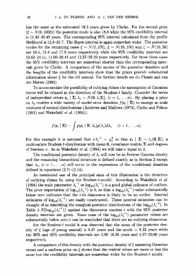
As mentioned one of the principal aims of this illustration is the detection of outlying rhinos by using the Student-t-model. According to Wakefield et al. (1994) the scale parameter ~-1 or lOgl0()~ -1) is a good global indicator of outliers. The prior expectation of logl0(),~ -1) is 0, so that a loglo()~-l)-value substantially below zero indicates that the i-th rhinoceros is likely to be an outlier. Interval estimates of logl0(,X~ 1) are easily constructed. These interval estimates can be thought of as describing the marginal posterior distributions of the logl0(A(1). In Table 3 E{logl0(A;-1)} against the rhinoceros number i with the 95% posterior density intervals axe given. Since none of the lOgl0(,k~ -1) parameter values are substantially below zero it can be concluded that there are no outlying rhinoceros.

For the Student-t model it was observed that the mean of the posterior den- sity of ~ (age of young animal) is 9.37 years and the mode = 8.22 years while the 90% and 95% credibility intervals are 5.60-16.38 years and 4.87-20.60 years respectively.

A comparison of this density with the posterior density of ~ assuming Gaussian errors and a uniform prior on ~ shows that the central values axe more or less the same but the credibility intervals are somewhat wider for the Student-t model.

Table 3.

BAYESIAN ESTIMATION: AGE OF RHINOCEROS

E{log10(A~-l)} against case number i with the 95% credibility interval.

Case Number i E{logl0(A~l)} 95%Credibi l i ty Interval

1 1.1002 -0.2245 - 4.2812

2 0.6097 -0.9116 - 2.1193

3 1.1650 -0.0180 - 4.3252

4 0.3986 -0.8465 - 2.1654

5 0.4329 -0.7886 - 2.6482

6 0.5523 -0.6418 - 2.6961

7 0.9471 -0.2963 - 3.8344

8 0.5577 -0.7014 - 2.5776

9 1.0632 -0.2261 - 4.0227

10 0.9949 -0.0594 - 3.8232

11 0.5663 -0.6863 - 3.0241

12 0.5715 -0.9517 - 3.0387

13 0.6415 -0.7914 - 2.8559

27

Table 4. Posterior est imates of ~, the age (years) of the two rhinoceros.

Mode 95% Credibility Interval

Young Animal - Uniform Prior 7.8

Young Animal - N(0, 100) Prior 7.56

Young Animal - N(10,36) Prior 7.92

Young Animal - Uniform Prior

Student- t Model 8.22

Old Animal - Uniform Prior 19.0

Old Animal - N(0, 1000) Prior 18.8

Old Animal - N(16, 36) Prior 17.9

Old Animal - N(0, 100) Prior 16.4

Old Animal - N(16, 100) Prior 18.4

4.96 - 12.89

4.82 - 11.48

5.28 - 12.56

4.87 - 20.60

11.40 - 40.40

12.37 - 25.20

10.62 - 24.11

11.60 - 28.41

I n T a b l e 4 p o s t e r i o r e s t i m a t e s o f t h e a g e d i s t r i b u t i o n s o f t h e t w o r h i n o c e r o s

a r e g i v e n . F o r f u r t h e r d e t a i l s a b o u t t h e p o s t e r i o r d e n s i t i e s s ee d u P l e s s i s a n d v a n

d e r M e r w e (1994) .

A c k n o w l e d g e m e n t s

T h e a u t h o r s w i s h t o e x p r e s s t h e i r g r a t i t u d e t o t h e r e f e r e e s a n d e d i t o r fo r t h e i r

h e l p f u l c o m m e n t s in r e v i s i n g t h e p a p e r .

R E F E R E N C E S

Anderson, T. W. (1984). An Introduction to Multivariate Statistical Analysis (2nd ed.), Wiley, New York.

28 J . L . DU PLESSIS AND A. J. VAN DEFt MERWE

Andrews, D. F. and Mallows, C. L. (1974). Scale mixtures of normality, J. Roy. Statist. Soc. Set. B, 36, 99-102.

Bates, D. M. and Watts, D. G. (1988). Nonlinear Regression Analysis and Its Applications, Wiley, New York.

Box, G. E. P. and Tiao, G. C. (1973). Bayesian Inference in Statistical Analysis, Addison Wesley, Massachusetts.

Brown, P. J. (1982). Multivariate calibration, J. Roy. Statist. Soc. Set. B, 46(3), 287-321. Carlin, B. P. and Poison, N. G. (1991). Inference for non conjugate Bayesian models using the

Gibbs sample, Canad. J. Statist., 19(4), 399-405. Carlin, B. P., Gelfand, A. E. and Smith, A. F. M. (1992). Hierarchical Bayes analysis of change

point problems, Applied Statistics, 41(2), 389-405. Clarke, G. P. Y. (1992). Inverse estimates from a multi-response model, Biometrics, 48(4),

1081-1094. du Plessis, J. L. and van der Merwe, A. J. (1994). An example of non linear Bayesian cal ibrat ion--

estimating the age of rhinoceros, Tech. Report No. 212, Department of Mathematical Statis- tics, University of the Orange Free State, South Africa.

Gelfand, A. E., Hills, S. E., Racine-Poon, A. and Smith, A. F. M. (1990). Illustration of Bayesian inference in normal data models using Gibbs sampling, J. Amer. Statist. Assoc., 85,972-985.

Gelfand, A. E. and Smith, A. F. M. (1991). Gibbs sampling for marginal posterior expections, Comm. Statist. Theory Methods, 20(5, 6) 1747-1766.

Gelfand, A. E.~ Smith, A. F. M. and Lee, T. M. (1992). Bayesian analysis of constrained parameters and truncated data problems using Gibbs sampling, J. Amer. Statist. Assoc., 87, 523-532.

Gelman, A. and Rubin, D. R. (1992). A single series from the Gibbs sampler provides a false sense of security, Bayesian Statistics 4 (ed. J. M. Bernardo, J. Berger, A. P. Dawid and A. F. M. Smith), 627~35, Oxford University Press, Oxford.

Geman, S. and Geman, D. (1984). Stochastic relaxation, Gibbs distributions, and the Bayesian restoration of images, IEEE Transactions on Pattern Analysis and Machine Intelligence, 6, 721-741.

Hastings, W. K. (1970). Monte Carlo sample methods using Markov chain and their applications, Biometrika, 57, 97-109.

Hunter, W. G. and Lamboy, W. F. (1981). A Bayesian analysis of the linear calibration problem, Technometrics, 23, 323-350.

Krutchkoff, R. C. (1967). Classical and inverse regression methods of calibration, Technometrics, 9, 425-439.

Mitchell, A. (1967). Discussion of paper by I. J. Good, J. R. Statist. Soc., B29, 423-424. Odell, P. L. and Feiveson, A. H. (1966). A numerical procedure to generate a sample covariance

matrix, J. Amer. Statist. Assoc., 61, 198-203. Oman, S. D. and Wax, Y. (1984). Estimating fetal age by ultrasound measurements: An example

of multivariate calibration, Biometrics, 40, 947-960. Scheff~, H. (1973). A statistical theory of calibration, Ann. Statist., 1, 1-37. Smith, A. F. M. and Gelfand, A. E. (1992). Bayesian statistics without tears: A sampling-

resampling perspective, Amer. Statist., 46(2), 84-88. Smith, R. L. and Corbett, M. (1987). Measuring marathon courses: An application of statistical

calibration~ Applied Statistics~ 36~ 283-295. Stephens, D. A. and Smith~ A. F. M. (1992). Sampling-resampling techniques for the computation

of posterior densities in normal means problems, Test, 1(1), 1-18. Wakefield, J. C., Smith, A. F. M., Racine-Poon, A. and Gelfand, A. E. (1994). Bayesian analysis

of linear and non-linear population models by using the Gibbs sampler, Applied Statistics, 43(1), 201-221.

Williams, E. J. (1969). A note on regression methods in calibration, Technometrics, 11,189-192. Ye, K. and Berger, J. O. (1991). Noninformative priors for inferences in exponential regression

models, Biometrika, 75(3), 645-656.