Embed Size (px)
Citation preview

Hindawi Publishing CorporationJournal of Probability and StatisticsVolume 2012, Article ID 617678, 26 pagesdoi:10.1155/2012/617678
Research ArticleBayesian Approach to Zero-InflatedBivariate Ordered Probit Regression Model, withan Application to Tobacco Use
Shiferaw Gurmu1 and Getachew A. Dagne2
1 Department of Economics, Andrew Young School of Policy Studies, Georgia State University,P.O. Box 3992, Atlanta, GA 30302, USA
2 Department of Epidemiology and Biostatistics, College of Public Health, University of South Florida,Tampa, FL 33612, USA
Correspondence should be addressed to Shiferaw Gurmu, [email protected]
Received 13 July 2011; Revised 18 September 2011; Accepted 2 October 2011
Academic Editor: Wenbin Lu
Copyright q 2012 S. Gurmu and G. A. Dagne. This is an open access article distributed underthe Creative Commons Attribution License, which permits unrestricted use, distribution, andreproduction in any medium, provided the original work is properly cited.
This paper presents a Bayesian analysis of bivariate ordered probit regression model with excessof zeros. Specifically, in the context of joint modeling of two ordered outcomes, we develop zero-inflated bivariate ordered probit model and carry out estimation usingMarkov ChainMonte Carlotechniques. Using household tobacco survey data with substantial proportion of zeros, we analyzethe socioeconomic determinants of individual problem of smoking and chewing tobacco. In ourillustration, we find strong evidence that accounting for excess zeros provides good fit to the data.The example shows that the use of a model that ignores zero-inflation masks differential effects ofcovariates on nonusers and users.
1. Introduction
This paper is concerned with joint modeling of two ordered data outcomes allowing forexcess zeros. Economic, biological, and social science studies often yield data on two orderedcategorical variables that are jointly dependent. Examples include the relationship betweendesired and excess fertility [1, 2], helmet use and motorcycle injuries [3], ownership of dogsand televisions [4], severity of diabetic retinopathy of the left and right eyes [5], and self-assessed health status and wealth [6]. The underlying response variables could be measuredon an ordinal scale. It is also common in the literature to generate a categorical or groupedvariable from an underlying quantitative variable and then use ordinal response regressionmodel (e.g., [4, 5, 7]). The ensuing model is usually analyzed using the bivariate orderedprobit model.

2 Journal of Probability and Statistics
Many ordered discrete data sets are characterized by excess of zeros, both in terms ofthe proportion of nonusers and relative to the basic ordered probit or logit model. The zerosmay be attributed to either corner solution to consumer optimization problem or errors inrecording. In the case of individual smoking behavior, for example, the zeros may be recordedfor individuals who never smoke cigarettes or for those who either used tobacco in the pastor are potential smokers. In the context of individual patents applied for by scientists duringa period of five years, zero patents may be recorded for scientists who either never madepatent applications or for those who do but not during the reporting period [8]. Ignoring thetwo types of zeros for nonusers or nonparticipants leads to model misspecification.
The univariate as well as bivariate zero-inflated count data models are well establishedin the literature for example, Lambert [9], Gurmu and Trivedi [10], Mullahy [11], and Gurmuand Elder [12]. The recent literature presents a Bayesian treatment of zero-inflated Poissonmodels in both cross-sectional and panel data settings (see [13, 14], and references there in).By contrast, little attention has been given to the problem of excess zeros in the ordereddiscrete choice models. Recently, an important paper by Harris and Zhao [15] developeda zero-inflated univariate ordered probit model. However, the problem of excess zeros inordered probit models has not been analyzed in the Bayesian framework. Despite recentapplications and advances in estimation of bivariate ordered probit models [1–6], we knowof no studies that model excess zeros in bivariate ordered probit models.
This paper presents a Bayesian analysis of bivariate ordered probit model with excessof zeros. Specifically, we develop a zero-inflated ordered probit model and carry out theanalysis using the Bayesian approach. The Bayesian analysis is carried out using MarkovChain Monte Carlo (MCMC) techniques to approximate the posterior distribution of theparameters. Bayesian analysis of the univariate zero-inflated ordered probit will be treatedas a special case of the zero-inflated bivariate order probit model. The proposed modelsare illustrated by analyzing the socioeconomic determinants of individual choice problemof bivariate ordered outcomes on smoking and chewing tobacco. We use household tobaccoprevalence survey data fromBangladesh. The observed proportion of zeros (those identifyingthemselves as nonusers of tobacco) is about 76% for smoking and 87% for chewing tobacco.
The proposed approach is useful for the analysis of ordinal data with natural zeros.The empirical analysis clearly shows the importance of accounting for excess zeros inordinal qualitative response models. Accounting for excess zeros provides good fit to thedata. In terms of both the signs and magnitudes of marginal effects, various covariateshave differential impacts on the probabilities associated with the two types of zeros,nonparticipants and zero-consumption. The usual analysis that ignores excess of zeros masksthese differential effects, by just focusing on observed zeros. The empirical results also showthe importance of taking into account the uncertainty in the parameter estimates. Anotheradvantage of the Bayesian approach to modeling excess zeros is the flexibility, particularlycomputational, of generalizing to multivariate ordered response models.
The rest of the paper is organized as follows. Section 2 describes the proposed zero-inflated bivariate probit model. Section 3 presents the MCMC algorithm and model selectionprocedure for the model. An illustrative application using household tobacco consumptiondata is given in Section 4. Section 5 concludes the paper.
2. Zero-Inflated Bivariate Ordered Probit Model
2.1. The Basic Model
We consider the basic Bayesian approach to a bivariate latent variable regression model withexcess of zeros. To develop notation, let y∗
1i and y∗2i denote the bivariate latent variables. We

Journal of Probability and Statistics 3
consider two observed ordered response variables y1i and y2i taking on values 0, 1, . . . , Jr ,for r = 1, 2. Define two sets of cut-off parameters αr = (αr2, αr3, . . . , αrJr), r = 1, 2, where therestrictions αr0 = −∞, αrJr+1 = ∞, and αr1 = 0 have been imposed. We assume that (y∗
1i, y∗2i)
′ ≡y∗i follows a bivariate regression model
y∗ri = x′riβr + εri, r = 1, 2, (2.1)
where xri is aKr-variate of regressors for the ith individual (i = 1, . . . ,N) and εri are the errorterms. For subsequent analysis, let β = (β′
1,β′2)
′, εi = (ε1i, ε2i)′, and
Xi =
(
x′1i 0′
0′ x′2i
)
. (2.2)
Analogous to the univariate case, the observed bivariate-dependent variables are defined as
yri =
⎧
⎪
⎪
⎪
⎪
⎪
⎪
⎪
⎨
⎪
⎪
⎪
⎪
⎪
⎪
⎪
⎩
0 if y∗ri ≤ 0,
1 if 0 < y∗ri ≤ αr2,
j if αrj < y∗ri ≤ αrj+1, j = 2, 3, . . . , Jr − 1,
Jr if y∗i ≤ αrJr ,
(2.3)
where r = 1, 2. Let yi = (y1i, y2i)′.
We introduce inflation at the point (y1i = 0, y2i = 0), called the zero-zero state. As inthe univariate case, define the participation model:
s∗i = z′iγ + μi,
si = I(
s∗i > 0)
.(2.4)
In the context of the zero-inflation model, the observed response random vector yi = (y1i, y2i)′
takes the form
yi = siyi. (2.5)
We observe yi = 0 when either the individual is a non-participant (si = 0) or the individualis a zero-consumption participant (si = 1 and yi = 0). Likewise, we observe positive outcome(consumption) when the individual is a positive consumption participant for at least onegood (si = 1 and yi /= 0).
Let Φ(a) and φ(a) denote the respective cumulative distribution and probabilitydensity functions of standardized normal evaluated at a. Assuming normality and that μi is

4 Journal of Probability and Statistics
uncorrelated with (ε1i, ε2i), but corr(ε1i, ε2i) = ρ12 /= 0, and each component with unit variance,the zero-inflated bivariate ordered probit (ZIBOP) distribution is
fb(
y∗i ,yi, s∗i , si | Xi, zi,Ψ
)
=
⎧
⎨
⎩
Pr(si = 0)+(1 − Pr(si = 0))Pr(
y1i = 0, y2i = 0)
, for(
y1i, y2i)
= (0, 0)
(1 − Pr(si = 0))Pr(
y1i = j, y2i = l)
, for(
y1i, y2i)
/= (0, 0),
(2.6)
where j = 0, 1, . . . , J1, l = 0, 1, . . . , J2, Pr(si = 0) = Φ(−z′iγ), Pr(si = 1) = Φ(−z′iγ). Further, for(y1i, y2i) = (0, 0) in (2.6), we have αr0 = −∞, αr1 = 0 for r = 1, 2 so that
Pr(
y1i = 0, y2i = 0)
= Φ2(−x′1iβ1,−x′2iβ2, ρ12
)
, (2.7)
where Φ2(·) is the cdf for the standardized bivariate normal. Likewise, Pr(y1i = j, y2i = l) in(2.6) are given by
Pr(
y1i = j, y2i = l)
= Φ2(
α1j+1 − x′1iβ1, α2l+1 − x′2iβ2; ρ12)
−Φ2(
α1j − x′1iβ1, α2l − x′2iβ2, ρ12)
for j = 1, . . . , J1 − 1; l = 1, . . . , J2 − 1;
Pr(
y1i = J1, y2i = J2)
= 1 −Φ2(
α1J1 − x′1iβ1, α2J2 − x′2iβ2, ρ12)
.
(2.8)
The ensuing likelihood contribution for N-independent observations is
Lb(y∗,y, s∗, s | X, z,Ψb) =N∏
i=1
∏
(j,l)=(0,0)
[
Pr(si = 0) + (1 − Pr(si = 0))Pr(
y1i = 0, y2i = 0)]dijl
×N∏
i=1
∏
(j,l)/= (0,0)
[
(1 − Pr(si = 0))Pr(
y1i = j, y2i = l)]dijl ,
(2.9)
where dijl = 1 if y1i = j and y2i = l, and dijl = 0 otherwise. Here, the vector Ψb consists ofβ, γ , α1, α2, and the parameters associated with the trivariate distribution of (ε, μ).
Regarding identification of the parameters in the model defined by (2.1) through(2.5) with normality assumption, we note that the mean parameter (joint choice probabilityassociate with the observed response vector yi) depends nonlinearly on the probabilityof zero inflation (Φ(−z′iγ)) and choice probability (Pr(y1i = j, y2i = l)) coming from theBOP submodel. Since the likelihood function for ZIBOP depends separately on the tworegression components, the parameters of ZIBOP model with covariates are identified aslong as the model is estimated by full maximum likelihood method. The same or differentsets of covariates can affect the two components via zi and xri. When using quasi-likelihoodestimation or generalized estimating equations methods rather than full ML, the class ofidentifiable zero-inflated count and ordered data models is generally more restricted; see, forexample, Hall and Shen [16] and references there in. Although the parameters in the ZIBOP

Journal of Probability and Statistics 5
model above are identified through a nonlinear functional form estimated by ML, for morerobust identification we can use traditional exclusion restrictions by including instrumentalvariables in the inflation equation, but excluding them from the ordered choice submodel.We follow this strategy in the empirical section.
About 2/3 of the observations in our tobacco application below have a double-zero-state, (y1 = 0, y2 = 0). Consequently, we focused on a mixture constructed from a point massat (0, 0) and a bivariate ordered probit. In addition to allowing for inflation in the double-zero-state, our approach can be extended to allow for zero-inflation in each component.
2.2. Marginal Effects
It is common to use marginal or partial effects to interpret covariate effects in nonlinearmodels; see, for example, Liu et al. [17]. Due to the nonlinearity in zero-inflated orderedresponse models and in addition to estimation of regression parameters, it is essential toobtain the marginal effects of changes in covariates on various probabilities of interest.These include the effects of covariates on probability of nonparticipation (zero-inflation),probability of participation, and joint and/or marginal probabilities of choice associated withdifferent levels of consumption.
From a practical point of view, we are less interested in the marginal effects ofexplanatory variables on the joint probabilities of choice from ZIBOP. Instead, we focus onthe marginal effects associated with the marginal distributions of yri for r = 1, 2. Define ageneric (scalar) covariate wi that can be a binary or approximately continuous variable. Weobtain themarginal effects of a generic covariatewi on various probabilities assuming that theregression results are based on ZIBOP. Ifwi is a binary regressor, then themarginal effect ofwi
on probability, say P , is the difference in the probability evaluated at 1 and 0, conditional onobservable values of covariates: P(wi = 1)−P(wi = 0). For continuous explanatory variables,the marginal effect is given by the partial derivative of the probability of interest with respectto wi, ∂P(·)/∂wi.
Regressor wi can be a common covariate in vectors of regressors xri and zi or appearsin either xri or zi. Focusing on the continuous regressor case, the marginal effects of wi ineach of the three cases are presented below. First, consider the case of common covariate inparticipation and main parts of the model, that is, wi in both xri and zi. The marginal effecton the probability of participation is given by
Mi(si = 1) =∂Pr(si = 1)
∂wi= φ(
z′iγ)
γwi , (2.10)
where again φ(·) is the probability density function (pdf) of the standard normal distributionand γwi is the coefficient in the inflation part associated with variablewi. In terms of the zeroscategory, the effect on the probability of nonparticipation (zero inflation) is
Mi(si = 0) =∂Pr(si = 0)
∂wi= −φ(−z′iγ
)
γwi , (2.11)

6 Journal of Probability and Statistics
while
Mi
(
s = 1, yri = 0)
=∂Pr(si = 1)Pr
(
yri = 0)
∂wi
= Φ(−x′riβr
)
φ(
z′iγ)
γwi −Φ(
z′iγ)
φ(−x′riβr
)
βrwi , r = 1, 2,
(2.12)
represents the marginal effect on the probability of zero-consumption. Here the scalar βrwi isthe coefficient in the main part of the model associated with wi.
Continuing with the case of common covariate, the marginal effects of wi on theprobabilities of choice are given as follows. First, the total marginal effect on the probability ofobserving zero-consumption is obtained as a sum of the marginal effects in (2.11) and (2.12);that is,
Mi
(
yri = 0)
=[
Φ(−x′riβr
) − 1]
φ(
z′iγ)
γwi −Φ(
z′iγ)
φ(−x′riβr
)
βrwi . (2.13)
The effects for the remaining choices for outcomes r = 1, 2 are as follows:
Mi
(
yri = 1)
=[
Φ(
αr2 − x′riβr
) −Φ(−x′riβr
)]
φ(
z′iγ)
γwi
−Φ(
z′iγ)[
φ(
αr2 − x′riβr
) − φ(−x′riβr
)]
βrwi ;
Mi
(
yri = j)
=[
Φ(
αr,j+1 − x′riβr
) −Φ(
αrj − x′riβr
)]
φ(
z′iγ)
γwi
−Φ(
z′iγ)[
φ(
αr,j+1 − x′riβr
) − φ(
αrj − x′riβr
)]
βrwi , for j = 2, . . . , Jr − 1;
Mi
(
yri = Jr)
=[
1 −Φ(
αr,Jr − x′riβr
)]
φ(
z′iγ)
γwi + Φ(
z′iγ)
φ(
αr,Jr − x′riβr
)
βrwi .
(2.14)
Now consider case 2, where a generic independent variable wi is included only in xri,the main part of the model. In this case, covariate wi has obviously no direct effect on theinflation part. The marginal effects of wi on various choice probabilities can be presented asfollows:
Mi
(
yri = j)
=∂Pr(
yri = j)
∂wi
= −Φ(z′iγ)[
φ(
αr,j+1 − x′riβr
) − φ(
αrj − x′riβr
)]
βrwi , for j = 0, 1, . . . , Jr ,
(2.15)
with αr0 = −∞, αr1 = 0, and αr,Jr+1 = ∞. The marginal effects in (2.15) can be obtained bysimply setting γwi = 0 in (2.13) and (2.14).
For case 3, where wi appears only in zi, its marginal effects on participationcomponents given in (2.10) and (2.11) will not change. Since βrwi = 0 in case 3, the partialeffects of wi on various choice probabilities take the form:
Mi
(
yri = j)
=[
Φ(
αr,j+1 − x′riβr
) −Φ(
αrj − x′riβr
)]
φ(
z′iγ)
γwi for j = 0, 1, . . . , Jr . (2.16)
Again, we impose the restrictions αr0 = −∞, αr1 = 0 and αr,Jr+1 = ∞.
Journal of Probability and Statistics 7
As noted by a referee, it is important to understand the sources of covariate effects andthe relationship between the marginal effects and the coefficient estimates. Since
Pr(
yri = j)
=[
Pr(si = 1)Pr(
yri = j)]
(2.17)
for j = 0, 1, . . . , Jr , the total effect of a generic covariate wi on probability of consumption atlevel j comes from two (weighted) sources: the participation part (Pr(si = 1)) and the mainordered probit part (Pr(yri = j)) such that
∂Pr(si = 1)∂wi
= φ(
z′iγ)
γwi ; (2.18)
∂Pr(
yri = j)
∂wi= −[φ(αr,j+1 − x′riβr
) − φ(
αrj − x′riβr
)]
βrwi(2.19)
with αr0 = −∞, αr1 = 0, s and αr,Jr+1 = ∞. This shows that sign(γwi) is the same as sign(∂Pr(si =1)/∂wi)—the participation effect in (2.18)—but sign(βrwi) is not necessarily the same as thesign of (∂Pr(yri = j)/∂wi). The latter is particularly true in the left tail of the distribution,where the coefficient (βrwi) and the main (unweighted) effect in (2.19) have opposite signsbecause
{−[φ(αr,j+1 − x′riβr
) − φ(
αrj − x′riβr
)]} ≡ (2.20)
is negative. In this case, a positive effect coming from the main part requires βrwi to benegative. By contrast, is positive in the right tail, but can be positive or negative when theterms (αr,j −x′riβr) and (αr,j+1−x′riβr) are on the opposite sides of the mode of the distribution.This shows that a given covariate can have opposite effects in the participation and mainmodels. Since the total effect of an explanatory variable on probability of choice is a weightedaverage of (2.18) and (2.19), interpretation of results should focus on marginal effects ofcovariates rather than the signs of estimated coefficients. This is the strategy adopted in theempirical analysis below.
2.3. A Special Case
Since the zero-inflated univariate ordered probit (ZIOP) model has not been analyzedpreviously in the Bayesian framework, we provide a brief sketch of the basic framework forZIOP. The univariate ordered probit model with excess of zeros can be obtained as a specialcase of the ZIBOP model presented previously. To achieve this, let ρ12 = 0 in the ZIBOPmodel and focus on the first ordered outcome with r = 1. In the standard ordered responseapproach, the model for the latent variable y∗
1i is given by (2.1) with r = 1. The observedordered variable y1i can be presented compactly as
y1i =J∑
j=0
jI(
α1j < y∗1i ≤ α1j+1
)
, (2.21)

8 Journal of Probability and Statistics
where I(w ∈ A) is the indicator function equal to 1 or 0 according to whether w ∈ A or not.Again α10, α11, . . . , α1J1 are unknown threshold parameters, where we set α10 = −∞, α11 = 0,and α1J1+1 = ∞.
Zero-inflation is now introduced at point y1i = 0. Using the latent variable model (2.4)for the zero inflation, the observed binary variable is given by si = I(s∗i > 0), where I(s∗i >0) = 1 if s∗i > 0, and 0 otherwise. In regime 1, si = 1 or s∗i > 0 for participants (e.g., smokers),while, in regime 0, si = 0 or s∗i ≤ 0 for nonparticipants. In the context of the zero-inflationmodel, the observed response variable takes the form y1i = siy1i. We observe y1i = 0 wheneither the individual is a non-participant (si = 0) or the individual is a zero-consumptionparticipant (si = 1 and y1i = 0). Likewise, we observe positive outcome (consumption) whenthe individual is a positive consumption participant (si = 1 and y∗
1i > 0).Assume that ε1 and μ are independently distributed. Harris and Zhao [15] also
consider the case where ε1 and μ are correlated. In the context of our application, thecorrelated model did not provide improvements over the uncorrelated ZIOP in termsof deviance information criterion. The zero-inflated ordered multinomial distribution, sayPr(y1i), arises as a mixture of a degenerate distribution at zero and the assumed distributionof the response variable y1i as follows:
f1(
y∗1i, y1i, s
∗i , si | x1i, zi,Ψ1
)
=
⎧
⎨
⎩
Pr(si = 0) + Pr(si = 1)Pr(
y1i = 0)
, for j = 0
Pr(si = 1)Pr(
y1i = j)
, for j = 1, 2, . . . , J1,(2.22)
where, for any parameter vector Ω10 associated with the distribution of (ε1, μ), Ψ1 =(β1, γ ,α
1,Ω10) with α1 = (α12, . . . , α1J1). For simplicity, dependence on latent variables,covariates, and parameters has been suppressed on the right-hand side of (2.22). Thelikelihood based on N-independent observations takes the form
L1(
y∗1, y1, s
∗, s | x1, z,Ψ1)
=N∏
i=1
J1∏
j=0
[
Pr(
y1i = j | x1i, zi,Ψ1)]dij
=N∏
i=1
∏
j=0
[
Pr(si = 0) + Pr(si = 1)Pr(
y1i = j)]dij
×N∏
i=1
∏
j>0
[
Pr(si = 1)Pr(
y1i = j)]dij ,
(2.23)
where, for example, y∗1 = (y∗
1, . . . , y∗N)′, and dij = 1 if individual i chooses outcome j, or dij = 0
otherwise.Different choices of the specification of the joint distribution of (ε1i, μi) give rise to
various zero-inflated ordered response models. For example, if the disturbance terms in thelatent variable equations are normally distributed, we get the zero-inflated ordered probitmodel of Harris and Zhao [15]. The zero-inflated ordered logit model can be obtained byassuming that ε1i and μi are independent, each of the random variables following the logisticdistribution with cumulative distribution function defined as Λ(a) = ea/(1 + ea). Unlike theordered probit framework, the ordered logit cannot lend itself easily to allow for correlation

Journal of Probability and Statistics 9
between bivariate discrete response outcomes. Henceforth, we focus on the ordered probitparadigm in both univariate and bivariate settings.
Assuming that ε1i and μi are independently normally distributed, each with mean 0and variance 1, the required components in (2.22) and consequently (2.23) are given by:
Pr(si = 0) = Φ(−z′iγ
)
,
Pr(
y1i = 0)
= Φ(−x′
1iβ1
)
,
Pr(
y1i = j)
= Φ(
α1j+1 − x′1iβ1
) −Φ(
α1j − x′1iβ1
)
, for j = 1, . . . , J1 − 1 with α10 = 0,
Pr(
y1i = J1)
= 1 −Φ(
α1J1 − x′1iβ1
)
.
(2.24)
The marginal effects for the univariate ZIOP are given by Harris and Zhao [15]. Bayesiananalysis of the univariate ZIOP will be treated as a special case of the zero-inflated bivariateorder probit model in the next section.
3. Bayesian Analysis
3.1. Prior Distributions
The Bayesian hierarchical model requires prior distributions for each parameter in the model.For this purpose, we can use noninformative conjugate priors. There are two reasons foradopting noninformative conjugate priors. First, we prefer to let the data dictate the inferenceabout the parameters with little or no influence from prior distributions. Secondly, thenoninformative priors facilitate resampling using Markov Chain Monte Carlo algorithm(MCMC) and have nice convergence properties. We assume noninformative (vague ordiffuse) normal priors for regression coefficients β, with mean β∗ and variance Ωβ whichare chosen to make the distribution proper but diffuse with large variances. Similarly, γ ∼N(γ∗,Ωγ).
In choosing prior distributions for the threshold parameters, α’s, caution is neededbecause of the order restriction on them. One way to avoid the order restriction is toreparameterize them. Following Chib and Hamilton [18] treatment in the univariate orderedprobit case, we reparameterize the ordered threshold parameters
τr2 = log(αr2); τrj = log(
αrj − αrj−1)
, j = 3, . . . , Jr ; r = 1, 2 (3.1)
with the inverse map
αrj =j∑
m=2
exp(τrm), j = 2, . . . , Jr ; r = 1, 2. (3.2)
For r = 1, 2, let τ r = (τr2, τr3, . . . , τrJ)′ so that τ = (τ1, τ2). We choose normal prior τ ∼
N(τ∗,Ωτ) without order restrictions for τr ’s.The only unknown parameter associate with the distribution of (ε, μ) in (2.1) and (2.4)
is ρ12, the correlation between ε1 and ε2. The values of ρ12 by definition are restricted to be in

10 Journal of Probability and Statistics
the −1 to 1 interval. Therefore, the choice for prior distribution for ρ12 can be uniform (−1, 1)or a proper distribution based on reparameterization. Let ν denote the hyperbolic arc-tangenttransformation of ρ12, that is,
ν = a tanh(
ρ12)
, (3.3)
and taking hyperbolic tangent transformation of ν gives us back ρ12 = tanh(ν). Thenparameter ν is asymptotically normal distributed with stabilized variance, 1/(N − 3), whereN is the sample size. We may also assume that ν ∼ N(ν∗, σ2
ν).
3.2. Bayesian Analysis via MCMC
For carrying out a Bayesian inference, the joint posterior distribution of the parameters ofthe ZIBOP model in (2.6) conditional on the data is obtained by combining the likelihoodfunction given in (2.9) and the above-specified prior distributions via Bayes’ theorem, as:
f(Ψb | x, z) ∝N∏
i=1
∏
(j,l)=(0,0)
[
Φ(−z′iγ
)
+ Φ(
z′iγ)
Φ2(−x′1iβ1,−x′2iβ2, ρ12
)]dijl
×N∏
i=1
∏
(j,l)/= (0,0)
[
Φ(
z′iγ)[
Φ2(
α1j+1 − x′1iβ1, α2l+1 − x′2iβ2; ρ12)
−Φ2(
α1j − x′1iβ1, α2l − x′2iβ2, ρ12)]
]dijl
× f(Ψb),(3.4)
where f(Ψb) ∝ f(β)f(γ)f(τ)f(ν) and the parameter vector Ψb now consists of β = (β′1,β
′2)
′,γ , τ = (τ1, τ2), s and ν = a tanh(ρ12). Here f(β) ∝ |Ωβ|−1/2 exp{−1/2(β − β∗)′Ω−1
β(β −
β∗)};f(γ) ∝ |Ωγ |−1/2 exp{−1/2(γ − γ ∗)′Ω−1γ (γ − γ ∗)};f(τ) ∝ |Ωτ |−1/2 exp{−1/2(τ − τ∗)′Ω−1
τ (τ −τ∗)};τrj are defined in (3.1), and αrj are given via the inverse map (3.2).
Full conditional posterior distributions are required to implement the MCMCalgorithm [19–22], and they are given as follows:
(1) fixed effects:
(a) zero state:
f(
γ | x, z,Ψ−γ) ∝ ∣∣Ωγ
∣
∣
−1/2 exp{
−12(γ − γ ∗)′Ω−1
γ (γ − γ ∗)}
× f(Ψb | x, z); (3.5)
(b) nonzero state:
f(
β | x, z,Ψ−β) ∝ ∣∣Ωβ
∣
∣
−1/2 exp{
−12(
β − β∗)′Ω−1β
(
β − β∗)}
× f(Ψb | x, z). (3.6)

Journal of Probability and Statistics 11
(2) thresholds:
f(τ | x, z,Ψ−τ) ∝ |Ωτ |−1/2 exp{
−12(τ − τ∗)′Ω−1
τ (τ − τ∗)}
×N∏
i=1
∏
(j,l)/= (0,0)
[
Φ(
z′iγ)[
Φ2(
α1j+1 − x′1iβ1, α2l+1 − x′2iβ2; ρ12)
−Φ2(
α1j − x′1iβ1, α2l − x′2iβ2, ρ12)]
]dijl
.
(3.7)
(3) bivariate correlation:
f(ν | x, z,Ψ−ν) ∝ σ−1ν exp
{
− (ν − ν∗)2
2σ2ν
}
× f(Ψb | x, z). (3.8)
The MCMC algorithm simulates direct draws from the above full conditionalsiteratively until convergence is achieved. A single long chain [23, 24] is used for the proposedmodel. Geyer [23] argues that using a single longer chain is better than using a number ofsmaller chains with different initial values. We follow this strategy in our empirical analysis.
The Bayesian analysis of the univariate ZIOP follows as a special case of that of theZIBOP presented above. In particular, the joint posterior distribution of the parameters ofthe ZIOP model in (2.22) conditional on the data is obtained by combining the likelihoodfunction given in (2.23) and the above-specified prior distributions (with modified notations)via Bayes’ theorem, as follows:
f(Ψ | x, z, ) ∝N∏
i=1
∏
j=0
[
Φ(−z′iγ
)
+ Φ(
z′iγ)
Φ(−x′iβ
)]dij
×N∏
i=1
∏
j>0
[
Φ(
z′iγ){
Φ(
αj+1 − x′iβ) −Φ
(
αj − x′iβ)}]dij
× f(β)f(γ)f(τ),
(3.9)
where, using notation of Section 2.3 for β and the other parameter vectors, f(β) ∝|Ωβ|−1/2 exp{−1/2(β −β∗)′Ω−1
β (β −β∗)}; f(γ) ∝ |Ωγ |−1/2 exp{−1/2(γ − γ ∗)′Ω−1γ (γ − γ ∗)}; f(τ) ∝
|Ωτ |−1/2 exp{−1/2(τ −τ∗)′Ω−1τ (τ −τ∗)}, τ2 = log(α2) and τj = log(αj −αj−1), j = 3, . . . , J . Apart
from dropping the bivariate correlation, we basically replace the bivariate normal cumulativedistribution Φ2(·, ·; ρ12) by the univariate counterpart Φ(·). Details are available upon requestfrom the authors.
Apart from Bayesian estimation of the regression parameters, the posterior distribu-tions of other quantities of interest can be obtained. These include posteriors for marginaleffects and probabilities for nonparticipation, zero-consumption, and joint outcomes ofinterest. These will be considered in the application section. Next, we summarize modelselection procedure.
The commonly used criteria for model selection like BIC and AIC are not appropriatefor the multilevel models (in the presence of random effects), which complicates the counting
12 Journal of Probability and Statistics
of the true number of free parameters. To overcome such a hurdle, Spiegelhalter et al. [25]proposed a Bayesian model comparison criterion, called Deviance Information Criterion(DIC). It is given as
DIC = goodness-of-fit + penalty for complexity, (3.10)
where the “goodness-of-fit” is measured by the deviance for θ = (β, γ, α)
D(θ) = −2 logL(data | θ) (3.11)
and complexity is measured by the “effective number of parameters”:
pD = Eθ|y[D(θ)] −D(
Eθ|y[θ])
= D −D(
θ)
;(3.12)
that is, posterior mean deviance minus deviance evaluated at the posterior mean of theparameters. The DIC is then defined analogously to AIC as
DIC = D(
θ)
+ 2pD
= D + pD.
(3.13)
The idea here is that models with smaller DIC should be preferred to models with larger DIC.Models are penalized both by the value ofD, which favors a good fit, but also (similar to AICand BIC) by the effective number of parameters pD. The advantage of DIC over other criteria,for Bayesian model selection, is that the DIC is easily calculated from the MCMC samples. Incontrast, AIC and BIC require calculating the likelihood at its maximum values, which arenot easily available from the MCMC simulation.
4. Application
4.1. Data
We consider an application to tobacco consumption behavior of individuals based on the 2001household Tobacco Prevalence survey data from Bangladesh. The Survey was conducted intwo administrative districts of paramount interest for tobacco production and consumptionin the country. Data on daily consumption of smoking and chewing tobacco along with othersocioeconomic and demographic characteristics and parental tobacco consumption habitswere collected from respondents of 10 years of age and above. The data set has been usedpreviously by Gurmu and Yunus [26] in the context of binary response models. Here wefocus on a sample consisting of 6000 individual respondents aged between 10 and 101 years.
The ordinal outcomes yr = 0, 1, 2, 3 used in this paper correspond roughly to zero,low, moderate, and high levels of tobacco consumption in the form of smoking (y1) orchewing tobacco (y2), respectively. The first dependent variable y1 for an individual’s daily
Journal of Probability and Statistics 13
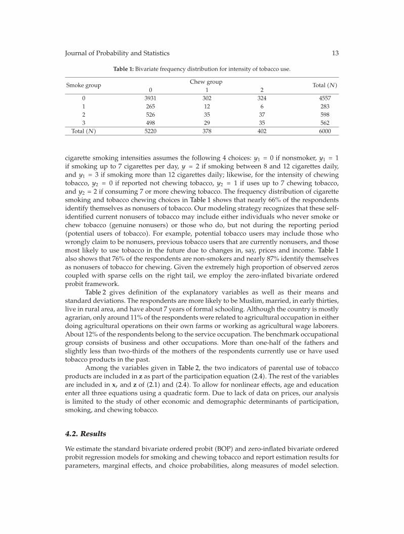
Table 1: Bivariate frequency distribution for intensity of tobacco use.
Smoke group Chew group Total (N)0 1 2
0 3931 302 324 45571 265 12 6 2832 526 35 37 5983 498 29 35 562
Total (N) 5220 378 402 6000
cigarette smoking intensities assumes the following 4 choices: y1 = 0 if nonsmoker, y1 = 1if smoking up to 7 cigarettes per day, y = 2 if smoking between 8 and 12 cigarettes daily,and y1 = 3 if smoking more than 12 cigarettes daily; likewise, for the intensity of chewingtobacco, y2 = 0 if reported not chewing tobacco, y2 = 1 if uses up to 7 chewing tobacco,and y2 = 2 if consuming 7 or more chewing tobacco. The frequency distribution of cigarettesmoking and tobacco chewing choices in Table 1 shows that nearly 66% of the respondentsidentify themselves as nonusers of tobacco. Our modeling strategy recognizes that these self-identified current nonusers of tobacco may include either individuals who never smoke orchew tobacco (genuine nonusers) or those who do, but not during the reporting period(potential users of tobacco). For example, potential tobacco users may include those whowrongly claim to be nonusers, previous tobacco users that are currently nonusers, and thosemost likely to use tobacco in the future due to changes in, say, prices and income. Table 1also shows that 76% of the respondents are non-smokers and nearly 87% identify themselvesas nonusers of tobacco for chewing. Given the extremely high proportion of observed zeroscoupled with sparse cells on the right tail, we employ the zero-inflated bivariate orderedprobit framework.
Table 2 gives definition of the explanatory variables as well as their means andstandard deviations. The respondents are more likely to be Muslim, married, in early thirties,live in rural area, and have about 7 years of formal schooling. Although the country is mostlyagrarian, only around 11% of the respondents were related to agricultural occupation in eitherdoing agricultural operations on their own farms or working as agricultural wage laborers.About 12% of the respondents belong to the service occupation. The benchmark occupationalgroup consists of business and other occupations. More than one-half of the fathers andslightly less than two-thirds of the mothers of the respondents currently use or have usedtobacco products in the past.
Among the variables given in Table 2, the two indicators of parental use of tobaccoproducts are included in z as part of the participation equation (2.4). The rest of the variablesare included in xr and z of (2.1) and (2.4). To allow for nonlinear effects, age and educationenter all three equations using a quadratic form. Due to lack of data on prices, our analysisis limited to the study of other economic and demographic determinants of participation,smoking, and chewing tobacco.
4.2. Results
We estimate the standard bivariate ordered probit (BOP) and zero-inflated bivariate orderedprobit regression models for smoking and chewing tobacco and report estimation results forparameters, marginal effects, and choice probabilities, along measures of model selection.

14 Journal of Probability and Statistics
Table 2: Definition and summary statistics for independent variables.
Name Definition Meanb St. Dev.
Agea Age in years 30.35 (14.9)
Educationa Number of years of formalschooling 6.83 (4.7)
Income Monthly family income in1000s of Taka 7.57 (10.3)
Male = 1 if male 54.6Married = 1 if married 57.2Muslim = 1 if religion is Islam 78.4Father use = 1 if father uses tobacco 54.0Mother use = 1 if mother uses tobacco 65.1
Region = 1 if Rangpur resident,= 0 if Chittagong resident 49.7
Urban = 1 if urban resident 38.0
Agriservice = 1 if agriculture labor orservice occupation 23.2
Self-employed = 1 if self-employed orhousehold chores 30.7
Student = 1 if student 26.8
Other = 1 if business or otheroccupations (control) 19.3
aIn implementation, we also include age squared and education squared.
bThe means for binary variables are in percentage.
Table 3: Goodness-of-fit statistics via DIC.
Model Dbar Dhat pD DICBivariate orderedprobit (BOP) 11417.1 11386.9 30.1 11447.2
Zero-inflated BOP 11301.1 11270.3 29.8 11329.9Dbar: Posterior mean of deviance, Dhat: Deviance evaluated at the posterior mean of the parameters, pD: Dbar-Dhat, theeffective number of parameters, and DIC: Deviance information criterion.
An earlier version of this paper reports results from the standard ordered probit model aswell as the uncorrelated and correlated versions of the univariate zero-inflated ordered probitmodel for smoking tobacco. Convergence of the generated samples is assessed using standardtools (such as trace plots and ACF plots) within WinBUGS software. After initial 10,000burn-in iterations, every 10th MCMC sample thereafter was retained from the next 100,000iterations, obtaining 10,000 samples for subsequent posterior inference of the unknownparameters. The slowest convergence is observed for some parameters in the inflationsubmodel. By contrast, the autocorrelations functions for most of the marginal effects dieout quickly relative to those for the associated parameters.
Table 3 reports the goodness-of-fit statistics for the standard bivariate ordered probitmodel and its zero-inflated version, ZIBOP. The ZIBOP regression model clearly dominatesBOP in terms of DIC and its components; compare the DIC of 11330 for the former and 11447for the latter model. Table 4 gives posterior means, standard deviations, medians, and the95 percent credible intervals (in terms of the 2.5 and 97.5 percentiles) of the parameters andchoice probabilities from ZIBOPmodel. For comparison, the corresponding results from BOP

Journal of Probability and Statistics 15
Table 4: Posterior mean, standard deviation, and 95% credible intervals of parameters from zibop forsmoking and chewing tobacco.
Variable Mean St. dev. 2.50% Median 97.50%
Main (β1,α1): smoking (y1):Age/10 0.672 0.119 0.444 0.685 0.894Age square/100 −0.070 0.012 −0.093 −0.071 −0.046Education −0.071 0.014 −0.097 −0.071 −0.042Education square 0.001 0.001 −0.002 0.001 0.003Income 0.000 0.002 −0.005 0.000 0.005Male 2.092 0.086 1.925 2.091 2.269Married 0.213 0.070 0.074 0.213 0.353Muslim −0.053 0.052 −0.157 −0.053 0.049Region −0.007 0.048 −0.102 −0.007 0.086Urban −0.096 0.051 −0.198 −0.097 0.004Agriservice −0.234 0.056 −0.345 −0.233 −0.125Self-employed −0.246 0.087 −0.414 −0.247 −0.069student −0.476 0.137 −0.742 −0.478 −0.204α12 0.284 0.017 0.252 0.283 0.318α13 0.987 0.030 0.928 0.987 1.048Main (β2,α2): chewing (y2)Age/10 0.649 0.133 0.382 0.658 0.893Age square/100 −0.046 0.013 −0.071 −0.046 −0.019Education −0.020 0.016 −0.052 −0.020 0.012Education square −0.002 0.001 −0.005 −0.002 0.000Income 0.001 0.003 −0.004 0.002 0.007Male −0.479 0.081 −0.641 −0.479 −0.320Married −0.025 0.075 −0.171 −0.025 0.122Muslim −0.072 0.056 −0.181 −0.072 0.039Region 0.417 0.051 0.317 0.418 0.517Urban −0.080 0.058 −0.194 −0.079 0.035Agriservice 0.052 0.074 −0.096 0.052 0.194Self-employed 0.127 0.092 −0.058 0.126 0.309Student −0.450 0.221 −0.887 −0.448 −0.023α22 0.484 0.023 0.439 0.484 0.531Inflation (γ):Age/10 −0.012 2.044 −4.755 0.253 2.861Age square/100 0.509 0.552 −0.197 0.398 1.812Education −0.218 0.115 −0.476 −0.204 −0.024Education square 0.028 0.011 0.010 0.026 0.053Income 0.006 0.022 −0.027 0.003 0.059Male 0.239 0.827 −1.582 0.417 1.379Married 2.306 4.478 −0.416 0.500 16.900Muslim −0.528 0.356 −1.331 −0.494 0.068Mother −0.170 0.267 −0.716 −0.164 0.345Father −0.119 0.330 −0.664 −0.160 0.605Region 0.630 0.291 0.061 0.625 1.222

16 Journal of Probability and Statistics
Table 4: Continued.
Variable Mean St. dev. 2.50% Median 97.50%
Urban 0.040 0.357 −0.737 0.071 0.675Agrservice 5.312 5.416 1.017 2.674 20.470Self-employed 3.783 5.025 0.124 1.275 17.990Sstudent −0.344 0.411 −1.154 −0.339 0.466ρ12 −0.185 0.033 −0.249 −0.186 −0.119Select probabilities:P (y1 = 0) 0.760 0.004 0.752 0.760 0.768P (y2 = 0) 0.871 0.004 0.864 0.871 0.879P (y1 = 0, y2 = 0) 0.662 0.005 0.652 0.662 0.671P (zero-inflation) 0.242 0.048 0.151 0.243 0.323Results for the constant terms in the main and inflation parts have been suppressed for brevity.
are shown in Table 6 of the appendix. Both models predict significant negative correlationbetween the likelihood of smoking and chewing tobacco. The posterior estimates of the cut-off points are qualitatively similar across models. In what follows, we focus on discussionof results from the preferred ZIBOP model. The 95% credible interval for the correlationparameter ρ12 from the zero-inflated model is in the range −0.25 to −0.12, indicating thatsmoking and chewing tobacco are generally substitutes. Results of selected predicted choiceprobabilities (bottom of Table 4) show that the ZIBOP regression model provides very goodfit to the data. The posterior mean for the probability of (zero, zero)-inflation is about 24%while the 95% credible interval is [0.15, 0.32], indicating that a substantial proportion of zerosmay be attributed to nonparticipants. These results underscore the importance of modelingexcess zeros in bivariate ordered probit models.
To facilitate interpretation of results, we report in Tables 5 and 7 the same set ofposterior estimates for the marginal effects from ZIBOP and BOP models, respectively.Since age and education enter the three equations non-linearly, we report the total marginaleffects coming from the linear and quadratic parts. We examine closely the marginal effectson the unconditional marginal probabilities at all levels of smoking and chewing tobacco(y1 = 0, 1, 2, 3; y2 = 0, 1, 2). The marginal effects reported in Table 5 show that the results forcovariates are generally plausible. Age has a negative impact on probabilities of moderateand heavy use of tobacco. For heavy smokers, education has a significant negative impact onthe probability of smoking cigarettes. An additional year of schooling on average decreasesprobability of smoking by about 6.9% for heavy smokers. Among participants, being male ormarried has positive impact on probability of smoking, while the effects for being Muslim,urban resident, and student are largely negative. Male respondents are more likely to smokecigarettes while women respondents are more likely to use chewing tobacco with heavyintensity, a result which is in line with custom of the country [26].
Using (2.13), we decompose the marginal effect on probability of observing zero-consumption into two components: the effect on nonparticipation (zero inflation) and zero-consumption. For each explanatory variable, this decomposition is shown in Table 5 in thefirst three rows for smoking and in rows 1, 7, and 8 for chewing tobacco. For most variables,the effects on probabilities of nonparticipation and zero-consumption are on average oppositein sign, but this difference seems to diminish at the upper tail of the distribution. For example,looking at the posterior mean for age under smoking, getting older by one more year

Journal of Probability and Statistics 17
Table 5: Posterior mean, standard deviation, and 95% credible intervals of marginal effects of covariateson probability of smoking and chewing tobacco (ZIBOP model).
Variable Probability Mean St. dev. 2.50% Median 97.50%
Age Nonparticipation −0.0259 0.0129 −0.0556 −0.0236 −0.0078Zero-consumption, y1 0.0463 0.0102 0.0294 0.0453 0.0687
All zeros, y1 = 0 0.0204 0.0059 0.0078 0.0213 0.0304y1 = 1 0.0058 0.0035 0.0009 0.0053 0.0138y1 = 2 −0.0014 0.0029 −0.0057 −0.0019 0.0055y1 = 3 −0.0690 0.0235 −0.1223 −0.0658 −0.0344
Zero-consumption, y2 0.0403 0.0116 0.0195 0.0386 0.0675All zeros, y2 = 0 0.0145 0.0064 0.0018 0.0149 0.0264
y2 = 1 −0.0034 0.0021 −0.0071 −0.0035 0.0008y2 = 2 −0.0019 0.0014 −0.0043 −0.0020 0.0011
Education Nonparticipation −0.2823 0.0768 −0.4260 −0.2837 −0.1252Zero-consumption, y1 0.2447 0.0749 0.0917 0.2459 0.3851
All zeros, y1 = 0 −0.0377 0.0241 −0.0853 −0.0374 0.0094y1 = 1 0.0498 0.0141 0.0231 0.0494 0.0789y1 = 2 0.0241 0.0102 0.0045 0.0239 0.0444y1 = 3 −0.5557 0.1536 −0.8415 −0.5588 −0.2417
Zero-consumption, y2 0.3136 0.0772 0.1561 0.3159 0.4546All zeros, y2 = 0 0.0313 0.0161 −0.0009 0.0315 0.0618
y2 = 1 −0.0134 0.0080 −0.0288 −0.0135 0.0027y2 = 2 −0.0222 0.0119 −0.0455 −0.0221 0.0009
Income Nonparticipation −0.0004 0.0015 −0.0038 −0.0002 0.0022Zero-consumption, y1 0.0003 0.0014 −0.0022 0.0002 0.0035
All zeros, y1 = 0 −0.0001 0.0004 −0.0009 −0.0001 0.0008y1 = 1 0.0001 0.0003 −0.0005 0.0000 0.0008y1 = 2 0.0000 0.0002 −0.0003 0.0000 0.0004y1 = 3 −0.0007 0.0030 −0.0075 −0.0004 0.0044
Zero-consumption, y2 0.0001 0.0016 −0.0025 0.0000 0.0036All zeros, y2 = 0 −0.0002 0.0005 −0.0011 −0.0002 0.0007
y2 = 1 0.0001 0.0002 −0.0003 0.0001 0.0004y2 = 2 0.0001 0.0001 −0.0002 0.0001 0.0003
Male Nonparticipation −0.0254 0.0599 −0.1268 −0.0305 0.1012Zero-consumption, y1 −0.3595 0.0611 −0.4900 −0.3540 −0.2565
All zeros, y1 = 0 −0.3849 0.0116 −0.4078 −0.3849 −0.3618y1 = 1 0.0630 0.0040 0.0555 0.0630 0.0711y1 = 2 0.1560 0.0065 0.1435 0.1559 0.1689y1 = 3 0.1659 0.0083 0.1503 0.1657 0.1829
Zero-consumption, y2 0.1012 0.0623 −0.0309 0.1064 0.2075All zeros, y2 = 0 0.0758 0.0126 0.0511 0.0759 0.1004
y2 = 1 0.0501 0.0033 0.0438 0.0500 0.0567y2 = 2 −0.1258 0.0112 −0.1478 −0.1258 −0.1040
Married Nonparticipation −0.0680 0.0777 −0.2274 −0.0433 0.0346Zero-consumption, y1 0.0200 0.0705 −0.0778 −0.0001 0.1692
All zeros, y1 = 0 −0.0480 0.0149 −0.0796 −0.0472 −0.0207
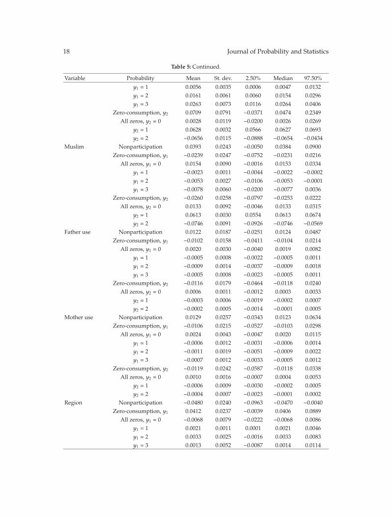
18 Journal of Probability and Statistics
Table 5: Continued.
Variable Probability Mean St. dev. 2.50% Median 97.50%
y1 = 1 0.0056 0.0035 0.0006 0.0047 0.0132y1 = 2 0.0161 0.0061 0.0060 0.0154 0.0296y1 = 3 0.0263 0.0073 0.0116 0.0264 0.0406
Zero-consumption, y2 0.0709 0.0791 −0.0371 0.0474 0.2349All zeros, y2 = 0 0.0028 0.0119 −0.0200 0.0026 0.0269
y2 = 1 0.0628 0.0032 0.0566 0.0627 0.0693y2 = 2 −0.0656 0.0115 −0.0888 −0.0654 −0.0434
Muslim Nonparticipation 0.0393 0.0243 −0.0050 0.0384 0.0900Zero-consumption, y1 −0.0239 0.0247 −0.0752 −0.0231 0.0216
All zeros, y1 = 0 0.0154 0.0090 −0.0016 0.0153 0.0334y1 = 1 −0.0023 0.0011 −0.0044 −0.0022 −0.0002y1 = 2 −0.0053 0.0027 −0.0106 −0.0053 −0.0001y1 = 3 −0.0078 0.0060 −0.0200 −0.0077 0.0036
Zero-consumption, y2 −0.0260 0.0258 −0.0797 −0.0253 0.0222All zeros, y2 = 0 0.0133 0.0092 −0.0046 0.0133 0.0315
y2 = 1 0.0613 0.0030 0.0554 0.0613 0.0674y2 = 2 −0.0746 0.0091 −0.0926 −0.0746 −0.0569
Father use Nonparticipation 0.0122 0.0187 −0.0251 0.0124 0.0487Zero-consumption, y1 −0.0102 0.0158 −0.0411 −0.0104 0.0214
All zeros, y1 = 0 0.0020 0.0030 −0.0040 0.0019 0.0082y1 = 1 −0.0005 0.0008 −0.0022 −0.0005 0.0011y1 = 2 −0.0009 0.0014 −0.0037 −0.0009 0.0018y1 = 3 −0.0005 0.0008 −0.0023 −0.0005 0.0011
Zero-consumption, y2 −0.0116 0.0179 −0.0464 −0.0118 0.0240All zeros, y2 = 0 0.0006 0.0011 −0.0012 0.0003 0.0033
y2 = 1 −0.0003 0.0006 −0.0019 −0.0002 0.0007y2 = 2 −0.0002 0.0005 −0.0014 −0.0001 0.0005
Mother use Nonparticipation 0.0129 0.0257 −0.0343 0.0123 0.0634Zero-consumption, y1 −0.0106 0.0215 −0.0527 −0.0103 0.0298
All zeros, y1 = 0 0.0024 0.0043 −0.0047 0.0020 0.0115y1 = 1 −0.0006 0.0012 −0.0031 −0.0006 0.0014y1 = 2 −0.0011 0.0019 −0.0051 −0.0009 0.0022y1 = 3 −0.0007 0.0012 −0.0033 −0.0005 0.0012
Zero-consumption, y2 −0.0119 0.0242 −0.0587 −0.0118 0.0338All zeros, y2 = 0 0.0010 0.0016 −0.0007 0.0004 0.0053
y2 = 1 −0.0006 0.0009 −0.0030 −0.0002 0.0005y2 = 2 −0.0004 0.0007 −0.0023 −0.0001 0.0002
Region Nonparticipation −0.0480 0.0240 −0.0963 −0.0470 −0.0040Zero-consumption, y1 0.0412 0.0237 −0.0039 0.0406 0.0889
All zeros, y1 = 0 −0.0068 0.0079 −0.0222 −0.0068 0.0086y1 = 1 0.0021 0.0011 0.0001 0.0021 0.0046y1 = 2 0.0033 0.0025 −0.0016 0.0033 0.0083y1 = 3 0.0013 0.0052 −0.0087 0.0014 0.0114

Journal of Probability and Statistics 19
Table 5: Continued.
Variable Probability Mean St. dev. 2.50% Median 97.50%
Zero-consumption, y2 −0.0206 0.0252 −0.0672 −0.0217 0.0301All zeros, y2 = 0 −0.0686 0.0078 −0.0840 −0.0686 −0.0533
y2 = 1 0.0756 0.0038 0.0682 0.0755 0.0832y2 = 2 −0.0070 0.0070 −0.0207 −0.0070 0.0072
Urban Nonparticipation −0.0062 0.0261 −0.0595 −0.0054 0.0428Zero-consumption, y1 0.0217 0.0258 −0.0271 0.0211 0.0733
All zeros, y1 = 0 0.0155 0.0088 −0.0018 0.0155 0.0324y1 = 1 −0.0007 0.0012 −0.0029 −0.0008 0.0017y1 = 2 −0.0042 0.0028 −0.0096 −0.0042 0.0014y1 = 3 −0.0106 0.0056 −0.0215 −0.0106 0.0006
Zero-consumption, y2 0.0181 0.0275 −0.0337 0.0178 0.0739All zeros, y2 = 0 0.0119 0.0090 −0.0062 0.0120 0.0295
y2 = 1 0.0597 0.0036 0.0528 0.0597 0.0668y2 = 2 −0.0716 0.0075 −0.0864 −0.0717 −0.0566
Agriservice Nonparticipation −0.1989 0.0521 −0.3092 −0.1960 −0.1062Zero-consumption, y1 0.2102 0.0506 0.1202 0.2075 0.3161
All zeros, y1 = 0 0.0113 0.0098 −0.0084 0.0115 0.0297y1 = 1 0.0058 0.0018 0.0026 0.0057 0.0097y1 = 2 0.0023 0.0033 −0.0039 0.0021 0.0092y1 = 3 −0.0194 0.0060 −0.0311 −0.0194 −0.0077
Zero-consumption, y2 0.1838 0.0530 0.0871 0.1811 0.2940All zeros, y2 = 0 −0.0151 0.0126 −0.0400 −0.0150 0.0091
y2 = 1 0.0680 0.0049 0.0588 0.0678 0.0782y2 = 2 −0.0529 0.0096 −0.0716 −0.0530 −0.0338
Self-employed Nonparticipation −0.1287 0.0693 −0.2542 −0.1191 −0.0122Zero-consumption, y1 0.1590 0.0686 0.0431 0.1508 0.2845
All zeros, y1 = 0 0.0303 0.0166 −0.0034 0.0305 0.0627y1 = 1 0.0005 0.0025 −0.0042 0.0005 0.0058y1 = 2 −0.0075 0.0060 −0.0192 −0.0075 0.0043y1 = 3 −0.0233 0.0089 −0.0398 −0.0237 −0.0046
Zero-consumption, y2 0.1034 0.0704 −0.0179 0.0941 0.2327All zeros, y2=0 −0.0254 0.0147 −0.0546 −0.0251 0.0035
y2 = 1 0.0684 0.0047 0.0594 0.0681 0.0781y2 = 2 −0.0430 0.0118 −0.0660 −0.0431 −0.0195
Student Nonparticipation 0.0305 0.0357 −0.0312 0.0270 0.1076Zero-consumption, y1 0.0548 0.0434 −0.0353 0.0564 0.1354
All zeros, y1 = 0 0.0852 0.0206 0.0437 0.0855 0.1247y1 = 1 −0.0090 0.0027 −0.0149 −0.0089 −0.0041y1 = 2 −0.0295 0.0079 −0.0455 −0.0294 −0.0143y1 = 3 −0.0468 0.0106 −0.0657 −0.0475 −0.0244
Zero-consumption, y2 0.0284 0.0448 −0.0686 0.0313 0.1073All zeros, y2 = 0 0.0588 0.0239 0.0065 0.0610 0.0995
y2 = 1 0.0390 0.0102 0.0207 0.0383 0.0604y2 = 2 −0.0979 0.0142 −0.1211 −0.0994 −0.0659

20 Journal of Probability and Statistics
Table 6: Posterior mean, standard deviation and 95% credible intervals of parameters from BOP forsmoking and chewing tobacco.
Variable Mean St. Dev. 2.50% Median 97.50%
Smoking (y1) equation, (β1,α1)Age/10 1.029 0.095 0.828 1.030 1.199Age square/100 −0.104 0.010 −0.123 −0.105 −0.082Education −0.078 0.014 −0.105 −0.078 −0.050Education square 0.002 0.001 0.000 0.002 0.004Income 0.000 0.002 −0.004 0.000 0.005Male 2.066 0.091 1.888 2.067 2.245Married 0.221 0.064 0.093 0.220 0.349Muslim −0.083 0.049 −0.177 −0.083 0.015Region 0.041 0.043 −0.044 0.041 0.125Urban −0.091 0.048 −0.186 −0.091 0.002Agriservice −0.121 0.050 −0.219 −0.122 −0.023Self-employed −0.149 0.087 −0.318 −0.150 0.021Sstudent −0.720 0.093 −0.905 −0.719 −0.538α12 0.270 0.015 0.241 0.270 0.300α13 0.956 0.028 0.901 0.956 1.012Chewing (y2) equation, (β2,α2)Age/10 0.797 0.091 0.609 0.801 0.977Age square/100 −0.059 0.010 −0.079 −0.059 −0.039Education −0.023 0.016 −0.055 −0.023 0.008Education square −0.002 0.001 −0.005 −0.002 0.001Income 0.002 0.003 −0.004 0.002 0.007Male −0.441 0.074 −0.586 −0.441 −0.295Married −0.010 0.073 −0.153 −0.011 0.134Muslim −0.077 0.056 −0.187 −0.077 0.033Region 0.430 0.049 0.334 0.430 0.528Urban −0.082 0.056 −0.193 −0.081 0.026Agriservice 0.078 0.073 −0.067 0.078 0.222Self employed 0.177 0.087 0.010 0.176 0.351Student −0.715 0.177 −1.070 −0.710 −0.378α22 0.480 0.023 0.436 0.480 0.525ρ12 −0.178 0.034 −0.244 −0.179 −0.111Each equation includes father use and mother use variables as well as a constant term.
decreases probability of nonparticipation by about 2.6% but increases probability of zero-consumption by 4.6%, implying a net increase of 2.0% in predicted probability of observingzero. The effect of age in the case of chewing tobacco is qualitatively similar, negative effect ongenuine nonusers and positive effect on potential tobacco users, with the latter dominatingin the overall effect.
Income has opposite effects on probability of nonparticipation and zero-consumption,predicting on average that tobacco is an inferior good for nonparticipants and a normalgood for participants. However, the 95% credible interval contains zero, suggesting that the

Journal of Probability and Statistics 21
Table 7: Posterior mean, standard deviation, and 95% credible intervals of marginal effects of covariateson probability of smoking and chewing tobacco (BOP model).
Variable Probability Mean St. dev. 2.50% Median 97.50%
Age All zeros, y1 = 0 0.0368 0.0038 0.0288 0.0369 0.0438y1 = 1 −0.0004 0.0003 −0.0009 −0.0004 0.0002y1 = 2 −0.0073 0.0010 −0.0093 −0.0073 −0.0054y1 = 3 −0.0292 0.0029 −0.0345 −0.0292 −0.0230
All zeros, y2 = 0 0.0213 0.0043 0.0125 0.0215 0.0298y2 = 1 −0.0056 0.0013 −0.0082 −0.0057 −0.0031y2 = 2 −0.0030 0.0008 −0.0047 −0.0030 −0.0014
Education All zeros, y1 = 0 −0.0342 0.0236 −0.0803 −0.0340 0.0126y1 = 1 0.0038 0.0025 −0.0011 0.0039 0.0086y1 = 2 0.0130 0.0084 −0.0039 0.0129 0.0293y1 = 3 0.0174 0.0128 −0.0076 0.0172 0.0428
All zeros, y2 = 0 0.0322 0.0156 0.0002 0.0326 0.0616y2 = 1 −0.0150 0.0077 −0.0296 −0.0151 0.0009y2 = 2 −0.0201 0.0113 −0.0418 −0.0203 0.0024
Income All zeros, y1 = 0 −0.0001 0.0004 −0.0009 −0.0001 0.0007y1 = 1 0.0000 0.0000 −0.0001 0.0000 0.0001y1 = 2 0.0000 0.0001 −0.0002 0.0000 0.0002y1 = 3 0.0000 0.0002 −0.0004 0.0000 0.0005
All zeros, y2 = 0 −0.0003 0.0005 −0.0012 −0.0003 0.0007y2 = 1 0.0001 0.0002 −0.0002 0.0001 0.0004y2 = 2 0.0001 0.0002 −0.0002 0.0001 0.0004
Male All zeros, y1 = 0 −0.3824 0.0121 −0.4064 −0.3826 −0.3586y1 = 1 0.0641 0.0040 0.0567 0.0640 0.0722y1 = 2 0.1540 0.0065 0.1416 0.1540 0.1667y1 = 3 0.1643 0.0083 0.1487 0.1641 0.1807
All zeros, y2 = 0 0.0721 0.0123 0.0481 0.0721 0.0962y2 = 1 0.0500 0.0032 0.0438 0.0500 0.0565y2 = 2 −0.1222 0.0108 −0.1430 −0.1220 −0.1014
Married All zeros, y1 = 0 −0.0416 0.0124 −0.0666 −0.0415 −0.0174y1 = 1 0.0039 0.0013 0.0015 0.0038 0.0067y1 = 2 0.0131 0.0042 0.0053 0.0130 0.0218y1 = 3 0.0246 0.0070 0.0106 0.0247 0.0385
All zeros, y2 = 0 0.0018 0.0118 −0.0207 0.0018 0.0254y2 = 1 0.0622 0.0031 0.0563 0.0622 0.0685y2 = 2 −0.0640 0.0114 −0.0873 −0.0640 −0.0420
Muslim All zeros, y1 = 0 0.0154 0.0092 −0.0029 0.0154 0.0331y1 = 1 −0.0013 0.0008 −0.0028 −0.0013 0.0002y1 = 2 −0.0044 0.0026 −0.0093 −0.0044 0.0008y1 = 3 −0.0097 0.0058 −0.0211 −0.0097 0.0018
All zeros, y2 = 0 0.0126 0.0093 −0.0051 0.0125 0.0313y2 = 1 0.0613 0.0031 0.0555 0.0613 0.0675y2 = 2 −0.0739 0.0091 −0.0922 −0.0739 −0.0562
Father use All zeros, y1 = 0 0.7604 0.0042 0.7521 0.7604 0.7684

22 Journal of Probability and Statistics
Table 7: Continued.
Variable Probability Mean St. dev. 2.50% Median 97.50%
y1 = 1 0.0477 0.0027 0.0426 0.0477 0.0531y1 = 2 0.0982 0.0035 0.0915 0.0982 0.1051y1 = 3 0.0937 0.0032 0.0874 0.0936 0.1000
All zeros, y2 = 0 0.8713 0.0039 0.8635 0.8713 0.8789y2 = 1 0.0623 0.0030 0.0566 0.0623 0.0684y2 = 2 0.0664 0.0030 0.0607 0.0664 0.0724
Mother use All zeros, y1 = 0 0.7604 0.0042 0.7521 0.7604 0.7684y1 = 1 0.0477 0.0027 0.0426 0.0477 0.0531y1 = 2 0.0982 0.0035 0.0915 0.0982 0.1051y1 = 3 0.0937 0.0032 0.0874 0.0936 0.1000
All zeros, y2 = 0 0.8713 0.0039 0.8635 0.8713 0.8789y2 = 1 0.0623 0.0030 0.0566 0.0623 0.0684y2 = 2 0.0664 0.0030 0.0607 0.0664 0.0724
Region All zeros, y1 = 0 −0.0075 0.0079 −0.0229 −0.0075 0.0080y1 = 1 0.0006 0.0007 −0.0007 0.0006 0.0020y1 = 2 0.0022 0.0023 −0.0023 0.0022 0.0067y1 = 3 0.0047 0.0049 −0.0050 0.0047 0.0144
All zeros, y2 = 0 −0.0691 0.0078 −0.0846 −0.0691 −0.0539y2 = 1 0.0756 0.0038 0.0684 0.0755 0.0832y2 = 2 −0.0065 0.0070 −0.0200 −0.0065 0.0072
Urban All zeros, y1 = 0 0.0167 0.0087 −0.0003 0.0167 0.0339y1 = 1 −0.0014 0.0008 −0.0030 −0.0014 0.0000y1 = 2 −0.0049 0.0026 −0.0100 −0.0049 0.0001y1 = 3 −0.0104 0.0054 −0.0210 −0.0104 0.0002
All zeros, y2 = 0 0.0130 0.0088 −0.0041 0.0129 0.0303y2 = 1 0.0592 0.0036 0.0524 0.0591 0.0664y2 = 2 −0.0721 0.0074 −0.0866 −0.0721 −0.0576
Agriservice All zeros, y1 = 0 0.0218 0.0088 0.0043 0.0219 0.0390y1 = 1 −0.0018 0.0007 −0.0032 −0.0018 −0.0004y1 = 2 −0.0062 0.0025 −0.0110 −0.0062 −0.0013y1 = 3 −0.0138 0.0057 −0.0250 −0.0139 −0.0027
All zeros, y2 = 0 −0.0127 0.0119 −0.0366 −0.0127 0.0106y2 = 1 0.0656 0.0043 0.0572 0.0655 0.0742y2 = 2 −0.0528 0.0094 −0.0711 −0.0529 −0.0338
Self employed All zeros, y1 = 0 0.0277 0.0162 −0.0039 0.0277 0.0592y1 = 1 −0.0028 0.0018 −0.0065 −0.0027 0.0003y1 = 2 −0.0087 0.0053 −0.0194 −0.0086 0.0012y1 = 3 −0.0163 0.0093 −0.0335 −0.0165 0.0025
All zeros, y2 = 0 −0.0290 0.0144 −0.0578 −0.0286 −0.0017y2 = 1 0.0686 0.0046 0.0600 0.0685 0.0779y2 = 2 −0.0396 0.0116 −0.0617 −0.0398 −0.0162
Student All zeros, y1 = 0 0.1287 0.0155 0.0980 0.1286 0.1588y1 = 1 −0.0173 0.0030 −0.0235 −0.0171 −0.0118

Journal of Probability and Statistics 23
Table 7: Continued.
Variable Probability Mean St. dev. 2.50% Median 97.50%
y1 = 2 −0.0475 0.0069 −0.0614 −0.0475 −0.0343y1 = 3 −0.0639 0.0063 −0.0758 −0.0640 −0.0510
All zeros, y2 = 0 0.0855 0.0151 0.0531 0.0866 0.1117y2 = 1 0.0278 0.0071 0.0154 0.0274 0.0428y2 = 2 −0.1133 0.0088 −0.1288 −0.1140 −0.0944
effect of income is weak. Generally, the opposing effects on probabilities of nonparticipationand zeroconsumption would have repercussions on both the magnitude and the statisticalsignificance of the full effect of observing zero-consumption. Similar considerations applyto positive levels of consumption since the marginal effect on probability of observingconsumption level j (j = 1, 2, . . .) can be decomposed into the marginal effects on (i)participation P(si = 1) and (ii) levels of consumption conditional on participation, P(yri = j |si = 1). These results show that policy recommendations that ignore excess zeros may lead tomisleading conclusions.
5. Conclusion
In this paper we analyze the zero-inflated bivariate ordered probit model in a Bayesianframework. The underlying model arises as a mixture of a point mass distribution at (0, 0) fornonparticipants and the bivariate ordered probit distribution for participants. The Bayesiananalysis is carried out using MCMC techniques to approximate the posterior distribution ofthe parameters. Using household tobacco survey data with substantial proportion of zeros,we analyze the socioeconomic determinants of individual problem of smoking and chewingtobacco. In our illustration, we find evidence that accounting for excess zeros providesvery good fit to the data. The use of a model that ignores zero-inflation masks differentialeffects of covariates on nonusers and users at various levels of consumption, includingzeros. The Bayesian approach to modeling excess zeros provides computational flexibility ofgeneralizing to multivariate ordered response models as well as ordinal panel data models.
The proposed zero-inflated bivariate model is particularly useful when most of thebivariate ordered outcomes are zero (y1 = 0, y2 = 0). In addition to allowing for inflationin the double-zero state, our approach can be extended to allow for zero inflation in eachcomponent. If needed, other states in an ordered regression model may be inflated as well.These extensions need to be justified empirically on a case-by-case basis and are beyond thescope of this paper.
Appendices
A.
For more details see Tables 6 and 7.
B.
WinBUGS Code for Fitting the Proposed Models (see Algorithm 1).

24 Journal of Probability and Statistics
#Variable names in the tobacco data are given in y[,1:21]model {
for(h in 1:N) {## participation model ###
cov2[h]<- gama[1]+gama[2]*y[h,6]+gama[3]*y[h,7]+gama[4]*y[h,8]+gama[5]*y[h,9]cov3[h]<- gama[6]*y[h,10]+gama[7]*y[h,11]+gama[8]*y[h,12]+gama[9]*y[h,13]cov4[h]<- gama[10]*y[h,14] +gama[11]*y[h,15]+gama[12]*y[h,16]cov5[h]<- gama[13]*y[h,17]+gama[14]*y[h,18]+gama[15]*y[h,19] +gama[16]*y[h,20]cov[h] <- cov2[h]+cov3[h]+cov4[h] +cov5[h]pi[h] <- phi(-cov[h])ph.5a[h] <- phi(cov[h])
### consumption model ######Smoking #
covar2[h]<-beta[1]+beta[2]*y[h,6]+beta[3]*y[h,7]+beta[4]*y[h,8]+beta[5]*y[h,9]covar3[h]<-beta[6]*y[h,10]+beta[7]*y[h,11]+beta[8]*y[h,12]+beta[9]*y[h,13]
+beta2[1]*y[h,16]covar4[h]<-beta2[2]*y[h,17]+beta2[3]*y[h,18]+beta2[4]*y[h,19]+beta2[5]*y[h,20]covar[h] <- covar2[h]+covar3[h]+covar4[h]
#Chewing #covar2.chew[h]<-beta.chew[1]+beta.chew[2]*y[h,6]+beta.chew[3]*y[h,7]
+beta.chew[4]*y[h,8covar3.chew[h] <- beta.chew[5]*y[h,9]+beta.chew[6]*y[h,10]+beta.chew[7]*y[h,11]covar4.chew[h] <- beta.chew[8]*y[h,12]+beta.chew[9]*y[h,13]covar5.chew[h] <- beta2.chew[1]*y[h,16]+beta2.chew[2]*y[h,17]
+beta2.chew[3]*y[h,18]covar6.chew[h] <- beta2.chew[4]*y[h,19]+ beta2.chew[5]*y[h,20]covar.chew2[h] <-covar2.chew[h]+covar3.chew[h]+covar4.chew[h]covar.chew3[h] <-covar5.chew[h]+covar6.chew[h]+covar7.chew[h]covar.chew[h] <- covar.chew2[h]+covar.chew3[h]
# Cumulative probability of < jph.2[h] <- (1/sqrt(2*3.14159))*exp(-0.5*covar[h]*covar[h])ph.3[h] <- (1/sqrt(2*3.14159))*exp(-0.5*(alpha[1]-covar[h])*(alpha[1]-covar[h]))ph.4[h] <- (1/sqrt(2*3.14159))*exp(-0.5*(alpha[2]-covar[h])*(alpha[2]-covar[h]))ph.5b[h]<- phi(-covar[h])
#joint CDF probability for ((y1,y2)=(0,0))nu.0[h] <- -rho12*ph.2[h]/phi(-covar[h])s2.0[h] <-1+rho12*(-covar[h])*nu.0[h]-nu.0[h]*nu.0[h]Q.00[h] <-ph.5b[h]*phi((-covar.chew[h]-nu.0[h])/sqrt(s2.0[h]))
#joint CDF probability for ((y1,y2)=(0,1))Q.01[h] <-ph.5b[h]*phi((alpha.chew-covar.chew[h]-nu.0[h])/sqrt(s2.0[h]))
......#joint CDF probability for ((y1,y2)=(3,2))
Q.32[h] <-1
mu[h,1] <- pi[h] + ph.5a[h]*Q.00[h] #p[0,0]mu[h,2] <- ph.5a[h]*(Q.01[h]-Q.00[h]) #p[0,1]mu[h,3] <- ph.5a[h]*(Q.02[h]-Q.01[h]) #p[0,2]mu[h,4] <- ph.5a[h]*(Q.10[h]-Q.00[h]) #p[1,0]mu[h,5] <- ph.5a[h]*(Q.11[h]-Q.10[h]-Q.01[h]+Q.00[h]) #p[1,1]mu[h,6] <- ph.5a[h]*(Q.12[h]-Q.11[h]-Q.02[h]+Q.01[h]) #p[1,2]mu[h,7] <- ph.5a[h]*(Q.20[h]-Q.10[h]) #p[2,0]mu[h,8] <- ph.5a[h]*(Q.21[h]-Q.20[h]-Q.11[h]+Q.10[h]) #p[2,1]mu[h,9] <- ph.5a[h]*(Q.22[h]-Q.21[h]-Q.12[h]+Q.11[h]) #p[2,2]mu[h,10] <- ph.5a[h]*(Q.30[h]-Q.20[h]) #p[3,0]mu[h,11] <- ph.5a[h]*(Q.31[h]-Q.30[h]-Q.21[h]+Q.20[h])
ph.5a[h]*(Q.32[h]-Q.31[h]-Q.22[h]+Q.21[h])#p[3,1]#p[3,2]mu[h,12] <-
y[h,21] ~dcat(mu[h,1:12])}}
Algorithm 1

Journal of Probability and Statistics 25
Acknowledgments
The authors thank Alfonso Flores-Lagunes, the editor, two anonymous referees and seminarparticipants at the Conference on Bayesian Inference in Econometrics and Statistics, theJoint Statistical Meetings, the Southern Economics Association Conference, and SyracuseUniversity for useful comments. Mohammad Yunus graciously provided the data used inthis paper.
References
[1] C. Calhoun, “Estimating the distribution of desired family size and excess fertility,” The Journal ofHuman Resources, vol. 24, pp. 709–724, 1989.
[2] C. Calhoun, “Desired and excess fertility in Europe and the United States: indirect estimates fromWorld Fertility Survey data,” European Journal of Population, vol. 7, no. 1, pp. 29–57, 1991.
[3] A. A. Weiss, “A bivariate ordered probit model with truncation: helmet use and motor cycle injuries,”Applied Statistics, vol. 42, pp. 487–499, 1993.
[4] J. S. Butler and P. Chatterjee, “Tests of the specification of univariate and bivariate ordered probit,”The Review of Economics and Statistics, vol. 79, pp. 343–347, 1997.
[5] A. Biswas and K. Das, “A bayesian analysis of bivariate ordinal data. Wisconsin epidemiologic studyof diabetic retinopathy revisited,” Statistics in Medicine, vol. 21, no. 4, pp. 549–559, 2002.
[6] Z. Sajaia, “Maximum likelihood estimation of a bivariate ordered probit model: implementation andMonte Carlo simulations,” Tech. Rep., The World Bank, Working Paper, 2008.
[7] M. K. Munkin and P. K. Trivedi, “Bayesian analysis of the ordered probit model with endogenousselection,” Journal of Econometrics, vol. 143, no. 2, pp. 334–348, 2008.
[8] P. E. Stephan, S. Gurmu, A. J. Sumell, and G. C. Black, “Who’s patenting in the university? Evidencefrom the Survey of Doctorate Recipients,” Economics of Innovation and New Technology, vol. 16, pp.71–99, 2007.
[9] D. Lambert, “Zero-inflated poisson regression, with an application to defects in manufacturing,”Technometrics, vol. 31, no. 1, pp. 1–14, 1992.
[10] S. Gurmu and P. K. Trivedi, “Excess zeros in count models for recreational trips,” Journal of Businessand Economic Statistics, vol. 14, no. 4, pp. 469–477, 1996.
[11] J. Mullahy, “Heterogeneity, excess zeros, and the structure of count data models,” Journal of AppliedEconometrics, vol. 12, no. 3, pp. 337–350, 1997.
[12] S. Gurmu and J. Elder, “A bivariate zero-inflated count data regression model with unrestrictedcorrelation,” Economics Letters, vol. 100, pp. 245–248, 2008.
[13] D. B. Hall, “Zero-inflated Poisson and binomial regression with random effects: a case study,”Biometrics, vol. 56, no. 4, pp. 1030–1039, 2000.
[14] G. A. Dagne, “Hierarchical Bayesian analysis of correlated zero-inflated count data,” BiometricalJournal, vol. 46, no. 6, pp. 653–663, 2004.
[15] M. N. Harris and X. Zhao, “A zero-inflated ordered probit model, with an application to modellingtobacco consumption,” Journal of Econometrics, vol. 141, no. 2, pp. 1073–1099, 2007.
[16] D. B. Hall and J. Shen, “Robust estimation for zero-inflated Poisson regression,” Scandinavian Journalof Statistics, vol. 37, no. 2, pp. 237–252, 2010.
[17] L. Liu, R. L. Strawderman, M. E. Cowen, and T. S. Ya-C. T. Shih, “A flexible two-part random effectsmodel for correlated medical costs,” Journal of Health Economics, vol. 29, no. 1, pp. 110–123, 2010.
[18] S. Chib and B. H. Hamilton, “Bayesian analysis of cross-section and clustered data treatment models,”Journal of Econometrics, vol. 97, no. 1, pp. 25–50, 2000.
[19] D. Gamerman, Markov Chain Monte Carlo, Chapman & Hall, London, UK, 1997.[20] A. Gelman, J. Carlin, H. Stern, and D. B. Rubin, Bayesian Data Analysis, Chapman & Hall, London,
UK, 1995.[21] W. R. Gilks, S. Richardson, and D. J. Spiegelhalter, Markov Chain Monte Carlo in Practice, Chapman &
Hall, London, UK, 1996.[22] L. Tierney, “Markov chains for exploring posterior distributions (with discussion),” The Annals of
Statistics, vol. 22, no. 4, pp. 1701–1762, 1994.[23] C. J. Geyer, “Practical markov chain Monte Carlo (with discussion),” Statistical Science, vol. 7, pp.
473–511, 1992.

26 Journal of Probability and Statistics
[24] A. E. Raftery and S. Lewis, “Comment: one long run with diagnostics: implementation strategies forMarkov Chain Monte Carlo,” Statistical Science, vol. 7, pp. 493–549, 1992.
[25] D. J. Spiegelhalter, N. G. Best, B. P. Carlin, and A. van der Linde, “Bayesian measures of modelcomplexity and fit (with discussion),” Journal of the Royal Statistical Society: Series B, vol. 64, no. 4,pp. 583–639, 2002.
[26] S. Gurmu and M. Yunus, “Tobacco chewing, smoking and health knowledge: evidence fromBangladesh,” Economics Bulletin, vol. 9, no. 12, pp. 1–9, 2008.