Basic and extensible post-processing of eddy covariance ux

Basic and extensible post-processing of eddy covariance flux datawith REddyProc.Thomas Wutzler1, Antje Lucas-Moffat2,3, Mirco Migliavacca1, Jürgen Knauer1, Kerstin Sickel1, LadislavŠigut4, Olaf Menzer5, and Markus Reichstein1

1Max Planck Institute for Biogeochemistry, Hans-Knöll-Straße 10, 07745 Jena, Germany2German Meteorological Service, Centre for Agrometeorological Research, Bundesallee 33, 38116 Braunschweig, Germany3Also at: Thuenen Institute of Climate-Smart Agriculture, Bundesallee 65, 38116 Braunschweig, Germany4Global Change Research Institute CAS, Belidla 986/4a, CZ-60300 Brno, Czech Republic5Department of Geography, University of California, Santa Barbara, CA 93106-4060, USA

Correspondence: Thomas Wutzler([email protected])

Abstract.

With the eddy-covariance (EC) technique, net fluxes of carbon dioxide (CO2) and other greenhouse gases as well as water

and energy fluxes can be measured at the ecosystem level. These flux measurements are a main source for understanding

biosphere-atmosphere interactions and feedbacks by cross-site analysis, model-data integration, and up-scaling. The raw fluxes

measured with the EC technique require an extensive and laborious data processing. While there are standard tools available5

in open source environment for processing high-frequency (10 or 20 Hz) data into half-hourly quality checked fluxes, there

is a need for more usable and extensible tools for the subsequent post-processing steps. We tackled this need by developing

the REddyProc package in the cross-platform language R that provides standard CO2-focused post-processing routines for

reading (half-)hourly data from different formats, estimating the uStar threshold, gap-filling, flux-partitioning, and visualizing the

results. In addition to basic processing, the functions are extensible and allow easier integration in extended analysis than current10

tools. New features include cross year processing and a better treatment of uncertainties. A comparison of REddyProc routines

with other state-of the art tools resulted in no significant differences in monthly and annual fluxes across sites. Lower uncertainty

estimates of both uStar and resulting gap-filled fluxes with the presented tool was achieved by an improved treatment of seasons

during the bootstrap analysis. Higher estimates of uncertainty in day-time partitioning resulted from a better accounting of

the uncertainty in estimates of temperature sensitivity of respiration. The provided routines can be easily installed, configured,15

used, and integrated with further analysis. Hence the eddy covariance community will benefit from using the provided package,

allowing easier integration of standard post-processing with extended analysis.

1

Biogeosciences Discuss., https://doi.org/10.5194/bg-2018-56Manuscript under review for journal BiogeosciencesDiscussion started: 12 February 2018c© Author(s) 2018. CC BY 4.0 License.

1 Introduction

The availability of ecosystem level observations of net ecosystem exchange (NEE) of carbon dioxide (CO2) and other gases,

latent heat (LE) and sensible heat (H) fluxes measured by the eddy covariance (EC) method (Aubinet et al., 2000) allowed

a boost in ecosystem understanding at site to global scales (Baldocchi et al., 2017). The EC method provides half-hourly or

hourly records of turbulent fluxes between an entire ecosystem and the atmosphere. These data are derived from high frequency5

measurements (10 or 20 Hz) of wind speed and direction together with measurements of air scalar characteristics such as

CO2 and water vapor concentration, or temperature. Methods to compute fluxes from high frequency measurements have

been consolidated in the last decades (Rebmann et al., 2012; Foken et al., 2012; Aubinet et al., 2012). Depending on the site

characteristics, the NEE fluxes also need to be storage corrected. Although measured continuously, the (half)hourly EC data

contain gaps due to instrument malfunction or meteorological conditions under which the assumptions of the EC technique are10

not met. Such conditions include insufficiently developed turbulence or low signal stability (details in e.g. Foken and Wichura,

1996; Foken et al., 2004; Göckede et al., 2004; Foken et al., 2012). Data obtained under these unfavorable conditions are subject

to several constraints, technically correct but not representative of the ecosystem. Hence, (half-)hourly records are flagged for

different quality levels and need further extensive post-processing as described by Papale et al. (2006).

NEE from periods with low friction velocity (uStar) (Aubinet et al., 2012) need to be detected and filtered out to avoid systematic15

biases in nighttime NEE (Papale et al., 2006). The screened flux time series with gaps need to be filled (Reichstein et al., 2005a)

using the available flux data and auxiliary micrometeorological measurements. An additional information can be obtained

from NEE thanks to flux partitioning methods, that provide model estimates of gross primary production (GPP) and ecosystem

respiration (Reco) (Reichstein et al., 2005a). These gross fluxes are important to understand land-atmosphere interactions.

All these post-processing steps need to be performed routinely for EC data. Hence, it is desirable to have automated and20

reproducible post-processing tools available that can be easily used, extended, and integrated into researcher’s own workflow.

For this purpose we compiled all routines for the important CO2-focused post-processing steps in the REddyProc package for

the cross-platform, free R language. The REddyProc package loads time series of quality checked and storage corrected fluxes

and the basic set of meteorological variables and provides a software environment to perform uStar threshold detection and

filtering, gap filling and partitioning. Furthermore, a series of other functionalities like data import routines and data visualization25

are provided.

The objectives of the paper are to 1) provide a reference that describes the methodology of the processing used in the

REddyProc package, and 2) show that the obtained results do not differ systematically from results obtained with standard

post-processing implemented in the FLUXNET community (based on Papale et al., 2006; Reichstein et al., 2005a; Lasslop et al.,

2010; Pastorello et al., 2017).30

Table 1 explains used abbreviations. The first part of the paper (section 2) describes the post-processing methods. The second

part (Section 3) presents the benchmarks the REddyProc implementation with standard post-processing tools. It details

2


differences in the implementations and possible consequences in obtained results and aggregated fluxes. An appendix gives an

overview of the package with general design, an example of the post-processing, and links to help and resources so that readers

can get started post-processing their own data.

Table 1. Abbreviations used repeatedly in the paper.

Symbol Description

EC eddy-covariance

CO2 carbon dioxide

NEE net ecosystem exchange towards the atmosphere in

µmolCO2 m−2s−1 (aggregated in gCm−2yr−1)

GPP gross primary productivity (same units as NEE)

Reco ecosystem respiration (same units as NEE)

H, LE sensible and latent heat in Wm−2

uStar friction velocity in ms−1

Rg shortwave incoming global radiation in Wm−2

Tair air temperature in °C

VPD vapor pressure deficit in hPa

MDS marginal distribution sampling (section 2.2)

LUT look-up table (section 2.2.1)

MDC mean diurnal course (section 2.2.2)

E0 temperature sensitivity parameter in eq. 1

RRef respiration at reference temperature parameter eq. 1

DP06 C-implementation of the uStar threshold estimation

by Dario Papale (section 3)

LRC light response curve (section 2.3.2)

2 Methods of Post-processing

The post-processing relies on half-hourly or hourly measurements of NEE and ancillary meteorological data of uStar, Rg, Tair5

or soil temperature, and VPD. The fluxes should be quality checked and, if applicable, storage corrected before their use in the

package.

The post-processing follows a specific workflow:

1. determination and filtering of periods with low turbulent mixing (uStar-filtering),

2. replacing missing data in the half-hourly/hourly records (gap-filling), and10

3


Import half-hourly data

Fill gaps

NEE+ Meteo

Estimate quantiles of uStar threshold distribution

Partition fluxes

NEE_U05_f NEE_U95_fNEE_U50_f

Filter u* > 0.28

GPP_U05_f Reco_U05_f

GPP_U50_f

Reco_U50_fGPP_U95_fReco_U95_f

u* > 0.35 u* > 0.41

Export results

Figure 1. The workflow starts with importing the half-hourly (or hourly) data, here the year 1998 of site DE-Tha is plotted as an example.

Next, a probability distribution of uStar threshold is estimated for each season. Gap-filling and flux-partitioning is performed for several

quantiles of this distribution for an estimate of uncertainty. Finally the results are exported.

3. partitioning NEE into the gross fluxes GPP and Reco (flux-partitioning).

Usage of the REddyProc package follows this data post-processing workflow (Fig.1). The following sections explain the steps

in more detail.

2.1 uStar-filtering

Determining periods with low turbulent mixing is a critical step in the EC data post-processing. Standard steady state and5

integral turbulence characteristics tests in the initial processing exclude the most problematic records of sensible (H), latent (LE)

4


0.2 0.4 0.6 0.8−2

0

2

4

6

8

uStar (m s−1)

NE

E (g

C m

−2 y

r−1)

+ ++++++

+ + + ++

++ +

+

+

+

1998006 (01.06.98−31.08.98) (9.3−10.8°C)uStarThr=0.42

Figure 2. Concept of the uStar-filter: NEE at low uStar friction velocities below a threshold, i.e with low turbulence, is biased low compared

higher uStar with otherwise similar environmental conditions. The uStar threshold (dashed line) is estimated by a moving point method on

uStar bins (crosses) across half-hourly records (circles) here for a season-temperature subset of data from DE-Tha.

heat and CO2 fluxes (Foken and Wichura, 1996). However, it is well known (summarized in Aubinet et al., 2012, chapter 5), that

such a quality checking strategy is not sufficient, especially in the case of CO2. Stable stratification that is present often during

the night-time dampens turbulence and leads to an underestimation of the night-time NEE, i.e. the ecosystem respiration (Gorsel

et al., 2007). Massman and Lee (2002) proposed that unfavorable conditions could be detected by inspecting the relationship

of night-time NEE versus uStar. Within similar time period and similar environmental conditions respiration should not be5

dependent on the uStar. At low uStar values, a negatively biased respiration is measured. A heuristic class of methods, which is

widely accepted, assumes that a threshold of uStar can be established above that nighttime fluxes are considered valid. Hence,

the uStar threshold is the minimum uStar above which respiration reaches a plateau (Fig. 2). This threshold is specific for each

season of a site year. Uncertainties in the uStar threshold estimate represent one of the largest uncertainty components in the

post-processing of NEE.10

There are at least two methods of estimating the uStar threshold: the moving point method (Reichstein et al., 2005c; Papale

et al., 2006), which is currently more routinely used, and the break-point detection method (Barr et al., 2013).

2.1.1 Moving point method for uStar

The method of (Papale et al., 2006) detects a plateau in the relationship of night-time NEE versus uStar among all records

within temperature subset by a moving point test of records binned into different uStar bins.15

5


The nighttime data (default: Rg < 10 Wm−2) is split into different times of year, here called seasons, to account for differing

surface roughness. Then the data of each season is split into default six temperature subsets of equal size (according to quantiles).

Within each temperature subset data is split into 20 about equally sized uStar bins. The default moving point method, called

Forward2, determines the threshold based on these uStar bins. It checks for each bin if the mean NEE is higher than 0.95

times the mean of the following 10 bins. If this holds true also for the next bin, the mean uStar of the bin is reported as threshold.5

There are often subsets of data, where no clear threshold can be detected. Hence, there are quality criteria on whether the

estimate of a given subset is used in subsequent aggregation. One quality criterion specifies that temperature and uStar should

not be correlated within the temperature subset, another requires a minimum number of valid records within a subset. Next, the

uStar estimates for different temperature classes and periods are aggregated to derive a robust uStar estimate. Within one season,

the median is taken across the estimates of different temperature subsets. Within one year, the maximum is taken across the10

associated seasons.

Records during night-time with uStar smaller than the estimated threshold are flagged as invalid and are replaced in the

subsequent gap-filling processing step.

2.1.2 Breakpoint detection method for uStar

Alternatively, a breakpoint-detection can be applied to the unbinned data, that avoids the sensitivity of the Moving point method15

to the specifics of the binning schemes (Barr et al., 2013). REddyProc provides this method by estimating the breakpoint

based on unbinned records within the seasons/temperature subsets using the segmented R-package (Muggeo, 2003, 2008).

However, REddyProc differs from (Barr et al., 2013) by keeping the same aggregating scheme of seasonal/temperature

estimates to annual thresholds as with the Moving point method.

2.1.3 Bootstrapping uncertainty of the uStar threshold20

Estimates of the uStar threshold are often sensitive to the specifics of the combination of methods and the data, e.g. the binning,

minimum number of records within a season or temperature subset, criteria in aggregation, etc. Therefore, bootstrap (re-sampling

with replacement) is applied to generate 200 artificial replicates of the dataset and for each replicate the threshold is estimated

(Efron and Tibshirani, 1986; Davison and Hinkley, 1997). The 5%, 50% and 95% of the estimates are reported as a range of

threshold estimates. The subsequent post-processing steps of gap-filling and partitioning are then repeated using those different25

thresholds to propagate the uncertainty of uStar threshold estimation to derived quantities such as annual NEE, GPP and Reco

2.2 Gap-filling methods

Filling of gaps in half-hourly NEE data is necessary to obtain complete time series for the calculation of daily averages or

balances such as monthly or seasonal sums.

6


The dataset of half-hourly fluxes after quality checks and uStar-filtering may contain up to 50 percent gaps, sometimes even

higher, depending on the site conditions. For the site-year datasets used in this manuscript as a benchmark, the percentage of

gaps ranged from on average of 32% before uStar-filtering to 60% or 48% after gap-filling for upper or lower uStar threshold

estimate respectively.

The gap-filling method implemented in REddyProc is the so-called marginal distribution sampling (MDS) by (Reichstein5

et al., 2005b). In a comparison with gap-filling methods for net carbon fluxes by (Moffat et al., 2007), this method performed

well for the different artificial gap scenarios ranging from single half-hours to several days. Due to its flexibility in dealing with

missing meteorological input data and its fast and highly automated routines available as BGC online tool, the MDS gap-filling

method has been widely used. The algorithm exploits the covariation of the fluxes with the meteorological variables and the

temporal autocorrelation of the fluxes based on two basic methods, the (moving) look-up table approach (LUT) and the mean10

diurnal course (MDC), which are described next.

2.2.1 Look-up-table for gap-filling

In the look-up table (LUT) approach, the fluxes are binned by the meteorological conditions within a certain time window. The

missing value of the flux is then calculated as the average value of the binned records and its uncertainty estimated from their

standard deviation.15

The original LUT consisted of fixed periods over a year (Falge et al., 2001), while in the MDS algorithm, the meteorological

conditions are sampled with a moving window around the gap to be filled. Within the chosen time window and respective bin,

each meteorological variable should not deviate more than a fixed margin to ensure similar meteorological conditions. The

default meteorological variables are Rg, Tair, and VPD with default margins of 50 Wm−2, 2.5 °C, and 5.0 hPa, respectively.

2.2.2 Mean diurnal course for gap-filling20

The NEE fluxes have a mean diurnal course (MDC) that follows the course of the sun with only respiration (release of CO2)

during nighttime and a combination of respiration and photosynthesis during daytime. This autocorrelation of the fluxes is

exploited by taking the average value at the same time of day within a moving time window of adjacent days (Falge et al., 2001).

Though the MDC method only showed a medium performance in the gap filling comparison by (Moffat et al., 2007), it has the

advantage that this approach can be used even if no meteorological information is available.25

In the MDC algorithm, the same time of day includes also the fluxes of the adjacent hour (±1 hour). The number of adjacent

days need to be specified.

7


Rg available with |dt| ≤ 7 days

|dt| ≤ 1 hour on same day

|dt| ≤ 1 hour on ≤ 1, 2 days

Rg, T, VPD available with |dt| ≤ 21, 28, ..., 70 days

Rg available with |dt| ≤ 14, 21, ..., 70 days

|dt| ≤ 1 hour on ≤ 7, 14, ..., 210 days

Rg, T, VPD available with |dt| ≤ 14 days

No

Yes fFillLUT(7, Rg,T,VPD) Rg, T, VPD available with |dt| ≤ 7 days

No

sMDSGapFilling()

NEE present ? Yes

Filled only for uncertainty estimate

fFillLUT(14, Rg,T,VPD) Yes

fFillMDC(0) Yes

fFillLUT(7, Rg) Yes

fFillMDC(1), fFillMDC(2) Yes

fFillLUT(seq(21,70,7), Rg) Yes

fFillLUT(seq(21,70,7), Rg,T,VPD) Yes

fFillMDC(seq(7,140,7)) Yes

No

No

No

No

No

No

Don‘t fill:

Fill with average of available values:

Figure 3. Flow diagram of the MDS gap-filling algorithm as implemented in REddyProc. See table 1 for abbreviations.

2.2.3 Marginal distribution sampling for gap-filling

The marginal distribution sampling combines the LUT and MDC methods depending on the availability of the meteorological

data. Three different conditions are identified for each half-hourly NEE flux:

1. The data of all three meteorological variables (Rg, Tair, and VPD) are available.

2. Tair or VPD are missing, but Rg is available.5

3. Also Rg is missing.

Case 1): The missing value is replaced by the average value under similar meteorological conditions in a LUT approach. Similar

meteorological conditions based on Rg, Tair and VPD. If no similar meteorological conditions (minimum of two half-hourly

8


fluxes) are present within the starting time window of 7 days, the windows size is increased to 14 days.

Case 2): The same LUT approach is taken, but similar meteorological conditions can only be defined via Rg within a time

window of 7 days.

5

Case 3): The missing value is replaced with the mean diurnal course (MDC). The number of days start with one day, thus

a linear interpolation of available data at adjacent hours (±1 hour) at the same day. The number is then increased to ±1 and ±2 days.

If after these steps the NEE values could not be filled, the procedure is repeated with increased window sizes until the value can

be filled, see flow diagram in Figure 3.10

2.3 Flux-partitioning methods

The gross fluxes of GPP into the land system and Reco out of the land system are the two opposing parts of NEE: NEE = Reco -

GPP. Availability of GPP and Reco is pivotal as they are the two biggest terms of the carbon cycle (e.g. Chapin et al., 2006; Jung

et al., 2011). Moreover, understanding their sensitivity to environmental drivers (e.g., radiation, temperature, and soil moisture)

is important to interpret land-atmosphere interactions and to improve earth systems models (Reichstein et al., 2012). Therefore15

several methods were developed to partition NEE into these two components (Reichstein et al., 2005c; Lasslop et al., 2010;

Moffat, 2012; Wehr and Saleska, 2015; Desai et al., 2008; Stoy et al., 2006).

The two most widely used methods are the so-called night-time partitioning and day-time partitioning (Reichstein et al., 2012).

The night-time partitioning (Reichstein et al., 2005c) relies on the temperature response function of nighttime NEE fluxes

that are representative of Reco. It assumes that this relationship is applicable also to daytime data. The relationship is then20

used to predict Reco from measured temperature and GPP is computed as a difference between Reco and NEE. This method is

currently the most widely used approach. Alternatively, the day-time partitioning (Lasslop et al., 2010) fits a LRC to daytime

NEE observations, accounting for the effects of radiation and VPD on GPP as well as the effects of temperature on Reco.

2.3.1 Nighttime flux-partitioning

The method of (Reichstein et al., 2005c) estimates a temporally varying respiration-temperature relationship from nighttime25

data. First night-time data is selected by a threshold of Rg < 10 Wm−2, which is congruent with the BGC online tool but differs

from the 20 Wm−2 reported in (Reichstein et al., 2005c).

Next, temperature sensitivity, E0 of the Lloyd and Taylor (1994) relationship (1) is estimated by fitting the model to successive

15 day periods of night-time data, and the resulting E0 series is aggregated to an annual estimate.

9


Reco(T ) =RRef exp

[E0

(1

TRef −T0− 1T −T0

)], (1)

where T0 is kept constant at -46.02°C Lloyd and Taylor (1994) and where reference temperature TRef is 15°C, which is

congruent with the BGC online tool but differs from the 10°C reported in (Reichstein et al., 2005c). For robustness each fit is

repeated on a trimmed data set excluding records with residuals outside the 5%-95% residual distribution. The annual aggregate

is the mean across the 3 valid estimates having the lowest uncertainty in the fit. Single estimates of E0 are considered valid, if5

there were minimum of 6 records, temperature ranged across at least 5°C, and estimates were inside the range of 30 to 450 K.

Subsequently, the respiration at reference temperature, RRef , is re-estimated from night-time data using the annual E0

temperature sensitivity estimate for 7-day windows shifted consecutively for 4 days. The estimated value is then assigned to the

central time-point of the 4 day period and linearly interpolated between periods. Hence, the obtained respiration-temperature

relationship varies across time.10

Finally, Reco is estimated for both day- and night-time from the temporarily varying Reco temperature relationship and daytime

GPP is computed as Reco - NEE.

2.3.2 Daytime flux-partitioning

The method of (Lasslop et al., 2010) models NEE using the common rectangular hyperbolic light-response curve (LRC) (Falge

et al., 2001):15

NEE =αβRgαRg +β

+ γ, (2)

where α (µmol CO2 J−1) is the canopy light utilization efficiency and represents the initial slope of the light-response curve,

β (µmol CO2 m−2s−1) is the maximum CO2 uptake rate of the canopy at infinite Rg, associated with light saturation, and γ

(µmol CO2 m−2s−1) is a term accounting for ecosystem respiration. The hyperbolic light-response curve is modified to account

for the temperature dependency of respiration after Gilmanov et al. (2003) by setting respiration γ to the Lloyd and Taylor20

respiration model (Lloyd and Taylor, 1994) (1). Further, the LRC setting parameter β in (2) to an exponential decreasing function

(Körner, 1995) at higher VPD values (3).

β =

β0 exp [−k(VPD−VPD0)]

β0

, (3)

10


where the VPD0 threshold is 10 hPa in accordance with earlier findings at the leaf level (Körner, 1995) ignoring potential

vegetation specific differences.

Parameter T0 in (1) was fixed as in the nighttime approach (section 2.3.1). Parameter TRef was fixed in each window to the

median temperature within the window. The other parameters (E0,RRef ,α,β0,k) of the model are estimated by the following

steps. 1) A time varying temperature sensitivity E0 is estimated from night-time data for a window shifted by two days. 2) The5

E0 estimates are smoothed across successive windows by fitting a Gaussian Process (Rasmussen and Williams, 2006; Menzer

et al., 2013) using the mlegp R-package that also estimates uncertainty of the smoothed E0. Next, a prior respiration, RRef ,

for reference temperature TRef = 15 °C is re-estimated from night-time data for each window with smoothed E0. 3) Parameters

of the rectangular hyperbolic light-response curve (RRef , α, β0, k) are fitted using only day-time data and the previously

determined temperature sensitivity (E0) for each window. 4) Finally, for each NEE record, GPP and Reco are estimated with the10

parameter set of the previous valid window and the parameters of the next valid window, and the two results are interpolated

linearly by the time difference to the window centers. The following paragraphs add necessary technical details to these steps.

In step 1, parameter E0 is estimated for 12 day windows. Only records with temperature above -1 °C are valid for estimation.

Reference temperature TRef in (1) is set to the median temperature of the window in order to decrease correlation between

estimates of RRef and E0. A missing estimate is reported for non-valid windows with too few valid records (minNRecInDay-15

Window = 10), non-convergence of the fitting procedure, or an E0 estimate outside the bounds [50,400]. Missing estimates are

filled during the smoothing in step 2.

In step 2, the Gaussian Process takes into account the uncertainty of the E0 fit from night-time in each window. However, if the

correlation of E0 across subsequent windows is high, the uncertainty is reduced similar as with repeated measurements. The

respiration RRef for windows where no fit could be obtained is set to the value from the previous valid window. Again, only20

records with temperature above -1 °C are used.

In step 3, fitting of other parameters is done for each window centered at the same record as the windows of step 1. By default

the fit uses the same weak prior on parameters as the BGC online tool (Lasslop et al., 2010). The prior locations are k = 0.05,

α= 0.1, RRef = night-time estimate, and β = range of NEE values, i.e. the difference between 97% and 3% quantile. The prior

uncertainty is sdk = 50, sdβ = 600, sdα = 10, and sdRRef= 80.25

In each daytime fit, the NEE records are weighted according to their variance (Lasslop et al., 2010, eq. 5). In order to avoid

unreasonable leverage of records with a very low estimate of NEE uncertainty, the records of the above 0.7 quantile of weights

are associated the weight of the 0.7 quantile. This assigns low influence to records with high uncertainty, but avoids the problem

of the high leverage with very low estimates of NEE-uncertainty.

There are certain quality criteria and fall-backs during the daytime fitting in order to obtain reasonable fits. If there are too few30

valid records (minNRecInDayWindow < 10), or the fitting did not converge, or VPD parameter k < 0, then the fit is repeated

without the VPD effect, because often there are records where VPD is missing but other variables are available. If fitting did not

converge or parameter estimate of α is larger than 0.22, the fit is repeated with α fixed to the last valid value of α from fits in

11


previous windows. If there are still too few records or the fitting was not valid, a missing result is reported for the window. In

addition a missing result is reported if estimated α < 0 or RRef < 0 or β0 < 0 or β0 > 250, or if β0 > 100 and at the same time

estimated standard deviation sdβ0 >= β0 (Table A1 in Lasslop et al., 2010). The Variance-Covariance matrix of the parameter

uncertainty is estimated by bootstrapping the day-time fit. In each sample, the prescribed temperature sensitivity E0 is drawn

from a normal distribution with standard deviation estimated in step 2. In this way also the uncertainty of the night-time fit5

propagates to the uncertainty of the day-time parameters and subsequently to the inferred gross fluxes.

In step 4, variance of the flux estimates are computed based on the Variance-Contrivance matrices obtained in step 3 with each

parameter estimate (Lasslop et al., 2010, eq. 6). The two standard deviations based either on the previous and subsequent valid

estimates of the Variance-Contrivance matrices are linearly interpolated with respect to the time difference to the estimates.

Note, that contrary to the night-time based flux-partitioning, both GPP and Reco are model predictions and do not add up exactly10

to observed NEE.

3 Benchmarking REddyProc post-processing steps

The post-processing steps implementations of REddyProc were benchmarked with current widely used post-processing

tools. Specifically, REddyProc (version 0.8.1) uStar-filtering results were compared with results by a C-implementation

from Dario Papale (Papale et al., 2006), here referred to as DP06. Results of REddyProc (version 1.1.2) gap-filling and15

flux-partitioning were compared with results obtained by the year-2015-version of the web based tool provided by the institute

for biogeochemistry, Jena, best described in Reichstein et al. (2005a). The tool is hereafter referred as the old BGC online tool.

Annually and monthly aggregated values, here, refer to the mean across all valid values in a month or a year. In the presence of

large gaps, these values can differ from real annual or monthly budgets. The manuscript proceeds describing the dataset used for

benchmarking and thereafter sections for the benchmarking of each processing steps. Within each of those sections, subsections20

describe differences in the code, report the results of benchmarking, and discuss the main consequences.

3.1 Dataset used for benchmarking

Data of twenty-five sites with open data policy of the LaThuile FLUXNET dataset1 were used for benchmarking. The sites

are located in different climate zones and belong to a variety of plant functional types (Table 2) to guarantee testing different

conditions (i.e. presence of snow, management such as cuts and crop rotation, sites disturbed) and ecosystem types (e.g.25

deciduous vs evergreen, grasslands and forests). Site data contained the following variables: NEE already filtered for quality flags

(Foken and Wichura, 1996), despiked and uStar filtered (Papale et al., 2006), random error of NEE computed as described by

Reichstein et al. (2005a), Tair and soil temperature (Tsoil), Rg, and VPD. Moreover, NEE time series before the uStar-filtering

and the uStar data were downloaded from AMERIFLUX and the European Flux Database to test the uStar threshold estimation.

1www.fluxdata.org

12


Finally, time series of gap-filled NEE (NEEf), GPP partitioned with the night-time based method (GPPNT) (Reichstein et al.,

2005a) were downloaded from the LaThuile dataset, while GPP partitioned with the daytime method (GPPDT) were computed

with BGC online tool.

Table 2. Description of the site and site year used for benchmarking REddyProc.a Abbreviations for land cover type from International Geosphere-Biosphere Programme (IGBP) classification: CRO: cropland, DBF: deciduous

broadleaf forest, EBF: evergreen broadleaf forest, ENF: evergreen needleleaf forest, GRA: grassland, OSH: open shrubland, WET: permanent

wetland, WSA: woody savanna.b Abbreviations for climate from Köppen-Geiger classification: Af: equatorial, rainforest; BSh: hot arid steppe; Cfa: humid, warm temperate,

hot summer; Cfb: humid, warm temperate, warm summer; Csa: summer dry, warm temperate, hot summer; Dfb: cold, humid, warm summer;

Dfc: cold, humid, cold summer.

Site Year Lat Lon Land covera Climateb

CA-NS7 2004 56.64 -99.95 OSH Dfc

CA-TP3 2005 42.71 -80.35 ENF Dfb

CH-Oe2 2004 47.29 7.73 CRO Cfb

DE-Hai 2002 51.08 10.45 DBF Cfb

DE-Tha 1998 50.96 13.57 ENF Cfb

DK-Sor 2006 55.49 11.65 DBF Cfb

ES-ES1 2000 39.35 -0.32 ENF Csa

ES-VDA 2005 42.15 1.45 GRA Cfb

FI-Hyy 1998 61.85 24.29 ENF Dfc

FI-Kaa 2001 69.14 27.30 WET Dfc

FR-Gri 2006 48.84 1.95 CRO Cfb

FR-Hes 1998 48.67 7.06 DBF Cfb

FR-Lq1 2006 45.64 2.74 GRA Cfb

FR-Lq2 2006 45.64 2.74 GRA Cfb

FR-Pue 2003 43.74 3.60 EBF Csa

IE-Dri 2004 51.99 -8.75 GRA Cfb

IL-Yat 2005 31.34 35.05 ENF BSh

IT-Amp 2004 41.90 13.61 GRA Cfa

IT-MBo 2005 46.02 11.05 GRA Cfb

IT-SRo 2001 43.73 10.28 ENF Csa

PT-Esp 2004 38.64 -8.60 EBF Csa

RU-Cok 2004 70.62 147.88 OSH Dfc

SE-Nor 1997 60.09 17.48 ENF Dfb

US-Ton 2004 38.43 -120.97 WSA Csa

VU-Coc 2002 -15.44 167.19 EBF Af

13


3.2 UStar-filtering: Benchmark with DP06

Estimation of uStar threshold by REddyProc using the default moving point method (section 2.1.1) was benchmarked to

estimation based on Papale’s DP06 C-implementation (Papale et al., 2006). The benchmark applied a boostrap sample of size 60

and recorded lower, median, and upper quantiles of 10%, 50% and 90% instead of the default 5% and 95% based on a larger

sample size to save computing time.5

The different estimates of the uStar threshold have potential consequences for the inferred fluxes. To explored those consequences,

we used the different thresholds to mark gaps, gap-fill the data, and compute the annual NEE based on the gap-filled time series.

NEE uncertainty was estimated by the difference between NEE based on lower quantile uStar and NEE based on upper quantile

uStar estimate.

3.2.1 Differences in code10

The biggest difference of REddyProc compared to DP06 is that REddyProc by default employs seasons that can span

across years. With the ’Within one year’ classification option, which is employed also by DP06, records of December are

associated to the same season as January and February of the same year. With the default ’continuous’ classification, seasons

start the same as in DP06 by default in March, June, September, and December. However, December is treated in the same

season as January and February of the next year to avoid discontinuities at year boundaries. The annual uStar threshold is then15

applied according to those continuous seasons spanning year boundaries. For example, the processing of 2014 data would by

default use data from Winter 2014 (starting in December 2013) to Autumn 2014 (ending in November 2014). REddyProc also

allows more flexibility with the ’User specified’ classification into seasons as explained below.

There are further slight differences between REddyProc and DP06. Both methods bin in a way such that the number of records

in each bin is similar. If there are numerically equal uStar values, they are sorted into the same bin, resulting in bins with20

unequal record numbers. In DP06, less and sometimes no records are sorted into the subsequent bins hampering the moving

point detection. Contrary, the binning with REddyProc ensures that there are a minimum number of records in all bins. This

often results in fewer bins than without numerically equal uStar values. Moreover, differing from the Papale C-implementation,

REddyProc employs several more quality criteria. First, when comparing the threshold bin to NEE in the following bins, it

makes sure that there are least 3 bins to infer a plateau in NEE. Next, when aggregating the thresholds of different temperature25

classes to season, it ensures that a threshold was found in at least 20% of the temperature classes. For those seasons where no

threshold could be determined, the annual estimate is used. When there are too few records within one year, a single season

comprising all records is used for threshold estimation.

In difference to DP06, REddyProc re-samples data only within seasons instead across the entire year during the bootstrap, in

order to protect periods of similar uStar-NEE relationship and to avoid seasonal biases in re-sampling.30

14


FR−Pue

y = 0.0634 + 0.885 x R2 = 0.530.0

0.2

0.4

0.6

0.1 0.2 0.3 0.4 0.5

uStarREddyProc (m s−1)

uSta

r DP

06 (

m s

−1)

Figure 4. Large scatter but retained relationship between uStar derived with DP06 versus uStar derived with REddyProc across site-years

as shown by a regression (solid line with shaded uncertainty bound) close to the 1:1 line (dashed).

y = − 3.55 + 1.02 x R2 = 0.99

−600

−300

0

300

−750 −500 −250 0 250

NEEREddyProc (gC m−2 yr−1)

NE

ED

P06

(gC

m−2

yr−1

)

Figure 5. Strong correspondence in NEE based on uStar estimated by REddyProc and NEE based on uStar estimated by DP06 across

site-years.

3.2.2 Benchmark results

The general relationship in the estimation of the uStar threshold was retained (slope of 0.94) between the two methods (Fig. 4),

although there was a big scatter. The exceptionally high threshold value of > 0.6 m s−1 for site FR-Pue was very probably an

overestimate by DP06. However, one has to remember that each estimate has a high uncertainty, and the differences between the

two methods were in the range of this uncertainty (Appendix Fig. C1). The estimate of the uncertainty of the uStar thresholds5

with REddyProc was, however, only half of the uncertainty range estimated by DP06 (Appendix Fig. C3). This increased

precision was mainly due to the modified bootstrapping scheme, that respects the uStar seasons.

When propagating the differences in uStar to differences in annual NEE, there was no bias and very low scatter across sites

between all the methods (Fig. 5), despite the differences in uStar threshold. The absolute differences in annual NEE between

15


the methods were small (mostly < 20 gC m−2 yr−1), and mostly lower than half of the uncertainty range estimated from the

bootstrap (Appendix Fig. C2). REddyProc estimates uStar thresholds with roughly double the precision compared to DP06,

due to protecting seasons during bootstrap (Appendix Fig. C4).

3.2.3 Discussion of uStar threshold estimation

The agreement between NEE based on uStar estimates of REddyProc moving point implementation and current FLUXNET5

standard post-processing (DP06) (Fig. 5) indicates that the sensitivity of NEE to the uStar threshold estimate in the inferred

ranges is low, which also explains the large uncertainty of the uStar threshold estimate. The agreement implies that both methods

can be interchanged in studies that are based on aggregated values, such as annual carbon budgets or for upscaling, without the

need to reprocess data.

However, the increase in estimated precision, i.e. lower standard deviation, of the uStar threshold estimate also yields an increase10

in estimated precision of the annual NEE (Fig. C4). This will lead to improved accuracy and usability of EC measurements and

any downstream, post-processed data products in model-data integration studies.

3.3 Gap-filling: Benchmark with the BGC online tool

The gap-filling implementation of REddyProc was benchmarked with the BGC online tool that used pvWave-code from

Reichstein et al. (2005c).15

3.3.1 Differences in code

Compared to the BGC online tool, the new implementation of the MDS algorithm in REddyProc was not limited to single

years but filled the gaps with a window moving continuously over all years in the input data. This had the advantage of smoother

filling over the end of year time stamp and will especially be of interest for sites which are not dormant during this time. This

new feature led to differences in and probably more realistic gap-filled NEE values in the beginning and end of the year.20

There were also slight differences in the window size between the old and new code. For MDC, the old window size had a few

more intermediate day steps than the new implementation which affected longer gaps with missing meteorology. The default

meteorological variables and margins for LUT (see Chapter 4.2.2 above) were the same in both implementations.

While REddyProc restricted gap-filling to interpolation of gaps, the BGC online tool also extrapolated missing records in

periods without measurements.25

16


−20

−10

0

10

−20 −10 0 10

NEEREddyProc (µ mol CO2 m−2 s−1)

NEE

BGIT

ool (

µ m

ol C

O2 m

−2 s

−1) Quality flag

1

2

3RU−Cok

y = 0.973 x R2 = 0.99

−750

−500

−250

0

−750 −500 −250 0

NEEREddyProc (gC m−2 yr−1)N

EE

BG

IToo

l (gC

m−2

yr−1

)

Figure 6. Predictions of NEE by REddyProc after gap-filling agree with the BGC online tool both at half-hourly values (top), shown for the

DE-Tha 1998 use case, and annual means across sites (bottom). Larger quality flags are associated with larger window sizes.

3.3.2 Benchmark results for gap-filling

In the benchmark, REddyProc gap-filling was run using the same measured NEE as input that passed the QA/QC routines

and uStar-filtering. The annually aggregated values comprised both, filled gaps and originally valid records.

REddyProc gap-filling results agreed with the results from the BGC online tool. Few discrepancies at half-hourly time

scale were mostly at longer gaps due to usage of fewer window sizes, as shown for the DE-Tha case (Fig. 6 top). At annually5

aggregated time scale, the agreement between methods was strong (R2 = 0.99) (Fig. 6 bottom). The outlier of site RU-Cok is

due to the availability of only a few months of data for the whole year. While REddyProc filled gaps in the time period with

data available, the old BGC online tool extrapolated also into the time before and after. The seasonal cycle was well reproduced

at each site (Appendix C2).

3.3.3 Discussion of gap-filling10

The good agreement between NEE based on gap-filling by REddyProc and the BGC online tool (Fig. 6) imply that these

tools can be used interchangeably without the need to reprocess data.

3.4 Nighttime flux-partitioning: Benchmark with BGC online tool

The night-time based flux-partitioning was benchmarked to the BGC online tool, that used pvWave code developed by Reichstein

et al. (2005c).15

17


FR−Lq2.2006IT−Amp.2004

y = − 7.57 + 0.983 x R2 = 0.99

1000

2000

3000

1000 2000 3000

REco REddyProc (gC m−2 yr−1)

RE

co B

GC

Too

l (gC

m−2

yr−1

)

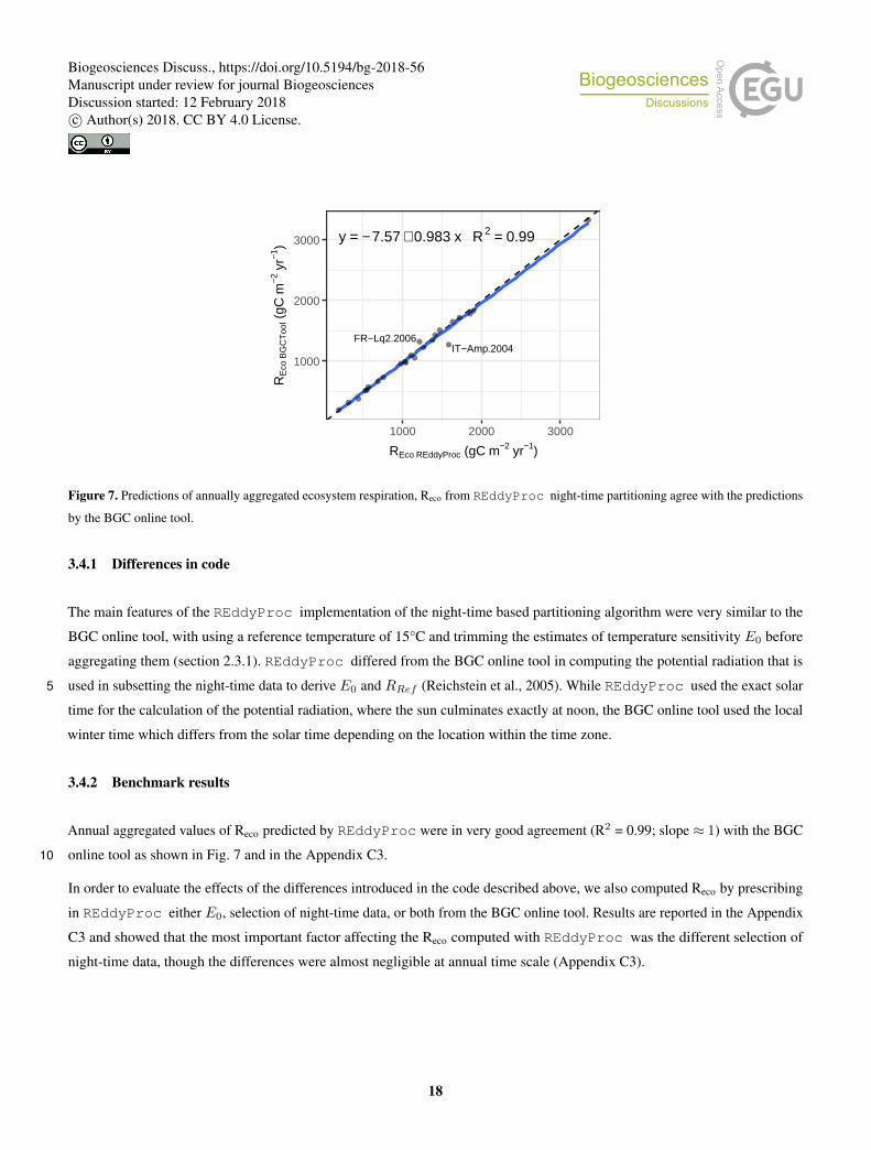
Figure 7. Predictions of annually aggregated ecosystem respiration, Reco from REddyProc night-time partitioning agree with the predictions

by the BGC online tool.

3.4.1 Differences in code

The main features of the REddyProc implementation of the night-time based partitioning algorithm were very similar to the

BGC online tool, with using a reference temperature of 15°C and trimming the estimates of temperature sensitivity E0 before

aggregating them (section 2.3.1). REddyProc differed from the BGC online tool in computing the potential radiation that is

used in subsetting the night-time data to derive E0 and RRef (Reichstein et al., 2005). While REddyProc used the exact solar5

time for the calculation of the potential radiation, where the sun culminates exactly at noon, the BGC online tool used the local

winter time which differs from the solar time depending on the location within the time zone.

3.4.2 Benchmark results

Annual aggregated values of Reco predicted by REddyProc were in very good agreement (R2 = 0.99; slope ≈ 1) with the BGC

online tool as shown in Fig. 7 and in the Appendix C3.10

In order to evaluate the effects of the differences introduced in the code described above, we also computed Reco by prescribing

in REddyProc either E0, selection of night-time data, or both from the BGC online tool. Results are reported in the Appendix

C3 and showed that the most important factor affecting the Reco computed with REddyProc was the different selection of

night-time data, though the differences were almost negligible at annual time scale (Appendix C3).

18


3.4.3 Discussion of nighttime flux-partitioning

The two implementations agree very well for most sites at annual time-scale. Because of no systematic deviations across sites,

the spatial upscaling of fluxes should not be affected by REddyProc implementation. However, for some sites, such as IT-Amp,

the quite large relative errors indicates problems related to selection of night-time data and problems due to a large gaps in a

dataset.5

3.5 Daytime flux-partitioning: Benchmark with BGC online tool

The daytime flux-partitioning was benchmarked with results of the BGC online tool. The online tool used pvWave code

developed by Lasslop et al. (2010) that was used with slight variations also in the processing of the 2015 Fluxnet release

(Pastorello et al., 2017).

3.5.1 Differences in code10

The BGC online tool differed from REddyProc (section 2.3.2) mainly in aspects of separation of nighttime data, estimation of

temperature sensitivity from night-time data, uncertainty estimation, treatment of missing values, and optimization library code.

While for separating nighttime data REddyProc used exact solar time where sun culminates exactly at noon, the BGC online

tool used the local winter time zone time.

For the estimation of temperature sensitivity E0 from night-time data the BGC online tool used a reference temperature of 1515

°C, instead of the median temperature inside the window. Hence, it estimated stronger correlations between parameters for

windows with a different temperature range. Moreover, it omitted smoothing of the estimated E0 across time, often leading to

large fluctuations of the E0 estimates across few days (Fig. C6), larger estimates of its uncertainty, and differences in subsequent

estimation of LRC parameters.

For uncertainty estimation, the BGC online tool relied on the curvature of the LRC fit’s optimum instead of a bootstrap20

procedure. Hence, it could not take into account the uncertainty of E0 estimated from night-time data before the daytime LRC

fit. Moreover, during interpolation of fluxes based on previous and next valid estimates, the distance weights differed. While

REddyProc assigned the estimates to the time of the mean of valid record in a window, the BGC online tool assigned it to the

start of the third day, also if there were only valid data for the first day in the window.

For weighting the records in the LRC fit, the BGC online tool used the raw estimated NEE uncertainty of each record. It did25

not check for high leverage of spurious low NEE uncertainty estimates. Its estimates, therefore, were in some windows very

strongly influenced by a few records, and failed if a NEE uncertainty estimate of zero was provided. Moreover, when there were

missing values or values below zero in provided NEE uncertainty, it set all uncertainty to 1, while REddyProc filled the gaps

by setting the missing uncertainty to the maximum of 20% of respective NEE but at least 0.7 µmolCO2m−2s−1.

19


y = 2.89 + 0.979 x R2 = 0.98

RU−Cok

1000

2000

3000

1000 2000 3000

GPPREddyProc_Default (gC m−2 yr−1)

GP

PB

GC

Tool (

gC m

−2 y

r−1)

Figure 8. Prediction of annually aggregated GPP from REddyProc daytime partitioning agree with the BGC online tool across sites.

Treatment of missing values was not considered by the BGC online tool and assumed to be handled prior to the processing.

Hence, it did not handle missing VPD values and did not re-try the LRC fit without the VPD-effect in order to use also records

with missing VPD. Moreover, as described above, when there were missing values of NEE uncertainty, weighting records in the

LRC fit was omitted.

For compatibility with the BGC online tool, the above code-differences can be disabled in REddyProc. But differences in5

optimization library code and specifically the conditions of non-convergence on scattered data could not be eliminated, which

led to differences in results as shown in the following section.

3.5.2 Benchmark results for day-time partitioning

Annually GPP predictions of both implementations showed no significant bias across the test sites (Fig. 8), although, there

was some scatter for the individual predictions. A similar scatter was observed when comparing the predictions of the default10

REddyProc options to the predictions with compatibility options. Most of the scatter was caused by skipping the test on high

influence of NEE records with small NEE uncertainty (Appendix Fig. C7).

The largest differences in aggregated fluxes between implementations were due to the extrapolation of fitted parameters to

periods where no parameter fits were obtained. In many of those cases, there were fits at the boundaries of the difficult periods,

whose validity was questionable. Whether those fits passed the quality check or not had a large influence on the extrapolation and15

hence on the aggregated values. For example, at RU-Cok parameter estimates for valid periods agreed between implementations.

However, no valid parameters could be obtained for winter months. While REddyProc reported missing values, the BGC

online tool reported GPP values based on summer parameterizations also for periods further away from summer.

20


Uncertainty estimates of gross fluxes were larger with REddyProc due to accounting for uncertainty in temperature sensitivity

estimate from night-time data (Fig. C5).

3.5.3 Discussion of daytime flux-partitioning

Agreement between aggregated fluxes predicted by the daytime method and absence of bias for the test sites (Fig. 8) suggest

that the methods can be used interchangeably for upscaling, although differences in results of influential sites can potentially5

propagate to differences in upscaled estimates. REddyProc provides a quality flag for the results of the day-time partitioning,

that allows excluding less reliable data in upscaling studies. For the results associated with good quality flags, we set stronger

trust in the REddyProc-based estimates.

The daytime flux-partitioning is quite sensitive to the details of LRC fit. Small changes in treatment of extreme or missing NEE

uncertainty estimates or changes in pre-processing and treatment of missing values cause different estimates of LRC parameters10

and propagate to predicted fluxes of GPP and Reco. Although, we put much effort in trying to reproduce the BGC online tool

results, we were not able to eliminate all differences, especially in the subtle details in the parameter optimization library codes.

The differences in predicted half-hourly fluxes, however, average out across sites and across time (Fig. C8 bottom) making this

issue less severe at larger scales.

The estimated uncertainties are even more sensitive. Both implementations occasionally produce unreasonably high outliers that15

affect the aggregated values. REddyProc, in general, estimates higher uncertainties of predicted fluxes, because it accounts for

uncertainty in temperature sensitivity. Note, that the uncertainty introduced to annually aggregated fluxes due to flux-partitioning

is smaller than uncertainty due to uncertain uStar threshold estimate. Hence, differences or difficulties in uncertainty estimation

caused by flux-partitioning do affect conclusions of the overall uncertainty estimates to a lesser extent.

4 Conclusions20

The REddyProc software provides a set of tools for the CO2-focussed post-processing of eddy covariance flux data including

uStar-filtering, gap-filling and flux-partitioning. The freely available R-package allows flexible integration into extended

workflows and automated routines for the propagation of the uncertainty from the uStar-filtering to the gap-filled NEE and

partitioned GPP and Reco.

The compatibility of the implemented methods to the available standard tools provides continuity of the data analysis, when25

adopting REddyProc for processing EC-data. REddyProc can closely reproduce results of the widely used BGC online tool.

A number of enhancements provide more flexibility to the user in the processing of their data. For instance, the new processing

allows to treat multi-year data without breaks at annual boundaries that can significantly affect sites in the southern hemisphere

or sites characterized by vegetation activity in winter. Another new feature of REddyProc is the flexibility to define different

21


seasons for the application of the uStar-filtering and gap-filling routines, which is important for sites with discontinuous surface

cover associated with snow melt, dry seasons, or harvest.

Sensitivity of the results to subtle details of the implementation, however, call for caution when interpreting results. This is

especially true for uStar threshold estimation and the daytime-based flux-partitioning, and especially for data with long gaps.

Continued integration of new methodological developments into the package will support research using EC data. We strive to5

provide new developments in a basic and extensible manner, while paying attention to compatibility with results of reference

implementations.

In summary, research using (half-)hourly eddy covariance data can benefit from building blocks for standardized and extensible

post-processing provided by REddyProc.

Appendix A: The REddyProc package10

The processing tool is freely available in two options: a) online as a web-service2 with a smaller range of user option, and b) as a

package of the open-source R environment with a larger set of user options and with each of the steps and methods available

independently.

The REddyProc package can be installed by typing at the R-terminal:

install.packages("REddyProc")

library(REddyProc)

?REddyProc

15

A1 General design

There are some general principles and choices in the design of REddyProc that explain some trade-offs.

Preventing accidental errors is one goal of the package. Therefore, there is extensive checking on formatting and data

availability when importing the data and also throughout post-processing steps. Especially, the high-level routines will issue

warnings or stop post-processing if they detect inconsistencies or lack of sufficient data, or changes in specification of critical20

standard parameters. These checks reinforce a sound standard post-processing also for non-expert users. On the other hand,

these checks will render the standard routines not usable for datasets where not enough data are available. It is still possible

to use REddyProc with sparse data for some purposes by using lower-level routines. But this requires experience in both,

post-processing and R programming.

Smooth inter-annual processing is the next goal. The data is not partitioned into annual chunks for post-processing to avoid25

artificial discontinuities between years. The user can still specify different periods or seasons, e.g. when meteorological

2 www.bgc-jena.mpg.de/bgi/index.php/Services/REddyProcWeb

22


conditions change after harvest, but the boundaries do not need to align with years. REddyProc therefore works with the entire

dataset in memory. Potentially this can lead to longer post-processing times when working with many years of EC data but still

can be handled on a usual notebook.

Memory efficient processing required some extended R programming. Specifically we used R5 classes3 to avoid frequently

copying the entire dataset in memory. Users should be aware that calling functions on the sEddyProc class not only provides a5

return value but also changes the data of the R5 class (Chapter ’OO field guide’ in Wickham, 2014). Users who want to integrate

the post-processing in their own codes are encouraged to learn about R5 classes, however, it is not a prerequisite.

Continuity with other tools ensures that switching to REddyProc does not introduce discontinuities with results obtained

from other tools. Specifically, we reproduced the uStar threshold estimation of the C implementation by Dario Papale, and the

gap-filling, night-time flux partitioning, and day-time flux-partitioning from the BGC online tool (Reichstein et al., 2005). In10

some details, the standard parameterization differs from the old tool, e.g. using seasons that span across calendar years in uStar

threshold estimation, but it is usually possible to set compatible parameters with REddyProc.

Appendix B: Example application

This section reports an example R session using REddyProc. Code is shown in a shaded area and corresponding output with

monospace font.15

B1 Importing the half-hourly data

The workflow starts with importing the half-hourly data. The example reads a text file with data of the year 1998 from the

Tharandt site and converts the separate decimal columns year, day, and hour to a POSIX timestamp column. Next, it initializes

the sEddyProc class.

#+++ load libraries used in this vignette

library(REddyProc)

library(dplyr)

#+++ Load data with 1 header and 1 unit row from (tab-delimited) text file

fileName <- getExamplePath('Example_DETha98.txt', isTryDownload = TRUE)

EddyData.F <- if (length(fileName)) fLoadTXTIntoDataframe(fileName) else

# or use example dataset in RData format provided with REddyProc

Example_DETha98

#+++ Add time stamp in POSIX time format

EddyDataWithPosix.F <- fConvertTimeToPosix(EddyData.F, 'YDH',Year.s = 'Year'

3 www.rdocumentation.org/packages/methods/versions/3.4.3/topics/ReferenceClasses

23


,Day.s = 'DoY',Hour.s = 'Hour')

#+++ Initalize R5 reference class sEddyProc for post-processing of eddy data

#+++ with the variables needed for post-processing later

EddyProc.C <- sEddyProc$new('DE-Tha', EddyDataWithPosix.F,

c('NEE','Rg','Tair','VPD', 'Ustar'))

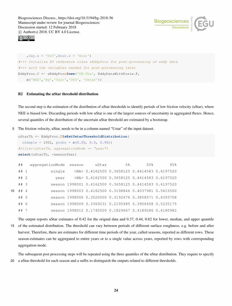
B2 Estimating the uStar threshold distribution

The second step is the estimation of the distribution of uStar thresholds to identify periods of low friction velocity (uStar), where

NEE is biased low. Discarding periods with low uStar is one of the largest sources of uncertainty in aggregated fluxes. Hence,

several quantiles of the distribution of the uncertain uStar threshold are estimated by a bootstrap.

The friction velocity, uStar, needs to be in a column named “Ustar” of the input dataset.5

uStarTh <- EddyProc.C$sEstUstarThresholdDistribution(

nSample = 100L, probs = c(0.05, 0.5, 0.95))

#filter(uStarTh, aggregationMode == "year")

select(uStarTh, -seasonYear)

## aggregationMode season uStar 5% 50% 95%

## 1 single <NA> 0.4162500 0.3658125 0.4414583 0.6197520

## 2 year <NA> 0.4162500 0.3658125 0.4414583 0.6197520

## 3 season 1998001 0.4162500 0.3658125 0.4414583 0.6197520

## 4 season 1998003 0.4162500 0.3198846 0.4037981 0.561550010

## 5 season 1998006 0.3520000 0.3192476 0.3858571 0.4393708

## 6 season 1998009 0.3369231 0.2195485 0.3906458 0.5235175

## 7 season 1998012 0.1740000 0.1829667 0.4189286 0.6180982

The output reports uStar estimates of 0.42 for the orignal data and 0.37, 0.44, 0.62 for lower, median, and upper quantile

of the estimated distribution. The threshold can vary between periods of different surface roughness, e.g. before and after15

harvest. Therefore, there are estimates for different time periods of the year, called seasons, reported as different rows. These

season-estimates can be aggregated to entire years or to a single value across years, reported by rows with corresponding

aggregation mode.

The subsequent post processing steps will be repeated using the three quantiles of the uStar distribution. They require to specify

a uStar-threshold for each season and a suffix to distinguish the outputs related to different thresholds.20

24


For this example of an evergreen forest site, the same annually aggregated uStar threshold estimate will be chosen for each

of the seasons within a year. In order to distinguish the automatically generated columns, the column names of the estimation

results are written to variable uStarSuffixes.

uStarThAnnual <- usGetAnnualSeasonUStarMap(uStarTh)[-2]

uStarSuffixes <- colnames(uStarThAnnual)[-1]

print(uStarThAnnual)

## season U05 U50 U95

## 1 1998001 0.3658125 0.4414583 0.6197525

## 2 1998003 0.3658125 0.4414583 0.619752

## 3 1998006 0.3658125 0.4414583 0.619752

## 4 1998009 0.3658125 0.4414583 0.619752

## 5 1998012 0.3658125 0.4414583 0.619752

B3 Gap-filling10

The second post-processing step is filling the gaps using information of the valid data. In this case, the same annual uStar

threshold estimate is used for each season, as described above, and the uncertainty will be computed also for valid records

(FillAll).

EddyProc.C$sMDSGapFillAfterUStarDistr('NEE',

UstarThres.df = uStarThAnnual,

UstarSuffix.V.s = uStarSuffixes,

FillAll = TRUE

)

The screen output (not shown here) already shows that the uStar-filtering and gap-filling was repeated for each given estimate of

the uStar threshold , i.e. column in uStarThAnnual, with marking 22% to 38% of the data as gap.15

For each of the different uStar threshold estimates, a separate set of output columns of filled NEE and its uncertainty is generated,

distinguished by the suffixes given with uStarSuffixes. Suffix “_f" denotes the filled value and “_fsd" the estimated

standard devation of its uncertainty.

grep("NEE_.*_f$",names(EddyProc.C$sExportResults()), value = TRUE)

grep("NEE_.*_fsd$",names(EddyProc.C$sExportResults()), value = TRUE)

## [1] "NEE_U05_f" "NEE_U50_f" "NEE_U95_f"

## [1] "NEE_U05_fsd" "NEE_U50_fsd" "NEE_U95_fsd"20

25


B4 Partitioning net flux into GPP and Reco

The third post-processing step is partitioning the net flux (NEE) into its gross components GPP and Reco. The partitioning

algorithm needs a precise criteria between night-time and day-time. Therefore, the specification of geographical coordinates and

time zone need to be provided to allow computing exact solar time of sunrise and sunset. Further, the missing values in the used

meteorological data need to be filled.5

EddyProc.C$sSetLocationInfo(Lat_deg.n = 51.0, Long_deg.n = 13.6, TimeZone_h.n = 1)

EddyProc.C$sMDSGapFill('Tair', FillAll.b = FALSE)

EddyProc.C$sMDSGapFill('VPD', FillAll.b = FALSE)

Now we are ready to invoke the partitioning, here by the night-time approach, for each of the several filled NEE columns.

#variable uStarSuffixes was defined above at the end of uStar threshold estimation

resPart <- lapply(uStarSuffixes, function(suffix){

EddyProc.C$sMRFluxPartition(Suffix.s = suffix)

})

The results are stored in columns Reco and GPP_f modified by the respective uStar threshold suffix.

grep("GPP.*_f$|Reco",names(EddyProc.C$sExportResults()), value = TRUE)

## [1] "Reco_U05" "GPP_U05_f" "Reco_U50" "GPP_U50_f" "Reco_U95" "GPP_U95_f"

The visualizations of the results by a fingerprint plot gives a compact overview.

EddyProc.C$sPlotFingerprintY('GPP_U50_f', Year.i = 1998)

0 4 8 12 16 20 24

Jan

May

Oct

10

B5 Estimating the uncertainty of aggregated results

First, the mean of the GPP across all the year is computed for each uStar-scenario and converted from µmol CO2 m−2s−1 to

gC m−2yr−1.

26


FilledEddyData.F <- EddyProc.C$sExportResults()

#suffix <- uStarSuffixes[2]

GPPAggCO2 <- sapply( uStarSuffixes, function(suffix) {

GPPHalfHour <- FilledEddyData.F[[paste0("GPP_",suffix,"_f")]]

mean(GPPHalfHour, na.rm = TRUE)

})

molarMass <- 12.011

GPPAgg <- GPPAggCO2 * 1e-6 * molarMass * 3600*24*365.25

print(GPPAgg)

## U05 U50 U95

## 1894.097 1956.090 1985.817

The difference between those aggregated values is a first estimate of uncertainty range in GPP due to uncertainty of the uStar

threshold.

(max(GPPAgg) - min(GPPAgg)) / median(GPPAgg)

In this run of the example a relative error of about 4.7% is inferred.5

For a better but more time consuming uncertainty estimate, specify a larger sample of uStar threshold values, for each repeat the

post-processing, and compute statistics from the larger sample of resulting GPP columns. This can be achieved by specifying a

larger sequence of quantiles when calling sEstUstarThresholdDistribution.

sEstUstarThresholdDistribution(

nSample = 200, probs = seq(0.025,0.975,length.out = 39) )

B6 Storing the results in a csv-file

The results still reside inside the sEddyProc class. To export them to an R Data.frame, the newly generated columns need to10

be appended to the columns with the original input data. Then this data.frame is written to a text file in a temporary directory.

FilledEddyData.F <- EddyProc.C$sExportResults()

CombinedData.F <- cbind(EddyData.F, FilledEddyData.F)

fWriteDataframeToFile(CombinedData.F, 'DE-Tha-Results.txt', Dir.s = tempdir())

B7 Specifying seasons where uStar thresholds differs

With changing surface roughness, e.g. on harvest or leaf-fall, also the uStar-NEE relationship can change. Therefore the

uStar threshold needs to be re-estimated at different times of the year, called seasons. The default uses continuous sea-

27


sons, for details see section 3.2.1. In order to yield results corresponding to DP06, the user can specify seasonFactor.v =

usCreateSeasonFactorMonthWithinYear( EddyData.C$sDATA$sDateTime, startMonth= c(3,6,9,12)) as an argument to

routine sEstUstarThreshold. By default the annual aggregate of the season thresholds, i.e. maximum across seasons, is used to

identify unfavorable conditions. The seasonal estimates can also be used instead.

Moreover, the users can specify also other user-defined seasons, e.g. when harvest dates are known (see package5

vignette DEGebExample). They can create a grouping by specifying exact starting days of the periods by function

usCreateSeasonFactorYdayYear, or they can provide a column with the data that indicates e.g. the same group for two wet

seasons. Each season is associated to the year corresponding to the center day between first and last day of the season.

With all methods, there is a required minimum number of 160 records within a season. If there are too few records, the data of

the seasons within one year are combined and the uStar threshold for this seasons is set to the estimate obtained for the data of10

the entire year.

Appendix C: Additional benchmark statistics

This section provides figures, in addition to the main figures presented in the benchmark section (3), that require the reader

being comfortable with histograms and probability distribution functions.

The histograms display how often a certain value occurs across all the site-months. A centering of a difference away from zero15

or for a ratio away from one denotes a bias.

C1 uStar Threshold estimation

There was a bias in uStar estimation (Fig. C1). However, the bias and the differences were only a small fraction of the uncertainty

of the estimate itself. Moreover, the bias did not propagate through estimated NEE based on different uStar values (Fig. C2).

There was a significant difference in the estimate of uncertainty of the uStar thresholds (Fig. C3). REddyProc only estimated20

half of the uncertainty due to acknowledging the seasons of similar conditions also during bootstrap. This lower uncertainty

propagated to the uncertainty estimates of NEE (Fig. C4)

C2 Gap-filling

The evaluation of annual aggregated NEE data obtained with REddyProc and the BGC online tool showed good agreement

across sites.25

Note, that the aggregated NEE data contained both, measured and gap-filled data for the purpose of evaluating the impact of

the processing on the aggregated NEE. The determination coefficient (R2) showed a very good agreement between the two

28


0

2

4

6

−1.0 −0.5 0.0 0.5 1.0

relative deviation in uStar threshold

coun

t of s

ite_y

ears

Figure C1. Histogram of differences between uStar threshold estimates of different methods (DP06 - REddyProc) normalized by the

uncertainty range (90% quantile - 10% quantile estimated by DP06). Absolute values are smaller than one meaning that the difference between

the methods is smaller than range of estimates by the DP06 method only. The clustering of values on the positive side suggests a bias towards

larger values with DP06.

0

1

2

3

4

5

−1 0 1

relative NEE deviation

coun

t of s

ite_y

ears

Figure C2. Histogram of differences between annual NEE based on uStar estimates of different methods (Papale - REddyProc) normalized

by the uncertainty range of NEE due to uStar (NEE based on 90% uStar quantile - NEE based on 10% uStar quantile estimated by DP06).

Absolute values are mostly smaller than one, meaning that the difference in annual NEE between methods is smaller than the uncertainty due

to uncertainty of uStar threshold from DP06 only.

methods both at annual and monthly time scale (Table C1). The relative mean absolute error (RMAE) is low: about -3 % for

annual aggregation and -0.47 % for monthly aggregation. Both Modeling Efficiency (EF) and Mean Bias Error (MBE) showed a

very low bias between the two products for both monthly and annual aggregations (Table C1).

29


0

1

2

3

4

5

0.0 0.5 1.0 1.5

relative uStar uncertainty range

coun

t of s

ite_y

ears

Figure C3. Histogram of ratio (REddyProc / DP06) of uncertainty ranges of uStar (90% quantile - 10% quantile). The clustering around

0.5 shows that the estimated uncertainty with REddyProc is only about half the uncertainty estimated by DP06.

0

1

2

3

4

0.0 0.5 1.0 1.5

relative NEE uncertainty range

coun

t of s

ite_y

ears

Figure C4. Histogram of ratio (REddyProc / DP06) of uncertainty ranges of annual NEE (NEE based on 90% quantile of uStar threshold -

NEE based on 10% qunatile of uStar threshold). The clustering below a value of one indicates that the lower uncertainty in uStar threshold

with REddyProc also propagates to lower uncertainty in annual NEE.

30


Table C1. Gap-filling evaluation statistics of yearly (Fig. 6) and monthly cumulated and gap-filled NEE data obtained with REddyProc and

the BGC online tool. Statistic abbreviations are explained in section C2.

Yearly Monthly

N 25 281

pearson 0.99 1.00

MBE -0.02 0.00

RMBE 2.8% -0.08%

MAE 0.02 0.00

RMAE -3.0% -0.5%

RMSE 0.09 0.01

R2 0.98 1.00

EF 0.98 1.00

31


C3 Night-time partitioning

The results show good agreement between Reco estimated using REddyProc and the BGC online tool for R2 and EF (Table

C2). The relative RMSE is 6.56 and 13.45 % for yearly and monthly aggregation, respectively. The high RRMSE is due to

few site years as reported in Table C3, and this is confirmed by the lower RMAE (3.87 % and 6.33 % for yearly and monthly,

respectively), which is less sensitive to outliers.5

The difference in Reco related to the selection of night-time data are not negligible: the differences in RRMSE of 1.03% and

negligible differences in R2. Also, the use of E0 prescribed from the BGC online tool lead to negligible difference in R2

of about 0.02. Therefore, though very small, the selection of night-time data is the most important difference introduced by

REddyProc .

Table C2. Nighttime partitioning evaluation statistics across sites of annually (Fig. 7) and monthly aggregated ecosystem respiration (Reco)

estimated with REddyProc and the BGC online tool.

Yearly Monthly

N 25 297

pearson 0.99 0.99

MBE 25.4 2.15

RMBE 2.2% 2.2%

MAE 44.8 6.17

RMAE 3.8% 6.3%

RMSE 75.6 13.2

RRMSE 6.5% 13.5%

R2 0.99 0.98

EF 0.99 0.97

C4 Day-time partitioning10

The time-variable estimate of temperature sensitivity of ecosystem respiration with day-time partitioning is a significant source

of uncertainty for gross fluxes GPP and Reco. REddyProc accounts for this previously unaccounted uncertainty for estimating

uncertainty of these gross fluxes by a bootstrap (Fig. C5). The estimate of annual uncertainty in Fig. C5 is a low estimate,

because it assumed no correlation between half-hourly errors. An improved quantification of correlations requires the full

variance-covariance matrix of the LRC parameter fits (Lasslop et al., 2010; Menzer et al., 2013), which were not available for15

the BGC online tool.

The introduced uncertainty is reduced by smoothing the E0 estimates across several successive windows (Fig. C5 top) before

estimating parameters of the LRC. This smoothing has also an effect on predicted half-hourly gross fluxes (Fig. C5 bottom).

32


RMBE RMAE RRMSE R2 EF

CA-NS7 15.12 16.29 32.64 0.96 0.86

CA-TP3 -1.99 25.10 38.59 0.87 0.82

DE-Hai 6.00 6.48 10.40 0.99 0.96

DE-Tha 2.83 3.52 6.19 0.99 0.99

DK-Sor 3.50 4.45 7.34 1.00 0.99

ES-ES1 1.68 3.34 4.59 0.93 0.92

ES-VDA 3.96 9.98 15.93 0.95 0.93

FI-Hyy 2.72 3.05 4.47 1.00 1.00

FI-Kaa -4.52 5.51 9.07 0.99 0.99

FR-Gri 3.96 4.14 6.35 1.00 0.99

FR-Hes 4.11 5.06 9.06 0.99 0.99

FR-Lq1 -2.89 5.76 7.24 0.99 0.99

FR-Lq2 -8.27 9.49 11.49 0.99 0.97

FR-Pue 0.65 1.27 1.55 1.00 1.00

IE-Dri -0.03 2.41 3.24 1.00 1.00

IL-Yat 1.66 2.89 3.72 0.99 0.99

IT-Amp 24.34 29.38 45.33 0.91 0.48

IT-MBo 2.03 3.00 4.49 1.00 1.00

IT-SRo -1.46 1.86 2.10 1.00 0.99

PT-Esp 9.06 12.08 19.94 0.62 0.45

RU-Cok -0.76 28.54 38.98 0.27 -0.07

SE-Nor -1.05 2.09 3.62 1.00 1.00

US-Ton 2.93 7.45 11.82 0.93 0.92

VU-Coc 0.73 2.64 3.83 0.93 0.93Table C3. Nighttime partitioning evaluation statistics at sites level of the of ecosystem respiration (Reco) estimated with REddyProc and the

BGC online tool.

Results of daytime partitioning are sensitive to subtle details of the procedure. Hence, there is quite much scatter introduced by

the differences of processing REddyProc with default options or with options that maximize compatibility with the BGC

online tool (Fig. C7 top). One such a subtle options is to decrease or to not account for the unreasonably high leverage of some

observations during the fit to the light-response curve by some records having a very small estimate of its uncertainty (Fig. C7

bottom). Due to the sensitivities of the day-time partitioning, there are still differences between REddyProc with compatibility5

options and the BGC online tool (Fig. C8).

33


0.000

0.005

0.010

0 200 400 600

sdGPP (gC m−2 yr−1)

dens

ity

BGCTool

REddyProc_Default

Figure C5. Density plot of estimated standard deviation of uncertainty of the annually aggregated GPP across sites due to uncertainty in

parameters estimation during day-time based flux partitioning. Higher estimates with REddyProc are caused by taking into account the

uncertainty in temperature sensitivity, E0.

100

200

300

Mrz 01 Mrz 15 Apr 01 Apr 15 Mai 01

E0

(K)

0

5

10

15

20

Apr 05 Apr 12 Apr 19

GP

P (

µ m

ol C

O2

m−2

s−1

)

Default omitSmoothTempSens

Figure C6. Effects of smoothing (top) successive estimates of temperature sensitivity, E0, on predicted GPP (bottom) for site PT-Esp.

Acknowledgements. This work used eddy covariance data acquired and shared by the FLUXNET community, including these networks:

AmeriFlux, AfriFlux, AsiaFlux, CarboAfrica, CarboEuropeIP, CarboItaly, CarboMont, ChinaFlux, Fluxnet-Canada, GreenGrass, ICOS,

KoFlux, LBA, NECC, OzFlux-TERN, TCOS-Siberia and USCCC. The ERA-Interim reanalysis data are provided by ECMWF and processed

by LSCE. The FLUXNET eddy covariance data processing and harmonization was carried out by the European Fluxes Database Cluster,

AmeriFlux Management Project, and Fluxdata project of FLUXNET, with the support of CDIAC and ICOS Ecosystem Thematic Center, and5

the OzFlux, ChinaFlux and AsiaFlux offices.

34


y = 2.2 + 0.992 x R2 = 1

0

2000

4000

0 2000 4000


GP

PR

Edd

yPro

c_La

sslo

p10

(gC

m−2

yr−1

)

y = 6.35 + 0.991 x R2 = 1

0

2000

4000

0 2000 4000


GP

Pom

it_B

ound

NE

EU

ncer

tain

ty (

gC m

−2 y

r−1)

Figure C7. Sensitivity of estimated monthly GPP fluxes to specific processing details results in scatter between GPP predictions based on

different REddyProc options. Most of the differences between default options and compatibility options (top) are caused by differences in

weighting different records during the fit (bottom.)

0

30

60

90

−500 0 500 1000

GPPBGCTool − GPPREddyProc_Lasslop10 (gC m−2 yr−1)

coun

t

Figure C8. Histogram of difference between monthly GPP predictions of REddyProc with Lasslop10 compatibility options and the BGC

online tool.

The authors acknowledge Dario Papale, Gilberto Pastorello and Trevor F Keenan for the discussions on the benchmarking of REddyProc and

PvWave code. M. M. and M. R. acknowledge the Alexander Von Humbold foundation that funded part of this research activity with the Max

Planck Research Preis to Markus Reichstein. M. M. acknowledge the MSCA-ITN project TRUSTEE.

35


L.Š. was supported by the Ministry of Education, Youth and Sports of the Czech Republic within the CzeCOS program, grant number

LM2015061, and within the National Sustainability Program I (NPU I), grant number LO1415.

36


References

Aubinet, M., Grelle, A., Ibrom, A., Rannik, U., Moncrieff, J., Foken, T., Kowalski, A. S., Martin, P. H., Berbigier, P., Bernhofer, C., Clement,

R., Elbers, J., Granier, A., Grünwald, T., Morgenstern, K., Pilegaard, K., Rebmann, C., Snijders, W., Valentini, R., and Vesala, T.: Estimates

of the annual net carbon and water exchange of European forests: The EUROFLUX methodology, Advances in Ecological Research, 30,

114–177, 2000.5

Aubinet, M., Vesala, T., and Papale, D., eds.: Eddy Covariance, Springer Netherlands, https://doi.org/10.1007/978-94-007-2351-1, 2012.

Baldocchi, D., Chu, H., and Reichstein, M.: Inter-annual variability of net and gross ecosystem carbon fluxes: A review, Agricultural and

Forest Meteorology, https://doi.org/10.1016/j.agrformet.2017.05.015, 2017.

Barr, A., Richardson, A., Hollinger, D., Papale, D., Arain, M., Black, T., Bohrer, G., Dragoni, D., Fischer, M., Gu, L., et al.: Use of change-

point detection for friction–velocity threshold evaluation in eddy-covariance studies, Agricultural and forest meteorology, 171, 31–45,10

https://doi.org/10.1016/j.agrformet.2012.11.023, 2013.

Chapin, F. S., Woodwell, G. M., Randerson, J. T., Rastetter, E. B., Lovett, G. M., Baldocchi, D. D., Clark, D. A., Harmon, M. E., Schimel,

D. S., Valentini, R., Wirth, C., Aber, J. D., Cole, J. J., Goulden, M. L., Harden, J. W., Heimann, M., Howarth, R. W., Matson, P. A., McGuire,

A. D., Melillo, J. M., Mooney, H. A., Neff, J. C., Houghton, R. A., Pace, M. L., Ryan, M. G., Running, S. W., Sala, O. E., Schlesinger,

W. H., and Schulze, E. D.: Reconciling carbon-cycle concepts, terminology, and methods, Ecosystems, 9, 1041–1050, 2006.15

Davison, A. and Hinkley, D.: Bootstrap methods and their application, Cambridge University Press, Cambridge, 1997.

Desai, A. R., Richardson, A. D., Moffat, A. M., Kattge, J., Hollinger, D. Y., Barr, A., Falge, E., Noormets, A., Papale, D., Reichstein, M., and

Stauch, V. J.: Cross-site evaluation of eddy covariance GPP and RE decomposition techniques, Agricultural and Forest Meteorology, 148,

821 – 838, https://doi.org/https://doi.org/10.1016/j.agrformet.2007.11.012, 2008.

Efron, B. and Tibshirani, R.: Bootstrap methods for standard errors, confidence intervals, and other measures of statistical accuracy, Statistical20

science, pp. 54–75, 1986.

Falge, E., Baldocchi, D., Olson, R. J., Anthoni, P., Aubinet, M., Bernhofer, C., Burba, G., Ceulemans, R., Clement, R., Dolman, H., Granier,

A., Gross, P., Grünwald, T., Hollinger, D., Jensen, N. O., Katul, G., Keronen, P., Kowalski, A., Ta Lai, C., Law, B. E., Meyers, T., Moncrieff,

J., Moors, E., Munger, J. W., Pilegaard, K., Rannik, U., Rebmann, C., Suyker, A., Tenhunen, J., Tu, K., Verma, S., Vesala, T., Wilson, K.,

and Wofsy, S.: Gap filling strategies for defensible annual sums of net ecosystem exchange, Agric. For. Meteorol., 107/1, 29–43, 2001.25

Foken, T. and Wichura, B.: Tools for quality assessment of surface-based flux measurements, Agricultural and forest meteorology, 78, 83–105,

https://doi.org/10.1016/0168-1923(95)02248-1, 1996.

Foken, T., Göockede, M., Mauder, M., Mahrt, L., Amiro, B., and Munger, W.: Post-field data quality control, in: Handbook of micrometeorology,

pp. 181–208, Springer, 2004.

Foken, T., Leuning, R., Oncley, S. R., Mauder, M., and Aubinet, M.: Corrections and Data Quality Control, pp. 85–131, Springer Netherlands,30

Dordrecht, https://doi.org/10.1007/978-94-007-2351-1_4, 2012.

Gilmanov, T. G., Johnson, D. A., and Saliendra, N. Z.: Growing season CO2 fluxes in a sagebrush-steppe ecosystem in Idaho: bowen

ratio/energy balance measurements and modeling, Basic and Applied Ecology, 4, 167 – 183, https://doi.org/http://dx.doi.org/10.1078/1439-

1791-00144, 2003.

Gorsel, E. V., Leuning, R., Cleugh, H. A., Keith, H., and Suni, T.: Nocturnal carbon efflux: reconciliation of eddy covariance and chamber35

measurements using an alternative to the u.-threshold filtering technique, Tellus B: Chemical and Physical Meteorology, 59, 397–403, 2007.

37


Göckede, M., Rebmann, C., and Foken, T.: A combination of quality assessment tools for eddy covariance measurements

with footprint modelling for the characterisation of complex sites, Agricultural and Forest Meteorology, 127, 175–188,


Jung, M., Reichstein, M., Margolis, H. A., Cescatti, A., Richardson, A. D., Arain, M. A., Arneth, A., Bernhofer, C., Bonal, D., Chen, J.,

Gianelle, D., Gobron, N., Kiely, G., Kutsch, W., Lasslop, G., Law, B. E., Lindroth, A., Merbold, L., Montagnani, L., Moors, E. J., Papale,5

D., Sottocornola, M., Vaccari, F., and Williams, C.: Global patterns of land-atmosphere fluxes of carbon dioxide, latent heat, and sensible

heat derived from eddy covariance, satellite, and meteorological observations, Journal of Geophysical Research: Biogeosciences, 116,

n/a–n/a, 2011.

Körner, C.: Leaf Diffusive Conductances in the Major Vegetation Types of the Globe, pp. 463–490, Springer Berlin Heidelberg, Berlin,

Heidelberg, https://doi.org/10.1007/978-3-642-79354-7_22, 1995.10

Lasslop, G., Reichstein, M., Papale, D., Richardson, A., Arneth, A., Barr, A., Stoy, P., and Wohlfahrt, G.: Separation of net ecosystem exchange

into assimilation and respiration using a light response curve approach: critical issues and global evaluation, Global Change Biology, 16,

187–208, https://doi.org/10.1111/j.1365-2486.2009.02041.x, 2010.

Lloyd, J. and Taylor, J.: On the temperature dependence of soil respiration, Functional ecology, 8, 315–323, 1994.

Massman, W. J. and Lee, X.: Eddy covariance flux corrections and uncertainties in long-term studies of carbon and energy exchanges,15

Agricultural and Forest Meteorology, 113, 121–144, 2002.

Menzer, O., Moffat, A. M., Meiring, W., Lasslop, G., Schukat-Talamazzini, E. G., and Reichstein, M.: Random errors in

carbon and water vapor fluxes assessed with Gaussian Processes, Agricultural and Forest Meteorology, 178-179, 161–172,


Moffat, A. M.: A new methodology to interpret high resolution measurements of net carbon fluxes between terrestrial ecosystems and the20

atmosphere, Ph.D. thesis, Friedrich-Schiller-Universität Jena, 2012.

Moffat, A. M., Papale, D., Reichstein, M., Hollinger, D. Y., Richardson, A. D., Barr, A. G., Beckstein, C., Braswell, B. H., Churkina, G.,

Desai, A. R., et al.: Comprehensive comparison of gap-filling techniques for eddy covariance net carbon fluxes, Agricultural and Forest

Meteorology, 147, 209–232, https://doi.org/10.1016/j.agrformet.2007.08.011, 2007.

Muggeo, V.: Segmented: An R package to fit regression models with broken-line relationships, R News, 8 (1), 20: 25, 2008.25

Muggeo, V. M.: Estimating regression models with unknown break-points, Statistics in medicine, 22, 3055–3071, 2003.

Papale, D., Reichstein, M., Aubinet, M., Canfora, E., Bernhofer, C., Kutsch, W., Longdoz, B., Rambal, S., Valentini, R., Vesala, T., and et al.:

Towards a standardized processing of Net Ecosystem Exchange measured with eddy covariance technique: algorithms and uncertainty

estimation, Biogeosciences, 3, 571 – 583, https://doi.org/10.5194/bg-3-571-2006, 2006.

Pastorello, G., Papale, D., Chu, H., Trotta, C., Agarwal, D., Canfora, E., Baldocchi, D., and Torn, M.: The FLUXNET2015 dataset: The30

longest record of global carbon, water, and energy fluxes is updated, Eos Trans. AGU, https://doi.org/10.1029/2017EO071597, 2017.

Rasmussen, C. E. and Williams, C. K. I.: Gaussian Processes for Machine Learning, The MIT Press, 2006.

Rebmann, C., Kolle, O., Heinesch, B., Queck, R., Ibrom, A., and Aubinet, M.: Data Acquisition and Flux Calculations, pp. 59–83, Springer

Netherlands, Dordrecht, https://doi.org/10.1007/978-94-007-2351-1_3, 2012.

Reichstein, M., Falge, E., Baldocchi, D., Papale, D., Aubinet, M., Berbigier, P., Bernhofer, C., Buchmann, N., Gilmanov, T., Granier, A., et al.:35

On the separation of net ecosystem exchange into assimilation and ecosystem respiration: review and improved algorithm, Global Change

Biology, 11, 1424–1439, https://doi.org/10.1111/j.1365-2486.2005.001002.x, 2005a.

38


Reichstein, M., Katterer, T., Andren, O., Ciais, P., Schulze, E. D., Cramer, W., Papale, D., and Valentini, R.: Temperature sensitivity of

decomposition in relation to soil organic matter pools: critique and outlook, Biogeosciences, 2, 317–321, https://doi.org/10.5194/bg-2-317-

2005, 2005b.

Reichstein, M., Subke, J. A., Angeli, A. C., and Tenhunen, J. D.: Does the temperature sensitivity of decomposition of soil organic matter

depend upon water content, soil horizon, or incubation time?, Global Change Biology, 11, 1754–1767, 2005c.5

Reichstein, M., Stoy, P. C., Desai, A. R., Lasslop, G., and Richardson, A. D.: Partitioning of Net Fluxes, pp. 263–289, Springer Netherlands,

Dordrecht, https://doi.org/10.1007/978-94-007-2351-1_9, 2012.

Stoy, P. C., Katul, G. G., Siqueira, M. B., Juang, J.-Y., Novick, K. A., Uebelherr, J. M., and Oren, R.: An evaluation of models for partitioning

eddy covariance-measured net ecosystem exchange into photosynthesis and respiration, Agricultural and Forest Meteorology, 141, 2 – 18,

https://doi.org/10.1016/j.agrformet.2006.09.001, 2006.10

Wehr, R. and Saleska, S.: An improved isotopic method for partitioning net ecosystem–atmosphere CO 2 exchange, Agricultural and Forest

Meteorology, 214, 515–531, 2015.

Wickham, H.: Advanced R, Taylor & Francis Inc, 2014.

39


Documents

Basic and extensible post-processing of eddy covariance ux