BandiT Blackbody Fitting For Temperature …€¦ · k-Space Associates, Inc., 2182 Bishop Circle East, Dexter, MI 48130 USA (734) 426-7977 • [email protected] • CONFIDENTIAL

k-Space Associates, Inc., 2182 Bishop Circle East, Dexter, MI 48130 USA

(734) 426-7977 • [email protected] • www.k-space.com

CONFIDENTIAL — Not To Be Distributed 1 of 15

Blackbody Fitting fBlackbody Fitting fBlackbody Fitting fBlackbody Fitting for Temperature Determinationor Temperature Determinationor Temperature Determinationor Temperature Determination

((((BandiT BandiT BandiT BandiT ver. 2.ver. 2.ver. 2.ver. 2.52525252, released , released , released , released 5555////2222/1/1/1/14444))))

IntroductionIntroductionIntroductionIntroduction

In addition to band edge thermometry, BandiT software has the capability of performing non-linear least squares fitting of a blackbody thermal radiation curve to spectra in real time. This allows a measurement of the temperature which is independent of the band edge method (U.S. Patent 8,282,273, issued Oct. 9, 2012). Spectral radiance is the fundamental measure of the amount of light that can reach a detector from a diffuse source. It is defined as the emitted power per unit area of emitting surface, per unit solid angle, per unit wavelength. Figure 1 is a plot of the spectral radiance of a blackbody for several different temperatures commonly used in semiconductor processing. Note that the peak shifts to shorter wavelengths as the temperature increases.

Figure 1: Spectral Radiance of a Blackbody




This behavior can be expressed mathematically in the form of Wien’s displacement law (Equation 1).

T

bpeak =λ

Equation 1: Wien’s Displacement Law

Here T is the temperature (in Kelvin), and b is a constant which equals

.

≈

2.8978×106 nm-K (see Appendix A). Note that in the temperature range of interest for typical semiconductor processing, the peak lies in the mid-IR portion of the spectrum. Thus, for the most part, BandiT spectral data comes from the short-wavelength exponential tail below the peak. This often poses a challenge, as the signal intensity is relatively weak in this region.

According to Planck’s law, the spectral radiance I (λ, T) of a blackbody at a given temperature is given by Equation 2:

Equation 2: Planck’s Law

In fitting a function of the form described in Equation 2 to spectra there are four adjustable parameters: the material’s emissivity ε, the tooling factor T.F., the temperature T (in Kelvin), and an optional constant background C. The tooling factor incorporates system-dependent geometrical and sensitivity factors, and therefore must be determined empirically. The tooling factor can be determined by calibrating to a blackbody curve at a known temperature (e.g. from a band edge measurement, RHEED transition, or Si/Al eutectic). In this case the temperature is held fixed at the known value, and the tooling factor is allowed to vary to obtain the best fit. Once the tooling factor is known, a blackbody fit can then be performed in real-time during BandiT data acquisition. In this case, the tooling factor is held fixed, and the temperature is allowed to vary to obtain the best fit. This is the so-called “Locked” mode of operation. This approach assumes that the tooling factor and sample emissivity do not change after calibration. Alternatively, in cases where this assumption may not be valid, the “Free Fit” mode of operation can be used. In this mode both the temperature and tooling factor are allowed to vary in order to obtain the best fit. In principle, this approach is insensitive to viewport coatings as the tooling factor can vary over time to accommodate the resulting decrease in signal intensity. The same holds true for the emissivity.

Ce

hcFTTI

Tkhc B+

−=

1

12..),(

5

2

λλελ




Figure 2: Blackbody Flowchart




However, in practice the best results are typically obtained by calibrating at the highest practical temperature and locking the tooling factor. If the calibration temperature is not known via some other means, a free fit can be done to determine it. Then the tooling factor can be determined as described above. This is the so-called “Self-Calibration” method (Figure 2). Whichever mode is chosen, the non-linear least squares fitting routine requires initial guesses for the four adjustable parameters in Equation 2. The routine is sensitive to the accuracy of these values; if they differ too much from the actual values, the fitting routine will fail to converge. In order to minimize this occurrence, “Auto” mode may be selected. In this mode, approximate values of these parameters are automatically calculated and used as the initial guesses.

A simplified version of the Planck expression can be used to obtain these values. This is the so-called “Wien approximation” (Equation 3). This approximation is valid

in the limit that hc / λkT >> 1. This applies when the wavelength is well below the peak of the spectral radiance in Figure 1, which is typically the case at low temperatures (Note that Wien’s displacement law states that the peak occurs at hc /

λkT ≈ 4.965 − see Appendix A.)

( )12..)(

5

2

>>+≅ −TkhcCe

hcFTI B

Tkhc B λλ

ελ λ

Equation 3: Wien Approximation to Planck’s Law

Neglecting the background C, and performing a suitable transformation, this can be

expressed as a linear function of 1/λ (Equation 4).

( ) ( )λ

ελ1

..2lnln 25

Tk

hcFThcI

B

−≅

Equation 4: Linear Transformation of Wien Approximation

Thus a simple linear least-squares fit can be performed to the linearized spectra. The tooling factor can be extracted from the intercept, and the temperature from the slope. These values can then be used as the initial guesses in fitting to the full Planck expression (Equation 2). Note that this works well in many, but not all circumstances. If for some reason the fitting routine fails to converge when using “Auto” mode, then starting guesses will have to be manually entered in the usual fashion. In addition to providing initial guesses for the fit to Equation 2, the linearized spectra provide a better visual representation of any deviations from an ideal blackbody curve across the spectral range. This allows the user to improve the robustness of the fit by excluding portions of the spectrum. This is particularly useful at low




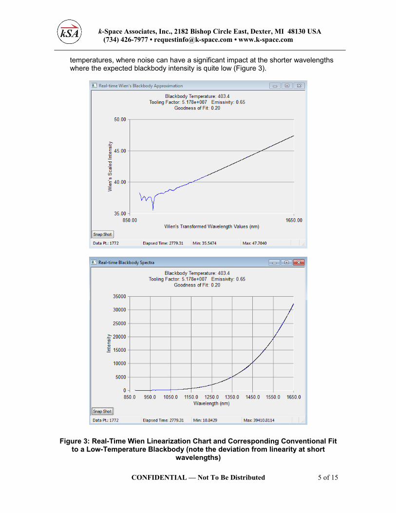
temperatures, where noise can have a significant impact at the shorter wavelengths where the expected blackbody intensity is quite low (Figure 3).

Figure 3: Real-Time Wien Linearization Chart and Corresponding Conventional Fit to a Low-Temperature Blackbody (note the deviation from linearity at short

wavelengths)




ProcedureProcedureProcedureProcedure

Figure 4: Enabling the Spectrometer’s Flat Field Correction

1. Enable Flat Field Correction (FFC):

The spectrometer output has been corrected to yield a flat response as a function of wavelength. This correction is unique to each individual spectrometer. This is a factory calibration and will not need to be adjusted in the field. Before attempting to calibrate blackbody, make sure this correction is enabled. Begin by right-clicking anywhere in the live spectrometer window and selecting Properties (Figure 4 inset). Select the Spectrometer tab, and verify that the Flat Field Correction checkbox is enabled. If not, select the Browse button and select the appropriate FFC file for the spectrometer in question. The default directory is “C:\Program Files\kSA\kSA BandiT\PROGRAM\Spectrometers\SNABnnnn”. Within that folder locate the file “SNABnnnn Blackbody FFC.kdt, where SNABnnnn is the spectrometer’s serial number. When finished, select OK to return to the live spectrometer window. When enabled, FFC on will appear at the bottom right of the live spectrometer window.




2. Calibration: If it is desired to run in Locked mode, the tooling factor must first be calibrated. Begin by selecting Blackbody Calibration from the Acquire menu. Also select the Real-time Blackbody Spectra chart from the View menu (Figure 5). The Blackbody Calibration Acquisition dialog has the following settings:

Figure 5: Blackbody Calibration Acquisition & Real-Time Chart

Select the Spectra source from the pull-down menu. Enter the desired wavelength range over which to perform the blackbody fit.

Entering zeros will cause the software to automatically select the spectrometer’s min and max wavelengths. The values can be locked using the check boxes. Alternatively, if one or both boxes are unchecked, the software will attempt to optimize the goodness of fit by successively reducing the range each time the Calibrate button is pressed.

Enter the Threshold, which specifies the minimum number of counts for performing a blackbody fit. Spectra which don’t have at least this many counts will be ignored.

Enter the calibration sample’s emissivity. If not known, a value of 1 can be entered. In this case the emissivities of the subsequent samples will need to be




expressed relative to that of the calibration sample, instead of entering the actual values.

Enter the Goodness of Fit Threshold. This allows rejection of spectra with poor fits, as measured by the reduced chi-squared statistic. The default value is 20, meaning spectra which have reduced chi-squared greater than this value will be ignored.

Enter the Blackbody Fit Tolerance. The fitting routine stops when chi-squared decreases by less than this tolerance value upon successive iterations (default is 0.1).

Enter the Raw Spectra Boxcar value (must be odd, default is 9). This specifies the number of points used to perform a moving average, a.k.a. boxcar smoothing of the spectra before attempting to fit.

Enter the calibration temperature (ºC). If self-calibrating, enter an estimate of the temperature to be used as an initial guess by the fitting routine. Note that the results are fairly sensitive to the initial guess. Typically, it should be within ~20%, but the routine tends to be more forgiving if this represents an over-estimate rather than an under-estimate. If Auto mode is selected, this will be calculated automatically.

Enter an estimate of the tooling factor to be used as an initial guess by the fitting routine. If Auto mode is selected, this will be calculated automatically.

Enter the calibration mode. Select Lock Temperature if the calibration temperature is known, or Free Fit to self-calibrate (Figure 2).

Selecting Allow constant offset permits the constant C in Equation 2 to be calculated automatically. Otherwise, it is forced to zero.

Select Start. The software will determine the temperature by attempting to fit a blackbody curve to the source spectra in real-time using the most recently saved tooling factor and emissivity values. These values can be found in the BandiT Temperature Acquisition settings, which will be discussed in Section 3. The real-time chart displays the source data in blue and the resulting fit in black. At the top of the window it displays the temperature, tooling factor, emissivity, and the goodness of fit statistic (i.e. the reduced chi-squared). If the goodness of fit statistic exceeds the threshold value, a message will appear. Pressing Calibrate will cause the fitting routine to attempt to perform a fit according to the current settings. If successful, the corresponding tooling factor will be calculated. If needed, the wavelength range can be adjusted for optimum results. Every time Calibrate is pressed, the settings are automatically saved.

3. Advanced Settings: These settings are used to set up the spectra processing

recipe. Select BandiT Temperature from the Acquire menu. This will open the BandiT Temperature Acquisition window (Figure 6). In this window, select Config... This will open the configuration window (Figure 7). Inside this window, select the Blackbody tab. This tab has the following settings:

Select Compute Blackbody Temperature to enable blackbody fitting. The user has the option to clip the raw spectrum below a min wavelength, and/or

above a max wavelength. This is intended to allow the removal of noisy portions of the spectrum which may exist under certain circumstances.




Enter the Raw Spectra Boxcar value (must be odd, default is 9). This specifies the number of points used to perform a moving average, a.k.a. boxcar smoothing of the spectra before performing attempting to fit.

Enter the Threshold, which specifies the minimum number of counts for performing a blackbody fit. Spectra which don’t have at least this many counts will be ignored.

Enter the sample’s emissivity. Note that this is not necessarily the same as the emissivity used in the calibration procedure. This allows the user to perform the calibration on a sample which is different than the sample under test. If a value of 1 was entered during calibration, the sample’s emissivity will need to be expressed relative to that of the calibration sample, instead of entering the actual value.

Enter the tooling factor. If a calibration was performed, this will already contain that value. If in Locked mode, this will be the value used for all calculations. If in Free Fit mode, this will be the initial guess, unless Auto is selected, in which case it will be calculated automatically.

Enter an initial temperature estimate. Note that the results are fairly sensitive to the initial guess. Typically, it should be within ~20%, but the routine tends to be more forgiving if this represents an over-estimate rather than an under-estimate. If Auto mode is selected, this will be calculated automatically.

Enter the mode. Select Lock Tooling Factor if it is desired to run in Locked mode, or Free Tooling Factor and Temperature if Free Fit mode is desired (Figure 2).

Selecting Allow constant offset permits the constant C in Equation 2 to be calculated automatically. Otherwise, it is forced to zero.

Enter the Blackbody Fit Tolerance. The fitting routine stops when chi-squared decreases by less than this tolerance value upon successive iterations (default is 0.1).

Selecting Discard data above goodness threshold allows rejection of spectra with poor fits, as measured by the reduced chi-squared statistic. Spectra which have reduced chi-squared greater than the entered Goodness of Fit Threshold will be ignored. The default value is 20.

Enter the minimum temperature. Results below this value will be ignored. Specify the wavelength range. This can be fixed, or the upper limit can be

adjusted dynamically relative to the sample’s band edge. In this way the measurement is restricted to the “above-gap” portion of the spectrum where the sample is opaque. This is based on the “knee” in the spectrum, which is located at the peak of the 2nd derivative, i.e. the wavelength where the slope is increasing most rapidly. If this 2nd derivative option is selected, the smoothing and number of data points to offset from the knee must be specified.

When satisfied with all the settings, select OK to return to the Temperature Acquisition window.




Figure 6: Temperature Acquisition Settings

Figure 7: Configuration Options




Figure 8: Real-Time Charts and Stats

4. Acquisition: Once the spectra processing recipe has been set up, acquisition can

begin by selecting Start in the BandiT Temperature Acquisition window. During data acquisition, in addition to the live spectrometer window, the user may view a number of real-time charts and stats which provide useful information (Figure 8). These can be accessed from the View menu. In this example, the following are displayed: Real-time Blackbody Spectra chart which displays the raw data and the resulting fit, Real-time Blackbody Temperature (LED), and Real-time Blackbody Temperature (Time) which plots the blackbody temperature versus time.




Appendix A: Appendix A: Appendix A: Appendix A: Wien’s Displacement LawWien’s Displacement LawWien’s Displacement LawWien’s Displacement Law The shift in the peak of the spectral radiance of a blackbody to shorter wavelengths as the temperature increases can be expressed mathematically in the form of Wien’s displacement law (Equation A-1).

T

bpeak =λ

Equation A-1: Wien’s Displacement Law

Here T is the temperature in Kelvin. This can be derived by first expressing the

spectral radiance in terms of the dimensionless parameter x ≡ hc / λ kBT. The peak can be found by setting the first derivative with respect to x equal to zero. This leads to a non-linear equation of the form f(x) = 0, which can be solved by iterative

methods. This yields =

.

=

.≈ 2.8978×106 nm-K (Figure A-1).

Figure A-1: Derivation of Wien’s Displacement Law




Appendix Appendix Appendix Appendix BBBB: Calculating the : Calculating the : Calculating the : Calculating the Integrated Planck RadianceIntegrated Planck RadianceIntegrated Planck RadianceIntegrated Planck Radiance In pyrometry, it is necessary to calculate the integrated radiance for an arbitrary wavelength range. This can be simplified by a transformation of variables to the dimensionless coordinate x (Equation B-1). The resulting definite integral can be evaluated by means of an infinite power series (Equation B-2). Fortunately, this series converges rather quickly.

Tk

hcxwheredx

e

x

ch

Tk

e

dhcdTL

Bx

x

B

Tkhc B

λ

λλ

λλλ

λ

λ

≡−

=

−=

∫

∫∫∞

,'1

'2

1

'

'

2'),'(

'

34

23

4

0

'5

2

0

Equation B-1: Integrated Radiance

∑

∑ ∫∑

∫

∞

=

−

∞

=

∞−

∞

=

−

∞

+++=

==−

−≡

1432

23

1

'3

1

'

3

663)(

'')(,1

1

'1

')(

k

kx

k x

kx

k

kx

x

x

x

kk

x

k

x

k

xexI

dxexxIee

dxe

xxI

gives partsby gintegratin

since

Equation B-2: Evaluation of Definite Integral via Power Series

The integrated intensity over an arbitrary range can then be calculated as the difference between two definite integrals as in Equation B-3.




[ ])()(2

'),'('),'('),'(

minmax

4

23

4

0 0

max minmax

min

xIxIch

Tk

dTLdTLdTL

B −=

−= ∫ ∫∫λ λλ

λ

λλλλλλ

Equation B-3: Integrated Radiance over an Arbitrary Range

It is straightforward to calculate the total radiance by substituting λ=∞ (i.e. x=0) in Equation B-1. In that case, the integral in Equation B-2 reduces to a Riemann Zeta function (Equation B-4). This gives the familiar Stefan-Boltzmann law for total power

emitted per unit area. Note that the additional factor of π comes from the integration over solid angle in the forward-facing hemisphere. In accordance with Lambert’s Law, the intensity is proportional to the cosine of the emission angle, measured from the surface normal (Equation B-5). Note that a surface that obeys Lambert’s Law has the same apparent radiance independent of viewing angle. Although the emitted power from a given element of surface area is reduced by the cosine of the emission angle, the size of the observed area is decreased by a corresponding amount. Therefore, the apparent radiance (i.e. power per unit projected source area per unit solid angle) is the same.

429

23

45

444

23

4

00

1

44

14

0

3

4

23

4

0

10670.515

2

15

2'),'('),'(

)(

15906)4(6

6

1)0(

)0(2

'),'(

−−−

∞∞

∞

=

−

∞

=

∞

∞

⋅⋅×=≡

===Ω=

=

=⋅=⋅==−

=

=

∫ ∫∫

∑

∑∫

∫

KcmmWch

kwhere

Tch

TkdTLddTL

A

P

knwhere

kdx

e

xIwith

Ich

TkdTL

B

B

k

n

kx

B

πσ

σπ

πλλπλλ

ζ

ππζ

λλ

Equation B-4: Derivation of the Stefan-Boltzmann Law




( )

πθπθ

θπθθθϕθ

πϕπθϕθθθπ

=Ω=

−==Ω

≤≤≤≤=Ω

∫

∫∫∫

dfor

ddd

ddd

cos,2

cos1''sin'coscos

20,20,sin

2

0

2

0

Equation B-5: Lambert’s Law Angular Dependence

Documents

BandiT Blackbody Fitting For Temperature …€¦ · k-Space Associates, Inc., 2182 Bishop Circle East, Dexter, MI 48130 USA (734) 426-7977 • [email protected] • CONFIDENTIAL