Embed Size (px)
Citation preview
-1-
Balancing Responsiveness and Economics in Process Supply Chain
Design with Multi-Echelon Stochastic Inventory
Fengqi You, Ignacio E. Grossmann* Department of Chemical Engineering, Carnegie Mellon University, Pittsburgh, PA 15213
September, 2009
Abstract
This paper is concerned with the optimal design of multi-echelon process supply chains
(PSCs) under economic and responsive criteria with considerations of inventory management
and demand uncertainty. The multi-echelon stochastic inventory systems are modeled with the
guaranteed service approach and the maximum guaranteed service time of the last echelon of
the PSC is proposed as a measure of a PSC’s responsiveness. We compare the proposed
measure with the expected lead time, and formulate a bi-criterion mixed-integer nonlinear
program (MINLP) with the objectives of minimizing the annualized cost (economic objective)
and minimizing the maximum guaranteed service times of the markets (responsiveness
objective) for the optimal design of responsive process supply chains with inventories. The
model simultaneously predicts the optimal network structure, transportation amounts and
inventory levels under different specifications of the PSC responsiveness. An example on
acetic acid supply chain is presented to illustrate the application of the proposed model and to
comprehensively compare different measures of PSC responsiveness.
Key Words: Supply Chain Design, Responsiveness, MINLP, Inventory Control, Guaranteed
Service Time, Safety Stock
* To whom all correspondence should be addressed. E-mail: [email protected]

-2-
1. Introduction
Due to the pressures from global competition, responsiveness is becoming a critical issue
for the success of process supply chains (PSCs) since it allows chemical companies to achieve
the best performance in the global marketplace.1-5 Quick response enables supply chains to
meet the customer demands with short lead times, and to synchronize the supply to meet the
peaks and troughs of demand.6 A major concern for chemical process companies has become
how to effectively leverage the PSC design and operation to quickly satisfy the customer
demands and achieve profitability.7, 8 This challenge requires addressing the optimal design
and development of “responsive” PSCs with effective inventory management to deal with the
demand uncertainty.9-11 You and Grossmann5 have recently addressed this problem with a
bi-criterion optimization framework by considering the optimal PSC design and operation
under responsive and economic criteria. In their work, the economic criterion is measured by
the net present value, while the criterion for responsiveness is measured by the lead time or
expected lead time, which accounts for transportation times, residence times, cyclic schedules
in multiproduct plants, and safety stocks in the distribution centers (DCs). Although the
definition of the expected lead time integrates PSC responsiveness with safety stocks in DCs
by using a probabilistic model for stockout, that model4, 5 was restricted to a single stage
inventory model. The extension to multi-echelon inventory systems is nontrivial and therefore
it is addressed in this paper.
We consider the optimal design of multi-echelon PSCs and the associated inventory
systems under demand uncertainty with considerations of economic performance and supply
chain responsiveness. The guaranteed service approach12-20 is used to model the multi-echelon
stochastic inventory system in the PSC. Furthermore, the maximum of the guaranteed service
times over all the markets (last echelon of the PSCs) is proposed as a quantitative measure of
the responsiveness of the PSCs. For the case of a PSC with fixed network structure, this
measure is compared with the expected lead time proposed by You and Grossmann.5 We
incorporate the proposed responsiveness measure into the joint multi-echelon supply chain
design and inventory management model,20 and formulate the problem as a bi-criterion

-3-
mixed-integer nonlinear programming (MINLP) model with the objectives of minimizing the
annualized cost (economic objective) and minimizing the maximum guaranteed service times
of the markets (responsiveness objective). The model simultaneously determines the optimal
network structure, transportation amounts, and inventory levels for different levels of
responsiveness of the PSC. An example for a specialty chemical supply chain is presented to
illustrate the application of the proposed model to measure the PSC’s responsiveness.
The rest of this paper is organized as follows. In Section 2, we propose our new measure
for PSC responsiveness and compare it with the expected lead time for a PSC with a fixed
design. A formal problem statement is given in Section 3. We present a multi-objective MINLP
model for this problem in Section 4. In Section 5, we consider an illustrative example on acetic
acid supply chain, and compare different measures of responsiveness for the PSC design
problem. Section 6 concludes this paper.
2. Guaranteed Service Time and PSC Responsiveness
Our proposed measure for PSC responsiveness is the maximum guaranteed service time of
the last echelon of PSCs. This measure is integrated with multi-echelon inventory control and
uncertain demands. We first discuss the guaranteed service approach and then introduce the
concepts for PSC responsiveness.
2.1. Multi-echelon Stochastic Inventory Model: Guaranteed Service Approach
In this section, we briefly review some inventory management models that are related to
the problem addressed in this work. Detailed discussion on these models are given in our
previous work,20, 21 as well as in Zipkin22 and in Graves and Willem.17, 18
[Figure 1]
For an inventory system controlled by base stock policy under demand uncertainty, the
total inventory cost includes safety stock cost and pipeline inventory cost (Figure 1). The
accepted practice in this field is to assume a normal distribution of the demand, although of
course other distribution functions can be specified. If the demand rate at each unit of time is
normally distributed with mean and standard deviation , the total demand over review
period p and the replenishment lead time l is also normally distributed with mean ( )p l

-4-
and standard deviation p l . It is convenient to measure safety stock in terms of the
number of standard deviations of demand, denoted as safety stock factor, . Then the optimal
base stock level is given by,
( )S p l p l (1)
We should note that if is the Type I service level (the probability that the total inventory
on hand is more than the demand), the safety stock factor corresponds to the α-quantile of
the standard normal distribution, i.e. Pr( )x .
In equation (1), the safety stock factor and uncertain demand rate (mean and
standard deviation ) are usually given parameters, or else they can be easily inferred. Thus,
as long as we can quantify lead time l, the optimal base stock level can be obtained. For single
stage inventory system, lead time, which may include material handling time and
transportation time, is exogenous and generally can be treated as a constant. However, for a
multi-echelon inventory system, lead time of a downstream node depends on its uncertain
demand and upstream node’s inventory level, and thus the lead time and internal service level
are stochastic. The guaranteed service approach13-19, 23 can address this issue by modeling the
entire system in an approximate way and allows a planner to make strategic and tactical
decisions without the need of approximating portions of the system that are not captured by a
simplified topological representation.
The main idea of the guaranteed service approach is that each node j in the multi-echelon
inventory system quotes a guaranteed service time jT , by which this node will satisfy all the
demands from its downstream nodes. That is, the demand at time t must be ready to be
shipped by time jt T . The guaranteed service times for internal customers are decision
variables to be optimized, while the guaranteed service time for the nodes at the last echelon
(facing external customers) is an exogenous input. Besides the guaranteed service time, we
consider that each node j has a given deterministic order processing time, jt , which is
independent of the order size. The order processing time, which includes material handling
time, transportation time and review period, represents the time from all the inputs that are

-5-
available until the outputs are ready to serve the demand. The net lead time of node j ( jNLT ) is
the time span over which safety stock coverage against demand variations is necessary, and it is
given by the guaranteed service time iT of its direct predecessor node i plus its processing
time jt minus the guaranteed service time of node j.13 Therefore, we can calculate the net lead
time with the following formula:
j i j jNLT T t T (2)
where node i is the direct predecessor of node j.
In the guaranteed service approach each node in the multi-echelon inventory system is
assumed to operate under a periodic review base stock policy with a common review period.
Furthermore, demand over any time interval is also assumed to be bounded with an associated
safety stock factor j .20 This yields the base stock level at node j:
j j j j j jS NLT NLT (3)
This formula is similar but slightly different from the single stage inventory model (1) in terms
of the expression for the lead time. Note that the review period has been taken into account as
part of the processing time and considered in the net lead time.
With the guaranteed service approach, the total inventory cost consists of safety stock cost
and pipeline inventory cost. The safety stock of node j ( jSS ) is given by the following formula
as discussed above,
j j j jSS NLT (4)
The expected pipeline inventory is the sum of expected on hand and on-order inventories.
Based on Little’s law,24 the expected pipeline inventory jPI of node j equals to the mean
demand over the processing time, and is given by,
j j jPI t (5)
which is not affected by the guaranteed service time decisions.

-6-
2.2. Measures for PSC Responsiveness
A major goal of this paper is to develop a quantitative measure for PSC responsiveness in
multi-echelon inventory systems under demand uncertainty. Responsiveness is defined as the
ability of a PSC to respond rapidly to the changes of demand.25, 26 In our previous works,4, 5 we
considered lead time, which is the time of a PSC network to respond to external demands, as
the measure of PSC responsiveness. Specifically, we used first the worst case lead time,4
corresponding to the response time when there are zero inventories as the measure of
responsiveness under deterministic demand. For the case of uncertain demand, we used the
expected lead time5 as the measure of responsiveness. Although both measures capture the
properties of PSC responsiveness and are integrated with safety stocks, they can not be readily
extended to the case of the multi-echelon stochastic inventory of the PSCs.
In this paper, we propose the maximum guaranteed service time quoted by the last echelon
of a PSC (e.g., markets) to its external demand as a quantitative measure of PSC
responsiveness. This service time of a market is the maximum time that all the demand of this
market will be satisfied. If a PSC has more than one market, and each market k has a guaranteed
service time kR , the responsiveness of this PSC can be defined by considering the worst case,
that is,
max kk
R R (6)
where R is the maximum guaranteed service time of the last echelon of PSC. As shown in
Figure 2, a PSC with long maximum guaranteed service time in the last echelon (R) implies
that its responsiveness is low, and vice versa. We should also note that instead of using the
maximum values in (6), i.e. infinity norm, one could also use a weighted average value.
[Figure 2]
Compared to other measures for PSC responsiveness, such as lead time or expected lead
time, this measure is more straightforward to apply in PSCs, while still being able to capture
the multi-echelon inventory structure of most of PSCs, and taking into account uncertain
market demands. A comparison between the proposed measure for PSC responsiveness,

-7-
maximum guaranteed service time of the markets (MGSTM), and the one used in our previous
work,5 expected lead time, is illustrated in the following example.
2.3. Illustrative Example – Comparison of Different Measures of PSC Responsiveness
In this example, we consider a PSC with fixed design including one plant, two DCs and
two markets as shown in Figure 3. The processing times of the plants, including residence time,
material handling time and review period is 2 days. The two DCs and the two markets all have
the same processing time equal to 1 day. The transportation time from the plant to DC1 is 2
days, and 3 days from the plant to DC2. It takes 2 days to ship from DC1 to Market1, and 1 day
to ship from DC2 to Market2. Each market has an uncertain demand following a normal
distribution with the mean value and standard deviation (Figure 4). To compare the
proposed responsiveness measure with those in our previous works,4, 5 we consider only single
echelon inventory management in the PSC by assuming that only the DCs hold safety stock, i.e.
the net lead times of the plant and markets are 0 when using the guaranteed service approach.
Let us first address the responsiveness issue of this PSC using the guaranteed service
approach. Because the net lead time of the plant is assumed to be 0, the guaranteed service time
of the plant is equal to its processing time, 2 days. Let us denote the net lead times of DC1 and
DC2 as 1NLT and 2NLT . The order processing time from the plant to DC1 includes
transportation from the plant to DC1 (2 days) plus the processing time of DC1 (1 day), so it
should be 3 days. Thus, the guaranteed service time of DC1 equals to the guaranteed service
time of the plant, 2 days, plus order processing time,3 days, minus the net lead time of DC1,
1NLT . In this way, we can have the guaranteed service time of DC1 equal to ( 15 NLT ) days,
where 10 5 NLT . Similarly, we could have the guaranteed service time of DC2 equal to
( 26 NLT ) days, where 20 6 NLT . It is also easy to derive that the order processing time of
Market1 is 3 days and the one for Market2 is 2 days. Given the guaranteed service times of
these two DCs and the associated order processing times from the DCs to the markets, we can
have the guaranteed service time of Market1 as 1 1 15 3 8 R NLT NLT days and the

-8-
guaranteed service time of Market2 as 2 2 26 2 8 R NLT NLT days. Based on the
definition of PSC responsiveness introduced in the previous section, we have the MGSTM of
this PSC as,
1 2 1 2max , max 8 , 8 R R R NLT NLT (7)
where 10 5 NLT and 20 6 NLT . From this equation, we can see that when both DCs
hold sufficient safety stock to ensure 1 5NLT days and 2 6NLT days, we have
min max 3, 2 3 R days. As the safety stock level in a DC decreases, the net lead time in
this DC decreases quadratically in terms of safety stock based on Equation (4). If the safety
stock levels in both DCs decrease to 0, the net lead times of these two DCs are also 0, i.e.
1 2 0 NLT NLT . Thus, under zero inventories we have max 8R days.
If we address this problem using the idea of worst case lead time as introduced in our
previous work,4 we first need to decompose the PSC network into linear supply chains. There
are two linear supply chains, from the plant to DC1 and then to Market1, and from the plant to
DC2 and then to Market2. It is easy to figure out that all the time delays incurred in the first
linear supply chain is 8 days, including the processing times of the plant, DC1 and Market1, as
well as the transportation time between them. Similarly, the total time delay incurred in the
second linear supply chain is 7 days. Thus, the worst lead time of the entire PSC is the longest
lead time of all the linear supply chains included in the PSC network, i.e. max 8, 7 8LT
days. We should note that this measure is based on the assumption of deterministic demand and
zero inventory, thus 8 days correspond to the worst case with zero safety stocks in the DCs and
the maximum guaranteed service time with 1 2 0 NLT NLT as shown in (7).
If we address this problem using the idea of expected lead time as introduced in our
previous work,5 the first step is also to decompose the PSC network into linear supply chains.
There are two linear supply chains, from the plant to DC1 and then Market1, and from the plant
to DC2 and then to Market2. As seen in Figure 3, in the first linear supply chain, the delivery

-9-
lead time ( 1LD ) is 3 days, which includes the transportation time from DC1 to Market1 and the
processing time of Market1, and the DC replenishment lead time ( 1LP ) is 5 days, which
includes the processing times of the plant and DC1, as well as the transportation time from the
plant to DC1. Similarly, we can derive that the delivery lead time of the second linear supply
chain ( 2LD ) is 2 days, and its production lead time ( 2LP ) is 6 days. Based on the definition,5
the expected lead time of a linear supply chain is equal to its delivery lead time plus the
stockout probability times its production lead time. Let us denote the stockout probability of
DC1 as 1P and the one of DC2 as 2P . As shown in Figure 4, the values of stockout probability
1P and 2P depend on the safety stock levels and demand uncertainty. The more safety stocks
in a DC, the lower stockout probability is. For the normal demand distribution, we have the
stockout probability given as follows,
11 1 erf
2 2
SS SSP , where 2 /21
d2
x xx e x , 0 SS (8)
where SS is the safety stock level in a DC and is the safety stock factor used in the
guaranteed service approach. Based on this equation, we can see that the stockout probability
can be very close to 0 when there is sufficient safety stock (if the safety stock factor is
sufficiently large), and the stockout probability can be as high as 0.5 when there is no safety
stock in the DC. Thus, we have the expected lead time (T ) of the PSC equal to the maximum
expected lead time of all the linear supply chains included in the PSC, given as follows,
1 1 1 1 1 2 2 2 2 2
1 1 1 2 2 2 1 2
max 1 , 1
max , max 3 5 , 2 6
T P LD P LD LP P LD P LD LP
LD P LP LD P LP P P, 1 20 , 0.5 P P (9)
From this equation, we can see that when both DCs hold sufficient safety stock to ensure
1 0P and 2 0P , we have min max 3, 2 3 T days (note that the stockout probability
would be sufficiently small and close to 0 if the safety stock factor is large enough). As the
safety stock level in a DC decreases, the stockout probability in this DC increases based on
Equation (8). When both DCs do not hold any safety stocks, i.e. 1 2 0.5 P P , we have the

-10-
maximum expected lead time of this PSC as max max 3 5 0.5, 2 6 0.5 5.5 T days.
From the above comparisons, we can draw the following conclusions. When there are
sufficient safety stocks in the DCs, both MGSTM and expected lead time lead to the same
minimum value, 3 days. When the safety stock level decreases, both MGSTM and expected
lead time of a linear supply chain increases. When all the DCs hold zero safety stocks, the
MGSTM has the maximum value, 8 days, which is the same as the worst case lead time, but the
expected lead time has a maximum value of 5.5 days. The reason is that MGSTM accounts for
the worst case in its definition, and thus it corresponds to the worst case lead time when all the
DCs hold zero safety stocks. The expected lead time partially accounts for the worst case, but it
makes use of the probability distribution of the uncertain demand and considers the “expected”
value. Since the stockout probability has a lower bound of 0.5, the maximum value of expected
lead time for this PSC is less than MGSTM, although expected lead time also takes into
account the worst case lead time through the use of stockout probability. We should note that
both 8 days of MGSTM and 5.5 days of expected lead time correspond to the same inventory
level, and the difference between the values (8days vs. 5.5 days) is due to the difference of
measures, i.e. “worst” case time in MGSTM vs. “average” time in expected lead time.
All these measures for PSC responsiveness share some similarities and have some
differences. The major advantage of using the MGSTM as the measure is that it captures the
interactions between different stages of a multi-echelon PSC and the corresponding inventory
system, while the use of expected lead time is restricted to stochastic inventory in a single
echelon. In the following sections, we first define the problem addressed in this paper and then
incorporate this measure into a joint PSC design and inventory management model as
developed in our previous work.20
3. Problem Statement
To illustrate the application of this new measure for PSC responsiveness, we consider in
this paper the design and stochastic inventory management of a three-echelon PSC as in the
example shown in Figure 5. The given potential PSC consists of a set of plants (or suppliers), a

-11-
number of candidate DCs, and a set of markets. The markets are fixed and each of them has an
uncorrelated normally distributed demand with known mean and variance. The candidate DCs
are to be selected to install (and include in the PSC), and the investment costs for installing DCs
are expressed by a cost function with fixed charges. The plants (or suppliers) are existing, but
their presence in the optimal PSC network depend on their assignments with DCs, i.e. a plant
(or supplier) will not appear in the optimal PSC network if it is not selected to serve any DCs.
Single sourcing restriction, which is common in industrial gases supply chains27, 28 and
specialty chemicals supply chains,29 is employed for the assignment between plants and DCs
and between DCs and markets. Linear transportation costs are considered for all the shipments.
The service times of plants (or suppliers), and the deterministic processing times of DCs and
markets are given. Inventories, including safety stocks and pipeline inventories, are hold at
both the DCs and the markets, and the unit inventory costs are given. A common review period
is used for inventory control throughout the PSC, and the safety stock factors for DCs and
markets are also given.
[Figure 5]
The objective is to minimize the total installation costs of DCs, and the transportation,
and inventory costs, and to maximize the responsiveness of the PSC, by deciding on how
many distribution centers (DCs) to install, where to locate them, which plants to serve each
DC and which DCs to serve each market. Furthermore, the decisions also involve selecting
the service time of each DC, and the level of safety stock to be maintained at each DC and
market.
4. Bi-Criterion MINLP model
The proposed PSC responsiveness measure can be readily incorporated into the joint
multi-echelon supply chain design and inventory management model20 to establish the tradeoff
between economic performance and responsiveness of a PSC. The integrated model is a
bi-criterion MINLP that deals with the supply chain network design for a given product, and
considers its two-echelon inventory management and PSC responsiveness. The definition of
sets, parameters, and variables of the model are given in the Appendix. The model formulation
-12-
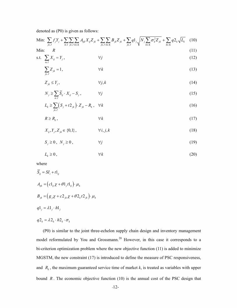
denoted as (P0) is given as follows:
Min: 21 2
j j ijk ij jk jk jk j j k jk k kj J i I j J k K j J k K j J k K k K
f Y A X Z B Z q N Z q L (10)
Min: R (11)
s.t. ij ji I
X Y
, j (12)
1jkj J
Z
, k (13)
jk jZ Y , ,j k (14)
j ij ij ji I
N S X S , j (15)
2
k j jk jk kj J
L S t Z R , k (16)
kR R , k (17)
, , {0,1}ij j jkX Y Z , , ,i j k (18)
0jS , 0jN , j (19)
0kL , k (20)
where
1 ij i ijS SI t
1 1 1 ijk ij j ij kA c t
2 2 2 jk j jk k jk kB g c t
1 1 1j j jq h
2 2 2k k k kq h
(P0) is similar to the joint three-echelon supply chain design and inventory management
model reformulated by You and Grossmann.20 However, in this case it corresponds to a
bi-criterion optimization problem where the new objective function (11) is added to minimize
MGSTM, the new constraint (17) is introduced to define the measure of PSC responsiveness,
and kR , the maximum guaranteed service time of market k, is treated as variables with upper
bound R . The economic objective function (10) is the annual cost of the PSC design that

-13-
accounts for the fixed and variable costs of installing DCs, transportation costs from plants to
DCs and from DCs to markets, pipeline inventory costs in DCs and markets, as well as safety
stock costs in DCs and markets. Constraints (12)-(14) define the PSC network structure, and
constraints (15) and (16) define the net lead times at the DCs and markets.
Similarly to our previous work,20 we can linearize30 the bilinear terms (products of binary
variables and continuous variables, or products of two binary variables) and reformulate the
model as problem (P1):
Min: 1 2
j j ijk ijk jk jk j j k kj J i I j J k K j J k K j J k K
f Y A XZ B Z q NZV q L (21)
Min: R (11)
s.t. Constraints (12) – (15), (17) – (20)
k jk jk jk kj J j J
L SZ t Z R , k (22)
ijk ijXZ X , , ,i j k (23)
ijk jkXZ Z , , ,i j k (24)
1 ijk ij jkXZ X Z , , ,i j k (25)
1 jk jk jSZ SZ S , ,j k (26)
Ujk jk jSZ Z S , ,j k (27)
1 1 Ujk jk jSZ Z S , ,j k (28)
1 jk jk jNZ NZ N , ,j k (29)
Ujk jk jNZ Z N , ,j k (30)
1 1 Ujk jk jNZ Z N , ,j k (31)
2
j k jkk K
NZV NZ , j (32)
0ijkXZ , , ,i j k (33)
0jNZV , j (34)

-14-
0jkSZ , 1 0jkSZ , 0jkNZ , 1 0jkNZ , ,j k (35)
where constraints (23)-(32) are introduced for the exact linearization. The bounds of the
variables are given in the constraints (36):
max max
Uj i ij ij
i I i IN SI t S , j (36.1)
maxU Uj j ij
i IS N S
, j (36.2)
max 0,max
U Uk j jk k
j JL S t R , j (36.3)
U Ujk jSZ S , 1 U U
jk jSZ S , ,j k (36.4)
U Ujk jNZ N , 1 U U
jk jNZ N , ,j k (36.5)
2
U Uj k j
k K
NZV N , j (36.6)
Thus, to balance the economics and responsiveness, we have two objective functions to be
minimized in (P1). One is the annual total PSC design cost, and the other one is the MGSTM.
In order to obtain the Pareto-optimal curve for the bi-criterion optimization problem, one of the
objectives is treated as an inequality with a fixed value for the bound which is considered as a
parameter. There are two major approaches to solve the problem in terms of this parameter.
One is to simply solve it for a specified number of points to obtain an approximation of the
Pareto optimal curve (ε-constraint method).31-34 The other one is to solve it as a parametric
programming problem,35, 36 which yields the exact solution for the Pareto optimal curve. While
the latter provides a rigorous solution approach, the former is easier to implement for MINLP
models. For this reason, we solve this multi-objective optimization problem with the
ε–constraint method.
From the economic objective (10) and constraint (16), it is easy to see that by increasing
kR the total annual cost of this PSC is reduced. Coupled with the responsiveness objective (11)
and constraint (17), we can observe that (P0) is always feasible for any value of kR . Note that
the lower bound of the left hand side of constraint (16) is zero, while the lower bound of the

-15-
right hand side of this constraint is R , which is a non-positive value. Thus, the problem has
an infinite number of optimal solutions in the continuous space. To be more specific, if *kR is
the optimal solution and we have the optimal value of variable R as * *max
kk K
R R , by
replacing the value of variables kR , k K with *R , we have * * *max
k kk K
R R R is also
a feasible and optimal solution of the problem. Therefore, we can always have an optimal
solution with
* * *max
k kk K
R R R k (37)
This property suggests that we can fix the guaranteed service times of all the markets ( kR )
to a certain value when using the ε–constraint method. In other words, objective (11) and
constraint (17) can be removed and variables kR can be treated as parameters in the solution
procedure. The lower bound of R and all the kR can be easily determined to be 0. To obtain
their upper bounds, we consider a modified objective function as follows,
Min: 1 2
j j ijk ijk jk jk j j k kj J i I j J k K j J k K j J k K
f Y A XZ B Z q NZV q L R (38)
where is a scaling parameter with sufficient small value, for instance, 0.001. By minimizing
(38) subject to all the constraints in (P1), we can determine the minimum upper bound of
variable R. Therefore, in the solution procedure, we solve problem (P1) under different
specifications of MGSTM between 0 and its upper bound to obtain an approximation of the
Pareto optimal curve.
5. Acetic Acid Supply Chain Example
To illustrate the application of our model, we consider an example taken from our previous
work20 for an acetic acid supply chain with three plants, three potential DCs and markets as
shown in Figure 5.
-16-
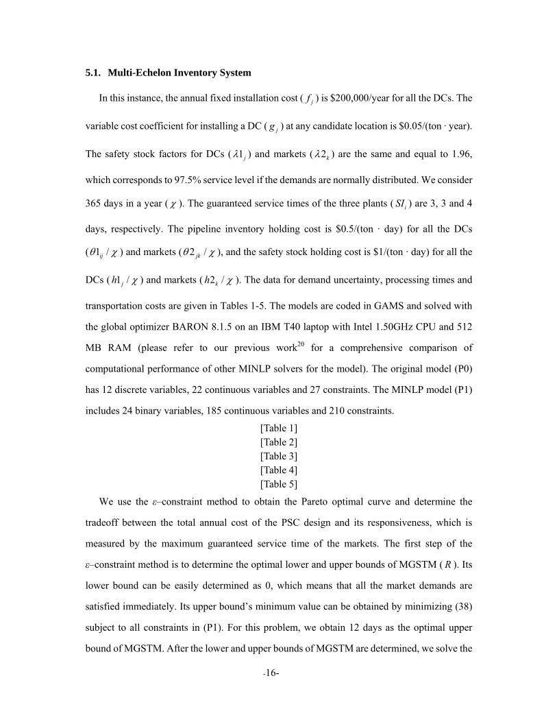
5.1. Multi-Echelon Inventory System
In this instance, the annual fixed installation cost ( jf ) is $200,000/year for all the DCs. The
variable cost coefficient for installing a DC ( jg ) at any candidate location is $0.05/(ton · year).
The safety stock factors for DCs ( 1 j ) and markets ( 2k ) are the same and equal to 1.96,
which corresponds to 97.5% service level if the demands are normally distributed. We consider
365 days in a year ( ). The guaranteed service times of the three plants ( iSI ) are 3, 3 and 4
days, respectively. The pipeline inventory holding cost is $0.5/(ton · day) for all the DCs
( 1 /ij ) and markets ( 2 /jk ), and the safety stock holding cost is $1/(ton · day) for all the
DCs ( 1 /jh ) and markets ( 2 /kh ). The data for demand uncertainty, processing times and
transportation costs are given in Tables 1-5. The models are coded in GAMS and solved with
the global optimizer BARON 8.1.5 on an IBM T40 laptop with Intel 1.50GHz CPU and 512
MB RAM (please refer to our previous work20 for a comprehensive comparison of
computational performance of other MINLP solvers for the model). The original model (P0)
has 12 discrete variables, 22 continuous variables and 27 constraints. The MINLP model (P1)
includes 24 binary variables, 185 continuous variables and 210 constraints.
[Table 1] [Table 2] [Table 3] [Table 4] [Table 5]
We use the ε–constraint method to obtain the Pareto optimal curve and determine the
tradeoff between the total annual cost of the PSC design and its responsiveness, which is
measured by the maximum guaranteed service time of the markets. The first step of the
ε–constraint method is to determine the optimal lower and upper bounds of MGSTM ( R ). Its
lower bound can be easily determined as 0, which means that all the market demands are
satisfied immediately. Its upper bound’s minimum value can be obtained by minimizing (38)
subject to all constraints in (P1). For this problem, we obtain 12 days as the optimal upper
bound of MGSTM. After the lower and upper bounds of MGSTM are determined, we solve the

-17-
problem with fixed values of R from 0 day to 12 days (e.g. 13 instances with increments of 1
day). Solving the original model (P0) with 0% optimality margin takes a total of 7,101.51 CPU
seconds for all the 13 instances. When we solve the reformulated model (P1) by minimizing
(21), the 13 instances require only 86.89 CPU seconds and the optimal solutions are the same
as what we obtained by solving model (P0).
[Figure 6] [Figure 7, (a), (b), (c)]
The results are given in Figures 6 and 7, as well as in Tables 6 and 7. The line in Figure 6 is
the Pareto optimal curve of this problem. As can be seen, the cost ranges from $1,721,685 to
$2,519,886, while the guaranteed service time ( R ) ranges from 0 days to 12 days. We can see
that the total cost decreases as the MGSTM increases. Since the MGSTM is a measure of PSC
responsiveness, we can conclude that the more responsive the PSC is, the more cost it requires.
The columns in Figure 6 show the total safety stocks in the system under different
specifications of MGSTM. As the MGSTM increases, the total safety stocks in this PSC
decrease from 2,187 tons to 0. However, the safety stock levels do not strictly decrease as
MGSTM increases, but have a “valley” when MGSTM equal to 8 and 9 days. This is due to the
change of supply chain network structure and inventory allocation decisions between DCs and
markets.
Figure 7 shows the change of the optimal network structures under different specifications
of MGSTM. We can see that the optimal network structures for most cases are the same as
shown in Figure 7(a). When MGSTM is equal to 8, 9 and 11 days, the optimal network
structures are different from the “common” one, and they are given in Figure 7(b), 7(c) and
7(d), respectively. In Figure 7(a) and 7(d), only one DC is installed and serves all the markets.
This is due to the “risk pooling” effect, which tries to group markets to be served by one DC so
as to reduce the total safety stocks. In Figure 7(b) and 7(c) there is one more DC installed that
leads to higher DC installation costs, but presumably reduces the total transportation and
inventory costs. This reveals the tradeoff between transportation cost, inventory cost and
facility location cost, and suggests that changing network structure may be more effective to
improve the PSC responsiveness compared to holding safety stock. A similar conclusion is also

-18-
presented in our previous work,5 although in that case safety stock levels always decrease as
the PSC responsiveness decreases due to the single echelon inventory model used in that
model. When the MGSTM increases from 9 days to 10 days, the optimal number of DCs
reduces from two to one, and the network structure “returns” to the one shown in Figure 7(a).
This is also presumably due to the tradeoff between the several cost items as discussed above.
When the MGSTM increases to 11 and 12 days, the optimal safety stocks in the systems reduce
to zero (as in Figure 6), and the two optimal network structures have the same distribution
network, but different production plants. The reason is that Plant1 has a shorter guaranteed
service time (3 days) than Plant 3 (4 days), but higher unit transportation cost (as in Table 4)
from the plant to DC 2. To reduce the overall transportation, inventory and supply chain design
cost, it is optimal to include Plant3 instead of Plant1 in the supply chain network when
MGSTM is 12 days. Note that these existing plants are considered to be acting as suppliers,
which can be added or removed from the supply chain network at no additional instillation
costs, although the transportation cost from plants to DCs are taken into account.
Tables 6 and 7 show the change of optimal net lead times and optimal safety stock levels in
the DCs and markets under different specifications of the maximum guaranteed service time to
the markets (MGSTM). It is interesting to note that the optimal net lead times of DCs and
markets are at integer values, although they are not restricted to be integers in the optimization
model. In the most “responsive” case, both DCs and markets hold maximum safety stock to
guarantee the MGSTM equal to zero. As the MGSTM increases, the safety stock levels and net
lead times in the markets decrease, while the safety stock levels and net lead times in the DCs
remain unchanged until the safety stocks in markets deplete. This trend shows that holding
safety stocks in the DCs (upstream) is more efficient to increase PSC responsiveness than
holding safety stocks in the markets (downstream). When the MGSTM is between 5 days and 8
days, no market holds inventory and the safety stocks in the DCs decrease as the MGSTM
increases. When the MGSTM increases to 8 and 9 days, the safety stocks are shifted from the
DCs to the Markets. The change of inventory allocation decision is presumably due to the
change of the PSC network structure as given in Figure 7(b) and 7(c), and leads to the “valley”

-19-
in the inventory profile as in Figure 6. When the MGSTM increases from 9 days to 10 days, we
can see that the safety stocks “return” to the DCs and this change further reduces the total cost
but almost double the total safety stocks. These interesting changes of inventory allocation and
the associated network structure are due to the fact that we consider the two-echelon inventory
(DCs and markets).
Although this is a small example, the proposed approach for PSC responsiveness can easily
be applied to large scale PSCs design problems by employing the tailored algorithm presented
in our previous work20. In the Appendix, we present the data and results of a large scale
instance with 10 plants, 50 potential DCs and 100 markets, by solving the MINLP model with
the Lagrangead relaxation and decomposition algorithm as discussed in our previous work.20
5.2. Single-Echelon Inventory System
To illustrate the similarities and differences of the two measures of PSC responsiveness,
MGSTM and expected lead time,5 we consider a special case that only DCs of the acetic acid
supply chain can hold safety stocks, i.e. single echelon inventory.
To model and optimize the system with the guaranteed service approach, we need to make a
few minor changes in model (P1). By fixing the values of the net lead times in the markets to
zero in model (P1), i.e. 0, kL k , model (P1) reduces to the PSC design problem with single
echelon inventory, as the markets are not allowed to hold safety stocks due to their zero net lead
times. Due to the change of the inventory structure, the optimal lower and upper bounds of the
MGSTM may change. Thus, to obtain the optimal lower bound we solve an optimization
problem by minimizing (11) subject to all the constraints in model (P1), and to obtain the
optimal upper bound we solve a problem by minimizing (38) subject to all the constraints in
model (P1).
Using expected lead time as the responsiveness measure for PSC design problem leads to
another MINLP model (Q1), the detailed formulation of which is given in the Appendix. The
major difference between this model and the one introduced in our previous work5 is that the
standardized normal variables j are restricted to be not greater than the safety stock factor

-20-
1 j , so as to be consistent to the data used in the guaranteed service time approach. Besides,
the risk-pooling effect is also taken into account in this model.
We solve these problems using the same computer described in Section 4.1. All the
instances are solved with the global optimizer LINDOGlobal in the GAMS modeling system,
since BARON does not support the error function included in model (Q1).
For the guaranteed service time case, the resulting optimal lower bound of MGSTM is 2
days, and the optimal upper bound is 12 days. Then we fix the value of R to integer values
from 2 days to 12 days, and solve these 11 instances by minimizing (21) subject to all the
constraints of (P1). The 11 instances require 228 CPU seconds. When using the expected lead
time as the measure of responsiveness, the resulting optimal lower and upper bounds of the
expected lead time are 2.125 days and 8 days, respectively. We then fix the value of T to 11
evenly distributed points ranging from 2.125 days to 8 days, and solve these 11 instances by
minimizing (38) subject to all the constraints of (Q1). The 11 instances require a total of 248
CPU seconds. The resulting Pareto-optimal curves, optimal safety stock levels, and optimal
PSC network structure under different specifications of MGSTM ( R ) and expected lead time
(T ) are given in Figures 8 – 11.
Figure 8 shows the Pareto optimal curves for this PSC with single-echelon inventory using
two different measures for responsiveness. In the Pareto curve for guaranteed service
approach, the total cost ranges from $ 1.72 MM to $ 2.41 MM, while the MGSTM ( R ) ranges
from 2 days to 12 days. We can see that total cost decreases as MGSTM increase. The trade-off
shows that the more responsive the PSC is, the more cost is required in the PSC design. In
particular, the total cost decreases significantly when MGSTM increases from 3 days to 4 days
and from 10 days to 11 days, because the optimal PSC network structure changes (see Figure
11) at these points of the Pareto curve.
In the Pareto curve for measuring responsiveness with expected lead time, the total cost
ranges from $ 1.72 MM to $ 2.35 MM, while the expected lead time ranges from 2.125 days to
8 days. We can see a similar trend as in the other curve that the total cost decreases as the
expected lead time increases. By comparing these two curves, we can see the one using

-21-
guaranteed service approach lies above the curve from the expected lead time. The reason is
that guaranteed service approach is a worst case criterion to measure the response time, while
expected lead time is a “weighted” measure that considers both the case of over-stock and the
case of stock-out. Thus, under the same total cost, the MGSTM usually has a larger value than
the expected lead time. Note that the results are consistent with the observations discussed in
Section 2.3 where we consider a PSC with fixed design. For the extreme values of these two
curves, we can see that both curves have the same minimum cost solution, which corresponds
to the case of holding zero safety stock in all the DCs, although the corresponding MGSTM is
12 days while the expected lead time is 8 days. The lower bound of the MGSTM is 2 days,
which corresponds to the maximum delivery lead time in the expected lead time approach.
However, the lower bound of the expected lead time is not 2 days but 2.125 days, because the
stockout probability is always greater than 2.5% due to the “bounded” safety stock factor
corresponding to 97.5% service level. It is interesting to see that in the most “responsive” case
( 2R days and 2.125T days), these two curves have different total costs, although the
optimal network structures are the same (Figure 11). The reason can be found from Figure 10.
We can see that DC1 has the same optimal safety stocks in these two instances, while safety
stocks in DC2 are higher in the case of using the guaranteed service. This is because both
measures somewhat consider the “worst case”. DC1 is included in the linear supply chain or
serves those markets that have dominant effect of the maximum values of R and T . Thus,
once DC1 holds the maximum safety stocks to allow MGSTM and expected lead time reach
their minimum, DC2 gains certain flexibility to hold lower safety stock than its maximum
level, while still keeping the MGSTM and expected lead time unchanged. The differences
between these two measures allow DC2 to have different levels of flexibility to reduce its
safety stocks and the associated total costs. Therefore, these two Pareto optimal curves have
different maximum total costs.
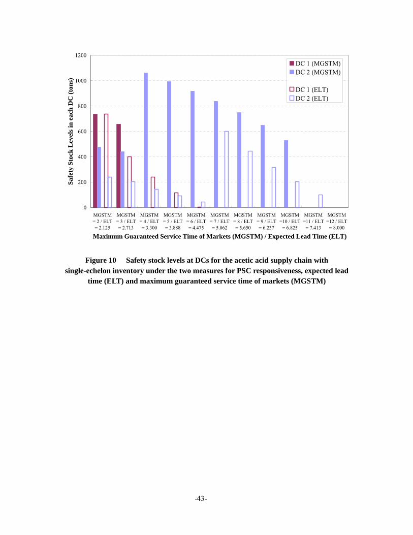
Figure 9 shows the change of total safety stock level in the PSC under two measures of
responsiveness. We can see that when the expected lead time is used as the responsiveness
measure, the total safety stock level increase significantly when the expected lead time

-22-
increases from 4.475 days to 5.062 days. The reason is that the optimal network structure
changes with a reduction of the number of DCs from two to one as the expected lead time
increases. This further reveals the trade-off between DC installation cost, transportation cost
and safety stock cost. The detailed safety stock levels in each DC using these two measures of
responsiveness are given in Figure 10, while the optimal network structures under different
specifications of responsiveness are given in Figure 11.
The comparison shows that these two measures of PSC responsiveness, MGSTM and
expected lead time, are inherently consistent. The proposed new measure, MGSTM, represents
the “worst case”, but it has the advantage that it can be applied to PSCs with multi-echelon
structure of the inventory system leading to more accurate results.
6. Conclusion
In this paper, we have proposed a new measure for PSC responsiveness based on the concept
of guaranteed service approach that allows modeling the multi-echelon stochastic inventory
system of a PSC. This measure is incorporated into a joint PSC network design and inventory
control model to tradeoff annualized PSC cost and responsiveness within a bi-criterion
optimization approach. Some special model properties of the bi-criterion MINLP optimization
model were exploited to speed up the solution for the Pareto-optimal solutions. An illustrative
example on an acetic acid supply chain was presented to illustrate the application of proposed
approach and models. In addition, comprehensive comparisons between the proposed measure
and the expected lead time, which is another measure for PSC responsiveness focus on the
single-stage inventory system, were presented. The analytical results show that these two
measures are consistent, although the proposed measure has the advantage that it can be
applied to multi-echelon inventory systems.
Acknowledgment
The authors acknowledge the financial support from the National Science Foundation under
Grants No. DMI-0556090 and No. OCI- 0750826, and the Pennsylvania Infrastructure
Technology Alliance (PITA).

-23-
Appendix:
A. Large-Scale Example for PSC Design with Multi-Echelon Inventory using MGSTM as Responsiveness Measure
We consider a large-scale acetic acid supply chain example with 10 plants, 50 potential DCs
and 100 markets. The maximum guaranteed service time of markets (MGSTM) is used as the
measure of supply chain responsiveness.
The input data of this example is given as follows. The safety stock factors for DCs ( 1j )
and markets ( 2k ) are the same and equal to 1.96, which corresponds to 97.5% service level is
demand is normally distributed. We consider 365 days in a year ( ). The guaranteed service
time of the last echelon customer demand zones ( kR ) are set to 0. The annual fixed costs
($/year) to install the DCs ( jf ) are generated uniformly on U[150,000, 160,000] and the
variable cost coefficient ( jg , $/ ton · year) are generated uniformly on U[0.01, 0.1]. The
guaranteed service times of the plants ( iSI , days) are set as integers uniformly distributed on
U[7, 10]. The order processing time ( 1ijt , days) between plants and DCs are generated as
integers uniformly distributed on U[3, 7], and the order processing time ( 2 jkt , days) between
DCs and customer demand zones are generated as integers uniformly distributed on U[2, 5].
The unit transportation cost from plants to DCs ( 1ijc , $/ton) and from DCs to customer demand
zones ( 2 jkc , $/ton) are set to 1 1 [0.05, 0.1]ij ijc t U and 2 2 [0.05, 0.1]jk jkc t U . The
expected demand ( i ,ton/day) is generated uniformly distributed on U[75, 150] and its
standard deviation ( i , ton/day) is generated uniformly distributed on U[0, 50]. The daily unit
pipeline and safety stock inventory holding costs ( 1 /ij , 2 /jk , 1 /jh and 2 /kh )
are generated uniformly distributed on U[0.1, 1].
The resulting MINLP problem includes 5,550 binary variables, 75,250 continuous variables
and 185,350 constraints. Solving this problem directly with a global optimizer is a non-trivial

-24-
task. To address the computational challenge, we employ the Lagrangean relaxation and
decomposition algorithm as discussed in our previous work,20 and integrate it with the
ε–constraint method to obtain the Pareto optimal curve and determine the tradeoff between the
total annual cost of the PSC design and its responsiveness. The first step of the ε–constraint
method is to determine the optimal lower and upper bounds of MGSTM ( R ), which are 0 days
and 18 days, respectively. Then we solve the problem with fixed values of R from 0 day to
18days (e.g. 19 instances with increments of 1 day). Solving the model (P1) takes a total of
479,563 CPU seconds for all the 19 instances.
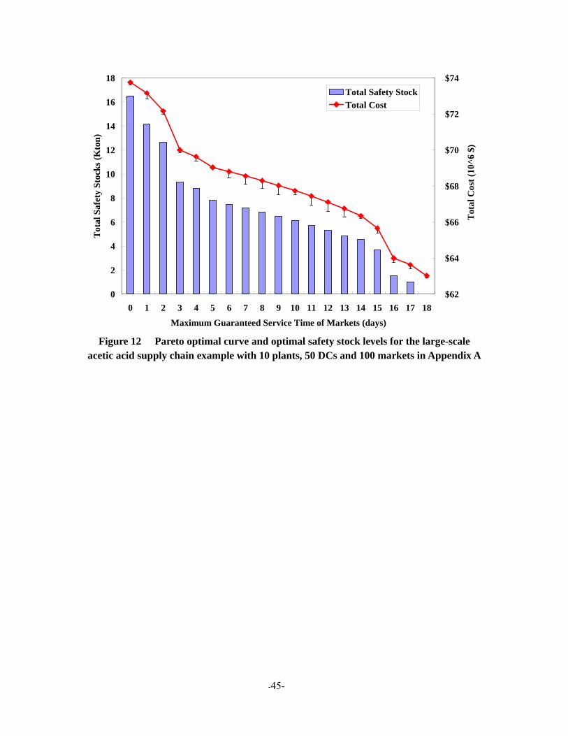
[Figure 12]
The results are given in Figures 12. The red line in Figure 12 is the Pareto optimal curve of
this problem. As can be seen, the cost ranges from $73,752,953 to $63,028,935, while the
guaranteed service time ( R ) ranges from 0 days to 18 days. We can see that the total cost
decreases as the MGSTM increases. Thus, the more responsive the PSC is, the more cost it
requires. Due to the integer variables and non-convex terms, there are duality gaps by solving
the problems with the Lagrangean relaxation and decomposition algorithm, and these gaps are
reflected on the error bars in the Pareto optimal curve. We can see that these gaps are rather
small and do not affect the trend of the Pareto optimal curve. The columns in Figure 12 show
the total safety stocks in the system under different specifications of MGSTM. As the MGSTM
increases, the total safety stocks in this PSC decrease from 6,302,893 tons to 0. It shows that
the more inventories we have, the more responsive the PSC is.
B. Model Formulation for PSC Design with Single-Echelon Inventory using Expected Lead Time as Responsiveness Measure
Using expected lead time as the measure for PSC responsiveness for the design of the acetic
acid supply chain leads to the following MINLP model (Q1):
Min: 1
j j ijk ij jk jk jk j jj J i I j J k K j J k K j J
f Y A X Z B Z h SS (39)
Min: T (40)
s.t. ij ji I
X Y
, j (12)

-25-
1jkj J
Z
, k (13)
jk jZ Y , ,j k (14)
1
j i ij iji I
U SI t X , j (41)
2
j j k j jkk K
SS U Z , j (42)
1 ( ) j jP , j (43)
2 ij ij j jk jkT S X P t Z , , ,i j k (44)
, , {0,1}ij j jkX Y Z , , ,i j k (18)
0jSS , 0jU j (45)
0 1 jP , 0 1 j j j (46)
where
1 1 1 ijk ij j ij kA c t
2 2 2 jk j jk k jk kB g c t
21(x) exp( )d
22
x xx
The objective function (39) represents the total annual cost of the PSC design. The first term
in (39) is the annual DC installation cost, the second and the third terms are the total annual
transportation and pipeline inventory cost, and the annual total safety stock cost in the DCs is
given by the fourth term, where jSS is the safety stock level in DC j . The objective function
(40) is to minimize the total expected lead time of the entire PSC (T ). jU is the replenishment
lead time of DC j , and constraint (41) defines its value. The variance of the demand over the
replenishment lead time of DC j is given by 2
k j jkk K
U Z , which takes into account the
risk-pooling effect.37 Constraint (42) shows that safety stock level ( jSS ) at DC j is equal to
the standard deviation of its demand over the lead time times the standardized normal variables

-26-
j , which is further used to define the stockout probability ( jP ) in constraint (43). In addition,
constraint (46) restricts the standardized normal variables j to be non-negative and not
greater than the safety stock factor 1 j , so as to be consistent with the data used in the
guaranteed service approach.
Note that we can similarly linearize30 the bilinear terms (products of binary variables and
continuous variables, j jkU Z and j ijP X ) with new variables jkUZ and ijPX using the
following linear inequalities:
1 jk jk jUZ UZ U , ,j k (47.1)
Ujk jk jUZ Z U , ,j k (47.2)
1 1 Ujk jk jUZ Z U , ,j k (47.3)
0jkUZ , 1 0jkUZ ,j k (47.4)
1 ij ij jPX PX P , ,i j (48.1)
ij ijPX X , ,i j (48.2)
1 1 ij ijPX X , ,i j (48.3)
0ijPX , 1 0ijPX ,i j (48.4)
In order to obtain the optimal lower bound of the expected lead time (T ), we solve problem
(Q1) by minimizing (40). Similarly, to obtain the optimal upper bound, we consider a new
objective function:
Min: 1
j j ijk ij jk jk jk j jj J i I j J k K j J k K j J
f Y A X Z B Z h SS T (49)
where is a scaling parameter with sufficient small value, for instance, 0.001. By minimizing
(49) subject to all the constraints in (Q1), we can determine the minimum upper bound of the
expected lead time (T ).
C. Nomenclature

-27-
Sets/Indices
I Set of plants (suppliers) indexed by i
J Set of candidate DC locations indexed by j
K Set of markets indexed by k
Parameters
1ijc Unit transportation cost from plant i to DC j
2 jkc Unit transportation cost from DC j to market k
jf Fixed cost of installing a DC at candidate location j (annually)
jg Variable cost coefficient of installing candidate DC j (annually)
1 jh Unit inventory holding cost at DC j (annually)
2kh Unit inventory holding cost at market k (annually)
kR Maximum guaranteed service time of market k
iSI Guaranteed service time of plant i
1ijt Processing time of DC j if it is served by plant i, including material handling time of DC j, transportation time from plant i to DC j, and inventory review period
2 jkt Processing time of market k if it is served by DC j, including material handling time of DC j, transportation time from DC j to market k, and inventory review period
k Mean demand at market k (daily)
2k Variance of demand at market k (daily)
Days per year (to convert daily demand and variance values to annual costs)
1ij Unit cost of pipeline inventory from plant i to DC j (annually)
2 jk Unit cost of pipeline inventory from DC j to market k (annually)
1 j Safety stock factor of DC j
2k Safety stock factor of market k
Binary Variables (0-1)
ijX 1 if DC j is served by plant i , and 0 otherwise
jY 1 if we install a DC in candidate site j , and 0 otherwise
jkZ 1 if market k is served by DC j , and 0 otherwise

-28-
Continuous Variables (0 to )
kL Net lead time of market k
jN Net lead time of DC j
kR Guaranteed service time of market k
R Maximum guaranteed service time of markets (measure of responsiveness)
jS Guaranteed service time of DC j to its successive markets
T Expected lead time of the PSC network (measure of responsiveness)
jSS Safety stock level at DC j
jU Replenishment lead time of DC j
j Standardized normal variable of DC j
jP Stockout probability of DC j
ijkXZ Auxiliary variable
jNZV Auxiliary variable
jkSZ Auxiliary variable
1 jkSZ Auxiliary variable
jkNZ Auxiliary variable
1 jkNZ Auxiliary variable
jkUZ Auxiliary variable
1 jkUZ Auxiliary variable
ijPX Auxiliary variable
1ijPX Auxiliary variable
References
(1) Varma, V. A.; Reklaitis, G. V.; Blau, G. E.; Pekny, J. F., Enterprise-wide modeling & optimization – An overview of emerging research challenges and opportunities. Computers & Chemical Engineering 2007, 31, 692-711. (2) Fisher, M. L., What is the right supply chain for your product? Harvard Business
Review 1997, 75, (2), 105-116. (3) Grossmann, I. E., Enterprise-wide Optimization: A New Frontier in Process Systems
Engineering. AIChE Journal 2005, 51, 1846-1857.
-29-
(4) You, F.; Grossmann, I. E., Optimal Design and Operational Planning of Responsive Process Supply Chains. In Process System Engineering: Volume 3: Supply Chain Optimization, Papageorgiou; Georgiadis, Eds. Wiley-VCH: Weinheim, 2007; pp 107-134. (5) You, F.; Grossmann, I. E., Design of Responsive Supply Chains under Demand
Uncertainty. Computers & Chemical Engineering 2008, 32, (12), 2839-3274. (6) Sabath, R., Volatile demand calls for quick response. International Journal of Physical
Distribution & Logistics Management 1998, 28, (9/10), 698-704. (7) Rotstein, G.; Shah, N.; Sorensen, E.; Macchietto, S.; Weiss, R. A., Analysis and design
of paint manufacturing processes. Computers & Chemical Engineering 1998, 22, (Supplement: Suppl. S), S279-S282. (8) Shah, N., Process industry supply chains: Advances and challenges. Computers &
Chemical Engineering 2005, 29, (6), 1225-1236. (9) Shah, N., Pharmaceutical supply chains: key issues and strategies for optimisation.
Computers & Chemical Engineering 2004, 28, (6-7), 929-941. (10) Tahmassebi, T., Issues in the management of manufacturing complexity.
Computers & Chemical Engineering 1999 23, (S), S907-S910. (11) Voudouris, V. T., Mathematical programming techniques to debottleneck the
supply chain of fine chemical industries. Computers & Chemical Engineering 1996 20, (Suppl. B), S1269-S1274. (12) Minner, S., Multiple-supplier inventory models in supply chain management: A
review. International Journal of Production Economics 2003, 81-82, 265-279. (13) Minner, S., Strategic safety stocks in reverse logistics supply chains. International
Journal of Production Economics 2001, 71, 417-428. (14) Inderfurth, K.; Minner, S., Safety stocks in multi-stage inventory systems under
different service measures. European Journal of Operations Research 1998, 106, 57-73. (15) Inderfurth, K., Valuation of leadtime reduction in multi-stage production systems.
In Operations Research in Production Planning and Inventory Control., Fandel, G.; Gulledge, T.; Jones, A., Eds. Springer: Berlin, Germany, 1993; pp 413–427. (16) Inderfurth, K., Safety Stock Optimization in Multi-Stage Inventory Systems.
International Journal of Production Economics 1991, 24, 103-113. (17) Graves, S. C.; Willems, S. P., Supply chain design: safety stock placement and
supply chain configuration. In Handbooks in Operations Research and Management Science, de Kok, A. G.; Graves, S. C., Eds. Elsevier: North-Holland, Amsterdam, 2003; Vol. 11, pp 95-132. (18) Graves, S. C.; Willems, S. P., Optimizing strategic safety stock placement in
supply chains. Manufacturing & Service Operations Management 2000, 2, (1), 68-83. (19) Graves, S. C., Safety Stocks in Manufacturing Systems. Journal of Manufacturing
and Operations Management 1988, 1, 67-101. (20) You, F.; Grossmann, I. E., Integrated Multi-Echelon Supply Chain Design with
Inventories under Uncertainty: MINLP Models, Computational Strategies. AIChE Journal 2008, Submitted.

-30-
(21) You, F.; Grossmann, I. E., Mixed-Integer Nonlinear Programming Models and Algorithms for Large-Scale Supply Chain Design with Stochastic Inventory Management. Industrial & Engineering Chemistry Research 2008, 47, (20), 7802. (22) Zipkin, P. H., Foundations of Inventory Management. McGraw-Hill: Boston, MA,
2000. (23) Graves, S. C.; Willems, S. P., Optimizing the supply chain configuration for new
products. Management Science 2005, 51, (8), 1165-1180. (24) Little, J. D. C., A Proof of the Queueing Formula L = λ W. Operations Research
1961, 9, 383-387. (25) Christopher, M.; Towill, D., An integrated model for the design of agile supply
chains. International Journal of Physical Distribution & Logistics Management 2001, 31, (235-246). (26) Holweg, M., The three dimensions of responsiveness. International Journal of
Operations & Production Management 2005, 25, 603-622. (27) Savelsbergh, M.; Song, J.-H., Inventory routing with continuous moves
Computers & Operations Research 2007, 34, (6), 1744-1763 (28) Campbell, A. M.; Clarke, L. W.; Savelsbergh, M. W. P., Inventory Routing in
Practice. In The Vehicle Routing Problem, Toth, P.; Vigo, D., Eds. SIAM: Philadelphia, PA, USA, 2001; pp 309-330. (29) Hübner, R., Strategic Supply Chain Management in Process Industries: An
Application to Specialty Chemicals Production Network Design. Springer-Verlag: Heidelberg, 2007. (30) Glover, F., Improved Linear Integer Programming Formulations of Nonlinear
Integer Problems. Management Science 1975, 22, (4), 455-460. (31) Mitra, K.; Gudi, R. D.; Patwardhan, S. C.; Sardar, G., Midterm supply chain
planning under uncertainty: A multiobjective chance constrained programming framework. Industrial & Engineering Chemistry Research 2008, 47, (15), 5501-5511. (32) Chen, C.-L.; Lee, W.-C., Multi-objective optimization of multi-echelon supply
chain networks with uncertain product demands and prices. Computers & Chemical Engineering 2004, 28, 1131-1144. (33) Cheng, L.; Subrahmanian, E. W., A. W., Multi-objective decisions on capacity
planning and production - Inventory control under uncertainty Industrial & Engineering Chemistry Research 2004 43, (9), 2192-2208. (34) Raj, T. S.; Lakshminarayanan, S., Multiobjective optimization in multiechelon
decentralized supply chains. Industrial & Engineering Chemistry Research 2008, 47, (17), 6661-6671. (35) Dimkou, T.; Papalexandri, K., A parametric optimization approach for
multiobjective engineering problems involving discrete decisions. Computers & Chemical Engineering 1998, 22, (S), S951-S954. (36) Dua, V.; Pistikopoulos, E., Parametric Optimization in Process Systems
Engineering: Theory and Algorithms. Proceedings of the Indian National Science Academy 2003, 69, (3-4), 429-444.
-31-
(37) Eppen, G., Effects of centralization on expected costs in a multi-echelon newsboy problem. Management Science 1979, 25, (5), 498-501.

-32-
Figure Captions
Figure 1 Inventory system controlled by base stock policy Figure 2 Conceptual relationship between PSC responsiveness and maximum guaranteed service time of the last echelon Figure 3 Network structure and processing times of the illustrative example Figure 4 Probability distribution of the uncertain demands in the illustrative example Figure 5 Acetic acid supply chain network superstructure Figure 6 Pareto optimal curve and optimal safety stock levels for the acetic acid supply chain example
Figure 7 Optimal acetic acid supply chain network structure under different maximum guaranteed service time of markets (multi-echelon inventory case)
(7a) Optimal network for maximum guaranteed service time of markets is 0-7 or 10, 12 days (7b) Optimal network for maximum guaranteed service time of markets is 8 days (7c) Optimal network for maximum guaranteed service time of markets is 9 days (7d) Optimal network for maximum guaranteed service time of markets is 11 days
Figure 8 Pareto optimal curve for the acetic acid supply chain with single-echelon inventory for expected lead time and maximum guaranteed service time of markets
Figure 9 Total safety stock levels for the acetic acid supply chain with single-echelon inventory under the two measures for PSC responsiveness, expected lead time and maximum guaranteed service time of markets
Figure 10 Safety stock levels at DCs for the acetic acid supply chain with single-echelon inventory under the two measures for PSC responsiveness, expected lead time (ELT) and maximum guaranteed service time of markets (MGSTM)
Figure 11 Optimal acetic acid supply chain network structure (with single-echelon inventory) under different specifications of maximum guaranteed service time of markets (MGSTM) and expected lead time (ELT)

-33-
(11a) Optimal network for MGSTM = 2, 3 days, ELT = 2.125, 2.713, 3.300, 3.888, 4.475 days (11b) Optimal network for MGSTM = 4 - 10, 12 days, ELT = 5.062, 5.650, 6.237, 6.825, 7.413, 8 days (11c) Optimal network structure for MGSTM = 11 days,
Figure 12 Pareto optimal curve and optimal safety stock levels for the large-scale acetic acid supply chain example with 10 plants, 50 DCs and 100 markets in Appendix A

-34-
Time
Inve
ntor
y
Lead time l
Place order
Receive order
Base-Stock Level S
Review period p
Inventory position
Inventory on hand
Safety Stock
Pipeline Inventory
Figure 1 Inventory system controlled by base stock policy

-35-
PSC Responsiveness
Maximum Guaranteed Service Time of Last Echelon
Figure 2 Conceptual relationship between PSC responsiveness and maximum guaranteed service time of the last echelon

-36-
Figure 3 Network structure and processing times of the illustrative example

-37-
Pro
babi
lity
µ Demand
Stockout
Safety Stock
Figure 4 Probability distribution of the uncertain demands in the illustrative example

-38-
Figure 5 Acetic acid supply chain network superstructure

-39-
0
500
1000
1500
2000
2500
0 1 2 3 4 5 6 7 8 9 10 11 12
Maximum Guaranteed Service Time of Markets (days)
Tot
al S
afet
y S
tock
s (t
ons)
$1.60
$1.80
$2.00
$2.20
$2.40
$2.60
Tot
al C
ost
(10^
6 $)
Total Safety Stock
Total Cost
Figure 6 Pareto optimal curve and optimal safety stock levels for the acetic acid supply
chain example

-40-
(a) Optimal network for maximum guaranteed service time of markets is 0-7 or 10, 12 days
(b) Optimal network for maximum guaranteed service time of markets is 8 days
(c) Optimal network for maximum guaranteed service time of markets is 9 days
(d) Optimal network for maximum guaranteed service time of markets is 11 days
Figure 7 Optimal acetic acid supply chain network structure under different maximum guaranteed service time of markets (multi-echelon inventory case)

-41-
1.70
1.80
1.90
2.00
2.10
2.20
2.30
2.40
2.50
1 2 3 4 5 6 7 8 9 10 11 12 13
Tot
al C
ost
(10^
6 $)
Measured by Maximum Guaranteed ServiceTime of Markets (MGSTM)Measured by Expected Lead Time (ELT)
Maximum Guaranteed Service Time of Markets / Expected Lead Time (days)
Figure 8 Pareto optimal curve for the acetic acid supply chain with single-echelon inventory for expected lead time and maximum guaranteed service time of markets

-42-
0
200
400
600
800
1000
1200
1400
MGSTM= 2 /
ELT =2.125
MGSTM= 3 /
ELT =2.713
MGSTM= 4 /
ELT =3.300
MGSTM= 5 /
ELT =3.888
MGSTM= 6 /
ELT =4.475
MGSTM= 7 /
ELT =5.062
MGSTM= 8 /
ELT =5.650
MGSTM= 9 /
ELT =6.237
MGSTM=10 /
ELT =6.825
MGSTM=11 /
ELT =7.413
MGSTM=12 /
ELT =8.000
Tot
al S
afet
y S
tock
s in
the
PSC
(ton
s)Measured by Maximum Guaranteed ServiceTime of Markets (MGSTM)Measured by Expected Lead Time (ELT)
Maximum Guaranteed Service Time of Markets (MGSTM) / Expected Lead Time (ELT)
Figure 9 Total safety stock levels for the acetic acid supply chain with single-echelon inventory under the two measures for PSC responsiveness, expected lead time and
maximum guaranteed service time of markets
-43-
0
200
400
600
800
1000
1200
MGSTM= 2 / ELT= 2.125
MGSTM= 3 / ELT= 2.713
MGSTM= 4 / ELT= 3.300
MGSTM= 5 / ELT= 3.888
MGSTM= 6 / ELT= 4.475
MGSTM= 7 / ELT= 5.062
MGSTM= 8 / ELT= 5.650
MGSTM= 9 / ELT= 6.237
MGSTM=10 / ELT
= 6.825
MGSTM=11 / ELT
= 7.413
MGSTM=12 / ELT
= 8.000
Saf
ety
Sto
ck L
evel
s in
eac
h D
C (
ton
s)DC 1 (MGSTM)DC 2 (MGSTM)
DC 1 (ELT)DC 2 (ELT)
Maximum Guaranteed Service Time of Markets (MGSTM) / Expected Lead Time (ELT)
Figure 10 Safety stock levels at DCs for the acetic acid supply chain with single-echelon inventory under the two measures for PSC responsiveness, expected lead
time (ELT) and maximum guaranteed service time of markets (MGSTM)

-44-
(a) Optimal network for MGSTM = 2, 3 days, ELT = 2.125, 2.713, 3.300, 3.888, 4.475 days
(b) Optimal network for MGSTM = 4 - 10, 12 days, ELT = 5.062, 5.650, 6.237, 6.825, 7.413, 8
days
(c) Optimal network structure for MGSTM = 11 days,
Figure 11 Optimal acetic acid supply chain network structure (with single-echelon inventory) under different specifications of maximum guaranteed service time of
markets (MGSTM) and expected lead time (ELT)
-45-
0
2
4
6
8
10
12
14
16
18
0 1 2 3 4 5 6 7 8 9 10 11 12 13 14 15 16 17 18
Maximum Guaranteed Service Time of Markets (days)
Tot
al S
afet
y S
tock
s (K
ton
)
$62
$64
$66
$68
$70
$72
$74
Tot
al C
ost
(10^
6 $)
Total Safety Stock
Total Cost
Figure 12 Pareto optimal curve and optimal safety stock levels for the large-scale
acetic acid supply chain example with 10 plants, 50 DCs and 100 markets in Appendix A

-46-
Table 1 Parameters for demand uncertainty for Illustrative Example
Mean demand i (ton/day) Standard Deviation i (ton/day)
Market1 250 150 Market2 180 75
Market3 150 80
Market4 160 45
Table 2 Order processing time ( 1ijt ) between plants and DCs (days) for Illustrative
Example
DC1 DC2 DC3
Plant1 4 4 2 Plant2 2 4 3
Plant3 3 4 4
Table 3 Order processing time ( 2 jkt ) between DCs and markets (days)
Market1 Market2 Market3 Market4
DC1 2 2 3 3 DC2 4 4 1 1
DC3 4 4 3 3
Table 4 Unit transportation Cost ( 1ijc ) from plants to DCs ($/ton)
DC1 DC2 DC3
Plant1 1.8 1.6 2.0 Plant2 2.4 2.2 1.3
Plant3 2.0 1.3 2.5
Table 5 Unit transportation Cost ( 2 jkc ) from DCs to markets ($/ton)
Market1 Market2 Market3 Market4
DC1 1.0 3.3 4.0 7.4 DC2 1.0 0.5 0.1 2.0
DC3 7.7 7.3 5.1 0.1

-47-
Table 6 Optimal net lead times (days) of DCs and markets under different specifications of maximum guarantee service time of markets (MGSTM) for the
illustrative example with multi-echelon inventory systems
MGSTM DC1
(days) DC2
(days) DC3
(days) Market1 (days)
Market2 (days)
Market3 (days)
Market4 (days)
0 day --- 8 --- 4 4 1 1 1 day --- 8 --- 3 3 0 0
2 days --- 8 --- 2 2 0 0
3 days --- 8 --- 1 1 0 0
4 days --- 8 --- 0 0 0 0
5 days --- 7 --- 0 0 0 0
6 days --- 6 --- 0 0 0 0
7 days --- 5 --- 0 0 0 0
8 days 0 0 --- 0 3 0 0
9 days 0 0 --- 0 3 0 0
10 days --- 2 --- 0 0 0 0
11 days --- 0 --- 0 0 0 0
12 days --- 0 --- 0 0 0 0
Table 7 Optimal safety stock levels (tons) of DCs and markets under different specifications of maximum guarantee service time of markets (MGSTM) for the
illustrative example with multi-echelon inventory systems
MGSTM DC1 (tons)
DC2 (tons)
DC3 (tons)
Market1 (tons)
Market2 (tons)
Market3 (tons)
Market4 (tons)
0 day --- 1,059.85 --- 588.00 294.00 156.80 88.20 1 day --- 1,059.85 --- 509.22 254.61 0 0 2 days --- 1,059.85 --- 415.78 207.89 0 0 3 days --- 1,059.85 --- 294.00 147.00 0 0 4 days --- 1,059.85 --- 0 0 0 0 5 days --- 991.40 --- 0 0 0 0 6 days --- 917.86 --- 0 0 0 0 7 days --- 837.89 --- 0 0 0 0 8 days 0 0 --- 0 254.61 0 0 9 days 0 0 --- 0 254.61 0 0 10 days --- 529.93 --- 0 0 0 0 11 days --- 0 --- 0 0 0 0 12 days --- 0 --- 0 0 0 0