Predicting completion risk in PPP Projects using Big Data

Analytics

Abstract:

Accurate prediction of potential delays in PPP projects could provide valuable information relevant for planning, and mitigating completion risk in future PPP projects. However, existing techniques for evaluating completion risk remain incapable of identifying hidden patterns in risk behaviour within large samples of projects, which are increasingly relevant for accurate prediction. To effectively tackle this problem in PPP projects, this study proposes a Big Data Analytics (BDA) predictive modelling technique for completion risk prediction. With data from 4294 PPP project samples delivered across Europe between 1992 and 2015, a series of predictive models have been devised and evaluated using linear regression, regression trees, random forest, support vector machine and deep neural network for completion risk prediction. Results and findings from this study reveal that random forest is an effective technique for predicting delays in PPP projects, with lower average test predicting error than other legacy regression techniques. Research issues relating to model selection, training and validation are also presented in the study.

Keywords: Big Data; Completion Risk; Forecasting, Public Private Partnerships (PPP); Benchmark; Predictive Modelling.

1

1 Background

In recent decades, the construction industry has been caught up in the frenzy of the widespread digital revolution that is shaping global landscape (Bilal et al., 2015). More than ever, the industry is witnessing an era of vast accumulation of valuable data needed for making informed decisions (Bilal et al., 2015). The rising availability of electronic data in diverse formats (multi-dimensional (n-D) CAD data, 3D geometric encoded data, graphical data, video, audio, text, etc.) and sizes (terabytes, petabytes etc.) has intensified the adoption of fast technologies with strong analytical capabilities within construction industry (Caldas et al., 2002). One of these frontier technologies is Big Data. Big Data are enormously large dataset that may be analysed computationally to uncover hidden patterns, unknown correlations, trends or preferences (Sagiroglu and Sinanc, 2013). Typically, Big Data has three essential attributes, also known as the 3Vs, which distinguishes it from traditional data sets (Wu et al., 2014). These are (1) Volume (Terabyte, Petabyte, Exabyte etc.); (2) velocity (continuous data streams and fast processing) and, (3) variety (disparate datasets in graphics, texts, pictures, audio, video, graphs etc.). These 3Vs are clearly apparent in most construction project data in recent times, providing opportunities for unravelling useful information from large data sample.

With robust analytical and data mining capabilities, Big Data conducts advanced analytics such as Inferential Analytics, Predictive Analytics, Prescriptive Analytics and Descriptive Analytics (Ohlhorst, 2012; Talia, 2013; Hu et al., 2014). While inferential analytics focuses on the interactions of explanatory variables with the target variable in the dataset (LaValle et al., 2012), descriptive analytics examines what is happening now based on historical data (Wu et al., 2014). Predictive analytics is concerned with prediction of future probabilities, trends and patterns within a dataset (Sagiroglu and Sinanc, 2013), while prescriptive analytics adopts optimization and simulation algorithms to propose best

2

possible outcomes and solution (Boyd and Crawford, 2012). In this study, we examine predictive modelling of completion risk in PPP projects using big data analytics. Gatzert and Kosub (2016) described completion risk in construction projects as the uncertainty that a project will be completed at a contractually agreed date. Recent literatures have examined completion risk analysis in PPP projects using various statistical tools such as Monte Carlo simulation, stochastic method, linear modelling, Project Evaluation Review Technique (PERT), critical path method etc.( Kokkaew and Chiara, 2010; Ching, 2014; Le-Hoai et al., 2008). Despite their immense contributions, most studies have concentrated on few project samples and limited data sources from simple relational databases (Soibelman et al. 2008; Kokkaew and Chiara, 2010; Javed et al., 2013). As such, these studies have either been adjudged deterministic or fixated on identifying generic factors influencing project delay (Kokkaew and Chiara, 2010). This is a major flaw in current completion risk analysis tools, as they remain incapable of identifying hidden patterns and trends in completion risk behaviour that are relevant for accurate forecasting of completion risk across large portfolio of PPP projects. The adoption of Big Data enabled predictive modelling techniques is therefore imperative for accurate prediction of completion risk within this context. These predictive techniques will enable in-depth investigation of the dynamic interaction of underlying factors influencing project delay. In this regard, high precision analytics techniques such as Deep Neural Network (ANN), Random Forest, Support Vector Machine (SVM), Linear Regression, and Regression Trees will be adopted for predictive purposes. The overarching aim of this study is therefore to develop the best Big Data Analytics based predictive model that can be used to estimate delay in PPP projects. In order to achieve the above aim, the following objectives have been identified for the study:

(1)To identify the factors influencing delay in PPP projects and their dynamic interaction in large project samples.

(2)To use advanced Big Data Analytics techniques to predict completion risk in large portfolio of PPP projects

3

(3)To compare and contrast the predictive performance of these techniques toward completion risk forecasting in large project samples.

This study seeks to examine the behaviour of completion risk across large PPP project portfolio. Using big data driven predictive analyses, 4294 PPP projects between year 1992 and 2015 were examined across Europe for completion risk prediction. Section 2 of this study focused on literature review and examines the application of Big Data Analytics in construction projects, smart cities and IOT. Existing techniques for completion risk evaluation in PPP projects were also discussed under the same section. While section 3 presents the research methodological framework for the study; Section 4 presents analysis of various predictive models for estimating completion risk in PPP projects. This is then followed by the implication for practice, while the last section concludes the study.

2 Literature Review

2.1 Big Data Analytics for Construction Projects and Smart Cities

The introduction of Building Information Modelling (BIM) has helped fast-track the generation of humongous construction data across domains such as design data, Enterprise Resource Planning (ERP) systems, project schedules, financial data, and contract data among others. Many of these datasets exist in disparate formats including 3D Geometric encoded (BIM), DXF (drawing exchange format), ifcFXML (Industry Foundation Classes XML), DWG (drawing data), DOC, XLS, PPT (Microsoft format), RVT (short for Revit), DGN (short for design), JPEG (image format), RM/MPG (video format) etc. With the emergences of sensors and embedded devices allowing facilities to generate real-time data in large volumes, variety and under high velocity (a.k.a 3V’s), the construction industry has been pushed into the Big Data era. Noticeably, despite the euphoria about Big

4

Data Analytics in the construction sector, academic literature on the topic is only gradually intensifying.

However, a quick review of construction literature revealed two emergent themes of Big Data application in the construction sector namely: Waste Analytics or Waste Management and Smart Cities vis-à-vis IOTs (Internet of Things). Lu et al. (2015) in an investigation into construction waste performance in Hong Kong developed robust KPIs for benchmarking waste generation rate using data from waste disposal records of 5764 projects. The study found demolition works as the largest contributor to waste in Hong Kong, with new building, renovation and maintenance contributing the least amount of waste to landfill. In another relevant literature Bilal et al. (2016) bemoaned existing intelligence-based waste management softwares as lacking the necessary ability to encourage stakeholders. The study also challenged the inappropriate classification of most wastes as mixed wastes under the existing waste management approaches. The study proposed a new Big Data architecture for designing-out waste from projects (by integrating Spark with BIM), and leveraged data from over 200,000 waste disposal records from 900 UK projects. Similarly, Chen et al. (2016) conducted a comparative analysis of construction waste management performances in public and private projects under similar waste management governance. The study analysed over 2 million waste disposal data from 5700 projects and concluded that construction contractors perform better on waste minimization when working on public projects than on private projects. In addition, Brown et al. (2011) investigated the readiness of the construction sector for the adoption of Big Data Analytics using sentiment analysis. Other relevant studies on Big Data in construction and engineering projects include Hampton et al. (2011), Bilal et al. (2015) and Wu et al. (2016).

Conversely, Big Data Analytics along with the wide adoption of embedded devices in hard infrastructures have also intensified discussions on Smart Cities and Internet of Things -IOT (Zanella et al., 2014; Centenaro et al.,

5

2016). Chiang and Zhang (2016) described smart cities as urban locations that use advanced communication technologies to collect and leverage electronic data via sensing devices. Through sensors, physical objects are able to stay connected through the internet and transmit data online (IOT) in way that helps manage public assets, improve operational and resource efficiency (Scuotto et al., 2016). Within the construction sector, smart cities and IOT have become a new and exciting area attracting noticeable research interests (Rathore et al., 2016; Memos et al., 2018; Gaur et al., 2015; Scuotto et al., 2016). For instance, whilst Bibri (2018) examined the state-of-the-art sensor-based big data application that are enabled for IOT in a sustainable environment, Osman (2018) investigated the necessary attributes of big data analytics algorithms suitable for developing city level smart information services. Also, in a new study done by Rathore et al. (2018) on exploiting IOT and big data analytics, sensors deployment at smart home, smart parking, surveillance, weather, vehicular networking etc. were used to collate real-time data for developing a smart digital city service including graphically represented smart transport system. In addition, Alshawish et al. (2016) demonstrated practical applications of big data in a smart city under real life situations including smart energy, smart traffic systems and smart public safety, by reviewing big data algorithms, city data collection, analysis and optimization protocols. Similarly, Ming et al. (2018) analysed the intentions behind smart city development in a city using Taiwan as a context and proposed a hierarchical model of smart city systems and data flow platform that leverages city sensor devices. However, while other studies have continued to examine Big data, IOT and smart cities within construction and engineering literature (Chakrabarty and Engels, 2016; Wu et al., 2016; Gaur et al., 2015; Scuotto et al., 2016), there remains a dearth of relevant literature leveraging data from PFI/PPP projects on big data application despite the significant public resources involved.

6

2.2 Existing Techniques for Evaluating Completion Risk in PPP Projects

Earlier studies have examined completion risk in PPPs including Kokkaew and Chiara (2010); Fight (1999); André Kik (2013); Ye and Tiong (2003); Hoffman (2008). Fight (1999 pp.9) defines completion risk as “the risk that projects do not yield (sufficient) revenues as a consequence of time and budget overruns”. Similarly, Kokkaew and Chiara (2010) refer to completion risk as the uncertainty of construction completion. For the purpose of this study, completion risk is considered as the uncertainty that a project will be completed at a contractually agreed deadline (Project Delay). Many literatures (i.e. Tam et al., 2004; Hoffman, 2008; Shane et al., 2009; Javed et al., 2013) have attributed completion risk to a number of factors within the construction process such as defective design of project, delayed access to project site, shortage in skilled labour etc. Additionally, studies have suggested a number of techniques for completion risk evaluation in construction projects (Ye and Tiong, 2003; Jannadi and Almishari, 2003; Kokkaew and Chiara, 2010; Ching, 2014; Le-Hoai et al., 2008). For instance, Ye and Tiong (2003) argued for the use of incentive schemes (bonuses) to project participants towards ensuring timely completion. The incentive scheme was assumed a function of time and other factors (such as complexity of project, source of revenue etc.), and calculated thus:

B (t , λ1 , λ2 ,R )= λ1R (T s−t )(0≤ t<T s)λ2R (T s−t )(T s≤ t<∞)

(1)

λ1R (T s−t )λ2R (T s−t )

(0≤t<T e)(T e≤ t<T s)

(2)

B (t , λ1 , λ2 ,R )=¿ λ2R (T s−t ) (T s≤ t<T1 )

λ2R (T s−T 1 ) (T1≤t<∞ )

The immense contribution of the US navy in 1950s also saw the development of a tool for planning and coordinating large-scale projects, known as Programme Evaluation Review Technique (PERT). PERT presents network diagram that provides a visual depiction of the critical paths in a

7

project schedule and the sequence in which they must be completed. PERT is calculated as:

Meandurationof activity i→ μi={ai+4mi+b i6 }

Variance of activity i→Var i={bi−ai6 }

Meanof critical path→ μ=∑j∈C

μ j ,

where C is aset of critical activities

Variance of critical path→∑j∈C

Var j ,

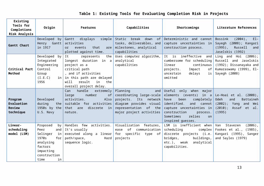
Other completion risk analysis techniques have also been proposed such as Linear-scheduling model (LSM), Critical Path Method (CPM), Gantt Chart, Vertical Production Method (VPM), Line of Balance (LOB) etc. However, despite their wide adoption overtime, André Kik, (2013) argued the reliability of current risk analyses techniques, with their associated inaccuracies regarding completion risk is limited by the use of out-dated analysis techniques (See Table 1 for Exiting techniques for Project Scheduling and Completion Risk Analysis). With the vast accumulation of project data in the construction industry, current risk analysis techniques and softwares including COMFAR III Expert (UNIDO, 1994), CASPAR (Willmer, 1991), EVALUATOR (Abdel-Aziz and Russell, 2006), and INFRISK (Dailami et al., 1999), lack the technological capabilities to hold and analyse large volumes of disparate project data at high speed. As such, a Big Data Analytics (BDA) predictive modelling of completion risk remains the realistic option.

2.3 Big Data Predictive Analytics Techniques

Big Data Analytics is predominantly employed for either inference (understanding the influence of explanatory variables over response variable) or prediction (predicting values of the response variable). Since

8

the aim of this study is twofold i.e., understanding the interactions of explanatory variables on completion risk in PPP projects (inference), as well as devising a robust completion risk prediction model (prediction), a mix of parametric and non-parametric techniques are used for predictive modelling. These techniques are discussed in depth in the subsequent sections to fulfil the purpose of this study.

9

Table 1: Existing Tools for Evaluating Completion Risk in Projects

Existing Tools for Completions Risk

AnalysisOrigin Features Capabilities Shortcomings Literature References

Gantt Chart

Developed by Henry Gantt in 1917

Gantt displays simple activitiesor events that are plotted against time.

Static break down of tasks, deliverables, and milestones, analyticalcapabilities

Deterministic and cannot capture uncertainties in construction process.

Bossink (2004), El-Sayegh (2008); Kangari (1995), Russell and Jaselskis (1992)

Critical Part Method

Developed by Integrated Engineering Control Group (I.E.C) in 1956

It represents the longest duration in a project as acritical path, and if activitiesin this path are delayed will result in the overall project delay.

Uses computer algorithm, analyticalcapabilities

It is ineffective and cumbersome for scheduling linear continuous projects. Impact of uncertain delays is omitted

Ling and Hoi (2006); Russell and Jaselskis (1992); Dissanayaka and Kumaraswamy (1999), El-Sayegh (2008)

Program Evaluation Review technique

Developed during the 1950s by the U.S. Navy

Can handle extremely large number of activities. Also suitable for activities that are discrete in nature.

Planning and coordinating large-scale projects. Its network diagram provides visual representation of the major project activities

Useful only when major elements (events) in a have been completely identified. and cannot capture uncertainties in construction process. Sometimes relies on inspired guesses.

Le-Hoai et al. (2008), Odeh and Battaineh (2002); Yang and Wei (2010); Assaf et al. (1995)

Linear-scheduling model (LSM)

Proposed by Peer and Selinger in 1970s for analysing factors impacting construction time in repetitive building projects.

Handles few activities. It’s usually executed along a linear path/space, Hard sequence logic.

Visualization features, ease of communication for specific type of projects

LSM is inefficient when scheduling complex discrete projects (i.e. bridges, buildings, etc.), weak analytical capabilities.

Van Staveren (2006), Fookes et al., (1985), Kangari (1995), Sanger and Sayles (1979)

Stochastic Critical-Path Envelope Method

Proposed by Kokkaew, N and Chiara, N (2010).

Uses simple monte Carlo simulations to randomly generate project activity durations that will later utilise CPM approach to determine project duration.

Generates a probability distribution of project duration and criticality index of project activities. Criticality index shows activity that is likely to

Lacks capacity to examine large project samples. Cannot not serve as a benchmarking tool for multiple projects.

Ng and Loosemore (2007); Shen et al. (2007); Tam and Fung (2008)

10

cause delay

Benchmarking

Many company’s In-house method of analysing completion risk

Uses completion time for similar projects to define and arrive at maximum delay time for project

Simply relies on large samples of historical data

It relies on historical data and benchmark figures that have no predictive value when considering new, large and complex projects

Chan, and Kumaraswamy (2002), Yeung et al., (2007), Bossink (2004).

11

2.3.1 Regression as the Learning Problem

When learning problem is about predicting the quantitative response, the problem is referred to as regression problem. Regression analysis involves single or multiple predictors while predictive modelling. The abstract form of regression analysis is given in Eq. 1 as

Y=ƒ ( X )+ϵ 1Where Y is quantitative response; ƒ is some fixed unknown function of predictorsX , and ϵ is some random error term that is independent of X and has a mean of zero. In Eq. 1, ƒ (X ) provides systematic information aboutY and its relationship with ρ predictors. Formally, ƒ (X ) can be expressed as shown in Eq. 2

ƒ (X )=β0+β1×x1+ β2×x2+…+β p× x p 2where x1, x2 ,…, x p represents ρ predictors andβ1 , β2 ,…, β p represents coefficients of ρ predictors and β0is intercept term. These coefficients quantify association between predictors and the response. In this study, coefficients are derived from a large array of PPP projects using various Big Data Analytics techniques. And to assess predictive performance of model, Residual sum of square (RSS) is usually employed. RSS is the square of difference of distance between predicted value (ŷ) and actual value (y). Eq. 3 describes the RSS for regression analysis.

RSS=∑i=1

n

( y i− ŷ i )2 3

Big Data Analytics functions for regression of form ƒ (X )=Ε (Y ∣ x ) tends to minimise RSS among all functions from X to Y.

This study starts predictive analysis with multivariate regression analysis as the baseline model for inferential statistics. The R function lm() is used for model development, with basic syntax as lm(y ~ x, data), where y is response, x are predictors, and data is dataset containing x and y. The summary() function retrieves the details of linear model. For attribute importance, p-values near the zero are used to identify predictors with

12

superior predictive performance. The predict() function is used to check for test error. Predicted values are plotted to visually inspect variations in predictions. Listing 1 shows R code used to perform regression analysis in this study. #Creating regression model & checking the sum of squared error for predictionslinearModel <- lm(DELAY ~ .-PROJECT, data = trainPPP)summary(linearModel)plot(linearModel)linearPredictions <- predict(linearModel, newdata = testPPP)linearPredictionsDF <- data.frame(pid = testPPP$PROJECT, pred_delay= linearPredictions, ml_func="lm")linearRSS <- sum((linearPredictions - testPPP$DELAY)^2) rssTB <- data.frame(ml_func = "lm()", rss = linearRSS)

Listing 1: R code for creating and evaluating regression analysis using lm() function

2.3.2 Regression Trees

Tree based models can be used for regression as well as classification problems. Regression trees divides the predictor space (X1 , X2 , X3 ,…, X p) into a set of non-overlapping J distinct regions (R1 ,R2, R3 ,…,R j). A regression tree follows splitting rules, starting at the root and divide down the tree into smaller subsets at each split. A regression tree comprises non-leaf and leaf nodes. Non-leaf nodes are the decision paths to be followed whereas leaf nodes contain decision values. Regions in regression tree are constructed as shapes like boxes or rectangles. Regression tree algorithm tries to find the boxes (regions) that minimize the residual sum of square, given by Eq. 4,

RSS=∑j=1

J

∑kϵ R j

( y i− ŷR j )2 ,

4

where ŷ R j is the average value of response in jth box. Since construction of

all possible boxes for a tree is computationally infeasible, greedy 13

algorithms such as recursive binary splitting are used to construct trees in a reasonable computation and time. During recursive binary splitting, every predictor X j is selected and a cut s is defined that divides predictor space into regions, yielding greatest reduction in residual sum of square. Finally, predictor X jand cut point is chosen for split among predictors (X1 , X2 , X3 ,…,∧X p) that has the lowest residual sum of square. The same process repeats for successive splits. This process of tree construction continues until stopping condition is arrived or no regions contain more than five data points. Once regions (R1 ,R2 , R3 ,…,¿R j) are defined, predictions are made for incoming data by simply using the median or mode of data in the region to which new data belong. Regression trees are simplistic, easier to interpret, and have nice graphical representation.

Complexity of regression trees bear significant impact on their predictive power. The deeper the tree, the more likely for it to over-fit test data; hence poor predictive performance. To this end, approaches like pruning regression trees comes in play, where larger tree is grown and is pruned back to obtain an optimal sub-tree. This reduction is achieved through cost complexity pruning (cp), also called as weakest link pruning. The cp considers sub-trees, index by nonnegative parameterα . Whenα=0, tree is deepest and complex. But as α starts increasing, trees with more nodes pay more prices; hence complexity gets decreasing. So as α increases from 0, branches get pruned. Cost validation is often employed to obtain an optimal value ofα in regression analysis.

In this study, recursive partitioning and regression tree (rpart) library in R is used to fit regression tree model. The size of the tree is decided by cp, which is enforced via cross validation. Regression tree is generated accordingly using train() function for different cp values. The tree model is used to check for test error using predict() function. Predicted values are plotted to visually inspect variations in predictions. Listing 2 shows R code used to achieve these steps in RStudio.#Cross validating the decision trees

14

tr.control <- trainControl(method="cv", number=10)cp.grid <- expand.grid(.cp = (0:10)*0.001)trainTreeModel <- train(DELAY ~ .-PROJECT, data = trainPPP, method="rpart", trControl=tr.control, tuneGrid = cp.grid)trainTreePredictions <- predict(trainTreeModel, newdata = testPPP)trainTreePredictionsDF <- data.frame(pid = testPPP$PROJECT, pred_delay= trainTreePredictions, ml_func="train")trainTreeRSS <- sum((trainTreePredictions - testPPP$DELAY)^2) rssTB <- rbind(rssTB, data.frame(ml_func = "train()", rss = trainTreeRSS))

Listing 2: R code for creating and evaluating regression analysis using rpart() function

2.3.3 Random Forest

Regression trees are generally not robust. A small change in data can result in a large change in the model. Non-parametric approaches such as bagging, boosting, and random forest (RF) are mostly used to overcome these limitations. We limit our discussions to RF only. RF improves performance of regression trees by compromising interpretability, i.e., by growing many treesƒ̂1 ( x ) , ƒ̂2 (x ) , ƒ̂3 (x ) ,…,ƒ̂B ( x ), and then using average of predictions to obtain low-variance regression model, given by

ƒ̂avg ( x )= 1B∑

b=1

B

ƒ̂b ( x )5

where B denotes the number of trees. RF grows tree by considering a subset m out of ρ predictors. The rule of thumb is to choosem≈√ p predictors. RF with small m favours scenarios, with many correlated predictors.

In this study, we employed random forest to see if they improve predictive performance by growing 500 trees. We used randomForest() function to

15

grow trees on training data set. The RF model is used to check for test error using predict() function. Predicted values are plotted to visually inspect variations in predictions. Listing 3 shows R code used to model development and evaluation.#Building the random forest of trees for predicting riskforestModel <- randomForest(DELAY ~ .-PROJECT, data = trainPPP, mtry=4, importance=TRUE, ntree = 500)summary(forestModel)plot(forestModel)importance(forestModel)varImpPlot(forestModel)forestPredictions <- predict(forestModel, newdata = testPPP)forestPredictionsDF <- data.frame(pid = testPPP$PROJECT, pred_delay = forestPredictions, ml_func="randomForest")forestRSS <- sum((forestPredictions - testPPP$DELAY)^2) rssTB <- rbind(rssTB, data.frame(ml_func = "randomForest()", rss = forestRSS))

Listing 3: R code for creating and evaluating regression analysis using randomForest() function

2.3.4. Support Vector Machine (SVM)

SVM is an ML algorithm with robust regularisation capabilities to generalise to the unseen data with a high degree of accuracy. SVM models can be used for both classification and regression analysis to solve complex and real-world problems. SVM outperforms on data with many attributes even if there are a small number of training examples.

SVM works on a kernel function that transforms input data into a high dimensional space and then finds the optimal solution to the problem. The kernel functions can be linear as well as Gaussian. Linear kernels translate to linear equations and suits multi-attribute training data. The Gaussian

16

kernels convert training data into points in n-dimensional space and construct numerous linear equations using nonlinear boundaries within the kernel space.

SVM uses epsilon-intensive loss function for regression analysis. The algorithm works by finding a function where more data points lie inside the epsilon-wide insensitivity tube. The epsilon can be customized through SVM settings. SVM balances the margin of error with model robustness to achieve best generalisation for the unseen data.

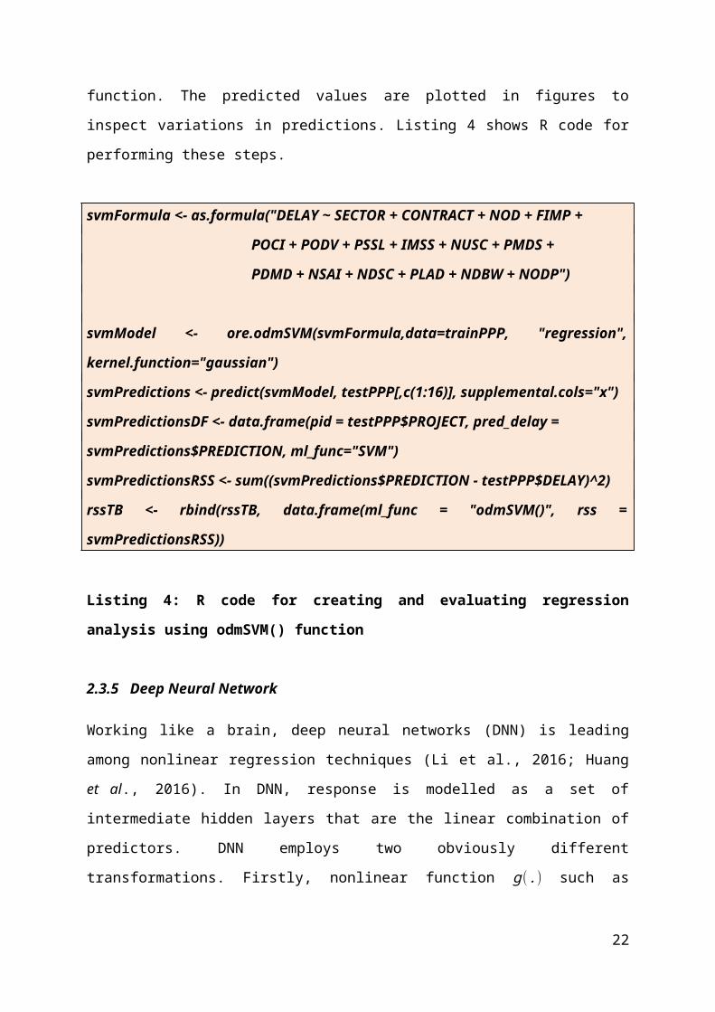
We used ore.odmSVM() to develop SVM model for regression analysis in this study. Automatic data preparation capabilities of ORE are used for one-hot encoding of categorical variables. The model is trained on training data and evaluated using test data utilizing the ore.predict() function. The predicted values are plotted in figures to inspect variations in predictions. Listing 4 shows R code for performing these steps.

svmFormula <- as.formula("DELAY ~ SECTOR + CONTRACT + NOD + FIMP + POCI + PODV + PSSL + IMSS + NUSC + PMDS + PDMD + NSAI + NDSC + PLAD + NDBW + NODP")

svmModel <- ore.odmSVM(svmFormula,data=trainPPP, "regression", kernel.function="gaussian")svmPredictions <- predict(svmModel, testPPP[,c(1:16)], supplemental.cols="x")svmPredictionsDF <- data.frame(pid = testPPP$PROJECT, pred_delay =svmPredictions$PREDICTION, ml_func="SVM")svmPredictionsRSS <- sum((svmPredictions$PREDICTION - testPPP$DELAY)^2)

17

rssTB <- rbind(rssTB, data.frame(ml_func = "odmSVM()", rss = svmPredictionsRSS))

Listing 4: R code for creating and evaluating regression analysis using odmSVM() function

2.3.5 Deep Neural Network

Working like a brain, deep neural networks (DNN) is leading among nonlinear regression techniques (Li et al., 2016; Huang et al., 2016). In DNN, response is modelled as a set of intermediate hidden layers that are the linear combination of predictors. DNN employs two obviously different transformations. Firstly, nonlinear function g(.) such as sigmoidal is used for eliciting the nonlinearity of predictors, which is explained by Eq. 6

hk=g(β0k+∑i=1

p

x iβ jk) 6

where βcoefficients are similar to that of ordinary linear regression and β jk is the effect of jth predictor on k hidden layer. Secondly, linear transformation is applied to convert outcome back to actual values, using the following Eq. 7.

ƒ (X )=γ 0+(∑k=1

H

γ khk) 7

DNN requires parameter optimization to reduce sum of squared error. To this end, specialized numerical optimization algorithms such as back-propagation (Li et al., 2016) are used. DNN over fits mostly the relationship between predictors and response due to large coefficients, which is combatted through prematurely stopping algorithm or by using penalization techniques like weight decay. DNN tries to minimize RSS for the given value of λ using Eq. 8:

∑i=1

n

( y i−f i ( x ) ) 2+ λ∑k=1

H

∑j=0

P

β jk2 + λ∑

k=0

H

γ k2 8

18

This makes model smoother and less susceptible to over fitting. Another challenge of employing DNN in regression analysis is adverse correlation effect, which is either circumvented manually or by using techniques for feature extraction like principal component analysis (PCA).

We employed neuralnetwork() library in R to develop DNN model. Using caret() function, hyper-parameter tuning for decay size of DNN is calculated and accordingly model is developed. The DNN model is used to check for test error using compute() function. Predicted values are plotted to visually inspect variations in predictions. Listing 5 shows R code used for model development and evaluation.

#Creating the DNN modelannFormula <- as.formula("DELAY ~ SECTOR + CONTRACT + NOD + FIMP + POCI + PODV + PSSL + IMSS + NUSC + PMDS + PDMD + NSAI + NDSC + PLAD + NDBW + NODP")annModel <- neuralnet(annFormula, data=trainPPP, hidden=c(10,5),linear.output=T)annPredictions <- compute(annModel, testPPP[,c(1:16)])annPredictionsDF <- data.frame(pid = testPPP$PROJECT, pred_delay = annPredictions$net.result, ml_func="ANN")annPredictionsRSS <- sum((annPredictions$net.result - testPPP$DELAY)^2) rssTB <- rbind(rssTB, data.frame(ml_func = "neuralnet()", rss = annPredictionsRSS))

Listing 5: R code for creating and evaluating regression analysis using neuralnetwork () function

19

3 Defining Key Predictors for Completion Risk Analysis using Predictive

Modelling

In order to demonstrate Big Data analytics for completion risk forecasting, data of PPP projects between 1992 and 2015 were obtained from database of the European PPP Expertise Centre (EPEC), Monthly Statistics of Construction Building Materials and Components from UK’s Department of Business Innovation and Skills, UK’s Construction Industry Data, Health and Safety in Construction Sector Report of UK, UK’s Office of the National Statistics, European Construction Market data (Euro Area Construction data) etc. Sixteen (16) key predictors causing time overrun in projects were used for the predictive modelling of completion risk. These factors were specifically chosen due to ability to quantify them and their potential impact on delay in construction project delivery (Kokkaew and Chiara, 2010; El-Sayegh, 2008). The factors are articulated in Table 2 below.

Table 2: Key Predictors Influencing Completion Risk (Delay) in PPP Projects

Values Key Predictors Influencing

Completion Risk in PPP Projects

Sources

SECTOR Projects chosen cut across nine (9)

sectors of the economy

HM Treasury (2014), NAO (2009)CONTRAC

T

Projects were either procured via

turnkey or Design Bid Build

PartnershipsUK.org.uk

NOD Av. No of defects in a construction

project

Buchholz (2004); Teizer et al.

(2010);FIMP % fluctuation in construction material

price index

Javed et al. (2013); Tam et al. (2004)POCI % change in inflation Ahmed et al. (1999); El-Sayegh

(2008).PODV % of design variations Kangari (1995); Bossink (2004);

Tatum (1989)PSSL % shortage in skilled labor Tatum (1989); Bossink (2004);

Tatum (1987)IMSS % of inferior materials supplied to site

(should be small in value).

Odeh and Battaineh (2002); Errasti

et al., (2007)NUSC No of unforeseen site conditions Dikmen et al., (2007); Flyvbjerg et al.,

(2004)PMDS % of materials damaged on site Ching (2014); Allen and Iano (2011)PDMD % Delay in Material delivery Robinson and Scott (2009); Javed et

al. (2013)NSAI No of site Accidents and injuries Rousseau and Libuser (1997); Shen

et al. (2007)NDSC No of days for site closure Kaming et al., (1997); Moselhi et al.,

(1997)PLAD % of liquidated and ascertained

damages in projects

Mohamed (2002); Tam et al.

(2004);Tatum (1987)NDBW No of days with bad weather that

prevented site work

Tatum (1987); Harty (2005); Tatum

(1989)NODP Av. No of disputes among parties El-Sayegh (2008); Russell and

Jaselskis (1992)DELAY Delay in terms of days Shen et al. (2007); Tam and Fung

(2008)20

1. Sector: The PPP projects selected for the study cuts across nine (9) sectors namely: housing, social care, transport, defence, education, health, waste management, public buildings and others (comprising comprises prisons, leisure facilities, offices, housing, emergency services, courts etc.).

2. Contract Type: The two principal contract types adopted in all the projects analysed are fixed price turnkey and Design Bid Build. Fixed price turnkey ensures a contractor delivers project under a lump sum contract, while accepting completion risk (Hoffman, 2008). On the other hand, Design Bid Build, which is also known as the traditional procurement approach allows a client to contract separate parties for design and construction phases of the project (Bing et al., 2005).

3. Average Number of defects in a construction project: Defects in project delivery is a perennial challenge in the global construction industry. According to El-Sayegh (2008), defects in construction project contribute significantly to construction delay. This could happen as a result of defects in project design or defects due to poor communication between the design managers and the contractors (Zwikael and Ahn, 2011).

4. Percentage (%) fluctuation in construction material price Index: This is often a major concern for contractors as material price fluctuation upsets prior financial forecasts and impacts project timeline, especially where contractor has no parent company cover to bail it out in the event of financial difficulties (Javed et al., 2013).

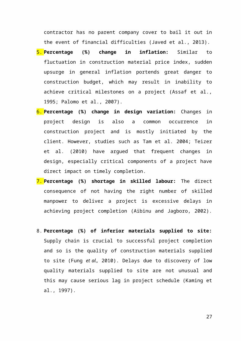
5. Percentage (%) change in inflation: Similar to fluctuation in construction material price index, sudden upsurge in general inflation portends great danger to construction budget, which may result in inability to achieve critical milestones on a project (Assaf et al., 1995; Palomo et al., 2007).

6. Percentage (%) change in design variation: Changes in project design is also a common occurrence in construction project and is mostly initiated by the client. However, studies such as Tam et al.

21

2004; Teizer et al. (2010) have argued that frequent changes in design, especially critical components of a project have direct impact on timely completion.

7. Percentage (%) shortage in skilled labour: The direct consequence of not having the right number of skilled manpower to deliver a project is excessive delays in achieving project completion (Aibinu and Jagboro, 2002).

8. Percentage (%) of inferior materials supplied to site: Supply chain is crucial to successful project completion and so is the quality of construction materials supplied to site (Fung et al., 2010). Delays due to discovery of low quality materials supplied to site are not unusual and this may cause serious lag in project schedule (Kaming et al., 1997).

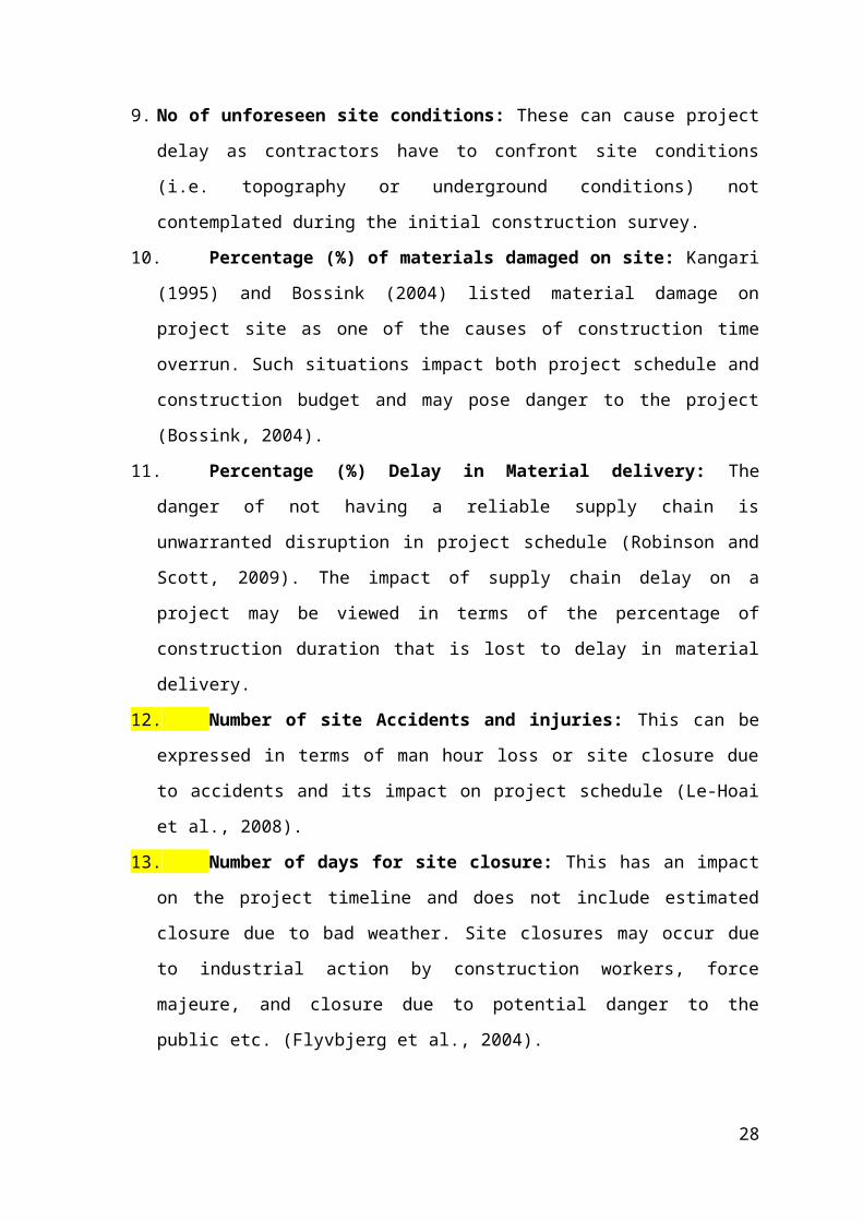
9. No of unforeseen site conditions: These can cause project delay as contractors have to confront site conditions (i.e. topography or underground conditions) not contemplated during the initial construction survey.

10. Percentage (%) of materials damaged on site: Kangari (1995) and Bossink (2004) listed material damage on project site as one of the causes of construction time overrun. Such situations impact both project schedule and construction budget and may pose danger to the project (Bossink, 2004).

11. Percentage (%) Delay in Material delivery: The danger of not having a reliable supply chain is unwarranted disruption in project schedule (Robinson and Scott, 2009). The impact of supply chain delay on a project may be viewed in terms of the percentage of construction duration that is lost to delay in material delivery.

12. Number of site Accidents and injuries: This can be expressed in terms of man hour loss or site closure due to accidents and its impact on project schedule (Le-Hoai et al., 2008).

13. Number of days for site closure: This has an impact on the project timeline and does not include estimated closure due to bad weather. Site closures may occur due to industrial action by

22

construction workers, force majeure, and closure due to potential danger to the public etc. (Flyvbjerg et al., 2004).

14. Percentage (%) of liquidated and ascertained damages in projects: Liquidated damages are financial penalties levied on contractor for breach of contractual obligations (Harty, 2005). This has negative implications for timely delivery of a project, especially where such levy is huge enough to result in financial difficulties that prevents contractor from meeting their obligations to sub-contractors (Bossink, 2004).

15. Number of days with bad weather that prevented site work: Many attimes, protracted and unpredictable weather conditions (high velocity wind, flood etc.) may prevent a project from being completed on time (Fung et al., 2010).

16. Number of disputes among parties: This may be in form of litigation or demand for contractual settlements and is a major factor which often results in project delay (Kangari, 1995). According to Teizer et al. (2010), the frequency of disputed issues on a project has negative implications for timely completion.

In this study, our goal is to develop an accurate model that can be used to estimate completion risk (project delay). In order to achieve this, we assumed a linear relationship between Completion Risk (CR) and the predictors (p). The predictors (p) are thus considered as input variables(X1 , X2 ,X3…………… .. Xρ), thereby establishing a directly proportional relationship between CR as X=(X1 , X2 ,X3⋯ Xρ). In other to achieve this, a linear model is thus developed and formally written as:

CR=f (X )+ϵ 9

Where f is a fixed unknown function of X1, X2….Xp and ϵ represents random error term, which is independent of X and has a mean of zero. In the equation above, f(X) provides systematic information about the delay in PPP projects, and could be expanded to the following equation involving multiple variables to describe this relationship:

23

f (DELAY )=β0+ β1×NOD+β2×FIMP+β3×POCI+β 4×PODV +β5×PSSL+ β6×IMSS+β7×NUSC+ β8×PMDS+β9×PDMD+ β10×NSAI+β11×NDSC+ β12×PLAD+β13×NDBW +β14× NODP

10

Where β i is the coefficients that will be estimated, where i=0 ,1 ,2,…, p employing Big Data analytics from the large array of data from PPP Project samples.

4 Research Methodology

This section explains the methodology employed in the study. After understanding the domain of completion risk in PPP projects, relevant data sources were identified to explore the most critical factors that lead to delay in PPP projects. The methodology-steps have been described in detail under subsequent sections and shown in Fig. 1 below:

Figure 1: Big Data Analytics Workflow for Predictive Risk Modelling

4.1 Databases

24

The predictive accuracy of the Big Data models depends on the quality and volume of PPP projects. Data of 4,731 PPP projects were integrated from a large number of structured and unstructured data sources. The data was distributed in a large number of data sources. These include Oracle financials, BIM models, Primavera, Candy, Health & safety, Business objects, Customer relationship management (CRM), and a large body of unstructured documents. These sources were explored to identify relevant data, structures and formats to enable the database design. Fig 2 shows types and sources of data of PPP projects used in the study. This effort has resulted in the exploration of 1.01 terabytes of data for analysis. This data fulfills all 3V’s of the Big Data that is volume, variety and velocity.

Figure 2: An overview of Big Data of PPP Projects

25

4.2 Data pre-processing and integration

Data integration task is found the toughest in the overall risk analytics experience. A variety of syntactical and semantic heterogeneities were resolved (Halevy et al. 2005; Doan & Noy 2004). To ensure data completeness, machine learning (ML) programs were used to predict missing values for predictors like average defects (Bishop 2006; Goldberg & Holland 1988). Data were standardized with vocabularies for construction sectors and contract types. Automatic conversion is augmented to deal with inappropriate interpretations especially for date columns. The data normalization is carried out by formula given in Eq. 11.

X 'i=X i−Xmin

Xmax−Xmin

11

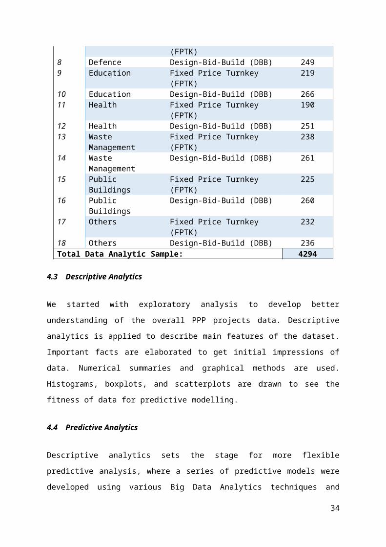
where X 'i is the scaled result of X i, X min is the smallest value of X , and X max is the largest value of X . The final data analytic sample is restricted to 4,294 PPP projects, which is eventually loaded onto Apache Spark—a resilient cluster computer engine for Big Data Analytics. Table 3 shows distribution of projects across sectors and contract types. SparkR is used for data analysis and R ggolot2 package is used for visualisation.

Table 3: Data Analytic Sample of PPP Projects used for Big Data Analytics

Sr.#. Sector Contract Type Number of

Projects1 Housing Fixed Price Turnkey (FPTK) 2002 Housing Design-Bid-Build (DBB) 2613 Social Care Fixed Price Turnkey (FPTK) 2274 Social Care Design-Bid-Build (DBB) 2505 Transport Fixed Price Turnkey (FPTK) 2336 Transport Design-Bid-Build (DBB) 2537 Defence Fixed Price Turnkey (FPTK) 2438 Defence Design-Bid-Build (DBB) 2499 Education Fixed Price Turnkey (FPTK) 21910 Education Design-Bid-Build (DBB) 266

26

11 Health Fixed Price Turnkey (FPTK) 19012 Health Design-Bid-Build (DBB) 25113 Waste

ManagementFixed Price Turnkey (FPTK) 238

14 Waste Management

Design-Bid-Build (DBB) 261

15 Public Buildings Fixed Price Turnkey (FPTK) 22516 Public Buildings Design-Bid-Build (DBB) 26017 Others Fixed Price Turnkey (FPTK) 23218 Others Design-Bid-Build (DBB) 236Total Data Analytic Sample: 4294

4.3 Descriptive Analytics

We started with exploratory analysis to develop better understanding of the overall PPP projects data. Descriptive analytics is applied to describe main features of the dataset. Important facts are elaborated to get initial impressions of data. Numerical summaries and graphical methods are used. Histograms, boxplots, and scatterplots are drawn to see the fitness of data for predictive modelling.

4.4 Predictive Analytics

Descriptive analytics sets the stage for more flexible predictive analysis, where a series of predictive models were developed using various Big Data Analytics techniques and evaluated for their predictive performance. The data are split across training and test sets using sample() function. We initially developed multivariate linear regression model to understand the interactions of predictors on response. This model is treated as the baseline model. To improve upon the predictive performance of linear model, regression trees were employed. We found different behaviour of delays across different sectors and contract types, which are not fully described by linear regression model.

Though regression trees describe non-linearity to some extent and are highly interpretable. But they are not robust; as a slight change in the data can result in a totally variant tree. To overcome these limitations in

27

predictive modelling, we employed random forest to see if they improve the predictive performance by growing 500 trees. Support vector machine (SVM) was also employed to ensure good classification of the data sample. Finally, we brought the deep learning based predictive modelling technique called deep neural networks (DNN). DNN is a black box approach that knows how to process predictors to obtain more accurate matching response. For each model, hyper-parameter tuning is performed and approaches like cross validation was employed to devise a robust model development strategy. These models were plotted using R gglot2 library for evaluating their performance in terms of decreasing the test error. It is shown that random forest is very robust and viable option to employ for estimating the completion risk in the PPP projects.

4.5 Attribute importance and ranking

Since these models employ different model development strategies, they ranked the attributes differently. To aggregate these ranking, a reliable total ranking scheme is devised. The scheme used p-value, Gini, impurity, ranked agreement factor (RAF), and percentage ranked agreement factors (PRAF) for ranking predictors for the completion risk prediction.

5 Analysis and Findings

5.1 Big Data Descriptive Analytics

We started with exploratory analysis to develop better understanding of the overall PPP project data. Descriptive analytics is the kind of first hand analysis applied to describe main features of the dataset. Important facts are elaborated to get initial impressions of data. Numerical summaries and graphical methods are often rampant. To showcase the analysis, correlation matrix plot is discussed here. Covariance test is performed to investigate multicollinearity among the 16 predictors in the dataset. In probability statistics and theory, covariance help describe the degree to which set of random variables deviate from their expected values (Newey

28

and West, 1994). According to Casella et al. (2013), positive covariance indicates positive linear relationship whereas negative values mean negative linear relationship. Covariance is calculated by the Eq. 12 and colour coded in the Fig. 3.

cov (X ,Y )=∑i=1

n (x i−x i ) ( y i− y i )n

12

Figure 3: Correlation plot depicts covariance between variables in PPP projects

As shown in Fig. 3, the bright brown slots represent the positive linear relationships whereas the blue slots depict the negative linear relationship. In addition, strong brighter colours represent the strong relationship between the variables, whereas the faded coloured regions represent independent variables. It is notable from the graph, that response variable (project delay) has strong relationship with most of the variables, which is a very good indicator for considering these variables in

29

predictive modelling. However, some variables have strong covariance, like number of days with bad weather NDBW and unforeseen site condition (UNSC). This shows collinearity issue between these variables and informs that these variables tend to add similar predictive capabilities twice. As a result, we dropped NDBW for UNSC to reduce the complexity of the model in order to achieve higher predictive performance.

5.2 Big Data Analytics for Estimating Completion Risk in PPP Projects

In the remainder of this paper, we discuss the development of predictive models for completion risk estimation. Since a single model might not be able to entirely capture the true relationship of different KPIs selected in this study with respect to delays in PPP projects, a mix of linear as well as non-linear Big Data analytics techniques are employed during model development. These techniques have really moved our understanding of completion risk to the next level. In addition, a robust completion risk estimation model is developed for assessing delays in the future PPP projects. Subsequent sections provide more details of these models and their comparisons.

5.3 Multivariate Linear Regression

An important reason behind starting with linear regression is to understand the way delay in PPP projects are influenced by myriad factors. In this case, we estimated ƒ not for the purpose of predicting completion risk in PPP projects. Instead the objective is to understand the relationship between predictor ρ and responseY or more specifically to know how Y changes as a function of ρ. So ƒ̂ is not treated as a black box rather, an elaborate description of its exact form. Listing 5 shows the summary of linear regression model.

Call:lm(formula = DELAY ~ ., data = trainPPP)

Residuals: Min 1Q Median 3Q Max

30

-0.73954 -0.07309 0.00192 0.05645 0.71047

Coefficients: Estimate Std. Error t value Pr(>|t|) (Intercept) 0.3757610 0.0172054 21.840 < 2e-16 ***SECTOR1 0.0072317 0.0105143 0.688 0.49164 SECTOR2 -0.0096546 0.0104830 -0.921 0.35714 SECTOR3 0.0005468 0.0102727 0.053 0.95755 SECTOR4 0.0100831 0.0104072 0.969 0.33270 SECTOR5 -0.0043815 0.0107594 -0.407 0.68388 SECTOR6 -0.0073937 0.0103638 -0.713 0.47565 SECTOR7 0.0018448 0.0103175 0.179 0.85810 SECTOR8 0.0103248 0.0105442 0.979 0.32757 CONTRACT1 0.0142038 0.0049633 2.862 0.00424 ** NOD 2.4175803 1.1975378 2.019 0.04361 * FIMP -0.1712855 0.0804999 -2.128 0.03344 * POCI 0.0040691 0.0076285 0.533 0.59380 PODV 0.7175872 1.1699697 0.613 0.53970 PSSL -1.1511576 0.6664203 -1.727 0.08421 . IMSS -0.4591695 0.9651310 -0.476 0.63428 NUSC 5.9326532 1.2714082 4.666 3.21e-06 ***PMDS -1.9396845 0.8848595 -2.192 0.02846 * PDMD -4.8422194 0.5106527 -9.482 < 2e-16 ***NSAI -4.1452338 1.2620944 -3.284 0.00103 ** NDSC -1.0147283 1.0164924 -0.998 0.31824 PLAD 11.3065432 1.3579018 8.326 < 2e-16 ***NDBW -6.7006330 0.5704384 -11.746 < 2e-16 ***NODP 0.0012832 0.0074467 0.172 0.86320 ---Signif. codes: 0 ‘***’ 0.001 ‘**’ 0.01 ‘*’ 0.05 ‘.’ 0.1 ‘ ’ 1

Residual standard error: 0.1283 on 2756 degrees of freedomMultiple R-squared: 0.6927, Adjusted R-squared: 0.6902 F-statistic: 270.1 on 23 and 2756 DF, p-value: < 2.2e-16

Listing 4: Summary of the Fitted Multivariate Regression Model for Risk Estimation

As mentioned earlier, sector and contract type are categorical variables, dummy variables are created automatically for each of their elements. The intercept term (β0=4.028) is implicitly added to the model. Generally, intercept term β0 is the expected delay when all predictors equal to zero. Currently the sector attribute contains 0=hospital, 1=school, 2=public building, 3=transportation, 4=housing, 5=social care, 6=defence, 7=waste, and 8=others. The model will mislead if it is applied to data set that contains sectors that are not representative within the training data

31

set. The same applies to the contract types as well. Interestingly, the model does not describe the relationship of sectors to delays, which is reported by higher p-values (0.49164, 0.35714, 0.95755, 0.33270, 0.68388, 0.47565, 0.85810, and 0.32757) of all sectors respectively. In contrast, contract type has virtually zero p-value (0.00424), which indicates strong correlation in predicting delays. The implication of this is that delay in project varies based on contract type.

The parameter estimation is computed using ordinary least squares. The Estimate column shows parameter estimation for predictors and Std. Error displays standard error associated with each of these coefficients. This is used for hypothesis testing, using t-distribution column t value, to determine if each coefficient is not statistically different from zero. And if so, then the predictor is removed from the model. Analysis show that associated hypothesis test p-value in Pr (<|t|) values are small for intercept term, contract type, number of defects (NOD), % of fluctuation in materials price (FIMP), number of unforeseen site conditions (NUSC), % materials damage (PMDS), % delay in materials delivery (PDMD), number of site injuries (NSAI), number of days bad weather (NDBW), and number of disputes among parties (NODP). Whereas, the rest of the attributes are removed from the model since they have no significance in predicting delay in PPP projects. A small p-value corresponds to small probability that such a large t value would be observed under the assumption of null hypothesis. In this case, for a given I = 0, 1, 2, …, p-1, the null and alternate hypothesis follow:

H 0 : β i=0versus H A : β i≠0

For small p-values, as is the case with above-mentioned predictors, the null hypothesis would be rejected. Whereas for rest of predictors, null hypothesis is not rejected due to large p-values of those predictors. Dropping these columns resulted in minimal changes to the estimates as well as predictive performance of the model. The last part of summary displays some of the vital details of regression model. Specifically, R2,

32

which in this context says that the model is capable to explain 69% variation in the data. And the overall p-value i.e., < 2.2e-16 is small, which indicates that null hypothesis should be rejected.

Fig. 4 shows the line plot for observed and predicted delays estimated by the linear regression where R2 is relatively good (69%). However, it is evident that the predictions are not uniformly accurate. To improve upon these, we employed regression trees to capture the non-linear behaviour of predictors on response.

Figure 4: Evaluating observed and predicted delays in the PPP projects

5.4 Regression Trees

To explain the non-linearity between the predictors and response variables, regression trees are fitted on the data of the PPP projects. Without hyper-parameter tuning, initial regression tree only considered sector variable and ignored rest of all predictors. This is quite misleading and is tackled by appropriately configuring the regression tree for risk estimation. To this end, cross validation and cost complexity pruning

33

parameters are optimised and the regression trees are grown for different cp values. Here the true power of regression trees comes into play and its effectiveness to uncover non-trivial relationship of predictors could be noticed. Contrary to linear regression, regression tree utilised majority of predictors to develop very strong risk estimation model in the dataset. Similar to regression analysis, contract type is regarded as the most superior predictor in the model; hence taken as the root of the tree. However, the second significant predictor in regression tree is considered the sector, which is totally ignored by the multivariate regression analysis. Regression tree make decisions at various levels based on the sector. So, in this case, the most complex tree is selected by the cross-validation. Fig. 5 shows the line plot for observed and predicted delays for linear regression (with accuracy improved by 79%). It is evident that predictions improved significantly. To improve upon the regression trees, we are employing regression trees to capture the non-linear behaviour of predictors on response (see Fig.6 for regression Tree Model).

Figure 5: Evaluating observed and predicted delays in the PPP project

34

Figure 6: Regression tree model for predicting delays in the PPP projects

35

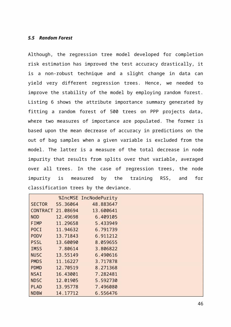
5.5 Random Forest

Although, the regression tree model developed for completion risk estimation has improved the test accuracy drastically, it is a non-robust technique and a slight change in data can yield very different regression trees. Hence, we needed to improve the stability of the model by employing random forest. Listing 6 shows the attribute importance summary generated by fitting a random forest of 500 trees on PPP projects data, where two measures of importance are populated. The former is based upon the mean decrease of accuracy in predictions on the out of bag samples when a given variable is excluded from the model. The latter is a measure of the total decrease in node impurity that results from splits over that variable, averaged over all trees. In the case of regression trees, the node impurity is measured by the training RSS, and for classification trees by the deviance. %IncMSE IncNodePuritySECTOR 55.36064 48.883647CONTRACT 21.08694 13.600641NOD 12.49698 6.409105FIMP 11.29658 5.433949POCI 11.94632 6.791739PODV 13.71843 6.911212PSSL 13.60090 8.059655IMSS 7.80614 3.806822NUSC 13.55149 6.490616PMDS 11.16227 3.717878PDMD 12.70519 8.271368NSAI 16.43001 7.282481NDSC 12.01905 5.592730PLAD 13.95778 7.496080NDBW 14.17712 6.556476NODP 12.86448 6.163925

Listing 5: Summary of the Attribute Importance by Random forest in Risk Modelling

36

Fig. 7 shows the line plot for observed and predicted delays for linear regression (with accuracy improved by 81%). It is evident that predictions improved dramatically.

Figure 7: Evaluating observed and predicted delays in the PPP projects

5.6. Support Vector Machine (SVM)

Since SVM has huge adaptability and can generalise to new data with higher accuracy, the SVM algorithm is used to train a predictive model to see its prediction capabilities. We started off with SVM for regression analysis using linear kernel, which didn't perform very well initially. The error loss was substantial. The Gaussian kernel was used which improved the model accuracy significantly. The algorithm started learning patterns into the data with respect to completion risks. For hyperparameter settings such as epsilon, manual approach was adopted at first, and different combinations of values were tested. This approach was cumbersome due to training model for every possible combination. The SVM supported automatic parameter tuning which was then used. This system-generated hyperparameter mode of SVM was found more reliable

37

and efficient since it used advanced optimisation algorithms to identify the best values to maximize model accuracy.

Monte-Carlo Sensitivity PDMD 0.092NODP 0.091NDSC 0.087PMDS 0.087PLAD 0.086FIMP 0.086NDBW 0.085NUSC 0.085PSSL 0.085IMSS 0.072NSAI 0.066POCI 0.053NOD 0.010CONTRACT 0.005PODV 0.003SECTOR 0.003

Listing 7: Summary of the Attributes Importance by SVM in Risk Modelling

SVM solved the problem by defining an n-dimensional tube around the data points to determine the vectors that yield the most extensive intervals. The coefficient vector was extracted from the SVM model to see the importance SVM was giving to each predictor for predicting the delays in PPP projects. Listing 7 above shows the attribute importance summary generated by the trained model using the Monte-Carlo Sensitivity Analysis (M-CSA). The overall accuracy of the model is 52%. Fig. 8 therefore presents the line plot for observed and predicted delays for SVM, which outperforms the linear regression but could not uplift the predictive accuracy as the tree-based models yielded for predicting the delays in the PPP projects. Although the SVM showed inadequacy in predictive power in this study, the mathematical model underpinning the algorithm suits the classification problem more than the regression analysis.

38

Figure 8: Evaluating observed and predicted delays in the PPP projects

5.7 Deep Neural Network (DNN)

Finally, to check if the deep learning technique can enhance the predictive performance of the completion risk estimation model, DNN is used. Two hidden layers of 10 and 5 nodes respectively are defined for the DNN model. The resultant model is shown in the Fig. 9. We can see that the model is not interpretable. This is because neural network is a black box methodology to predicitve modeling. It is applied in situation where the objective of the research is to make reliable predictions. So all the predictors are taken as input to the neural network. Non-linear sigmoidal transformation is done on predictors and the weights of the hidden layers are computed. These weights are eventually converted back to the linear transformation. Fig. 10 shows the line plot for observed and predicted delays for linear regression (with accuracy improved by 13%). It is evident that the predictions look very bad. This is partly due to the fact that DNN suits classification problems more than regression problems.

39

40

Figure 9: Deep neural network model for forecasting delays in the PPP projects

41

Figure 10: Evaluating observed and predicted delays in the PPP projects

5.9 Comparison of Big Data Analytics Techniques

5.9.1 Comparison based on Residual Sum of Square (RSS)

In this section, we set out to compare the 5 predictive models employed in the study using two major comparison indicators: residual sum square (RSS) and percentage rank agreement factor (PRAF). While the RSS compares the predictive performance of the model, (flexibility and interpretability were examined separately); PRAF compares each predictor’s importance in forecasting project delay. Based on results from data analysis, random forest show the least residual error, with an error margin of 1.03 and is considered good in flexibility. This is immediately followed by decision tree with RSS score of 2.17. Linear regression, support vector machine and deep neural networks however showed profound weakness in predictive performance with large error margins of 23.20, 25.64 and 469.56 between the data and the estimation models respectively. Table 4 below shows detailed comparison of the predictive

42

modelling techniques. Further details of the results are discussed in greater detail in the next section.

Table 4: Comparison of Big Data Analytics Techniques based on RSS

Big Data Analytics Techniques

RSSFlexibility

Interpretability

1 Random Forest 1.03 Good low2 Decision Tree 2.17 averag

ehigh

3 Linear Regression 23.20 Low high4 Support Vector Machine 25.64 High Low5 Deep Neural Network 469.56 High low

43

Table 5: PRAF of the Four Big Data Predictive Models and their Level of Significance (p-Value)

Sr.#.

Predictors

Ranking of Factors by Models Sum Ranks (∑)

RAF

PRAF

Overall

Ranking

Order

Linear Regression

Regression Tree

Random Forest

Support Vector

Machine

Neural Network

P-value

Rank

Gini Rank

Impurity

Rank

M-CSA

Rank

Weight

Rank1 Percentage shortage in skilled labour 0.08421 4 153.119

52 8.0596

64 0.085 9 0 0 13 0.8

169.1

11

2 Percentage Delay in Material delivery < 2e-16 1 55.2312 8 8.27137

3 0.092 1 0 0 19 1.19

54.75

23 Number of site Accidents and injuries 0.00103 2 114.301

15 7.2824

86 0.066 11 0 0 21 1.3

150.1

03

4 Percentage of design variations 0.5397 5 173.7692

1 6.91121

7 0.003 15 0 0 24 1.50

42.97

45 Percentage of liquidated and ascertained

damages in projects< 2e-16 1 41.3058

510 7.4960

85 0.086 5 0 0 26 1.6

338.2

15

6 Number of unforeseen site conditions 0.5938 5 132.5914

4 6.79174

8 0.053 12 0 0 28 1.75

33.46

67 Percentage fluctuation in construction

material price index0.00424 2 0.56240

516 13.600

62 0.005 14 0 0 29 1.8

131.0

87

8 Percent change in inflation 0.04361 3 141.6945

3 6.40911

11 0.010 13 0 0 29 1.81

31.07

89 Average number of disputes among

parties3.21E-

061 62.2733

97 6.4906

210 0.085 8 0 0 30 1.8

828.7

19

10 Number of defects in a construction project

4.48423 5 10.30915

15 48.8836

1 0.003 16 0 0 30 1.88

28.70

1011 Number of days with bad weather that

prevented site work0.03344 3 93.3244

96 5.4339

514 0.086 6 0 0 30 1.8

826.3

311

12 Percentage of materials damaged on site < 2e-16 1 21.89769

14 6.55648

9 0.085 7 0 0 32 2.00

23.95

1213 Number of days for site closure 0.02846 3 52.3381

79 6.1639

316 0.087 4 0 0 34 2.1

319.2

013

14 Projects were either procured via turnkey or Design Bid Build

0.8632 5 40.06702

11 3.71788

12 0.091 2 0 0 34 2.13

19.18

1415 Projects chosen cut across 9 sectors of the

economy0.63428 5 36.8474

212 3.8068

215 0.072 10 0 0 37 2.3

112.0

715

16 Percentage of inferior materials supplied to site

0.31824 5 22.02123

13 5.59273

13 0.087 3 0 0 42 2.63

0 16

44

5.9.2 Percentage Rank Factor

Going further, in order to have an overall agreement in the ranking of all predictors, the rank agreement factor (RAF) and PRAF (Elinwa and Joshua, 2001; Chan and Kumaraswamy, 2002) were applied. RAF and PRAF are mathematically computed using equation 13 and 14 respectively:

RAF=Σ (LR ) (RT ) (RF )(SVM )(DNN )

N 13

PRAF=RAFmax−RAF i

RAFmax×100% ,14

Where RAFmax = maximum RAF, RAF i is the RAF for criteria i, N = number of variable predictors ranked, and Σ (LR ) (RT )(RF )(SVM )(DNN ) = sum of the order of rankings of Linear Regression, Regression Trees, Random Forest, Support Vector Machine and Deep Neural Network. An absolute rank difference of 2, for example, implies more agreement as to the importance of the predictor than when the absolute rank difference is 3. The rank agreement factor may be >1, with a higher factor indicating more disagreement (Elinwa and Joshua, 2001). For the 16 predictors affecting project delay, the maximum RAFmax = 2.00. A RAF of zero implies perfect agreement. The result RAF for the models is shown in the fourteenth column of Table 5. In addition, a cursory look at results of the PRAF in Table 5 shows the five most important predictors contributing to project delay to be: (1) ‘Percentage shortage in skilled labour’, (2) ‘Percentage Delay in Material delivery, (3) ‘Number of site Accidents and injuries’, (4) ‘Percentage of design variations’, and (5) ‘Percentage of liquidated and ascertained damages in projects’. These predictors are further enumerated in the discussion section.

Additionally, the study ranked the significance of predictors under each of the five models using, P-value (linear regression), Gini (regression tree), impurity (random forest), Monte Carlo sensitivity analysis (SVM) and

45

weight (DNN). For the linear regression model, the study conducted a one-sample t-test to derive p-values for each predictor at 95% confidence level. If the mean difference is significantly different from the hypothesised value (<.05), it means that the value is statistically important in affecting project delay at the 95% confidence level (See column three and four of Table 5 for P-value of each predictor and their ranking). Going further, with regression tree, the study also evaluated the importance of some variable  when predicting   by adding up the decreases in weighted impurity for all nodes  , where  is used (averaged over all trees in the forest, but actually, we can use it on a single tree),

I (Xk )=IM∑

m∑t

N t

N∆ i( t) 15

Where the second sum is only on nodes   based on variable  . If   is Gini index, then   is called Mean Decrease Gini function. In addition, in order to identify which of the predictor variables are most important for predicting project delay in PPP projects, we used random forest to derive the mean decrease impurity importance of each predictor from assemblages of randomized trees. The ranking of each predictors derived from this process are shown in column 7 and 8 of Table 5. Regarding support vector machine, sample data were smoothly segregated based on sectors and contract types. In case of DNN, hidden layers are involved with complex interactions, hence, getting a single value for attributes is not realistic. As such, zero is set as the weight and rank of these attributes in DNN to carry out the overall ranking process.

6.0 Discussion

This section discusses results from the study and started by comparing the predictive performance of the five models (random forest, linear regression, decision tree, support vector machine and deep neural networks) in forecasting delay in PPP projects, their flexibility and interpretability respectively. Based on evidences shown in Table 4, a

46

cursory look at the residual sum of square (RSS) of the five analytical models suggest that random forest has the best predictive performance in terms of reducing error in the model to 1.23. This is followed by decision tree with RSS score of 2.17. Linear regression, support vector machine and deep neural networks however, show profound weakness in predictive performance with large error margins of 23.20, 25.64 and 469.56 between the data and the estimation models respectively. According to Theobald (1974), residual sum of square is a measure of the variability or error in the data set which is not captured in the model. A small RSS therefore suggests a tight fit of the estimation model to the data used for analysis (Tibshirani, 1996). This suggests the capability of random forest in this study to explain a greater amount of the dataset. However, considering that residual sum of square alone may not be entirely suitable to judge the correctness of the models (Al-Hazim et al., 2017), flexibility, and interpretability of the five models were also considered in the study. Although, support vector machine (SVM) and deep neural networks (DNN) showed high flexibility as evidenced in Table 4, this is only attributed to their ability to accept and review new data streaming in and thus help provide a progressively realistic assessment of a model (Hopfield, 1988). However, whilst random forest is considered good enough in terms of flexibility (Evans et al., 2011; Rodriguez-Galiano et al., 2012; Criminisi et al., 2012), decision tree and linear regression are rated average and low respectively in model flexibility. Additionally, this study examined users’ ability to interpret the model, which is also an important factor in deciding which model may be suitable for forecasting completion risk. As represented in Table 4, the results show that while decision tree and linear regression are high on interpretability, which confirms their wider uptake in risk analysis, random forest, and DNN models are rated very low in interpretability. However, in the overall, and based on its seeming higher predictive performance (least test error) and flexibility, this study therefore suggests random forest for predicting completion risk in large portfolio of PPP projects. According to Liaw and Wiener (2002), random forest provides a powerful approach to data exploration; analysis and

47

predictive modelling of uncertainty (see also Svetnik et al., 2003). With a high error detection rate and easy identification of anomalies and outliers in data (Pal, 2017), random forest will enable automatic identification of significant predictors influencing PPP project delay (Archer and Kimes, 2008). Random forest is therefore considered a desirable technique capable of helping to make more accurate decisions toward minimizing time wastage in delivering projects.

The second phase of data analysis in this study examines the key predictors contributing towards delay in PPP projects out of the 16 predictors investigated (14 numerical and 2 categorical predictors). As evidenced in Table 5, results of PRAF calculation performed on the data relating to the 16 predictors indicate that overall, there are five most important predictors contributing towards project delay. These are: (1) ‘Percentage shortage in skilled labour’, (2) ‘Percentage Delay in Material delivery, (3) ‘Number of site Accidents and injuries’, (4) ‘Percentage of design variations’, and (5) ‘Percentage of liquidated and ascertained damages in projects’.

(1)Percentage shortage in skilled labour –After extensive data analysis, the study identified percentage shortage in skilled labour as the first most significant factor contributing to delay in construction projects with a PRAF score of 69.11. This confirms Teizer et al. (2010) who suggested that shortage in skilled workers creates bottlenecks with various implications on project cost, quality; productivity and timely completion (see also Larsen et al., 2015). Usually, the construction industry employs subcontractors, direct labour, and third party services including project management, and sustainable solutions. However, the recent global recession coupled with increased demand for quality infrastructures (Mackenzie et al., 2001), has contributed to the massive shortage of skilled work force in the global construction industry (Al-Hazim et al., 2017). According to Larsen et al., (2015), the huge number of skilled workers that left the construction industry at the wake of the financial crisis had a

48

major impact in the industry’s completion rate , with more companies identifying insufficient skilled workers as one of the major causes of schedule overrun in projects (KPMG Global Construction Industry Report, 2015). This situation is also worsened by the insufficient number of new recruits joining the industry through apprentiship, resulting in growing skill-gap in areas such as carpenters, millwrights and electrical technicians among others (Adam et al., 2017).

(2)Percentage Delay in Material delivery – Percentage delay in material delivery was identified as the second most important predictor of project delay in this study showing a PRAF score of 54.75. Existing studies such as Van et al. (2015), Adam et al. (2017) and Ching (2014) have also highlighted the above perspective and suggested timely completion of projects is often contingent upon trouble-free supply to project site. As argued by Al-Hazim et al., (2017), the supply chain is an important stakeholder in construction project delivery and ensures the right construction material and quantities are delivered in a timely fashion at the right location. Al-Hazim et al. (2017) identified some causes of delays in material delivery as high demand for construction material, long procedure of purchasing order, poor communication between the contractor and the supplier among others ( See also Ching, 2014; Javed et al., 2013). Asides being a major cause of completion risk; delay in material delivery to site also results in significant cost overrun to the contractor in terms of wasted productive time for workers waiting for materials, penalties in liquidated and ascertained damages in the event of project’s failure to meet completion deadline etc. (Larsen et al., 2015).

(3)Number of site Accidents and injuries – Number of site accidents and injuries was ranked as the third important predictor of project delay with a PRAF score of 50.10. This confirms studies such as Van et al. (2015), Mohamed (2002) Sawacha et al. (1999) who have

49

emphasized construction site accidents as one of the important factors contributing to project delay. Ching (2014) suggested that unsafe behaviour is a most significant contributor to construction site accidents with a resulting impact on timely completion of projects. According to Larsen et al. (2015), in most instances of site accidents, the project manager is often obliged to either temporarily suspend site activities or in a number of fatal cases, call indefinite site closure to allow proper investigation and assessment of such accidents. This results in man-hour loss and causes disruption to schedule of projects’ activities (Van et al., 2015).

(4) Percentage of design variations – Another important predictor of project delay is the percentage of design variations carried out on the project with a PRAF score of 42.97. Design variations are a general phenomenon in construction projects (Allen and Iano, 2011). Variations have to do with the amendments to original project design and ultimately the project scope (Kangari, 1995). Variations are a contentious issue in construction project and often cause disputes among project stakeholders (Adam et al., 2017; Tam and Fung, 2008). In most instances, variations in project are initiated by client (Van et al., 2015). This happens because, often times, many clients do not fully make up their mind about what they want in terms of project’s designs and other aspects, until the construction commences (Van et al., 2015). As such, they tend to make their decisions as the project’s construction process progresses, while proposing different variations to original project scope and design. Variations have serious implications for timely completion of projects and the more or bigger the variations implemented on a project, the higher the potential for completion risk (Tam and Fung, 2008). A number of studies have suggested better engagement between the client and contractor at the pre-construction stage may reduce the number of potential variations to a project’s scope (Tam et al., 2004; Pal et al. 2017; Adam et al., 2017).

50

(5) Percentage of liquidated and ascertained damages in projects –The study identified percentage of liquidated and ascertained damages (LAD) as the fifth most important predictor of project delay with a PRAF value of 38.21. According to Hampton et al. (2010), liquidate and ascertained damages arises from failure of the construction contractor to successfully put the project into operations at the agreed deadline. LAD is often contractual, and the penalty for it is expressed as a financial liability to the contractor (Harty, 2005). As argued by Rebeiz (2011), except where a project contractor is a big construction firm with strong financial capabilities, a huge financial penalty in liquidated damages may cause financial distress to the contractor, which may also affect its ability to deliver the project as scheduled. As suggested by Backstrom (2013) and Javed et al. (2013) many SME contractors in the construction industry had gone bankrupt due to incurring heavy financial liabilities via liquated damages, while eventually failing to deliver such projects at their deadlines. Studies such as Adam et al. (2017), Sun and Meng (2009) argued that quick resolutions of contractual issues without recourse to lengthy court actions will mitigate the impact of LAD.

7.0 Implication for Practice:

Events in the industry over time had prompted arguments about how best to estimate project delay to enable benchmarking for future project delivery and help improve procurement policies (Lee, 2008; Love, et al., 2012; Fung et al., 2010). Industry stakeholders, especially public sector clients had clamoured for realistic forecasting and benchmarking of project delays (Pal et al., 2017; Rousseau and Libuser 1997; Shen et al., 2007; Tam and Fung, 2008). This comes amidst recent statistics

51

suggesting delay as a recurring decimal within the construction industry (KPMG Report, 2015; Allen and Iano, 2011; Robinson and Scott, 2009). By proposing a Big Data predictive modelling approach, this study provides a reliable technique for completion risk forecasting by comparing the predictive performance of 5 advanced analytical techniques (Deep Neural Networks, Support Vector Machine, Random Forest, Linear Regression, and decision tree). The study focused on 16 drivers of project delay and proposed Random forest as the best possible analytic technique for predicting completion risk. This is based on evidences from the study, which shows that random forest model has the least residual error with good flexibility, and such a good fit for predicting and benchmarking completion risk. This is against the low performances of other four predictive models. It therefore has significant implication for construction industry stakeholders in terms of choosing the right model that helps accurately predict the possibility of delay in PPP projects. Based on the evidences from the study, 5 key predictors with significant impact on delay were also considered: (1) ‘Percentage shortage in skilled labour’, (2) ‘Percentage Delay in Material delivery, (3) ‘Number of site Accidents and injuries’, (4) ‘Percentage of design variations’, and (5) ‘Percentage of liquidated and ascertained damages in projects’. These results show that construction industry stakeholders will benefit more from including the evaluation of these predictors in their strategic framework for risk evaluation and monitoring. This is considered crucial towards addressing the growing concern about completion risk in the industry, especially when considering mega PPP projects. According to recent statistics from KPMG global Infrastructure Report (2015), only 25% of projects delivered globally in the last 3 years came within 10% of completion deadline. This excessive time overrun on projects have far-reaching negative implications especially in the case of PPPs where taxpayers’ money is often exposed.

Additionally, this study emerges at an opportune time for policy makers and industry stakeholders to reflect on the performance of historical PPP

52

projects in terms of delay and ultimately redesign procurement policies to meet existing realities. The big data predictive modelling technique will thus be useful at the procurement stage of PPP projects, to estimate the potential delay in projects using critical input variables. Looking at a 2005 report by one of the Not for Profit organisations in the UK (The Tax Payers Alliance), statistics show the total net cost overrun for 305 public sector projects was over £23 billion above initial estimates, with a significant chunk of the cost attributed to project delays. By estimating potential delay in future projects, policy makers, and contractors will be able to adopt effective project management strategies that can deliver cost savings on future public procurements. Similarly, considering that 80% to 90% of construction costs in PPPs are financed through banks’ limited recourse funds, completion risk forecasts can enable financiers to make informed decisions concerning loan life and refinancing for PPP investments. With a Big data enabled prediction of completion risk, new industry standards in terms of average delay in various types of PPP projects across different sectors can also be established as best practice for the construction industry. Additionally, the study offers new opportunities to project-based firms, public sector clients, contractors, financiers, and other relevant stakeholders for developing increased capabilities relevant for managing completion risk during construction phase of their projects.

8.0 Conclusion

Accurate prediction of potential delays in PPP projects is considered vital for providing valuable insights that are relevant for planning and mitigating completion risk in future PPP projects. This study examined Big Data Analytics driven predictive modelling of completion risk (project delay) in PPP projects. In order to forecast potential delay in PPP projects, predictive performance of 5 advanced Big Data analytics techniques namely: Deep Neural Networks, Random Forest, Support Vector Machine, Regression Trees, and Multivariate Linear Regression were compared. Using huge datasets from 4294 PPP project samples across Europe

53

between 1992 and 2015, sixteen (16) predictors influencing delay in PPPs (i.e. percentage (%) shortage in skilled labour, number of site accidents and injuries etc.) were employed to identify underlying pattern in project delay and its’ relationship with the identified influential predictors. The data was analysed using two categorical variables namely: contract type and sector to introduce dimensions for analysing the rest of the predictors and to uncover non-obvious correlations. With minimum, maximum and average values for each predictor produced from various construction industry data and government statistical reports, trends showing the behaviour of delay were generated across the entire dataset.

After extensive analysis of the projects’ data, results show that, out of the five Big Data Analytics techniques, random forest has the best predictive performance for forecasting delay across large samples of projects. Random forest showed minimum residual sum of square error with high predictive performance accuracy compared to the three remaining analytics techniques. Evidences from the study also show that five predictors significantly with delay across the five models. These are (1) ‘Percentage shortage in skilled labour’, (2) ‘Percentage Delay in Material delivery, (3) ‘Number of site Accidents and injuries’, (4) ‘Percentage of design variations’, and (5) ‘Percentage of liquidated and ascertained damages in projects’. These predictors were therefore considered as key contributors to project delay in construction PPP projects. The predictors showed higher correlation coefficients with delay across 5 sectors (hospitals, schools, public buildings, others, defence) and the two contract types (FPTK and DBB). In considering contract type as an important predictor of delay, results showed massive delay in PPP projects where Design Bid Build (DBB) approach has been used, as against the fixed price turnkey method. The statistical significance of the results was compelling to the extent that large samples of projects were discovered to have been delayed beyond 150% of construction duration. Other predictors such as number of days with bad weather preventing project work, also revealed reasonable level of correlation with delay across the dataset. This study

54

contributes to knowledge by proposing a Big Data Analytics predictive model for predicting delay in PPP projects. By unravelling the hidden correlations and patterns contributing towards delay within the construction process, the negative impact of completion risk on project timeline, contractual obligations, and contractors’ margins can be mitigated. This study also provides valuable opportunities policy makers and other industry stakeholders to consider evidence-based industry benchmarks for delay in future PPP projects. Such move is therefore expected to offer additional benefits of efficiency in PPP procurements. This study has examined completion risk (project delay) within the context of construction PPP projects delivered across few countries in Europe. As such, findings from the study should be interpreted within that context. Possible areas for future research are Big Data Analytics investigation of critical predictors of cost overrun in historical PPP projects, a Big Data driven research into counter-party risk and PPP contracting towards identifying top construction contractor practices influencing liquidated and ascertained damage payments.

9.0 References

Adam, A., Josephson, P. E. B., & Lindahl, G. (2017). Aggregation of factors causing cost overruns and time delays in large public construction projects: trends and implications. Engineering, Construction and Architectural Management, 24(3), 393-406.

Al-Hazim, N., Salem, Z. A., & Ahmad, H. (2017). Delay and cost overrun in infrastructure projects in Jordan. Procedia Engineering, 182, 18-24.

Ahmed, S. M., Ahmad, R., Saram, D., & Darshi, D. (1999). Risk management trends in the Hong Kong construction industry: a comparison of contractors and owners perceptions. Engineering construction and Architectural management, 6(3), 225-234

Ahuja, H. N., & Nandakumar, V. (1985). Simulation model to forecast project completion time. Journal of construction engineering and management, 111(4), 325-342.

55

Archer, K. J., & Kimes, R. V. (2008). Empirical characterization of random forest variable importance measures. Computational Statistics & Data Analysis, 52(4), 2249-2260.

André Kik (2013). Dealing with Completion Risk. Risk Management. (Online) Accessed on 23rd February, 2016 [www.ampsdelft.nl/onderzoek_en_publicatie/ControllersMagazine_ENG.pdf]

Assaf, S. A., & Al-Hejji, S. (2006). Causes of delay in large construction projects. International journal of project management, 24(4), 349-357.

Aibinu, A. A., & Jagboro, G. O. (2002). The effects of construction delays on project delivery in Nigerian construction industry. International journal of project management, 20(8), 593-599.

Assaf, S.A., Al-Khalil, M. and Al-Hazmi, M., 1995. Causes of delay in large building construction projects. Journal of management in engineering, 11(2), pp.45-50.

Allen, E. and Iano, J., 2011. Fundamentals of building construction: materials and methods. John Wiley & Sons.

A.U. Elinwa and M. Joshua, (2001). Time-overrun factors in Nigerian construction industry, J. Constr. Eng. Manage. ASCE 127(5), pp. 419–425. doi:10.1061/(ASCE)0733-9364(2001)127:5(419).

Backstrom, M. (2013). An examination of the independent certification processes of a construction contract. Building and Construction Law Journal, 29(5), 406-416.

Baloi, D., & Price, A. D. (2003). Modelling global risk factors affecting construction cost performance. International Journal of Project Management, 21(4), 261-269.

Bilal, M., Oyedele, L. O., Qadir, J., Munir, K., Ajayi, S. O., Akinade, O. O., ... & Pasha, M. (2016). Big Data in the construction industry: A review of present status, opportunities, and future trends. Advanced engineering informatics, 30(3), 500-521.

Bilal, M., Oyedele, L. O., Qadir, J., Munir, K., Akinade, O. O., Ajayi, S. O., ... & Owolabi, H. A. (2015). Analysis of critical features and evaluation

56

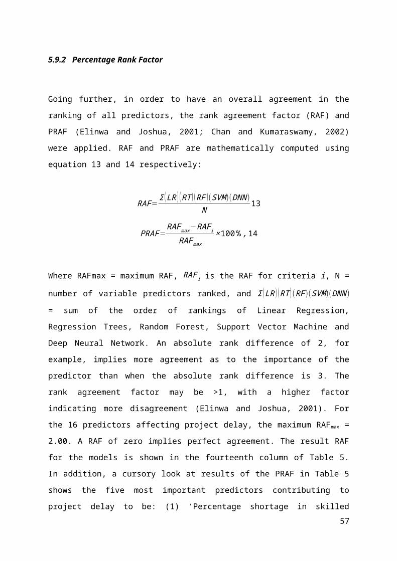
of BIM software: towards a plug-in for construction waste minimization using big data. International Journal of Sustainable Building Technology and Urban Development, 6(4), 211-228.

Bing, L., Akintoye, A., Edwards, P. J., & Hardcastle, C. (2005). The allocation of risk in PPP/PFI construction projects in the UK. International Journal of project management, 23(1), 25-35.

Boyd, D., & Crawford, K. (2012). Critical questions for big data: Provocations for a cultural, technological, and scholarly phenomenon. Information, communication & society, 15(5), 662-679.

Brown, B., Chui, M., & Manyika, J. (2011). Are you ready for the era of ‘big data’. McKinsey Quarterly, 4(1), 24-35.

Carter, G., & Smith, S. D. (2006). Safety hazard identification on construction projects. Journal of construction engineering and management, 132(2), 197-205.

Centenaro, M., Vangelista, L., Zanella, A., & Zorzi, M. (2016). Long-range communications in unlicensed bands: The rising stars in the IoT and smart city scenarios. IEEE Wireless Communications, 23(5), 60-67.

Chakrabarty, S., & Engels, D. W. (2016, January). A secure IoT architecture for Smart Cities. In Consumer Communications & Networking Conference (CCNC), 2016 13th IEEE Annual (pp. 812-813). IEEE.

Chiang, M., & Zhang, T. (2016). Fog and IoT: An overview of research opportunities. IEEE Internet of Things Journal, 3(6), 854-864.

Bossink, B.A., 2004. Managing drivers of innovation in construction networks. Journal of construction engineering and management, 130(3), pp.337-345.

Baloi, D., & Price, A. D. (2003). Modelling global risk factors affecting construction cost performance. International Journal of Project Management, 21(4), 261-269.

Burati Jr, J.L., Farrington, J.J. and Ledbetter, W.B., 1992. Causes of quality deviations in design and construction. Journal of construction engineering and management, 118(1), pp.34-49.

Ching, F.D., 2014. Building construction illustrated. John Wiley & Sons.

57

Criminisi, A., Shotton, J., & Konukoglu, E. (2012). Decision forests: A unified framework for classification, regression, density estimation, manifold learning and semi-supervised learning. Foundations and Trends® in Computer Graphics and Vision, 7(2–3), 81-227.

Davis, K., Ledbetter, W.B. and Burati Jr, J.L., 1989. Measuring design and construction quality costs. Journal of Construction Engineering and Management, 115(3), pp.385-400.

Dissanayaka, S. M., & Kumaraswamy, M. M. (1999). Evaluation of factors affecting time and cost performance in Hong Kong building projects. Engineering Construction and Architectural Management, 6(3), 287-298.

Dikmen, I., Birgonul, M.T. and Han, S., 2007. Using fuzzy risk assessment to rate cost overrun risk in international construction projects. International Journal of Project Management, 25(5), pp.494-505.

Eccles, R.G., 1981. The quasifirm in the construction industry. Journal of Economic Behavior & Organization, 2(4), pp.335-357.

Errasti, A., Beach, R., Oyarbide, A. and Santos, J., 2007. A process for developing partnerships with subcontractors in the construction industry: An empirical study. International Journal of Project Management, 25(3), pp.250-256.

El-Sayegh, S. M. (2008). Risk assessment and allocation in the UAE construction industry. International Journal of Project Management, 26(4), 431-438.

Evans, J. S., Murphy, M. A., Holden, Z. A., & Cushman, S. A. (2011). Modeling species distribution and change using random forest. In Predictive species and habitat modeling in landscape ecology (pp. 139-159). Springer New York.

Fan, J.B., Chikashige, Y., Smith, C.L., Niwa, O., Yanagida, M. and Cantor, C.R., 1989. Construction of a Not I restriction map of the fission yeast Schizosaccharomyces pombe genome. Nucleic acids research, 17(7), pp.2801-2818.

Fookes, P.G., French, W.J. and Rice, S.M.M., 1985. The influence of ground and groundwater geochemistry on construction in the Middle East.

58

Quarterly Journal of Engineering Geology and Hydrogeology, 18(2), pp.101-127.

Flyvbjerg, B., Skamris Holm, M.K. and Buhl, S.L., 2004. What causes cost overrun in transport infrastructure projects?. Transport reviews, 24(1), pp.3-18.

Fung, I. W., Tam, V. W., Lo, T. Y., & Lu, L. L. (2010). Developing a risk assessment model for construction safety. International Journal of Project Management, 28(6), 593-600.

Fight, A. (1999) Introduction to Project Finance. Oxford: Butterworth–Heinemann.

Friedman, J. H., & Stuetzle, W. (1981). Projection pursuit regression. Journal of the American statistical Association, 76(376), 817-823.

Gatzert, N., & Kosub, T. (2016). Risks and risk management of renewable energy projects: The case of onshore and offshore wind parks. Renewable and Sustainable Energy Reviews, 60, 982-998.

Gaur, A., Scotney, B., Parr, G., & McClean, S. (2015). Smart city architecture and its applications based on IoT. Procedia computer science, 52, 1089-1094.

Gransberg, D.D. and Molenaar, K., 2004. Analysis of owner's design and construction quality management approaches in design/build projects. Journal of Management in Engineering, 20(4), pp.162-169.

Hampton, G., Baldwin, A. N., & Holt, G. (2012). Project delays and cost: stakeholder perceptions of traditional v. PPP procurement. Journal of Financial Management of Property and Construction, 17(1), 73-91.

Hampton, S. E., Strasser, C. A., Tewksbury, J. J., Gram, W. K., Budden, A. E., Batcheller, A. L., ... & Porter, J. H. (2013). Big data and the future of ecology. Frontiers in Ecology and the Environment, 11(3), 156-162.

Harty, C., 2005. Innovation in construction: a sociology of technology approach. Building Research & Information, 33(6), pp.512-522.

Hopfield, J. J. (1988). Artificial neural networks. Circuits and Devices Magazine, IEEE, 4(5), 3-10.

59

Hu, H., Wen, Y., Chua, T. S., & Li, X. (2014). Toward scalable systems for big data analytics: a technology tutorial. Access, IEEE, 2, 652-687

Hendrickson, C., & Au, T. (1989). Project management for construction: Fundamental concepts for owners, engineers, architects, and builders. Chris Hendrickson.

Javed, A. A., Lam, P. T., & Chan, A. P. (2013). A model framework of output specifications for hospital PPP/PFI projects. Facilities, 31(13/14), 610-633.

Javed, A. A., Lam, P. T., & Zou, P. X. (2013). Output-based specifications for PPP projects: lessons for facilities management from Australia. Journal of Facilities Management, 11(1), 5-30.

Kaming, P. F., Olomolaiye, P. O., Holt, G. D., & Harris, F. C. (1997). Factors influencing construction time and cost overruns on high-rise projects in Indonesia. Construction Management & Economics, 15(1), 83-94.

Kazaz, A., & Ulubeyli, S. (2007). Drivers of productivity among construction workers: A study in a developing country. Building and Environment, 42(5), 2132-2140.

Kim, S. Y., Van Tuan, N., & Ogunlana, S. O. (2009). Quantifying schedule risk in construction projects using Bayesian belief networks. International Journal of Project Management, 27(1), 39-50.

KPMG Global Construction Industry Report (2015). Climbing the Curve. Online. [Accessed on 12 March, 2015] https://www.kpmg.com/Global/.../global-construction.../global-construction-survey-201.

Kittusamy, N. K., & Buchholz, B. (2004). Whole-body vibration and postural stress among operators of construction equipment: A literature review. Journal of safety research, 35(3), 255-261.

Larsen, J. K., Shen, G. Q., Lindhard, S. M., & Brunoe, T. D. (2015). Factors affecting schedule delay, cost overrun, and quality level in public construction projects. Journal of Management in Engineering, 32(1), 04015032.

60

LaValle, S., Lesser, E., Shockley, R., Hopkins, M. S., & Kruschwitz, N. (2011). Big data, analytics and the path from insights to value. MIT sloan management review, 52(2), 21.

Le-Hoai, L., Dai Lee, Y. and Lee, J.Y., 2008. Delay and cost overruns in Vietnam large construction projects: A comparison with other selected countries. KSCE journal of civil engineering, 12(6), pp.367-377.

Liaw, A., & Wiener, M. (2002). Classification and regression by randomForest. R news, 2(3), 18-2

Le-Hoai, L., Dai Lee, Y., & Lee, J. Y. (2008). Delay and cost overruns in Vietnam large construction projects: A comparison with other selected countries. KSCE journal of civil engineering, 12(6), 367-377.

Lee, J. K. (2008). Cost overrun and cause in Korean social overhead capital projects: Roads, rails, airports, and ports. Journal of Urban Planning and Development, 134(2), 59-62.

Ling, F. Y. Y., & Hoi, L. (2006). Risks faced by Singapore firms when undertaking construction projects in India. International Journal of Project Management, 24(3), 261-270

Lim, E. C., & Alum, J. (1995). Construction productivity: issues encountered by contractors in Singapore. International Journal of Project Management, 13(1), 51-58.

Li, X., Zhao, L., Wei, L., Yang, M. H., Wu, F., Zhuang, Y., ... & Wang, J. (2016). Deepsaliency: Multi-task deep neural network model for salient object detection. IEEE Transactions on Image Processing, 25(8), 3919-3930.

Love, P. E., Edwards, D. J., & Irani, Z. (2012). Moving beyond optimism bias and strategic misrepresentation: An explanation for social infrastructure project cost overruns. Engineering Management, IEEE Transactions on, 59(4), 560-571.

Lu, W., Chen, X., Ho, D. C., & Wang, H. (2016). Analysis of the construction waste management performance in Hong Kong: the public and private sectors compared using big data. Journal of Cleaner Production, 112, 521-531.

61

Lu, W., Chen, X., Peng, Y., & Shen, L. (2015). Benchmarking construction waste management performance using big data. Resources, Conservation and Recycling, 105, 49-58.

Mackenzie, S., Kilpatrick, A. R., & Akintoye, A. (2000). UK construction skills shortage response strategies and an analysis of industry perceptions. Construction Management & Economics, 18(7), 853-862.

Memos, V. A., Psannis, K. E., Ishibashi, Y., Kim, B. G., & Gupta, B. B. (2018). An efficient algorithm for media-based surveillance system (EAMSuS) in IoT smart city framework. Future Generation Computer Systems, 83, 619-628.

Mohamed, S. (2002). Safety climate in construction site environments. Journal of construction engineering and management, 128(5), 375-384.

Mezher, T. M., & Tawil, W. (1998). Causes of delays in the construction industry in Lebanon. Engineering, Construction and Architectural Management, 5(3), 252-260.

Moselhi, O., Gong, D. and El-Rayes, K., 1997. Estimating weather impact on the duration of construction activities. Canadian Journal of Civil Engineering, 24(3), pp.359-366.

Mustafa, M.A. and Al-Bahar, J.F., 1991. Project risk assessment using the analytic hierarchy process. Engineering Management, IEEE Transactions on, 38(1), pp.46-52.

Mohamed, S. (2002). Safety climate in construction site environments. Journal of construction engineering and management, 128(5), 375-384.

Ng, A., & Loosemore, M. (2007). Risk allocation in the private provision of public infrastructure. International Journal of Project Management, 25(1), 66-76.

Newey, W. K., & West, K. D. (1994). Automatic lag selection in covariance matrix estimation. The Review of Economic Studies, 61(4), 631-653.

Ohlhorst, F. J. (2012). Big data analytics: turning big data into big money. John Wiley & Sons.

62

Odeh, A.M. and Battaineh, H.T., 2002. Causes of construction delay: traditional contracts. International journal of project management, 20(1), pp.67-73.

Pal, R., Wang, P., & Liang, X. (2017). The critical factors in managing relationships in international engineering, procurement, and construction (IEPC) projects of Chinese organizations. International Journal of Project Management, 35(7), 1225-1237.

Pal, M. (2005). Random forest classifier for remote sensing classification. International Journal of Remote Sensing, 26(1), 217-222.

Palomo, J., Rios Insua, D., & Ruggeri, F. (2007). Modeling external risks in project management. Risk analysis, 27(4), 961-978.

Rathore, M. M., Ahmad, A., Paul, A., & Rho, S. (2016). Urban planning and building smart cities based on the internet of things using big data analytics. Computer Networks, 101, 63-80.

Rebeiz, K. S. (2011). Public–private partnership risk factors in emerging countries: BOOT illustrative case study. Journal of Management in Engineering, 28(4), 421-428.

Robinson, H. S., & Scott, J. (2009). Service delivery and performance monitoring in PFI/PPP projects. Construction Management and Economics, 27(2), 181-197.

Rousseau, D. M., & Libuser, C. (1997). Contingent workers in high risk environments. California Management Review, 39(2), 103-123.

Rodriguez-Galiano, V. F., Ghimire, B., Rogan, J., Chica-Olmo, M., & Rigol-Sanchez, J. P. (2012). An assessment of the effectiveness of a random forest classifier for land-cover classification. ISPRS Journal of Photogrammetry and Remote Sensing, 67, 93-104.

Russell, J. S., & Jaselskis, E. J. (1992). Predicting construction contractor failure prior to contract award. Journal of construction engineering and management, 118(4), 791-811.

Sawacha, E., Naoum, S., & Fong, D. (1999). Factors affecting safety performance on construction sites. International journal of project management, 17(5), 309-315.

63

Sagiroglu, S., & Sinanc, D. (2013, May). Big data: A review. In Collaboration Technologies and Systems (CTS), 2013 International Conference on (pp. 42-47). IEEE.

Scuotto, V., Ferraris, A., & Bresciani, S. (2016). Internet of Things: Applications and challenges in smart cities: a case study of IBM smart city projects. Business Process Management Journal, 22(2), 357-367.

Silver, D., Huang, A., Maddison, C. J., Guez, A., Sifre, L., Van Den Driessche, G., ... & Dieleman, S. (2016). Mastering the game of Go with deep neural networks and tree search. nature, 529(7587), 484.

Shane, J. S., Molenaar, K. R., Anderson, S., & Schexnayder, C. (2009). Construction project cost escalation factors. Journal of Management in Engineering, 25(4), 221-229.

Sanger, F.J. and Sayles, F.H., 1979. Thermal and rheological computations for artificially frozen ground construction. Engineering geology, 13(1), pp.311-337.

Semple, C., Hartman, F.T. and Jergeas, G., 1994. Construction claims and disputes: causes and cost/time overruns. Journal of construction engineering and management, 120(4), pp.785-795.

Shen, L. Y., Li Hao, J., Tam, V. W. Y., & Yao, H. (2007). A checklist for assessing sustainability performance of construction projects. Journal of civil engineering and management, 13(4), 273-281.

Sun, M. and Meng, X., 2009. Taxonomy for change causes and effects in construction projects. International Journal of Project Management, 27(6), pp.560-572.

Svetnik, V., Liaw, A., Tong, C., Culberson, J. C., Sheridan, R. P., & Feuston, B. P. (2003). Random forest: a classification and regression tool for compound classification and QSAR modeling. Journal of chemical information and computer sciences, 43(6), 1947-1958.

Tatum, C.B., 1987. Process of innovation in construction firm. Journal of Construction Engineering and Management, 113(4), pp.648-663.

64

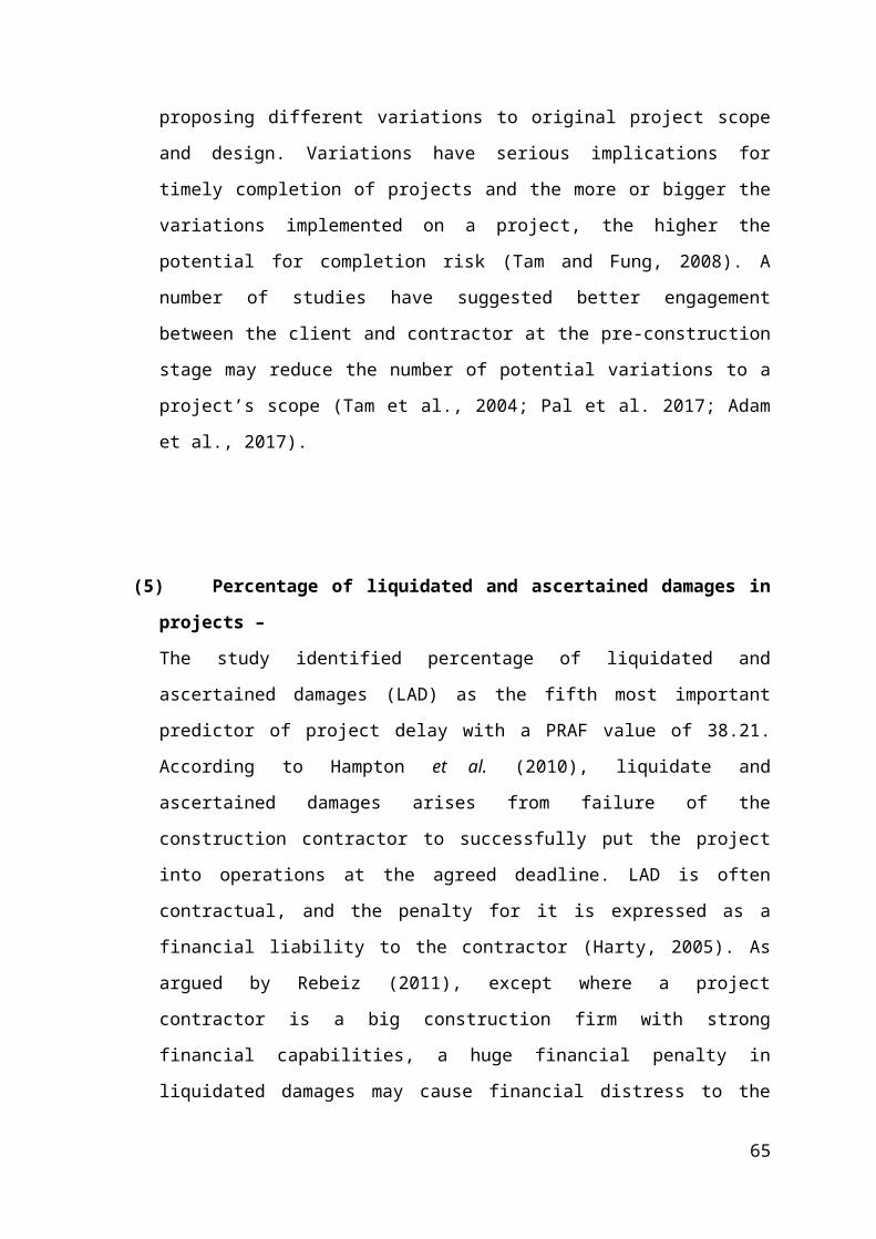
Tatum, C.B., 1989. Organizing to increase innovation in construction firms. Journal of Construction Engineering and Management, 115(4), pp.602-617.

Tolman, F.P., 1999. Product modeling standards for the building and construction industry: past, present and future. Automation in construction, 8(3), pp.227-235.

Talia, D. (2013). Toward Cloud-based Big-data Analytics. IEEE Computer Science, 98-101.

Tam, C. M., Zeng, S. X., & Deng, Z. M. (2004). Identifying elements of poor construction safety management in China. Safety Science, 42(7), 569-586

Tam, V. W. Y., & Fung, I. W. H. (2008). A study of knowledge, awareness, practice and recommendations among Hong Kong construction workers on using personal respiratory protective equipment at risk. Open Construction and Building Technology Journal, 2, 69-81.

Tam, C. M., Zeng, S. X., & Deng, Z. M. (2004). Identifying elements of poor construction safety management in China. Safety Science, 42(7), 569-586.

Teizer, J., Allread, B. S., Fullerton, C. E., & Hinze, J. (2010). Autonomous pro-active real-time construction worker and equipment operator proximity safety alert system. Automation in Construction, 19(5), 630-640.

Theobald, C. M. (1974). Generalizations of mean square error applied to ridge regression. Journal of the Royal Statistical Society. Series B (Methodological), 103-106.

Teo, E. A. L., Ling, F. Y. Y., & Chong, A. F. W. (2005). Framework for project managers to manage construction safety. International Journal of project management, 23(4), 329-341.

Tiong, R. L. (1990). BOT projects: risks and securities. Construction Management and Economics, 8(3), 315-328.

Toole, T. M. (2002). Construction site safety roles. Journal of Construction Engineering and Management, 128(3), 203-210.

65

Tibshirani, R. (1996). Regression shrinkage and selection via the lasso. Journal of the Royal Statistical Society. Series B (Methodological), 267-288.

True, W.R., 1998. Weather, construction inflation could squeeze North American pipelines. Oil and Gas Journal, 96(35).

Van Staveren, M.T., 2006. Uncertainty and ground conditions. A risk management approach.

Van, L. T., Sang, N. M., & Viet, N. T. (2015). A conceptual model of delay factors affecting government construction projects. ARPN Journal of Science and Technology, 5(2), 92-100.

Wu, X., Zhu, X., Wu, G. Q., & Ding, W. (2014). Data mining with big data. Knowledge and Data Engineering, IEEE Transactions on, 26(1), 97-107.

Wu, J., Guo, S., Li, J., & Zeng, D. (2016). Big data meet green challenges: big data toward green applications. IEEE Systems Journal, 10(3), 888-900.

W.M. Chan and M. Kumaraswamy, (2002). Compressing construction durations: Lessons learned from Hong Kong building projects, Int. J. Proj. Manag. 20(1), pp. 23–35.

doi:10.1016/S0263-7863(00)00032-6.

Yang, J.B. and Wei, P.R., 2010. Causes of delay in the planning and design phases for construction projects. Journal of Architectural Engineering, 16(2), pp.80-83.

Zou, P. X., Zhang, G., & Wang, J. (2007). Understanding the key risks in construction projects in China. International Journal of Project Management, 25(6), 601-614.

Zwikael, O., & Ahn, M. (2011). The effectiveness of risk management: an analysis of project risk planning across industries and countries. Risk analysis, 31(1), 25-37.

66