B4 Estimation and Inference

6 Lectures Hilary Term 2007

2 Tutorial Sheets A. Zisserman

Overview

• Lectures 1 & 2: Introduction – sensors, and basics of probability density functions for representing sensor error and uncertainty.

• Lecture 3 & 4: Estimators – Maximum Likelihood (ML) and Maximum a Posteriori (MAP).

• Lecture 5 & 6: Decisions and classification – loss functions, discriminant functions, linear classifiers.

Textbooks 1

• Estimation with Applications to Tracking and Navigation: Theory Algorithms and SoftwareYaakov Bar-Shalom, Xiao-Rong Li, Thiagalingam Kirubarajan, Wiley, 2001

Covers probability and estimation, but contains much more material than required for this course. Use also for C4B Mobile Robots.

Textbooks 2

• Pattern ClassificationRichard O. Duda, Peter E. Hart, David G. Stork, Wiley, 2000

Covers classification, but also contains much more material than required for this course.

Background reading and web resources

• Information Theory, Inference, and Learning Algorithms.

David J. C. MacKay, CUP, 2003• Covers all the course material though at an advanced level

• Available on line

• Introduction to Random Signals and Applied KalmanFiltering.

R. Brown and P. Hwang, Wiley, 1997

• Good review of probability and random variables in first chapter

• Further reading (www addresses) and the lecture notes are on http://www.robots.ox.ac.uk/~az/lectures

One more book for background reading …

• Pattern Recognition and Machine Learning

Christopher Bishop, Springer, 2006.

• Excellent on classification and regression

• Quite advanced

Introduction: Sensors and estimation

Sensors are used to give information about the state of some system.

Our aim in this course is to develop methods which can be used to combine multiple sensor measurements

• possibly from multiple sensors

• possibly over time

with prior information to obtain accurate estimates of a system’s state

Noise and uncertainty in sensors

• Real sensors give inexact measurements for a variety of reasons:

• discretization error (e.g. measurements on a grid)

• calibration error

• quantization noise (e.g. CCD)

• …

• Successive observations of a system or phenomena do not produceexactly the same result

• Statistical methods are used to describe and understand this variability, and to incorporate variability into the decision-making processes

• Examples: ultrasound, laser range scanner, CCD images, GPS

Ultrasound – objective: diagnose heart disease

Contrast agent enhanced Doppler velocity image

Axial view

Brightness codes depth

• use prior “shape model” for heart for inference

Laser range scanner – objective: build map of room

• Good quality data up to discretization on a grid

y

x

CCD sensor – objective: read number plate

• 100 frame low light sequence

•Temporal average to suppress mean zero additive noiseI(t) = I + n(t)

0 frames5 frames10 frames20 frames40 frames80 frames100 frames

• Average N noise samples with zero mean and variance result has zero mean and variance /N

Time averaged frames

histogram equalized

GPS – objective: estimate car trajectory

1000 1050 1100 1150

-2700

-2680

-2660

-2640

-2620

-2600

GPS data collected from car

Global Positioning System

close-up

1072 1072.5 1073 1073.5 1074 1074.5 1075 1075.5 1076 1076.5

-2635.5

-2635

-2634.5

-2634

-2633.5

-2633

-2632.5

-2632

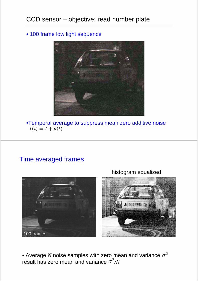
GPS: error sources

• fit (estimate) curve and lines to reduce random errors

1. Regression

• estimate parameters, e.g. of line fit to trajectory of car

2. Classification

• estimate class, e.g. handwritten digit classification

Two canonical estimation problems

1

7

?

?

The need for probability

We have seen that there is uncertainty in the measurements due to sensor noise.

There may also be uncertainty in the model we fit.

Finally, we often want more than just a single value for an estimate, we would also like to model the confidence or uncertainty of the estimate.

Probability theory – the “calculus of uncertainty” – provides the mathematical machinery.

Revision of Probability Theory

• probability distribution functions (pdf)

• joint and conditional probability

• independence

• Normal (Gaussian) distributions of one and two variables

1D Probability – a brief review

Discrete sets

Suppose an experiment has a set of possible outcomes S, and an “event” E is a sub-set of S, then

probability of E = relative frequency of event

=number of outcomes in E

total number of outcomes in S

e.g. throw a die, then probability of any particular number = 1/6; and probability of an even number = 1/2

If S = {a1, a2, . . . , an} has probabilities {p1, p2, . . . , pn} then

pi ≥ 0nXi=1

pi = 1

Probability density function (pdf)

p(x)

x x+dxprobability over a range of x is given by area under the curve

P(x < X < x+ dx) = p(x) dx

Z ∞−∞

p(x)dx = 1

PDF Example 1 – Univariate Normal Distribution

The most important example of a continuous density/distribution is the normal or Gaussian distribution.

-6 -4 -2 0 2 4 60

0.05

0.1

0.15

0.2

0.25

0.3

0.35

0.4

µ = 0 σ = 1

e.g. model sensor response for measured x, when true x = 0

p(x) =1√2πσ

exp(−(x− µ)2

2σ2) x ∼ N(µ,σ2)

PDF Example 2 – A Uniform Distribution

p(x) ∼ U(a, b)

a b

1b−a

• example: laser range finder

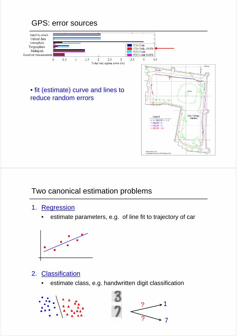
PDF Example 3 – A histogram

• image intensity histogram

frequency

intensity• normalize to obtain a pdf

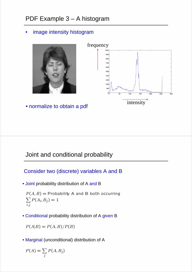
Joint and conditional probability

Consider two (discrete) variables A and B

• Joint probability distribution of A and B

• Conditional probability distribution of A given B

• Marginal (unconditional) distribution of A

P(A,B) = Probability A and B both occurringXi,j

P(Ai,Bj) = 1

P(A|B) = P(A,B)/P(B)

P(A) =Xj

P(A,Bj)

Example

Consider two sensors measuring the x and y coordinates of an object in 2D

The joint distribution is given by the “spreadsheet”,

where the array entry (i, j) is P (X = i, Y = j):

X = 0 X = 1 X = 2 row sum

Y = 0 0.32 0.03 0.01 0.36Y = 1 0.06 0.24 0.02 0.32Y = 2 0.02 0.03 0.27 0.32

To compute the joint distribution

1. Count the number of times the measured

location is at (X,Y) for X=0,2; Y=0,2

2. Normalize the count matrix such that Xi,j

P(i, j) = 1 X

Y

Exercise: Compute the marginals and conditional P( Y | X=1 )

marginal

X = 0 X = 1 X = 2 row sumY = 0 0.32 0.03 0.01 0.36Y = 1 0.06 0.24 0.02 0.32Y = 2 0.02 0.03 0.27 0.32

col sum 0.40 0.30 0.30 1.0

marginal P(Y=0)

P (X = 1) =XY

P(X = 1, Y )

Conditional P( Y | X=1 )

• normalize P(X=1,Y) so that it is a probability

• in words “the probability of Y given that X = 1”

X = 1Y = 0 0.03 / 0.30Y = 1 0.24 / 0.30Y = 2 0.03 / 0.30

col sum 1.00P(Y |X = 1) = P(X = 1, Y )

P(X = 1)

Bayes’ Rule (or Bayes’ Theorem)

From the definition of the conditional

Hence

• lets the dependence of the conditionals be reversed

• will be important later for Maximum a Posteriori (MAP) estimation

Writing

P(A|B) = P(B|A)P(A)P (B)

P (B) =Xi

P(Ai, B) =Xi

P (B|Ai)P(Ai)

P(A|B) = P(B|A)P(A)P (B)

=P (B|A)P (A)Pi P(B|Ai)P (Ai)

P (A,B) = P(A|B)P (B)P (A,B) = P(B|A)P (A)

Bayes’ Rule

with similar expressions for P(B|A)

Independent variables

Two variables are independent if (and only if)

p(A,B) = p(A)p(B)

Compare with conditional probability

So and similarly

e.g.

• two throws of a dice or coin are independent

• two cards picked without replacement from the same pack are not independent

p(A,B) = p(A|B)p(B)

i.e. all joint values = product of the marginals

p(A|B) = p(A) p(B|A) = p(B)

× 0.5 0.5

H1 T1 row sumH2 0.25 0.25 0.50T2 0.25 0.25 0.50

col sum 0.50 0.50 1.0

=0.50.5

X = 0 X = 1 X = 2 row sumY = 0 0.32 0.03 0.01 0.36Y = 1 0.06 0.24 0.02 0.32Y = 2 0.02 0.03 0.27 0.32

col sum 0.40 0.30 0.30 1.0

X = 0 X = 1 X = 2 row sumY = 0 0.09 0.12 0.09 0.30Y = 1 0.12 0.16 0.12 0.40Y = 2 0.09 0.12 0.09 0.30

col sum 0.30 0.40 0.30 1.0

Examples

• are these joint distributions independent?

y

x

y

x

y

x

Joint, conditional and independence for pdfs

Similar results apply for pdfs of continuous variables x and y

xy

probability over a range of x and y is given by volume

Z ∞−∞

Z ∞−∞

p(x, y)dxdy = 1

Bivariate normal distribution

mean covariance

x=

Ãxy

!µ =

õxµy

!Σ=

"Σ11 Σ12Σ21 Σ22

#

N (x|µ,Σ) = 1

2π |Σ|1/2exp

½−12(x− µ)>Σ−1(x− µ)

¾

Example

p(x, y) =1

2πσxσyexp

(−12

Ãx2

σ2x+y2

σ2y

!)µ=

Ã00

!Σ=

"σ2x 0

0 σ2y

#=

"4 00 1

#

Note

• iso-probability contour curves are ellipses

• p(x,y) = p(x)p(y) so x is independent of y

-5 -4 -3 -2 -1 0 1 2 3 4 5-5

-4

-3

-2

-1

0

1

2

3

4

5

x2

σ2x+y2

σ2y= d2

Conditional distribution

i.e. independent

p(x|y) = p(x, y)

p(y)=

12πσxσy

exp

½−12

µx2

σ2x+ y2

σ2y

¶¾1√2πσy

exp

½− y2

2σ2y

¾

=1√2πσx

exp

(− x2

2σ2x

)

N (x|µ,Σ) = 1

(2π)n/2 |Σ|1/2exp

½−12(x− µ)>Σ−1(x− µ)

¾Normal distribution of n variables

where

• x is a n-component column vector

• is the n-component mean vector

• is a n x n covariance matrix

µ

Σ

Lecture 2: Describing and manipulating pdfs

• Expectations of moments in 1D• Mean, variance, skew, kurtosis

• Expectations of moments in 2D• Covariance and correlation

• Transforming variables

• Combining pdfs

• Introduction to Maximum Likelihood estimation

Describing distributions

-4 -2 0 2 4 6 8 10 120

20

40

60

80

100

120

140

160

1D 2D

• could store original measurements (xi, yi) , or

• store histogram of measurements pi, or

• compute (fit) a compact representation of the distribution

Repeated measurements with the same sensor

Sensor model:

Discrete case

Continuous case

Note that E is a linear operator, i.e.

Expectations and moments – 1D

The expected value of a scalar random variable, also called its mean, average, or first moment is:

E[x] =nXi=1

pixi

E[ax+ by] = aE[x] + bE[y]

E[x] =Z ∞−∞

xp(x) dx = µ

The square root of the variance is the standard deviation

Moments

The nth moment is

E[xn] =Z ∞−∞

xnp(x) dx

The second central moment, or variance, is

var(x) = E[(x−µ)2] =Z ∞−∞(x−µ)2p(x) dx = E[x2]−µ2 = σ2x

σ

-4 -2 0 2 4 6 8 10 120

0

0

0

0

0

0

0

0

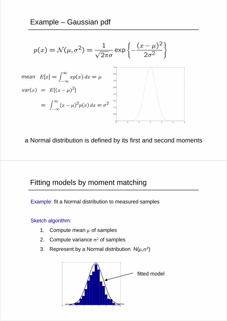
Example – Gaussian pdf

-6 -4 -2 0 2 4 60

0.05

0.1

0.15

0.2

0.25

0.3

0.35

0.4

a Normal distribution is defined by its first and second moments

mean E[x] =Z ∞−∞

xp(x) dx= µ

var(x) = E[(x− µ)2]

=

Z ∞−∞(x − µ)2p(x) dx = σ2

p(x) = N(µ,σ2) = 1√2πσ

exp

(−(x− µ)

2

2σ2

)

Fitting models by moment matching

Example: fit a Normal distribution to measured samples

Sketch algorithm:

1. Compute mean µ of samples

2. Compute variance σ2 of samples

3. Represent by a Normal distribution N(µ,σ2)

-4 -2 0 2 4 6 8 10 120

0

0

0

0

0

0

0

0

fitted model

Mean and Variance of discrete random variable

• two probability distributions can differ even though they have identical means and variance

• mean and variance are summary values; more is needed to know the distribution (e.g. that it is a normal distribution)

What model should be fitted to this measured distribution ?

• what does the fitted Normal distribution look like ?

Higher moments - skewness

-6 -4 -2 0 2 4 60

0.05

0.1

0.15

0.2

0.25

0.3

0.35

0.4

skew(x) = E[

Ãx − µµ

!3] =

Z ∞−∞

Ãx− µµ

!3p(x) dx

symmetric (e.g. Gaussian): skew = 0 skew positive

Higher moments - kurtosis

Gaussian): kurt = 0

positive: narrow peak with long tails

negative: flat peak and little tail

kurt(x) = E[µx − µσ

¶4]−3 =

Z ∞−∞

µx− µσ

¶4p(x) dx−3

Suppose we have 2 random variables with bivariate joint density:

Define moments (expectation of their product)

Expectations and moments – 2D

xy

p(x, y)

x

y

E[xy] =Zxyp(x, y) dxdy

= E[x]E[y] if x and y are independent

NB not if and only if

Covariance and Correlation

• measure behaviour about mean

• the covariance is defined as

• summarize as a 2 x 2 symmetric covariance matrix

• in n dimensions covariance is a n x n symmetric matrix

cov(xy) = σxy =Z(x − µx)(y − µy)p(x, y) dxdy

= E[xy]− E[x]E[y] [proof: exercise]

Σ =

"var(x) cov(xy)cov(xy) var(y)

#= E

h(x− µ)(x− µ)>

i

• the correlation is defined as

• measures normalized correlation of two random variables (c.f. correlation of two signals)

• in the discrete sample case

• | ρ(xy) | · 1

• e.g. if x = y then ρ(x,y) = 1, if x = -y then ρ(x,y) = -1

• if x and y are independent then ρ(x,y) = cov(x,y) = 0

ρ(xy) =cov(xy)q

var(x)qvar(y)

ρ(xy) =

Pi(xi− µx)(yi− µy)qP

i(xi− µx)2qP

i(yi− µy)2

Fitting a Bivariate Normal distribution

xy

x

y

N (x|µ,Σ) = 1

2π |Σ|1/2exp

½−12(x− µ)>Σ−1(x− µ)

¾

• a Normal distribution in 2D is defined by its first and second moments (mean and covariance matrix)

• in a similar manner to the 1D case, a 2D Gaussian is fitted by computing the mean and covariance matrix of the samples

Example

-6 -4 -2 0 2 4 6-5

-4

-3

-2

-1

0

1

2

3

4

5

• if x and y are not independent and have correlation ρ,

Σ =

"σ2x ρσxσy

ρσxσy σ2y

#

Let S = Σ−1 then iso-probability curves are x>Sx= d2, i.e. ellipses

µ=

Ã00

!Σ =

"4 1.21.2 1

#

Transformation of random variables

Problem: Suppose the pdf for a dart thrower is

express this pdf in polar coordinates.

• The coordinates are related as

• and taking account of the area change

x = x(r, θ) = r cos θ

y = y(r, θ) = r sinθ

p(x, y)dxdy = p(x(r, θ), y(r, θ))J drdθ

p(x, y) =1

2πσ2e−(x

2+y2)/(2σ2)

where J is the Jacobian, and J = r in this case

p(x(r, θ), y(r, θ))J drdθ =1

2πσ2e−r

2/(2σ2)r drdθ

prθ(r, θ)

p(r) =Z 2π0

p(r, θ) dθ =r

2πσ2e−r

2/(2σ2)Z 2π0

dθ

=r

σ2e−r

2/(2σ2)

marginalize to get p(r)

0 1 2 3 4 5 60

0.05

0.1

0.15

0.2

0.25

r

p(r)

σ

Example 1: Linear transformation of Normal distributions

p(x) = N (µ,Σ) = 1

(2π)n/2 |Σ|1/2exp

½−12(x− µ)>Σ−1(x− µ)

¾If the pdf of x is a Normal distribution

then under the linear transformation

the pdf of y is also a Normal distribution with

y = Ax+ t

µy = Aµx+ t

Σy = AΣxA>

Consider the quadratic term

Under the transformation

y = Ax+ t → x = A−1(y− t)developing the quadratic

(x− µx)>Σ−1x (x− µx)

= (A−1(y− t)− µx)>Σ−1x (A−1(y− t)− µx)=

³A−1(y− t−Aµx)

´>Σ−1x

³A−1(y − t−Aµx)

´= (y− t− Aµx)>A−>Σ−1x A−1 (y− t−Aµx)= (y− µy)>Σ−1y (y− µy)with

µy = Aµx+ t

Σ−1y = A−>Σ−1x A−1 → Σy = AΣxA>

Example 2: Sum of random variables

Problem: suppose z = x + y and pxy(x,y) is the joint distribution of x and y, find p(z)

x

y

z z+dz

t

Let t= x − y then

p(z) =Z ∞−∞

ptz(t, z) dt

=Z ∞−∞1

2pxy(

z+ t

2,z − t2) dt

=Z ∞−∞

pxy(z − u, u) du where u=z − t2

=Z ∞−∞

px(z − u)py(u) du if x and y independent

ptz(t, z) dtdz = pxy(x, y)J dtdz

=1

2pxy(

z + t

2,z − t2) dtdz

which is the convolution of px(x) and py(y)

-6 -4 -2 0 2 4 6-0.5

0

0.5

1

1.5

2

2.5

3

-6 -4 -2 0 2 4 60

0.1

0.2

0.3

0.4

0.5

0.6

0.7

0.8

Example: 1D Gaussians

Add the means and covariances

[proof: exercise]

p(x) = N(µx,σ2x) p(y) = N(µy,σ

2y )

then

p(x+ y) = N(µx, σ2x) ∗ N(µy, σ2y )

= N(µx+ µy, σ2x + σ2y)

p(x) = N(µx,σ2x) p(y) = N(µy,σ

2y )

then

p(x+ y) = N(µx, σ2x) ∗ N(µy, σ2y )

= N(µx+ µy, σ2x + σ2y)

p(x) = N(µx,σ2x) p(y) = N(µy,σ

2y )

then

p(x+ y) = N(µx, σ2x) ∗ N(µy, σ2y )

= N(µx+ µy, σ2x + σ2y)

Maximum Likelihood Estimation – informal

Estimation is the process by which we infer the value of a quantity of interest, θ, by processing data z that is some way dependent on θ.

Simple example: fitting a line to measured data

Estimate line parameters θ=(a,b), given measurements zi = (xi, yi) and model of the sensor noise

y = ax + by

x

mina,b

nXi

(yi− (axi+ b))2Least squares solution

Consider a generative model for the data

• no noise on xi

• on y:

yi = yi +ni ni ∼ N(0, σ2)

measured value

true value

p(yi|yi) ∼ e−(yi−yi)

2

2σ2

Model to be estimated yi = axi + b

p(yi|axi + b) ∼ e−(yi−(axi+b))2

2σ2

probability of measuring given that true value is yi

yi

For n points, assuming independence

measureddata

parameters

this is the likelihood

p(y1, y2, . . . yn|x1, x2, . . . xn;a, b) ∼nYi

e−(yi−(axi+b))

2

2σ2

p(y|a, b) ∼nYi

e−(yi−(axi+b))

2

2σ2

The Maximum likelihood (ML) estimate is obtained as

{a, b}= argmaxa,b

p(y|a, b)

Take negative log

The Maximum likelihood (ML) estimate is equivalent to

p(y|a, b) ∼nYi

e−(yi−(axi+b))

2

2σ2 = e−Pn

i(yi−(axi+b))2

2σ2

− log(p(y|a, b)) ∼nXi

(yi− (axi+ b))2

2σ2

{a, b} = argmina,b

nXi

(yi − (axi+ b))2

2σ2

i.e. to least squares