Autotuning of a PID-controller - Automatic · PDF fileAutotuning of a PID-controller. (Autom atisk inställning av PID-regulatorer) Abstract This master´s thesis has been performed

ISSN 0280-5316 ISRN LUTFD2/TFRT--5728--SE

Autotuning of a PID-controller

Camilla Andersson Mirjam Lindberg

Department of Automatic Control Lund Institute of Technology

October 2004

Document name MASTER THESIS Date of issue October 2004

Department of Automatic Control Lund Institute of Technology Box 118 SE-221 00 Lund Sweden Document Number

ISRNLUTFD2/TFRT--5728--SE Supervisor Mattias Grundelius TAC, Malmö Tore Hägglund LTH, Lund

Author(s) Camilla Andersson and Mirjam Lindberg

Sponsoring organization

Title and subtitle Autotuning of a PID-controller. (Automatisk inställning av PID-regulatorer)

Abstract This master´s thesis has been performed in cooperation with TAC in Malmö. The TAC group makes commercial buildings smarter by integrating and automating the technical systems required to run them. TAC:s control systems use PID-controllers to control processes such as heating and ventilation. The PID-controllers are often badly tuned, since it is too timeconsuming to calculate good PID-parameters at the time of deployment. A simple way of finding PID-parameters that give faster control loops is needed. To solve this problem the thesis proposes an autotuner based on the areamethod Method of Moments and the AMIGO tuning rules. The implementation of the autotuner using IEC 61131 is described. The resulting autotuner is tested on simulated processes and gives satisfactory results. The thesis also includes practical insights on the use of the autotuner.

Keywords

Classification system and/or index terms (if any)

Supplementary bibliographical information ISSN and key title 0280-5316

ISBN

Language English

Number of pages 38

Security classification

Recipient’s notes

The report may be ordered from the Department of Automatic Control or borrowed through: University Library Box 3, SE-221 00 Lund, Sweden. Fax +46 46 222 42 43

Contents

1 Introduction 3

1.1 About TAC . . . . . . . . . . . . . . . . . . . . . . . . . . . . 31.2 Background . . . . . . . . . . . . . . . . . . . . . . . . . . . . 3

1.2.1 The Concept of Autotuning . . . . . . . . . . . . . . . 31.2.2 Autotuning at TAC . . . . . . . . . . . . . . . . . . . 4

2 Methods 6

2.1 A Step Response Method . . . . . . . . . . . . . . . . . . . . 62.1.1 Process Identi�cation: the Three-Parameter Model . . 62.1.2 Design Method . . . . . . . . . . . . . . . . . . . . . . 92.1.3 The Method of Moments in Practice . . . . . . . . . . 9

2.2 The Relay Feedback Method . . . . . . . . . . . . . . . . . . . 112.2.1 Process Identi�cation . . . . . . . . . . . . . . . . . . . 112.2.2 Design Method . . . . . . . . . . . . . . . . . . . . . . 122.2.3 The Relay Feedback Method in Practice . . . . . . . . 13

2.3 Discussion . . . . . . . . . . . . . . . . . . . . . . . . . . . . . 13

3 Implementation 15

3.1 IEC 61131 and PLC programming in CoDeSys . . . . . . . . 153.2 Overview of the Implementation . . . . . . . . . . . . . . . . 163.3 Detailed Implementation . . . . . . . . . . . . . . . . . . . . . 17

3.3.1 Initial Phase . . . . . . . . . . . . . . . . . . . . . . . 173.3.2 Closed Loop Phase . . . . . . . . . . . . . . . . . . . . 183.3.3 Open Loop Phase . . . . . . . . . . . . . . . . . . . . . 203.3.4 PID-design Phase . . . . . . . . . . . . . . . . . . . . . 203.3.5 Disturbance Detection . . . . . . . . . . . . . . . . . . 203.3.6 Filtering . . . . . . . . . . . . . . . . . . . . . . . . . . 23

4 Test Results 24

4.1 Lag Dominated Process . . . . . . . . . . . . . . . . . . . . . 244.2 Delay Dominated Process . . . . . . . . . . . . . . . . . . . . 264.3 Balanced Process . . . . . . . . . . . . . . . . . . . . . . . . . 274.4 Process with Noise and Dead Zone . . . . . . . . . . . . . . . 28

1

CONTENTS 2

4.5 Testing on an Air Handling Unit . . . . . . . . . . . . . . . . 30

5 Conclusions 31

5.1 Summary . . . . . . . . . . . . . . . . . . . . . . . . . . . . . 315.2 User Notes . . . . . . . . . . . . . . . . . . . . . . . . . . . . . 315.3 Future Work . . . . . . . . . . . . . . . . . . . . . . . . . . . 32

A Figures 34

A.1 FBD � Overview of the Communication Parameters . . . . . 34A.2 SFC � Overview of the Autotuner Algorithm . . . . . . . . . 35

Chapter 1

Introduction

1.1 About TAC

TAC designs and manufactures systems for Building IT. This covers func-tions such as access control, heating and cooling, ventilation and lighting.With TACs integrated systems, functions such as these can be controlledand monitored from a computer terminal.

Heating, cooling and ventilation functions include controlling entities suchas temperature and air�ow. This means using feedback control loops.

A typical TAC product is the Xenta R© 300. It is a programmable controllerwith functionality including control loops, alarm handling and time control.The minimum sample time is 1 second. When control loops are implemented,di�erent PID-controllers may be used. The autotuner is tested with thePIDP-block, which uses a discrete time positional PID algorithm. The PIDP-block has dead zone capability which means that when the control error issmaller than the dead zone the controller output remains unchanged. Thesize of the dead zone is related to the accuracy of the measuring instrument.

1.2 Background

1.2.1 The Concept of Autotuning

An autotuner is a device that automatically computes the parameters of acontroller. The goal is to achieve the best control possible given the tuningobjectives. The goal is not to replace a human control engineer. The auto-tuner should rather be seen as an aid to improvement. Many PID-controllersin the �eld use the default parameter settings, since it is too time-consuming

3

CHAPTER 1. INTRODUCTION 4

to tune them manually and the systems seem to work anyway. However,badly tuned controllers cannot only lead to less e�cient control loops, theycan also lead to unpredictable system behavior when control loops are hier-archically dependent. An autotuner can be of great help in spotting thesekinds of problems as well as remedying them [1].

It is important to distinguish between autotuning and adaptive control. Anautotuning operation is run on the user's initiative, and takes place duringa limited time. When autotuning has been performed the control loop re-sumes normal operation with the new parameters. An adaptive controllercontinually changes its parameters during operation.

An autotuner follows the same approach that a control engineer would whentuning a controller:

1. Process Model � Choose a model for the process

2. Process Identi�cation � Collect process data and �t it to the model

3. Design Method � Compute the new parameters

The tuning objectives of the autotuner are process speci�c and must bedetermined before implementation. Some objectives could be low overshoot,fast setpoint tracking and good disturbance rejection. Sometimes trade-o�smust be made. Another important feature of an autotuner is usability. Ifthe autotuner is di�cult to use, it will probably not be used. The autotunershould not require a lot of user input to achieve good tuning. In the idealcase a start button should be enough.

1.2.2 Autotuning at TAC

Most of TACs control systems use PID-controllers. It is important that thePID-parameters are correctly tuned to achieve the high energy conservationmade possible by TACs integrated systems. Today not much time is spent�netuning the controllers when a system is deployed. Usually "safe" param-eters will be set which ensure that the system is stable. These parametersmostly result in slow and ine�cient control. Calculating e�cient parametersmanually is too timeconsuming. An autotuner will make the deploymentprocess run smoother and give TACs customers better results.

Autotuning has been used at TAC before. It was implemented in the early90's and based on a patented method developed at the Dept. of Auto-matic Control, Lund Institute of Technology. Together with the autotunera controller was implemented with an algorithm di�erent from the standardPID-algorithm. This autotuner does not only give the controller parametersbut also a recommended sample interval based on the process dynamic.

CHAPTER 1. INTRODUCTION 5

The new autotuner di�ers from the old autotuner since it is detached andcommunicates with the controller through a network. The basic idea isthat the new autotuner will be able to communicate with any of the todayexisting PID-controllers at TAC. It is also di�erent in the way it identi�esthe unknown process.

Chapter 2

Methods

In this chapter two di�erent process identi�cation methods with correspond-ing design methods are described. Based on MATLAB testing, one of themethods is chosen for the autotuner.

2.1 A Step Response Method

2.1.1 Process Identi�cation: the Three-Parameter Model

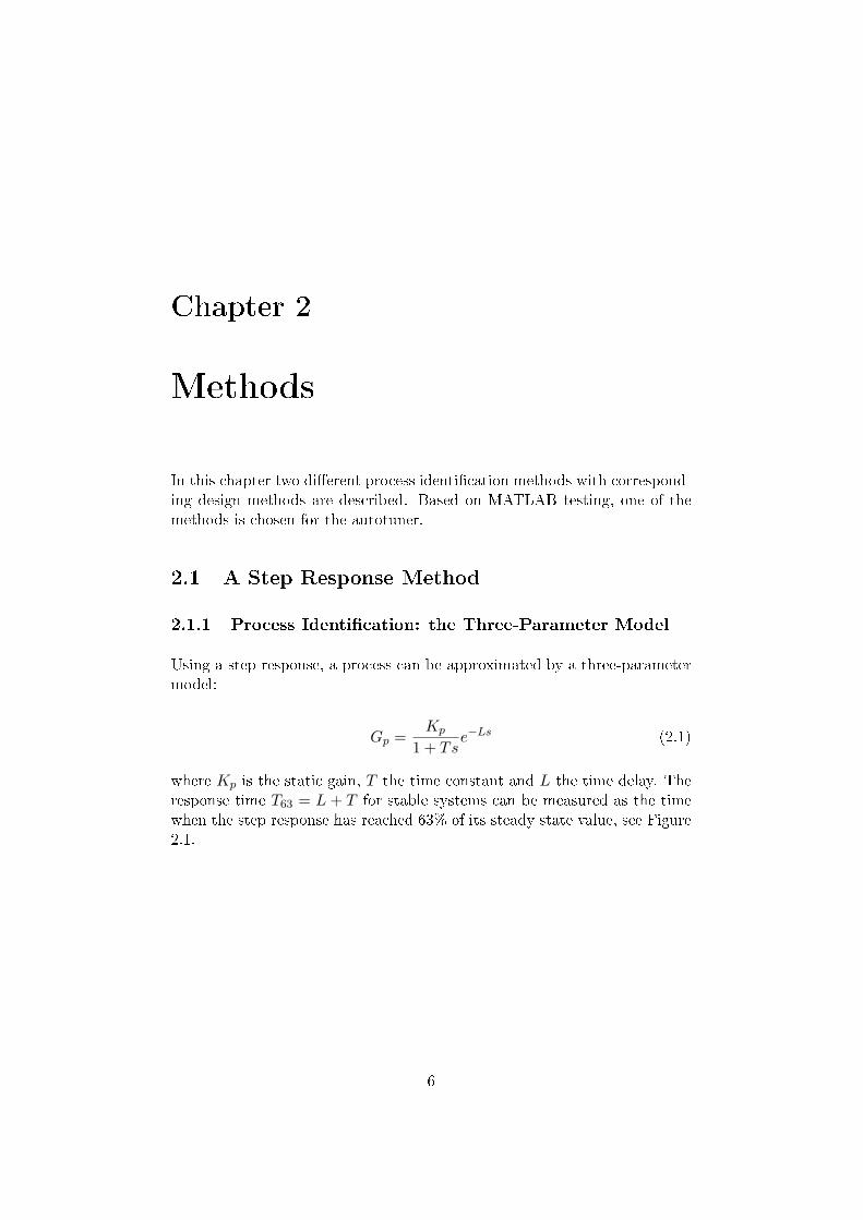
Using a step response, a process can be approximated by a three-parametermodel:

Gp =Kp

1 + Tse−Ls (2.1)

where Kp is the static gain, T the time constant and L the time delay. Theresponse time T63 = L + T for stable systems can be measured as the timewhen the step response has reached 63% of its steady state value, see Figure2.1.

6

CHAPTER 2. METHODS 7

Figure 2.1: The response time T63 = T + L.

There are several di�erent ways to determine Kp, T and L; three of themare described below.

Estimating the delay

One way is to estimate the delay L by measuring when the measurementsignal is starting to increase. From the response time T63 and the estimateddelay L, the time constant T can be calculated as T = T63 − L. The staticgain Kp is calculated as:

Kp =yfinal − ybegin

ufinal − ubegin(2.2)

where u is the control signal and y is the measurement signal

Ziegler-Nichols step response method

Another method is the Ziegler-Nichols step response method where the delayL can be estimated by using the maximum slope tangent of the step response.Using this tangent it is possible to �nd two points, one on the horizontalaxis and one on the vertical axis. The delay is the time from the start of thestep to the point where the tangent is crossing the horizontal axis. A newparameter, a, is introduced as the di�erence between the initial value andthe tangent crossing the vertical axis. From these two parameters togetherwith the static gain the relationship

a =KpL

T(2.3)


can be used to �nd T . Kp is calculated as in Equation 2.2.

Method of Moments

A third way to determine Kp , T and L is the Method of Moments describedin [2]. The area A0 is the integrated distance between the stationary endlevel of y and the measurement signal y in an open loop step. The areaA0/k, also called Tar, can be used as a good estimate of T63 for the three-parameter model, see article [3]. The area A1 beneath the step response isalso integrated. The areas are shown in Figure 2.2.

Figure 2.2: A step response in open loop with the areas used in Method of Mo-

ments.

The area A1 is used to calculate the time constant:

T =eA1

hKp(2.4)

and the area A0 is used to calculate the delay:

L = Tar − T =A0

hKp− eA1

hKp(2.5)

h is the step amplitude of the control signal and Kp is the static gain fromEquation 2.2.

The approximated processes yielded by these three di�erent methods weresimulated in MATLAB and were compared with the original process. Theconclusion was that the Method of Moments gives the best approximation.


2.1.2 Design Method

When the parameters Kp, T and L are known a design method can be chosento transform them into PI-parameters or PID-parameters. One such methodis the well-known Ziegler-Nichols' set of tuning rules. A modern method isthe AMIGO tuning rules proposed in [3]. It uses the following equations:

K =1

Kp(0.2 + 0.45T/L)

Ti =0.4L + 0.8T

L + 0.1TL (2.6)

Td =0.5LT

0.3L + T

Instead of only using two parameters, a and L like the Ziegler-Nichols tuningrules, the AMIGO tuning rules are based on three parameters, Kp, T andL. The AMIGO method has been developed with a robustness constraintand it uses a dependency on the normalized dead time τ = L/(L+T ) unlikethe Ziegler-Nichols tuning rules. The AMIGO method suits a large variationof processes and seems to be more universal than the Ziegler-Nichols tuningrules.

The AMIGO design method recommends a setpoint weighting which dependson τ , this is not used since the setpoint weighting is not changeable in thePIDP-block. The PIDP-block has its own setpoint weighting de�nition: b =0 for PI and PID-control and b = 1 for P and PD-control.

2.1.3 The Method of Moments in Practice

A variation of the Method of Moments described in [2], which is furtherdeveloped in [4] is used.

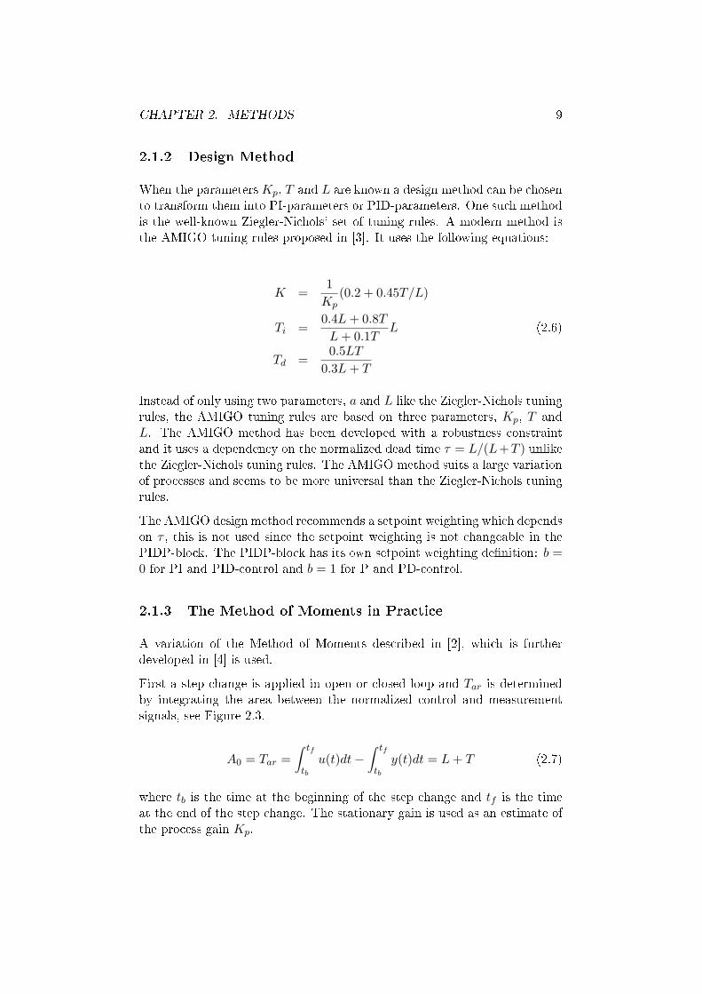
First a step change is applied in open or closed loop and Tar is determinedby integrating the area between the normalized control and measurementsignals, see Figure 2.3.

A0 = Tar =∫ tf

tb

u(t)dt−∫ tf

tb

y(t)dt = L + T (2.7)

where tb is the time at the beginning of the step change and tf is the timeat the end of the step change. The stationary gain is used as an estimate ofthe process gain Kp.


Figure 2.3: A step response in closed loop with the normalized control and mea-

surement signal.

A second step change in opposite direction is then applied in open loop andthe area A1 of the step response is calculated during the time Tar. The timeconstant T is then calculated as in Equation 2.4 and the delay L is equal toTar − T .

The Method of Moments can be executed in both open loop and closed loop.A closed loop is known to take care of process disturbances but requiressome safe default values for the PID-parameters of the controller. Whenusing closed loop, one must be aware that a high gain can cause instabilityproblems when the process has long delays. With an open loop, it is di�cultto be sure that the step amplitude is appropriate. An unknown high gaincan lead to unforeseen consequences in the process output.

This area-method is easy to automate since calculation of the areas throughintegration can be done online. It is also robust to high-frequency distur-bances since erroneous measurements during the integration process shouldcancel each other out due to the low pass nature of integration.

A lot of tests have been performed on di�erent types of processes. Themajor test objective was to see if the new controller parameters improvedthe performance of the control loop. The range of tested processes includes�rst-order and higher-order processes as well as processes with small andlarge time constants and delays.

The tests were performed in SIMULINK. The Method of Moments was au-tomated using an S-function. The AMIGO design method mentioned abovein Equation 2.6 was used with the approximated parameters Kp, T and L. Astep response of each process controlled with safe default PI-parameters anda step response of the same process controlled with the new PID-parameterswere compared. The new controller parameters give a fast step responsewith an acceptably small overshoot.


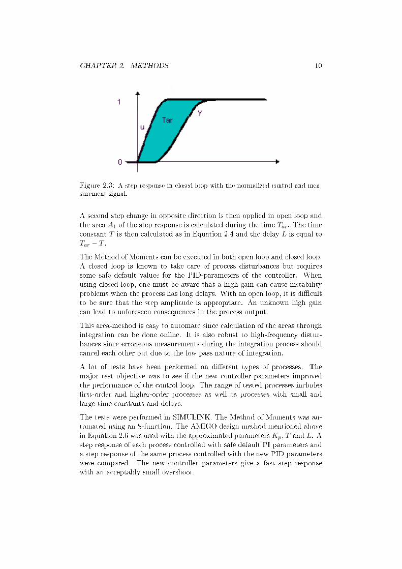
2.2 The Relay Feedback Method

Figure 2.4: Relay feedback loop.

2.2.1 Process Identi�cation

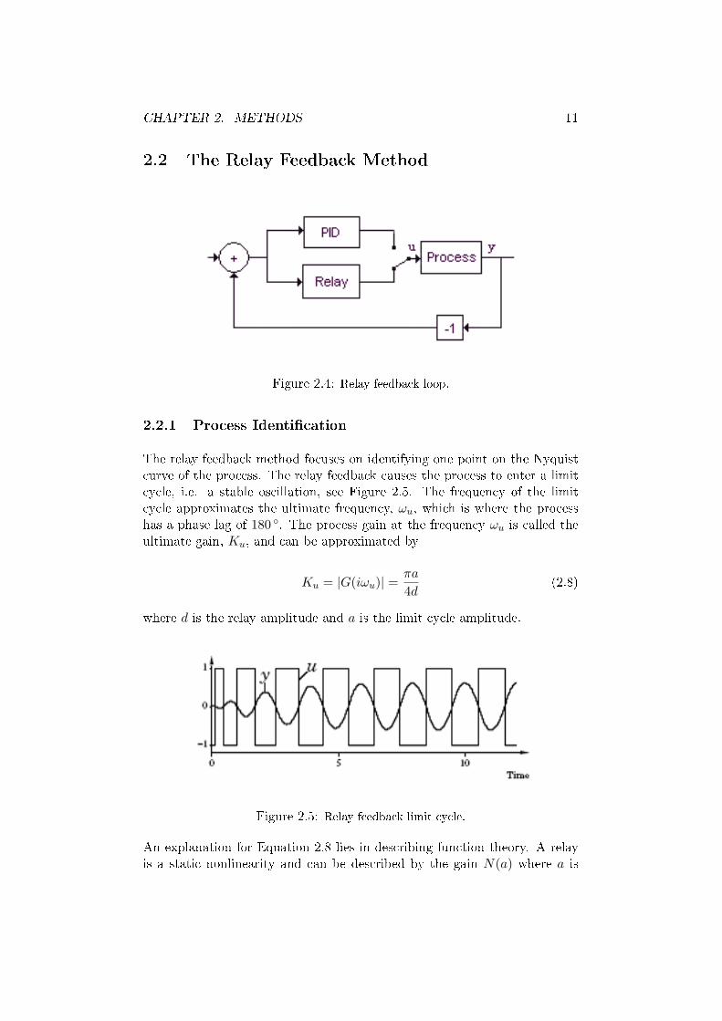
The relay feedback method focuses on identifying one point on the Nyquistcurve of the process. The relay feedback causes the process to enter a limitcycle, i.e. a stable oscillation, see Figure 2.5. The frequency of the limitcycle approximates the ultimate frequency, ωu, which is where the processhas a phase lag of 180 ◦. The process gain at the frequency ωu is called theultimate gain, Ku, and can be approximated by

Ku = |G(iωu)| = πa

4d(2.8)

where d is the relay amplitude and a is the limit cycle amplitude.

Figure 2.5: Relay feedback limit cycle.

An explanation for Equation 2.8 lies in describing function theory. A relayis a static nonlinearity and can be described by the gain N(a) where a is


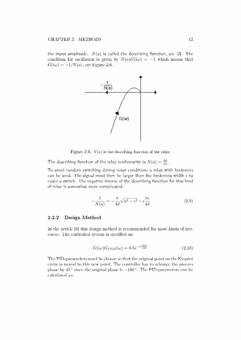
the input amplitude. N(a) is called the describing function, see [2]. Thecondition for oscillation is given by N(a)G(iω) = −1 which means thatG(iω) = −1/N(a), see Figure 2.6.

Figure 2.6: N(a) is the describing function of the relay.

The describing function of the relay nonlinearity is N(a) = 4dπa .

To avoid random switching during noisy conditions a relay with hysteresiscan be used. The signal must then be larger than the hysteresis width ε tocause a switch. The negative inverse of the describing function for this kindof relay is somewhat more complicated:

− 1N(a)

= − π

4d

√a2 − ε2 − i

πε

4d(2.9)

2.2.2 Design Method

In the article [6] this design method is recommended for most kinds of pro-cesses. The controlled system is speci�ed as:

G(iω)GPID(iω) = 0.5e−i 135π180 (2.10)

The PID-parameters must be chosen so that the original point on the Nyquistcurve is moved to this new point. The controller has to advance the processphase by 45 ◦ since the original phase is −180 ◦. The PID-parameters can becalculated as:


K =0.5 cos 45 ◦

Ku

Td =tan 45 ◦ +

√4α + tan2 45 ◦

2ωu(2.11)

Ti = αTd

where α = 6.25 according to [6].

2.2.3 The Relay Feedback Method in Practice

The relay method as described above is easy to automate. The output fromthe process is measured and when a stable limit cycle is detected its periodtime and amplitude are measured and averaged over several cycles. Theperiod time gives the ultimate frequency ωu and the amplitude a is used tocalculate Ku as in Equation 2.8.

The method has been tested on a range of processes similar to the onestested in part 2.1.3. The design method described in Equation 2.11 was used.Tests have been performed using SIMULINK and the process identi�cationand design are both implemented in an S-function. A step response of eachprocess controlled with safe default PI-parameters and a step response ofthe same process controlled with the new PID-parameters were compared.The immediate conclusion is that the design method does not give very goodresults for most of the tested processes. For processes including a substantialdelay the control is very slow and ine�cient and processes with large timeconstants receive a very large K.

The process delay could be approximated during the experiment and anappropriate design method chosen according to the result. In article [6] aPI-design is recommended for processes with delays.

2.3 Discussion

The step response method, represented by the Method of Moments, and therelay feedback method are both easy to automate. Positive aspects of theMethod of Moments are that it is robust against high frequency disturbancesand safe if the �rst step change is made in a closed loop. If the �rst stepchange is made in open loop it means taking a risk with the system. Therelay feedback method is executed in a closed loop and is also safe for thesystem.


The decision of which method to choose is based on the test results with thenew PID-parameters. The parameters generated with Method of Momentsgive fast step responses with a small overshoot. The parameters generatedwith the relay feedback method do not give so good step responses. Depend-ing on the process characteristics the step responses are either very slow orhave large overshoots. To get better results, a step change could be addedto the relay feedback method to �nd the static gain of the unknown process.Then the PID-design could be based on three parameters instead of onlytwo, Ku and ωu. The process delay L could also be approximated. Basedon L a decision could be made in the design phase on whether to use PID orPI-control. Since the Method of Moments together with the AMIGO designalready gives good results this will be the method used in the autotuner.

Chapter 3

Implementation

3.1 IEC 61131 and PLC programming in CoDeSys

The autotuner is implemented in the IEC 61131 standard. IEC 61131 hasbeen developed for PLC application programming in the automation indus-try. It contains several languages as follows:

• Instruction List (IL)

• Structured Text (ST)

• Sequential Function Charts (SFC)

• Function Block Diagram (FBD)

• Ladder Diagram (LD)

The �rst two languages, IL and ST, are text based. IL is an assembly-likelanguage while ST resembles Pascal. The other languages are graphical lan-guages, which means that applications are described using di�erent blocksconnected to each other. An IEC 61131 application can be created usingany combination of these languages. The concept of hierarchy is well devel-oped which means that an application can be highly structured. Blocks cancontain applications written in any of the languages mentioned above.

The most specialised language in IEC 61131 is SFC, which is used to describesequential behaviour. This is very useful for control applications since theyare often time- and/or event-driven. A SFC application is built using stepsand transitions. The steps represent the states in the control �ow. Thetransitions are conditions that allow state change. A transition can onlyoccur if the step immediately before the transition is active. Concurrent aswell as alternative sequences of steps are allowed.

15

CHAPTER 3. IMPLEMENTATION 16

The IEC 61131 programming tool used for implementation of the autotuneris called CoDeSys, Controller Development System, by Smart Software So-lutions.

3.2 Overview of the Implementation

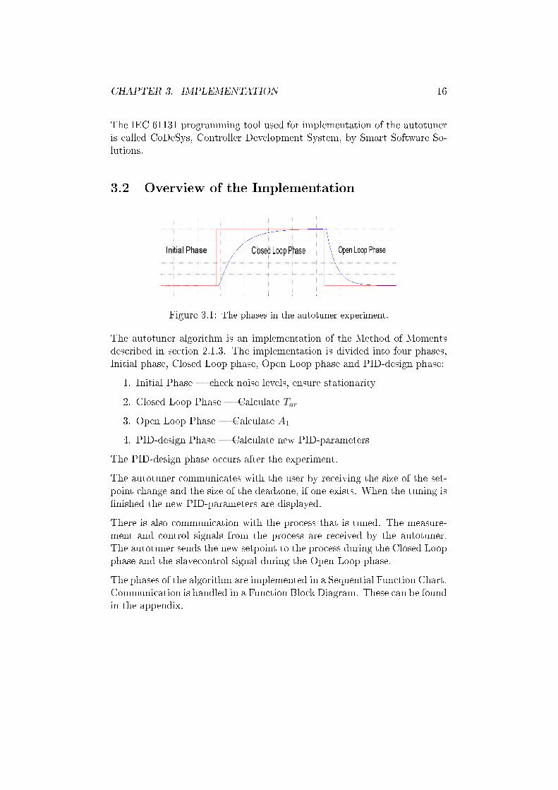
Figure 3.1: The phases in the autotuner experiment.

The autotuner algorithm is an implementation of the Method of Momentsdescribed in section 2.1.3. The implementation is divided into four phases,Initial phase, Closed Loop phase, Open Loop phase and PID-design phase:

1. Initial Phase � check noise levels, ensure stationarity

2. Closed Loop Phase � Calculate Tar

3. Open Loop Phase � Calculate A1

4. PID-design Phase � Calculate new PID-parameters

The PID-design phase occurs after the experiment.

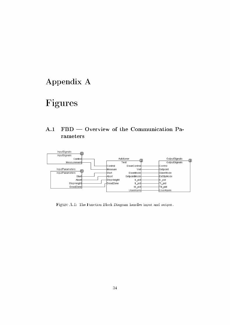
The autotuner communicates with the user by receiving the size of the set-point change and the size of the deadzone, if one exists. When the tuning is�nished the new PID-parameters are displayed.

There is also communication with the process that is tuned. The measure-ment and control signals from the process are received by the autotuner.The autotuner sends the new setpoint to the process during the Closed Loopphase and the slavecontrol signal during the Open Loop phase.

The phases of the algorithm are implemented in a Sequential Function Chart.Communication is handled in a Function Block Diagram. These can be foundin the appendix.


3.3 Detailed Implementation

3.3.1 Initial Phase

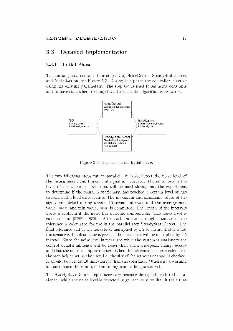
The Initial phase contains four steps, Go, NoiseDetect, SteadyStateDetectand Initialization, see Figure 3.2. During this phase the controller is activeusing the existing parameters. The step Go is used to set some constantsand to have somewhere to jump back to when the algorithm is restarted.

Figure 3.2: The steps in the Initial phase.

The two following steps run in parallel. In NoiseDetect the noise level ofthe measurement and the control signal is measured. The noise level is thebasis of the tolerance level that will be used throughout the experimentto determine if the signal is stationary, has reached a certain level or hasexperienced a load disturbance. The maximum and minimum values of thesignal are picked during several 15-second intervals and the average maxvalue, max, and min value, mın, is computed. The length of the intervalsposes a problem if the noise has periodic components. The noise level iscalculated as |max − mın|. After each interval a rough estimate of thetolerance is calculated for use in the parallel step SteadyStateDetect. The�nal tolerance will be the noise level multiplied by 1.2 to ensure that it is nottoo sensitive. If a dead zone is present the noise level will be multiplied by 1.5instead. Since the noise level is measured while the system is stationary thecontrol signal's in�uence will be lesser than when a setpoint change occursand thus the noise will appear lesser. When the tolerance has been calculatedthe step height set by the user, i.e. the size of the setpoint change, is checked.It should be at least 10 times larger than the tolerance. Otherwise a warningis issued since the results of the tuning cannot be guaranteed.

The SteadyStateDetect step is necessary because the signal needs to be sta-tionary while the noise level is detected to get accurate results. It tests that


the measurement signal is stationary for 60 seconds by checking if it stays atthe same level, which means that it does not change more than the tolerancelevel allows. 60 seconds is an arbitrarily chosen time period which seems towork. It means that the NoiseDetect step has four intervals to compute thenoise level average from. The measurement signal is averaged online and thelatest sample is compared with the average. If the di�erence is larger thanthe tolerance level for more than two samples in a row both the NoiseDe-tect and SteadyStateDetect steps are restarted. Allowing divergence for twosamples takes care of sporadic outliers so that unnecessary restarts will notoccur too often.

The last step in the Initial phase is called Initialization. Its main purpose isto determine good values for the initial levels of the control and measurementsignals. The initial levels will be used later in the experiment. The sametest as in SteadyStateDetect is performed to see if the signals are station-ary, and the tolerance now has the value determined in NoiseDetect. Whenstationarity has lasted for half the time compared to SteadyStateDetect, i.e.30 seconds, the averages of the control and measurement signals are deemedto be stable enough. If stationarity is interrupted, the procedure will berepeated including the two previous steps.

3.3.2 Closed Loop Phase

Figure 3.3: The initial and end levels for the control and measurement signals.

A step change is made with the controller active using existing parameters.The dead zone parameter, described in section 1.1, will contribute to a sta-


tionary level that di�ers slightly from the setpoint. The stationary leveldepends on the controller PI-parameters, slow parameters get a lower leveland fast parameters get a higher level than the setpoint. For reaching thesetpoint with slow PI-parameters the dead zone is added to the step sizewhen computing the setpoint.

The step direction is set by the user in the beginning of the experiment withthe step size. A negative step size gives a closed step in downward directionand a positive step size gives a closed step in upward direction.

The areas of the measurement and control signals are computed as Riemann-sums, using the sample time.

The delay is measured as the time until the signal passes 1% of the stepchange and is later used in the PID-design phase.

T63, the time it takes to reach 63% of the step change, is measured and twicethis time gives a time-limit for how long the system should remain stationaryafter reaching its new level. This time-limit should not be too short sinceslow step responses risk being interrupted too early, before the level is reallyreached. The time-limit should not be too long either, considering that thedisturbance probability will increase. When a dead zone exists the param-eter T63 is badly approximated, but still gives a long enough time-limit forreaching stationarity. When the measurement signal reaches T63 a booleanvariable is set true and when 1/4 of the time-limit has passed the algorithmallows two samples in sequence to be out of range for the tolerance level.These samples are excluded when computing the average for the end level ofthe step response.

When the condition for stationarity fails the algorithm will check for load dis-turbances, see section 3.3.5. If a load disturbance has occurred the algorithmwill be terminated. The algorithm will also be terminated if the worst-casetime for the step change has passed. A normal Closed Loop phase is esti-mated to take less than 2 · T63 + time-limit seconds, the worst-case time forthe closed loop is set to twice the normal phase time. To check the controlsignal the only thing that is known in this phase is the initial level. If thecontrol signal has opposite direction to the step change and has passed itsinitial level the algorithm will terminate.

Finally, when the stationarity condition is ful�lled, Tar is computed by takingthe di�erence of the normalized signal areas. Tar is used in the next phase asthe expected response time for an open loop step change, which correspondsto T63 for the closed loop step change. Checks to see that the control signaldoes not saturate are also performed. The level of the actual step change iscompared with the one set by the user in the beginning of the experimentand checked against the noise amplitude.


3.3.3 Open Loop Phase

The controller is deactivated and the algorithm sets the control signal to itsinitial level. This will result in an open loop step in the opposite directionto the closed loop step.

The area of the measurement signal is computed until the response time isreached, see Figure 3.6. The total area of the signal is also computed, andwill be compared with Tar from the previous phase.

The delay in this phase is estimated as the time until the measurement signalchanges direction from the stationary level. This delay will later be comparedwith the approximated delay in the PID-design phase.

A new time-limit for the measurement signal being stationary when theinitial level has been reached is calculated as twice the response time. Anaverage of the measurement signal is computed when the signal is stationary,in the same way as in the other phases. This average will be compared to theinitial level computed in the Initial phase, and will be used as an accuracyparameter for the experiment in the PID-design phase.

If the stationary condition depending on the tolerance level fails, the algo-rithm will check if a load disturbance has occurred, see section 3.3.5.

3.3.4 PID-design Phase

The approximations of Kp, T and L are calculated using the areas computedin the Closed Loop and Open Loop phases. Using the approximations thenew PID-parameters are calculated by using the AMIGO tuning rules de-scribed in the Equation 2.6. Then the credibility of the parameters is judged.For now the only check performed is that they should be non-negative.

3.3.5 Disturbance Detection

Initial Phase

A load disturbance in the Initial phase makes the measurement signal loosecontact with the setpoint during the time it takes for the control signal tocompensate for the error. When the measurement signal is stabilized thecontrol signal gets a new initial level to keep the measurement signal at thesetpoint. If the control signal does not saturate the experiment will go onwithout in�uencing the result.

A pulse disturbance will make the measurement signal loose its setpoint fora while and then the signals will return to their initial levels.


When a load or pulse disturbance occurs in the Initial phase, no speci�c dis-turbance detection algorithm is used. Instead the steady state detection isrestarted and a limitation of the remaining experiment time is used to avoidin�nite loop.

Closed Loop Phase

Disturbances in this phase will destroy the integration of the signal areas.The di�erence between the normalized signal areas, Tar, is later used in theOpen Loop phase as an estimate for the response time. The approximation ofthe three-parameter model, described in Equation 2.1, depends on a correctlyestimated response time for computing the area A1 in the Open Loop phase.

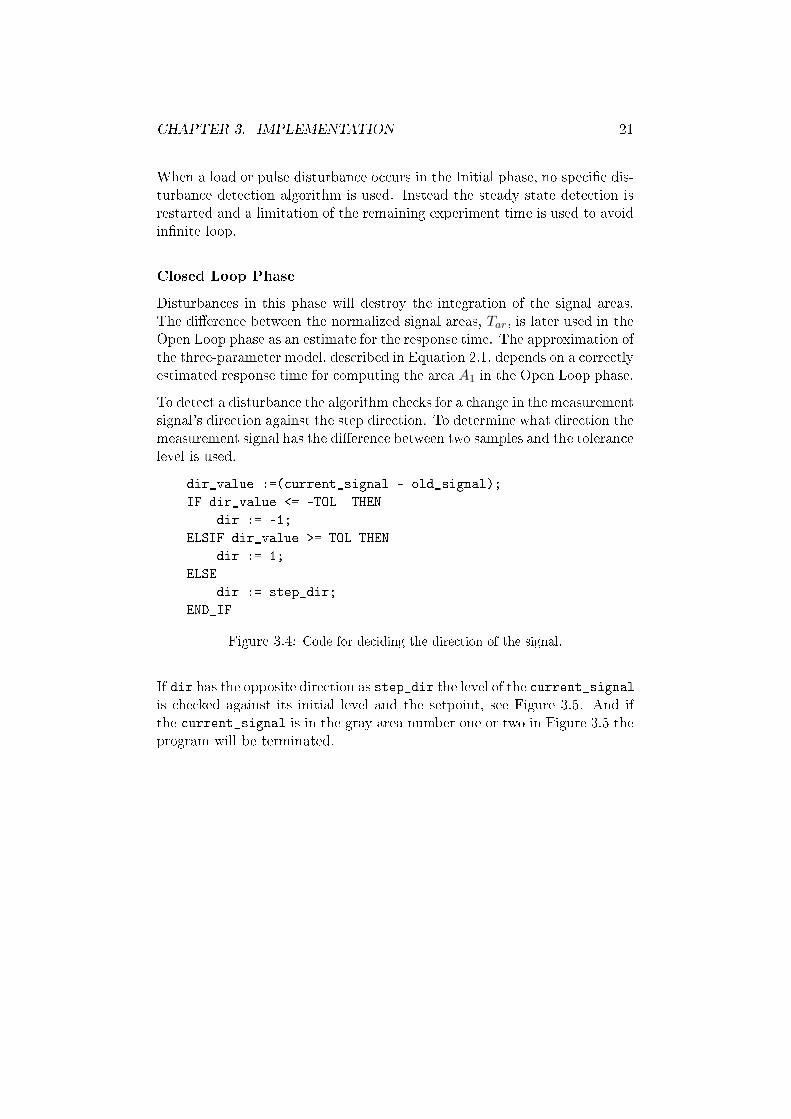
To detect a disturbance the algorithm checks for a change in the measurementsignal's direction against the step direction. To determine what direction themeasurement signal has the di�erence between two samples and the tolerancelevel is used.

dir_value :=(current_signal - old_signal);

IF dir_value <= -TOL THEN

dir := -1;

ELSIF dir_value >= TOL THEN

dir := 1;

ELSE

dir := step_dir;

END_IF

Figure 3.4: Code for deciding the direction of the signal.

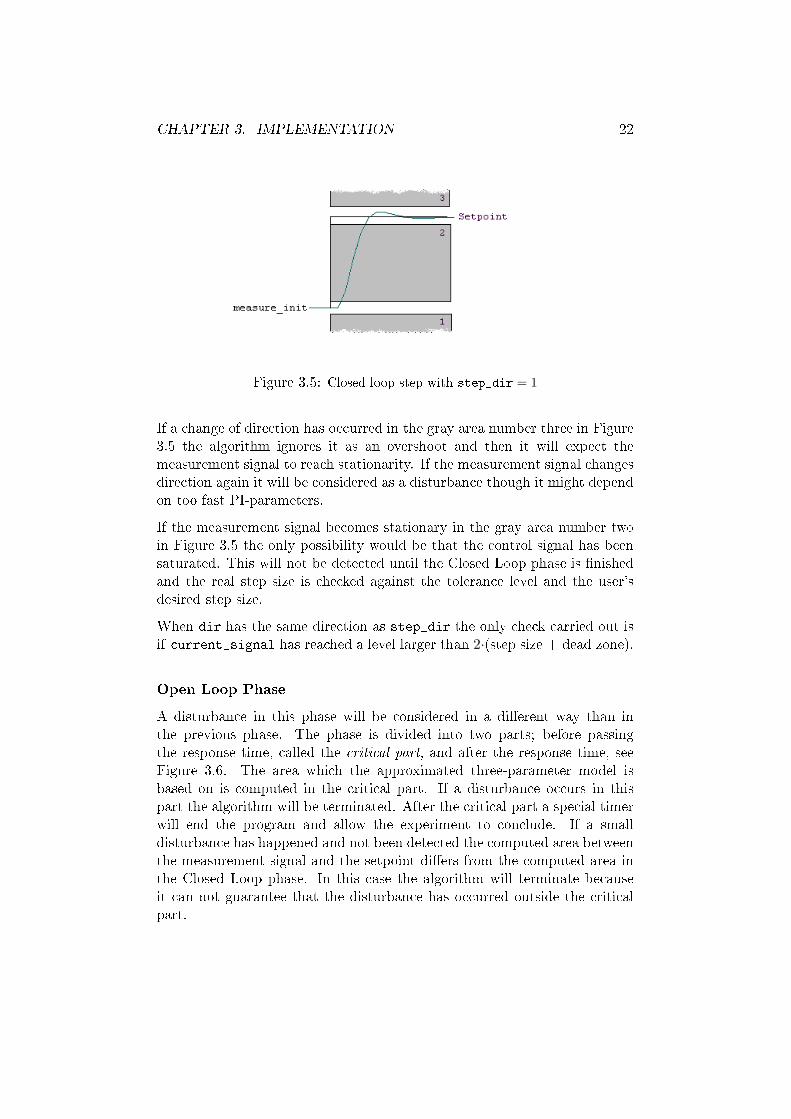
If dir has the opposite direction as step_dir the level of the current_signalis checked against its initial level and the setpoint, see Figure 3.5. And ifthe current_signal is in the gray area number one or two in Figure 3.5 theprogram will be terminated.


Figure 3.5: Closed loop step with step_dir = 1

If a change of direction has occurred in the gray area number three in Figure3.5 the algorithm ignores it as an overshoot and then it will expect themeasurement signal to reach stationarity. If the measurement signal changesdirection again it will be considered as a disturbance though it might dependon too fast PI-parameters.

If the measurement signal becomes stationary in the gray area number twoin Figure 3.5 the only possibility would be that the control signal has beensaturated. This will not be detected until the Closed Loop phase is �nishedand the real step size is checked against the tolerance level and the user'sdesired step size.

When dir has the same direction as step_dir the only check carried out isif current_signal has reached a level larger than 2·(step size + dead zone).

Open Loop Phase

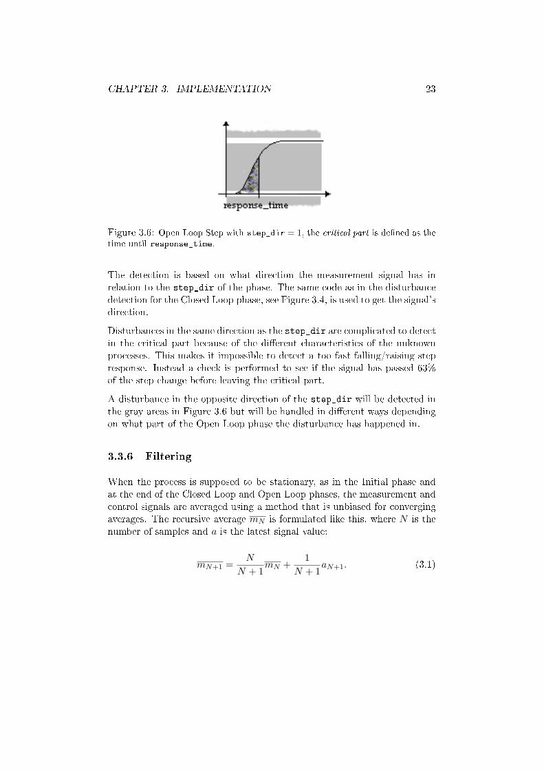
A disturbance in this phase will be considered in a di�erent way than inthe previous phase. The phase is divided into two parts; before passingthe response time, called the critical part, and after the response time, seeFigure 3.6. The area which the approximated three-parameter model isbased on is computed in the critical part. If a disturbance occurs in thispart the algorithm will be terminated. After the critical part a special timerwill end the program and allow the experiment to conclude. If a smalldisturbance has happened and not been detected the computed area betweenthe measurement signal and the setpoint di�ers from the computed area inthe Closed Loop phase. In this case the algorithm will terminate becauseit can not guarantee that the disturbance has occurred outside the criticalpart.


Figure 3.6: Open Loop Step with step_dir = 1, the critical part is de�ned as the

time until response_time.

The detection is based on what direction the measurement signal has inrelation to the step_dir of the phase. The same code as in the disturbancedetection for the Closed Loop phase, see Figure 3.4, is used to get the signal'sdirection.

Disturbances in the same direction as the step_dir are complicated to detectin the critical part because of the di�erent characteristics of the unknownprocesses. This makes it impossible to detect a too fast falling/raising stepresponse. Instead a check is performed to see if the signal has passed 63%of the step change before leaving the critical part.

A disturbance in the opposite direction of the step_dir will be detected inthe gray areas in Figure 3.6 but will be handled in di�erent ways dependingon what part of the Open Loop phase the disturbance has happened in.

3.3.6 Filtering

When the process is supposed to be stationary, as in the Initial phase andat the end of the Closed Loop and Open Loop phases, the measurement andcontrol signals are averaged using a method that is unbiased for convergingaverages. The recursive average mN is formulated like this, where N is thenumber of samples and a is the latest signal value:

mN+1 =N

N + 1mN +

1N + 1

aN+1. (3.1)

Chapter 4

Test Results

The autotuner has been tested on three �rst-order processes with di�erentcharacteristics, one lag dominated, one delay dominated and one balancedprocess. Lag dominated means that the process time constant T is muchlarger than the process delay L and τ is small. Delay dominated means thatL > T and τ is large. τ is calculated as L

L+T and used as a basis for theAMIGO tuning rules, see section 2.1.2.

To show the further capabilities of the autotuner, it has also been tested ona �rst-order balanced process with measure noise and dead zone.

The tests have been performed using processes simulated with TAC Menta,a FBD programming tool used by TAC to implement control applications.

"Original" PI-parameters that give a slow step response without overshootsare chosen for each process. New PID-parameters are generated with theautotuner and tested with a step response. Then T63, the time it takes toreach 63% of the step height, for the new parameters is compared with T63

for the "original" parameters.

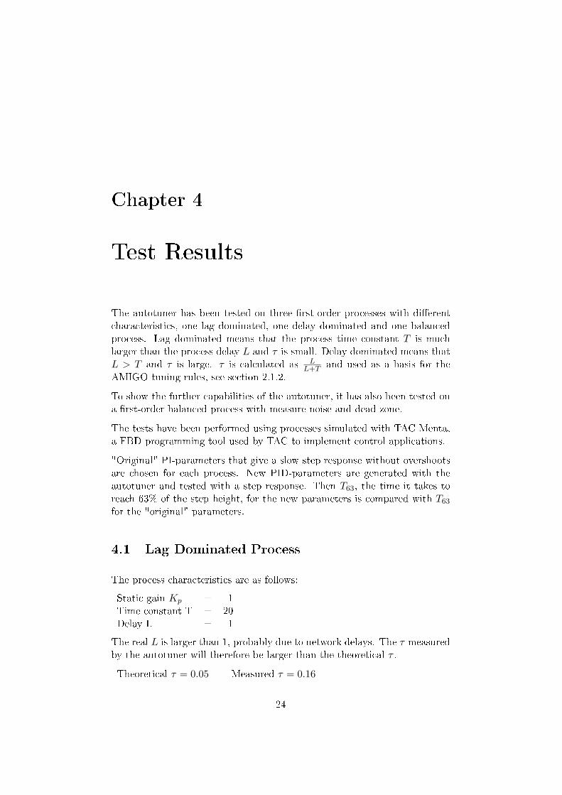
4.1 Lag Dominated Process

The process characteristics are as follows:

Static gain Kp = 1Time constant T = 20Delay L = 1

The real L is larger than 1, probably due to network delays. The τ measuredby the autotuner will therefore be larger than the theoretical τ .

Theoretical τ = 0.05 Measured τ = 0.16

24

CHAPTER 4. TEST RESULTS 25

The original and new PID-parameters are compared as well as T63.

Original PI-parameters: New PID-parameters:K = 0.5Ti = 15.0Td = 0

T63 = 49s

K = 2.58Ti = 10.40Td = 1.63

T63 = 18s

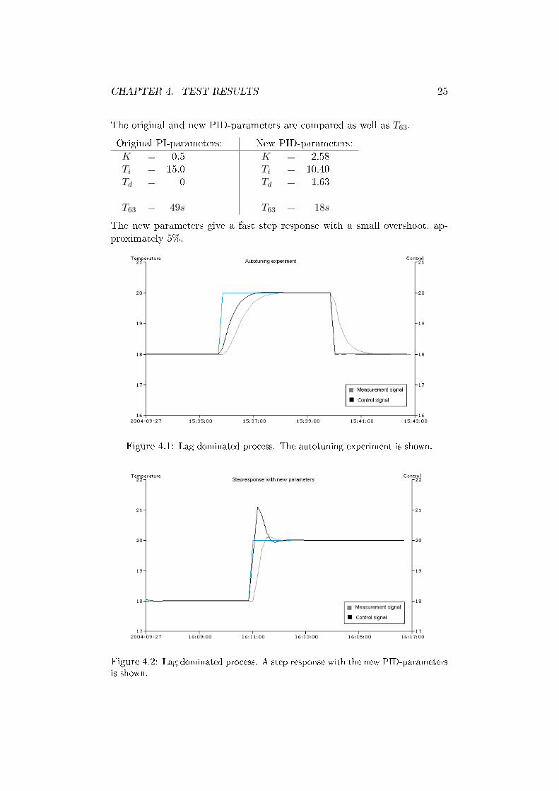
The new parameters give a fast step response with a small overshoot, ap-proximately 5%.

Figure 4.1: Lag dominated process. The autotuning experiment is shown.

Figure 4.2: Lag dominated process. A step response with the new PID-parameters

is shown.


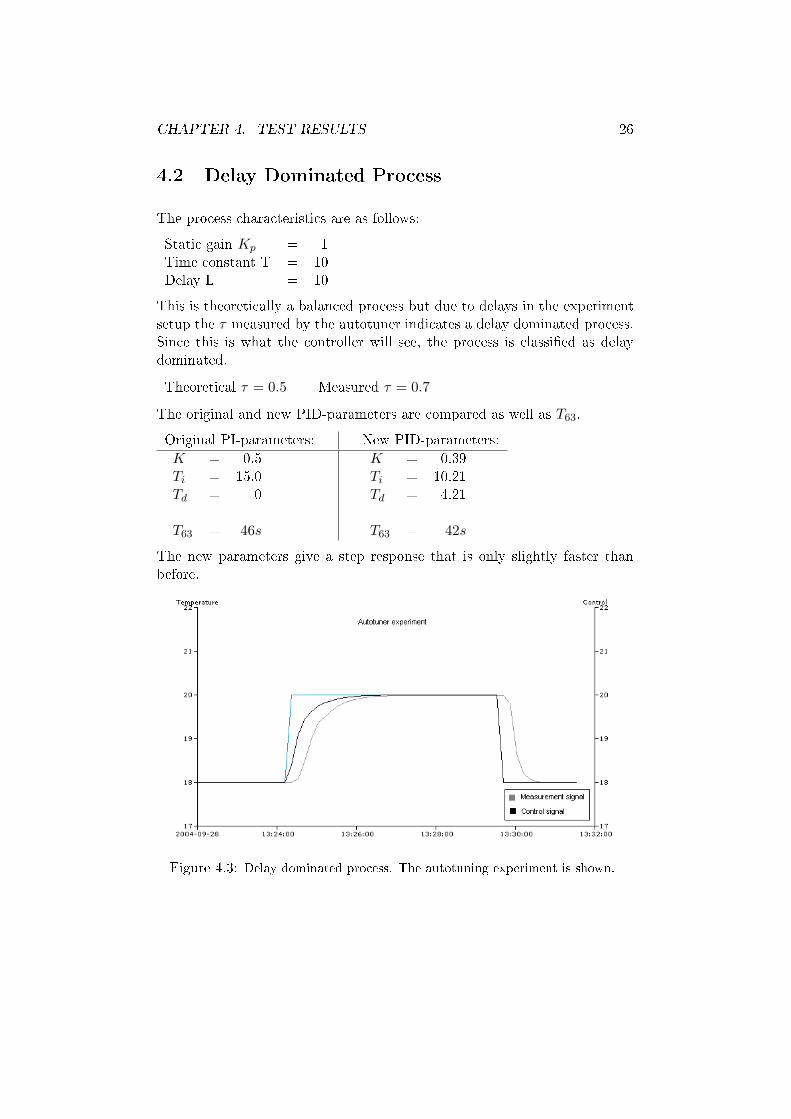
4.2 Delay Dominated Process



This is theoretically a balanced process but due to delays in the experimentsetup the τ measured by the autotuner indicates a delay dominated process.Since this is what the controller will see, the process is classi�ed as delaydominated.




T63 = 46s

K = 0.39Ti = 10.21Td = 4.21

T63 = 42s

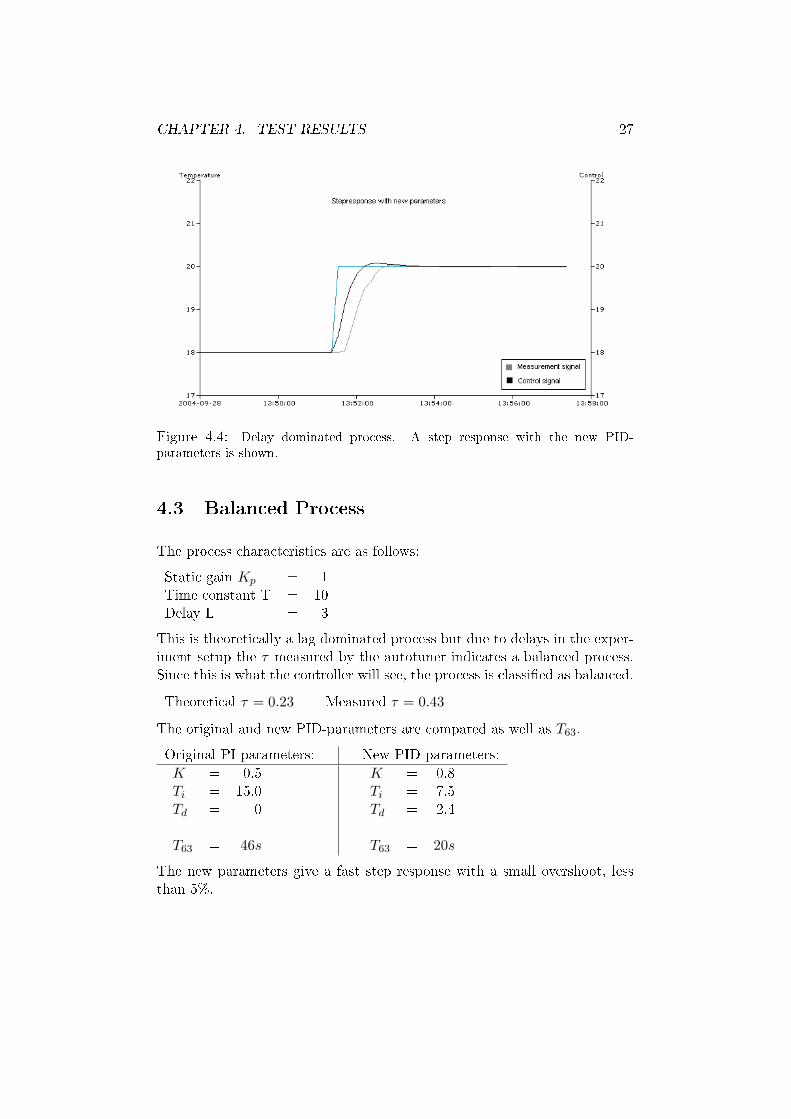
The new parameters give a step response that is only slightly faster thanbefore.

Figure 4.3: Delay dominated process. The autotuning experiment is shown.


Figure 4.4: Delay dominated process. A step response with the new PID-

parameters is shown.

4.3 Balanced Process



This is theoretically a lag dominated process but due to delays in the exper-iment setup the τ measured by the autotuner indicates a balanced process.Since this is what the controller will see, the process is classi�ed as balanced.




T63 = 46s

K = 0.8Ti = 7.5Td = 2.4

T63 = 20s

The new parameters give a fast step response with a small overshoot, lessthan 5%.


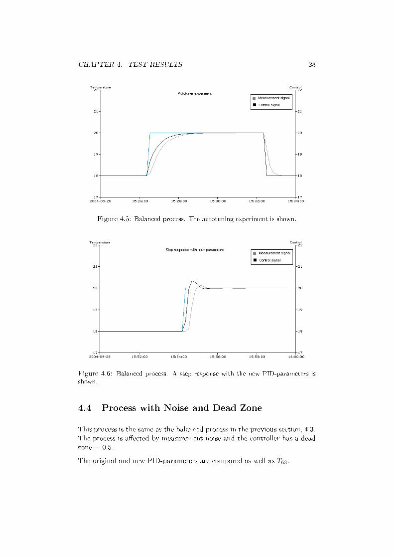
Figure 4.5: Balanced process. The autotuning experiment is shown.

Figure 4.6: Balanced process. A step response with the new PID-parameters is

shown.

4.4 Process with Noise and Dead Zone

This process is the same as the balanced process in the previous section, 4.3.The process is a�ected by measurement noise and the controller has a deadzone = 0.5.




T63 = 45s

K = 0.51Ti = 6.41Td = 2.51

T63 = 23s

The new parameters give a fast step response with an overshoot, approxi-mately 5%. The signal levels di�er from the setpoint because of the deadzone.

Figure 4.7: Balanced process with noise and dead zone. The autotuning experi-

ment is shown.

Figure 4.8: Balanced process with noise and dead zone. A step response with the

new PID-parameters is shown.


4.5 Testing on an Air Handling Unit

The autotuner has also been tried with the heating process of an air han-dling unit. It was found that it is hard to bring the process to stationarity,which is a prerequisite for the tuning experiment. Another problem is thatthe outdoor temperature can change during the experiment and disturb theresults.

The autotuner makes one upwards and one downwards step change. It ispossible that the process has di�erent dynamics going up or down. Thisproblem could be avoided by making both step changes in the same direction.

Real processes are not linear and time invariant as the simulated processesare. This leads to a lot of interesting problems when trying to apply theautotuner. These problems will have to be taken care of in future versions.

Chapter 5

Conclusions

5.1 Summary

An autotuner based on the Method of Moments combined with the AMIGOtuning rules has been built. It has been tested on various processes andthe generated PID-parameters give fast step responses with acceptable over-shoots. It is hard to tell if the parameters are optimal but at least they givegood results.

During testing we have noticed that the approximations of the process pa-rameters T and L are often far from the original parameters. However, T +Lis close to the mark. Even though the approximations are bad, the resultingPID-parameters give good step responses.

The total time of an experiment depends on the controller parameters usedand the nature of the process that is tuned. The autotuner uses two stepscompared to manual tuning which might need several steps to achieve goodcontroller parameters. This makes the autotuner time-economical when newparameters are needed.

In some experiments the controller parameters given by the autotuner resultin an oscillating step response. This could be because some undetecteddisturbance has occured or it could depend on communication problems.The user should therefore assess the parameters before deploying them.

5.2 User Notes

Some basic knowledge about the process that will be tuned and a bit ofcontrol theory will still be needed for the user of the autotuner.

31

CHAPTER 5. CONCLUSIONS 32

The autotuner should be connected to one PID-controller at the time, notto entire cascaded control loops.

Before running the autotuner the user should make sure that the system iscontrolled with slow and safe PID-parameters, giving a step response withoutovershoot. The system should also be in steady state.

The step size of the experiment should be su�ciently large, at least 20 timesthe approximated noise amplitude. If a dead zone is present in the process,the user must state its size.

The experiment will take at least as much time as two setpoint changes.If the experiment is interrupted an error message will be displayed withinformation about the possible cause. Load disturbances that occur duringthe experiment will invalidate the results and the autotuner therefore triesto detect them and interrupt the experiment.

When the experiment concludes, the new PID-parameters are displayed.They can then be manually transferred to the PID-controller.

Most of TACs control systems use only the proportional and integral partsof the PID-controllers. The autotuner will in most cases propose that thecontroller uses the derivative part as well. When the derivative part is usedthe system will become more sensitive to high frequency disturbances andtherefore a lowpass �lter should be used.

The autotuner will give optimal parameters, but the parameters will onlyremain optimal as long as system conditions remain unchanged. A tuning ofa temperature control system that takes place during winter will probablynot give parameters suitable for summer control.

5.3 Future Work

• Better identi�cation and �ltering of the measurement noise.

• Check the generated PID-parameters to see if they seem probable.Checks can be added, such as comparing the di�erent Tar:s calculatedin the Closed Loop and Open Loop phases, comparing the measured Lwith the calculated L and checking what non-fatal errors have occurred.

• Use τ to make further adjustments to the PID-parameters as describedin article [3].

• Use τ to adjust the setpoint weighting of the controller, according to[3].

CHAPTER 5. CONCLUSIONS 33

• Save the information from previous tuning experiments and use it toget better process identi�cation.

• Use the autotuner to generate several parameter sets for use in gainscheduling.

• Further development and testing to make the autotuner �t for realsystems.

Appendix A

Figures

A.1 FBD � Overview of the Communication Pa-

rameters

Figure A.1: The Function Block Diagram handles input and output.

34

APPENDIX A. FIGURES 35

A.2 SFC � Overview of the Autotuner Algorithm

Figure A.2: The Sequential Function Chart of the autotuner algorithm.

Bibliography

[1] A. Leva, C. Cox, A. Ruano. Hands-on PID autotuning: a guide to better

utilisation. IFAC Professional Brief 2002.

[2] K.J. Åström, T. Hägglund. PID controllers: Theory, Design and Tun-

ing. Instrument Society of America, Research Triangle Park, NC 1995.

[3] K.J. Åström, T. Hägglund. Revisiting the Ziegler-Nichols step response

method for PID control. Journal of Process Control 14 (2004) 635-650.

[4] A. Ingimundarson. Dead-Time Compensation and Performance Mon-

itoring in Process Control. Department of Automatic Control, LundInstitute of Technology, Lund 2003.

[5] A. Robertsson. lecture slides for Nonlinear Control and Servosystems.

Department of Automatic Control, Lund Institute of Technology, Lund2004.

[6] T. Hägglund, K.J.Åström. Industrial Adaptive Controllers Based on

Frequency Response Techniques. Automatica vol.27 no.4 (1991) 599-609.

36

Documents

Autotuning of a PID-controller - Automatic · PDF fileAutotuning of a PID-controller. (Autom atisk inställning av PID-regulatorer) Abstract This master´s thesis has been performed