Embed Size (px)
Citation preview

Automatic Visual Plankton Identification
Phil Culverhouse1, Mark Benfield2
1Centre for Robotics and Intelligent Systems, University of Plymouth. UK. 2Department of Oceanography and Coastal Sciences, Baton Rouge, LA 70803 US.
ZPS 2011

Workshop format • 8:30 Introduction by Convenors • 8:35 Cabell Davis (Invited (W5-7254)
– presented by Mark Benfield • 9:00 Lars Stemmann (W5-7009) • 9:15 Elvire Antajan (W5-7192) • 9:30 Harry Nelson (W5-7223) • 9:45 Catarina Marcolin (W5-7334) • 10:00 Coffee/Tea Break
– Posters: Xiaoxia Sun (W5-7149), Karen Manriquez (W5-7186) • 10:30 A beginners guide to automatic visual
plankton identification • 11:30 Open Forum & Discussion • 12:30 Workshop ends

A beginners guide to automatic visual plankton
identification

Summary
– The 1-D case flow cytometer – 2D visual features – Scanners and imagers – Software – Operational process – An example – Applications – Machine performance

The 1-D case – flow Cytometry
Fig.1 Cytosense image in flow examples of two phytoplankton and their accompanying laser fluorescence traces (source: G.Dubelaar Cytosense product flyer, 2006).

Scanning Flowcytometry
Fig. 2 Bottom: ‘‘Nitschia’’ type colony of 4 symmetrical cells (photo from: Gerhard Drebes, Marines Phytoplankton, 1974) Top: corresponding CytoSense 1D scan consisting of 5 signal profiles. Circles: scattered light captured at near forward angles; diamonds: scatter at sideward angles; dots: red coloured fluorescence (emitted by the phytoplankton basic pigment chlorophyll a); black line: orange fluorescence (predominantly from accessory pigments); grey line: green/yellow fluorescence (typically by some ciliates and cysts). (source: J. Env. Biol (2004) 6. 946-952). Note the green box encloses the ‘signature of one colony individual.

Fig.3 (a) distributions of 20 groups of particle in Cytosense analysed water sample, (b) group labels assigned to sample groups (source: J. Env. Biol (2004) 6. 946-952) vertical scale is individuals per ml.

2D analysis – scanners etc.
• Uses digitised images • Several commercial products (FlowCAM,
ZooSCAN, toolsets for microscopy) • Several free toolsets (Zoo/PhytoImage,
ZooProcess, & Weka, Tanagra for statistical analysis

Scanners
Bespoke Scanners (from Picheral, 2007)
• Specimens are imaged on a scanner – Can be stained
• ZooImage (shown) & Zooscan automate identification
Using a scanner
Image: Culverhouse 2007

Zooscan
The Zooscan instrument (from Picheral, 2007)

Image feature extraction
• Grey-level equalisation
Zooscan Normalised image (from Picheral, 2007)
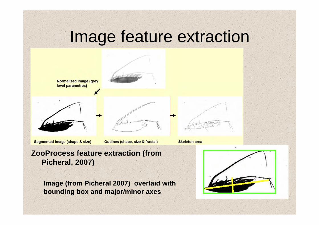
Image feature extraction
ZooProcess feature extraction (from Picheral, 2007)
Image (from Picheral 2007) overlaid with bounding box and major/minor axes

Image feature analysis
Plankton Identify (from Picheral, 2007)
• Feature sets are extracted for each object • These can then be analysed for clusters (using multi-dimensional clustering tools such as SVM, Random Forest, LDA)
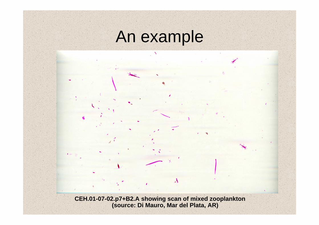
An example
CEH.01-07-02.p7+B2.A showing scan of mixed zooplankton (source: Di Mauro, Mar del Plata, AR)

An example
CEH.01-07-02.p7+B2.A showing a small sample of copepods drawn from previous slide

An example
Fig.12 Morphological data extracted automatically from CEH.01-07-02.p7+B2.A
(in Fig.11).
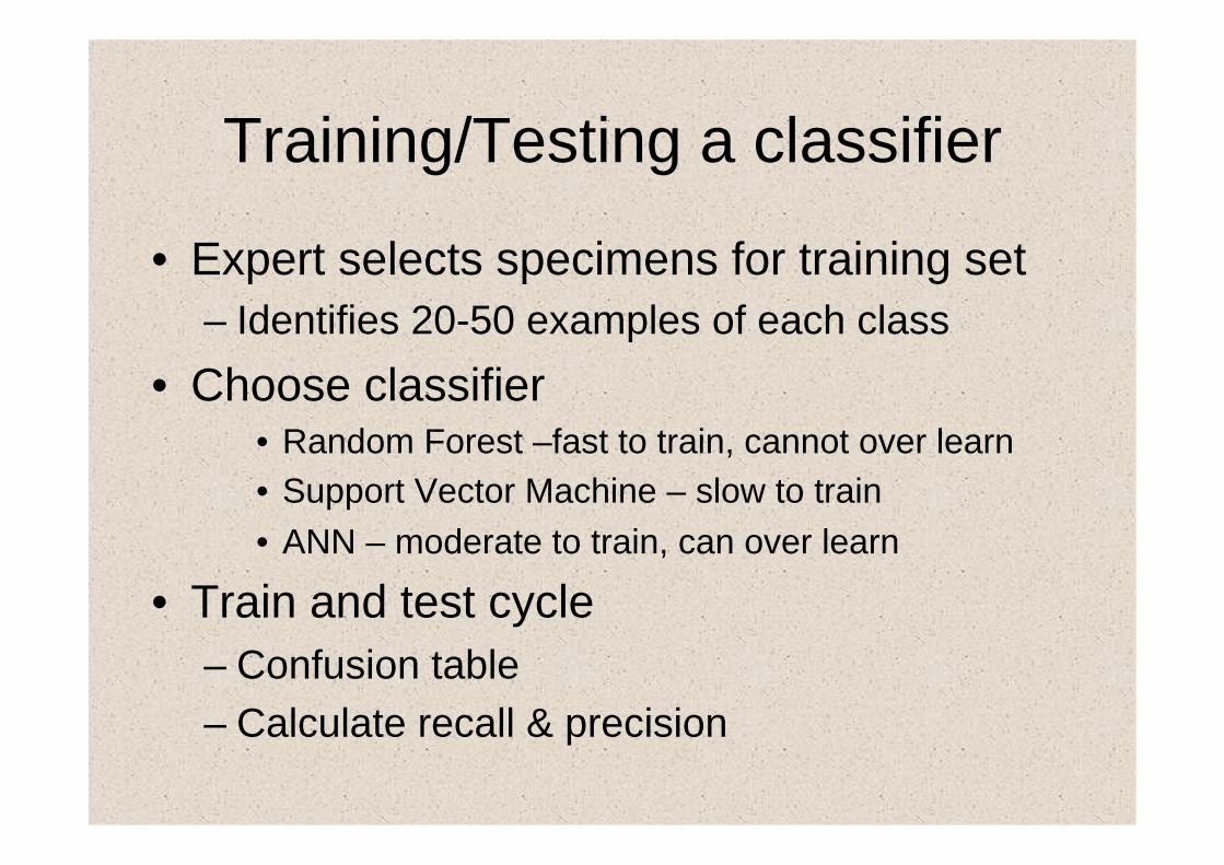
Training/Testing a classifier
• Expert selects specimens for training set – Identifies 20-50 examples of each class
• Choose classifier • Random Forest –fast to train, cannot over learn • Support Vector Machine – slow to train • ANN – moderate to train, can over learn
• Train and test cycle – Confusion table – Calculate recall & precision
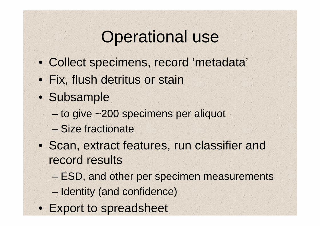
Operational use • Collect specimens, record ‘metadata’ • Fix, flush detritus or stain • Subsample
– to give ~200 specimens per aliquot – Size fractionate
• Scan, extract features, run classifier and record results – ESD, and other per specimen measurements – Identity (and confidence)
• Export to spreadsheet
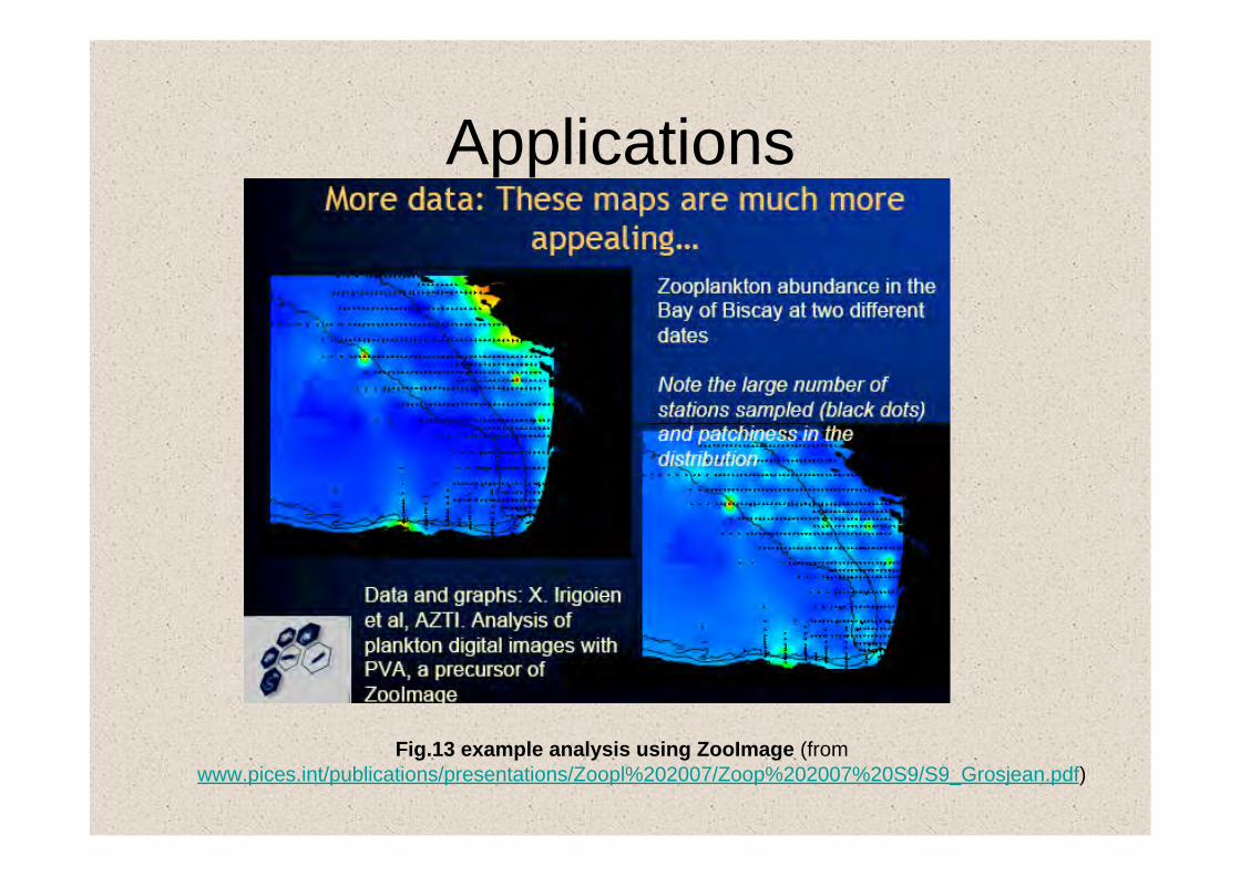
Applications
Fig.13 example analysis using ZooImage (from www.pices.int/publications/presentations/Zoopl%202007/Zoop%202007%20S9/S9_Grosjean.pdf)
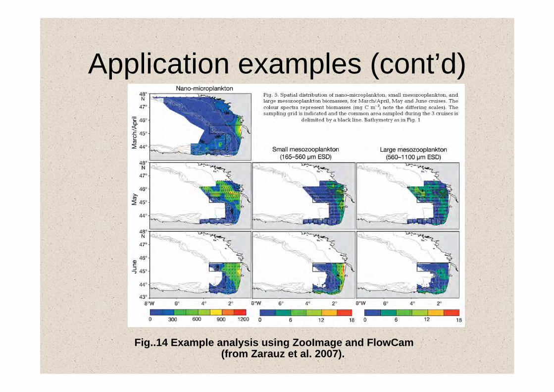
Application examples (cont’d)
Fig..14 Example analysis using ZooImage and FlowCam (from Zarauz et al. 2007).

Application examples (cont’d)
Fig.15 Example Zooscan analysis (from: Picheral 2007a)
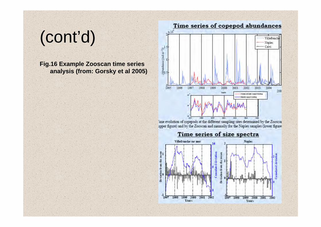
(cont’d) Fig.16 Example Zooscan time series
analysis (from: Gorsky et al 2005)

Application examples (cont’d)
Fig.17 Further examples of Zooscan time series analysis (from: Gorsky et al 2005)

Zooimage run through
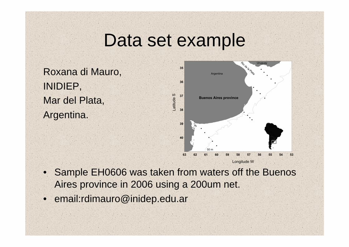
Data set example Roxana di Mauro, INIDIEP, Mar del Plata, Argentina.
• Sample EH0606 was taken from waters off the Buenos Aires province in 2006 using a 200um net.
• email:[email protected]

Machine performance
" HAB Buoy, 26 species 65-90% " Zooscan, 40 groups (semi-automatic) 75-85% " SIPPER, 5 groups 75-90% " Video Plankton Recorder,>7 groups 72% " Cytosense, 20-100 groups,
" All can process many 1,000 objects per hour
27

Conclusions for automatic visual plankton identification
• Performance OK for ecology – Flow cytometry – 60 groups – Zooscan – semiautomatic >40 groups – Zoo/Phyto Image - 20-30 groups
• Clutter and detritus can cause problems • Can make useful tools for ecology • Semi-automatic
– Keeps ecologist in the loop – Reduces false positive/negative rates

Open Forum & Discussion
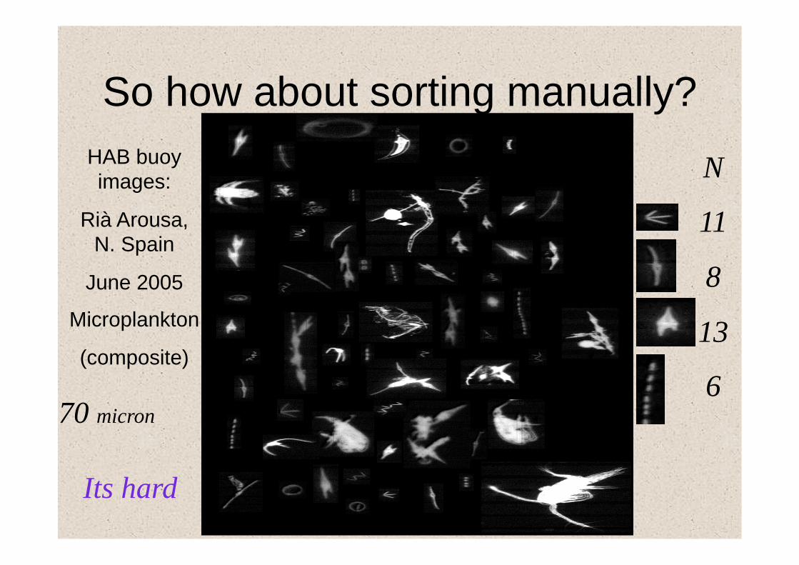
So how about sorting manually?
70 micron
N
11
8
13
6
HAB buoy images:
Rià Arousa, N. Spain
June 2005
Microplankton
(composite)
Its hard
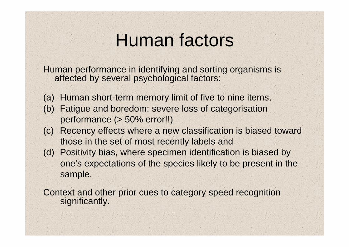
Human factors Human performance in identifying and sorting organisms is
affected by several psychological factors:
(a) Human short-term memory limit of five to nine items, (b) Fatigue and boredom: severe loss of categorisation
performance (> 50% error!!) (c) Recency effects where a new classification is biased toward
those in the set of most recently labels and (d) Positivity bias, where specimen identification is biased by
one's expectations of the species likely to be present in the sample.
Context and other prior cues to category speed recognition significantly.
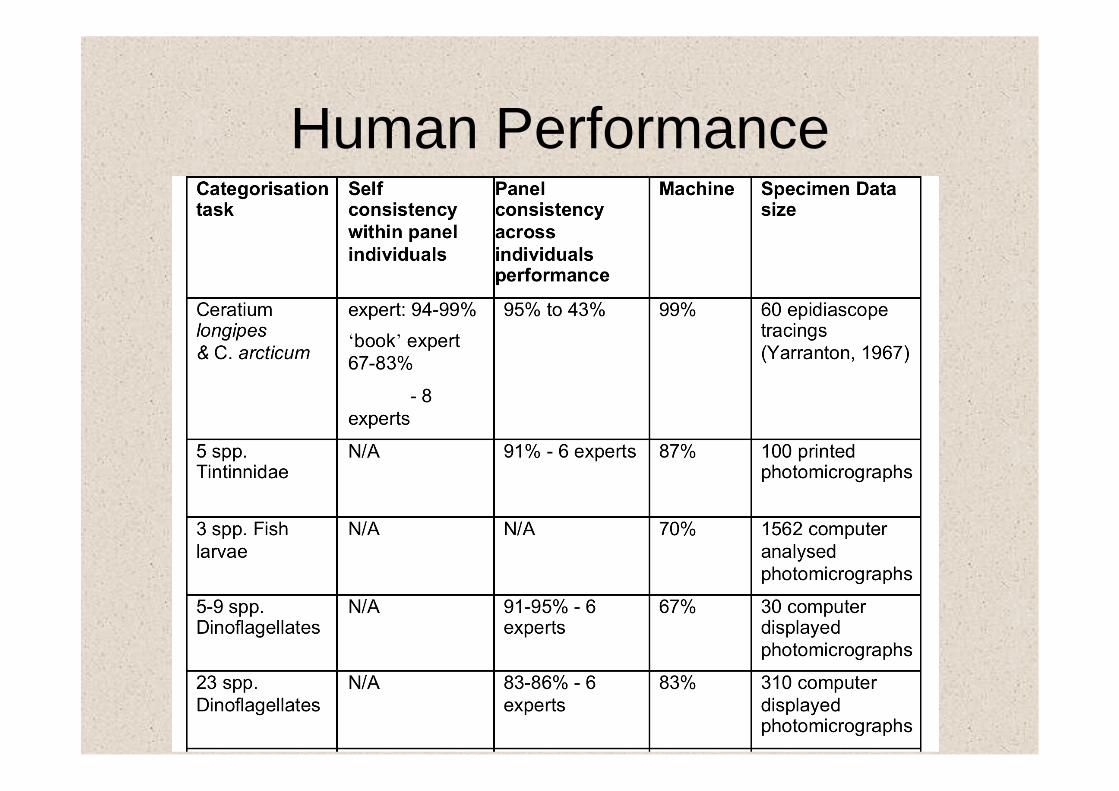
Human Performance
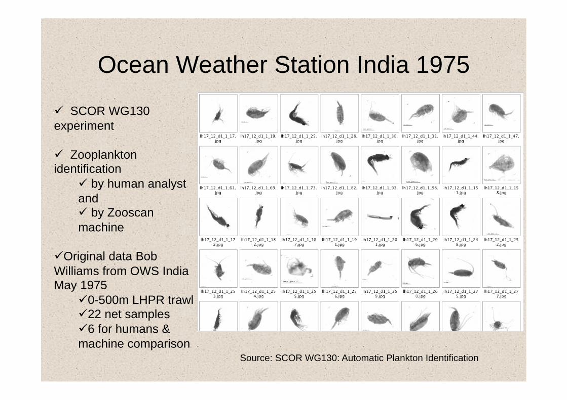
Ocean Weather Station India 1975
SCOR WG130 experiment
Zooplankton identification
by human analyst and by Zooscan machine
Original data Bob Williams from OWS India May 1975
0-500m LHPR trawl 22 net samples 6 for humans & machine comparison
Source: SCOR WG130: Automatic Plankton Identification

WS India categories
• Fixed samples in inspection trays
• Mixture of taxa and genera
• Discrimination – Some easy – Some hard
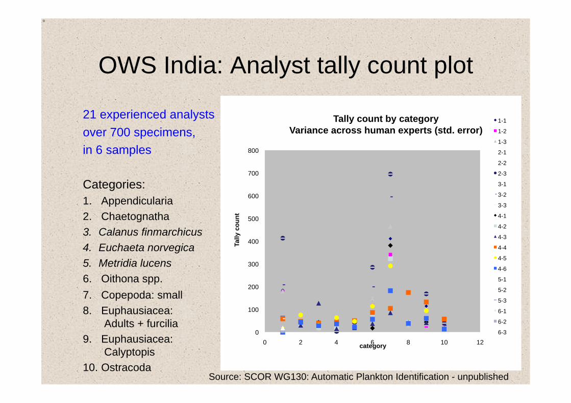
OWS India: Analyst tally count plot
21 experienced analysts over 700 specimens, in 6 samples
Categories: 1. Appendicularia 2. Chaetognatha 3. Calanus finmarchicus 4. Euchaeta norvegica 5. Metridia lucens 6. Oithona spp. 7. Copepoda: small 8. Euphausiacea:
Adults + furcilia 9. Euphausiacea:
Calyptopis 10. Ostracoda
0
100
200
300
400
500
600
700
800
0 2 4 6 8 10 12
Tally
cou
nt
category
Tally count by category Variance across human experts (std. error)
1-1
1-2
1-3
2-1
2-2
2-3
3-1
3-2
3-3
4-1
4-2
4-3
4-4
4-5
4-6
5-1
5-2
5-3
6-1
6-2
6-3
Source: SCOR WG130: Automatic Plankton Identification - unpublished

Human Performance Conclusions
– People are not perfect identification machines • Usually good at tallying (specimen counting)
15 of 21 > 90% repeatable [mean 700 specimens]
• Can be inconsistent at binning (identifying) 13 of 21 > 90% self-consistent – Experts are highly self-consistent >0.9 ICC
(Intraclass correlation coefficient) – Novices are not self-consistent 0.03 – 0.76 ICC
– Inter-analyst variation is high
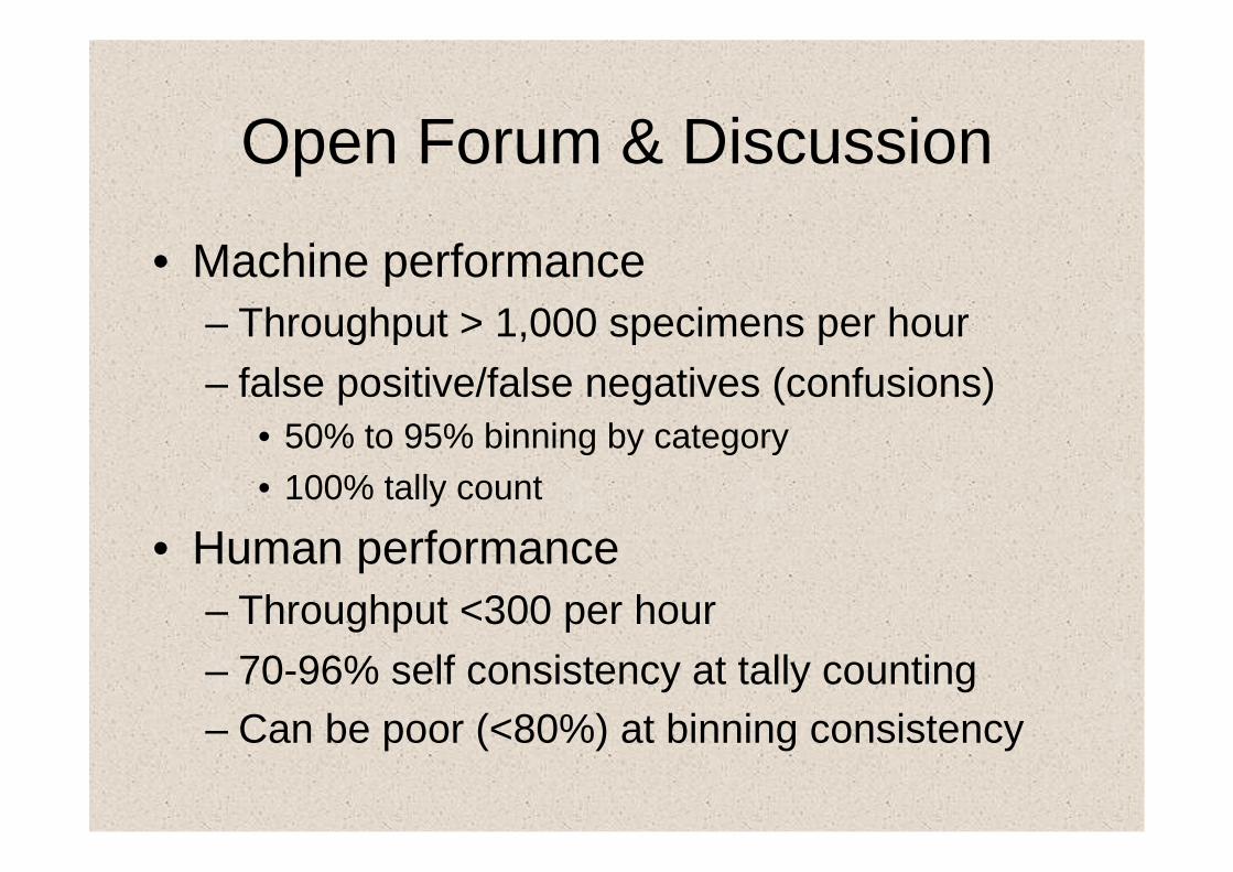
Open Forum & Discussion
• Machine performance – Throughput > 1,000 specimens per hour – false positive/false negatives (confusions)
• 50% to 95% binning by category • 100% tally count
• Human performance – Throughput <300 per hour – 70-96% self consistency at tally counting – Can be poor (<80%) at binning consistency

The Future
• Challenges include – Validating training data using scarce human
expert resources – Widespread Uptake of automation
• Funding research in this area – Cross disciplinary – Difficult for referees to review – Needs more support

Please join the RAPID group

Discuss!

References & Bibliography • Benfield MC, Grosjean P, Culverhouse PF, Irigoien X, Sieracki ME, Lopez-Urrutia A, Dam HG, Hu Q, Davis CB,
Hansen A, Pilskaln CH, Riseman E, Schultz H, Utgoff PE, and Gorsky G (2007) RAPID: Research on Automated Plankton Identification. Oceanography 20(2), pp. 12-26.
• Buskey EJ & Hyatt CJ (2006) Use of the FlowCAM for semi-automated recognition and enumeration of red tide cells (Karenia brevis) in natural plankton samples. In harmful Algae 5(6) pp.685-692
• Culverhouse, P.F., V. Herry, B. Reguera, S. González-Gil, R. Williams, S. Fonda, M. Cabrini, T. Parisini & R. Ellis (2001). Dinoflagellate Categorisation by Artificial Neural Network (DiCANN). In: Harmful Algal Blooms. Hallegraeff, G., Blackburn, S., Lewis, R. & Bolch, C. (eds.). Intergovernmental Oceanographic Commission of UNESCO, pp. 195-198.
• Culverhouse PF (2007) Natural Object Categorisation: man versus machine, in Automated Object Identification in Systematics: Theory, Approaches, and Applications - N. MacLeod (editor), Systematics Association. CRC Press. Boca Raton. US
• Davis CS, Gallager SM, Berman MS, Haury LR and Strickler.JR (1992) The Video Plankton Recorder (VPR): Design and initial results. Archiv für Hydrobiologie–Beiheft Ergebnisse der Limnologie 36:67–81.
• Gorsky G, Aldorf C, Kage M, Picheral M, Garcia Y and Favole J (1992). Vertical distribution of suspended aggregates determined by a new underwater video profiler. Annales de l’Institut Océanographique 68:275–280.
• Gorsky G, Ibanez F, Stemmann L, Grazia Mazzocchi M, Hecq JH, Warembourg C, Raybaud V (2005) Harmonization of long-term zooplankton time series in the Mediterranean. ZooPNEC group and MedZoo group related to the CIESM Task Force on Zooplankton Indicators, ASLO Summer Meeting June 19-24, Santiago de Compostela, ES.
•

References & Bibliography • Grosjean P, Picheral M, Warembourg C, & Gorsky G. (2004) Enumeration, measurement, and identification of net
zooplankton samples using the ZOOSCAN digital imaging system. ICES Journal of Marine Science 61 (4): 518. • Grosjean P & Denis K (2007) Zoo/PhytoImage version 1.2-0: Computer-Assisted Plankton Image Analysis, 25th
May 2007 from http://econum.umh.ac.be/zooimage/ZooPhytoImageManual.pdf • Picheral M (2007a) Quantitative and qualitative zooplankton data acquisition in the laboratory and in situ,
introduction to Zooscan and UVP. Presented at The Zooplankton as indicators of climate change: a bilateral cooperation between Korea and France (May 24 - 27, 2007)" held in The National Fisheries Research & Development Institute (NFRDI) at BUSAN.
• Picheral M (2007b) personal communications November 2007. • Sieracki CK, Sieracki ME and Yentsch CS. (1998) An imaging-in-flow system for automated analysis of marine
microplankton. Marine Ecology Progress Series 168:285–296. • Toth L and Culverhouse PF (1999) Three dimensional object categorisation from static 2D views using multiple
coarse channels, Image and Vision and Computing, 17 pp.845-858. • Zarauz L, Irigoien X, Urtizberea A, Gonzalez M (2007) Mapping plankton distribution in the Bay of Biscay during
three consecutive spring surveys. MEPS 345:27-39.