Embed Size (px)
Citation preview

AUTOMATIC DISCOVERY OF LATENT CLUSTERS IN GENERAL REGRESSIONMODELS
By
MINHAZUL ISLAM SK
A DISSERTATION PRESENTED TO THE GRADUATE SCHOOLOF THE UNIVERSITY OF FLORIDA IN PARTIAL FULFILLMENT
OF THE REQUIREMENTS FOR THE DEGREE OFDOCTOR OF PHILOSOPHY
UNIVERSITY OF FLORIDA
2017

© 2017 Minhazul Islam Sk

I dedicate this dissertation to my parents for their help and contributions in my life.

ACKNOWLEDGMENTS
First of all, I would like to thank all the people who have helped me in my graduate
life. I would like to thank my Ph.D. advisor Dr. Arunava Banerjee, without whom I could
not have completed my dissertation. I cannot thank him enough for his help, contribution
and motivation in my entire graduate life. I owe a lot of this journey to him as a graduate
student.
I would also like to thank my Ph.D. committee members: Dr. Anand Rangarajan, Dr.
Alireza Entezari, Dr. Malay Ghosh for their invaluable suggestions.
I would like to thank Rafael Nadal and Bernie Sanders who have inspired me in
my life with their passion, accomplishments and fight for standing up for what is right,
especially in the time of despair.
I would also like to take this opportunity to thank my entire family for helping me
to reach this stage of my life, for their financial and moral help in time of distress, for
supporting and believing in me and raising me to prepare for every adversities in my life.
4
TABLE OF CONTENTS
page
ACKNOWLEDGMENTS . . . . . . . . . . . . . . . . . . . . . . . . . . . . . . . . . . 4
LIST OF TABLES . . . . . . . . . . . . . . . . . . . . . . . . . . . . . . . . . . . . . . 8
LIST OF FIGURES . . . . . . . . . . . . . . . . . . . . . . . . . . . . . . . . . . . . . 9
ABSTRACT . . . . . . . . . . . . . . . . . . . . . . . . . . . . . . . . . . . . . . . . . 10
CHAPTER
1 INTRODUCTION . . . . . . . . . . . . . . . . . . . . . . . . . . . . . . . . . . . 12
Introduction to the Variational Inference of the DP Mixtures of GLM . . . . . . . 13Automatic Detection of Latent Common Clusters in Multigroup Regression . . . 16Automatic Discovery of Common and Idiosyncratic Effects in Multilevel Re-
gression . . . . . . . . . . . . . . . . . . . . . . . . . . . . . . . . . . . . . 19Denoising Time Series by a Flexible Model for Phase Space Reconstruction . . 22Organization of the Dissertation . . . . . . . . . . . . . . . . . . . . . . . . . . . 26
2 MATHEMATICAL BACKGROUND . . . . . . . . . . . . . . . . . . . . . . . . . 27
Generalized Linear Model . . . . . . . . . . . . . . . . . . . . . . . . . . . . . . 27Overview . . . . . . . . . . . . . . . . . . . . . . . . . . . . . . . . . . . . 27Probability Distribution . . . . . . . . . . . . . . . . . . . . . . . . . . . . . 28Linear Predictor . . . . . . . . . . . . . . . . . . . . . . . . . . . . . . . . . 28Link Function . . . . . . . . . . . . . . . . . . . . . . . . . . . . . . . . . . 28
Bayesian Statistics . . . . . . . . . . . . . . . . . . . . . . . . . . . . . . . . . . 29Bayes’ Theorem and Inference . . . . . . . . . . . . . . . . . . . . . . . . 29MAP Estimate . . . . . . . . . . . . . . . . . . . . . . . . . . . . . . . . . . 29Conjugate Prior . . . . . . . . . . . . . . . . . . . . . . . . . . . . . . . . . 29
Nonparametric Bayesian . . . . . . . . . . . . . . . . . . . . . . . . . . . . . . . 30Dirichlet Distribution and Dirichlet Process . . . . . . . . . . . . . . . . . . 30Stick Breaking Representation . . . . . . . . . . . . . . . . . . . . . . . . 31Chinese Restaurant Process . . . . . . . . . . . . . . . . . . . . . . . . . 31Dirichlet Process Mixture Model . . . . . . . . . . . . . . . . . . . . . . . . 33Hierarchical Dirichlet Process . . . . . . . . . . . . . . . . . . . . . . . . . 33Chinese Restaurant Franchise . . . . . . . . . . . . . . . . . . . . . . . . 34
3 VARIATIONAL INFERENCE FOR INFINITE MIXTURES OF GENERALIZEDLINEAR MODELS . . . . . . . . . . . . . . . . . . . . . . . . . . . . . . . . . . 37
GLM Models as Probabilistic Graphical Models . . . . . . . . . . . . . . . . . . 37Normal Model . . . . . . . . . . . . . . . . . . . . . . . . . . . . . . . . . . 37Logistic Multinomial Model . . . . . . . . . . . . . . . . . . . . . . . . . . . 37Poisson Model . . . . . . . . . . . . . . . . . . . . . . . . . . . . . . . . . 38
5

Exponential Model . . . . . . . . . . . . . . . . . . . . . . . . . . . . . . . 38Inverse Gaussian Model . . . . . . . . . . . . . . . . . . . . . . . . . . . . 39Multinomial Probit Model . . . . . . . . . . . . . . . . . . . . . . . . . . . . 40
Variational Inference . . . . . . . . . . . . . . . . . . . . . . . . . . . . . . . . . 40Variational Distribution of the Models . . . . . . . . . . . . . . . . . . . . . . . . 41
Normal Model . . . . . . . . . . . . . . . . . . . . . . . . . . . . . . . . . . 41Logistic Multinomial Model . . . . . . . . . . . . . . . . . . . . . . . . . . . 41Poisson Model . . . . . . . . . . . . . . . . . . . . . . . . . . . . . . . . . 42Exponential Model . . . . . . . . . . . . . . . . . . . . . . . . . . . . . . . 42Inverse Gaussian Model . . . . . . . . . . . . . . . . . . . . . . . . . . . . 43Multinomial Probit Model . . . . . . . . . . . . . . . . . . . . . . . . . . . . 43
Generalized Evidence Lower Bound (ELBO) . . . . . . . . . . . . . . . . . . . . 43Parameter Estimation for the Models . . . . . . . . . . . . . . . . . . . . . . . . 44
Parameter Estimation for the Normal Model . . . . . . . . . . . . . . . . . 45Parameter Estimation for the Multinomial Model . . . . . . . . . . . . . . . 47Parameter Estimation for the Poisson Model . . . . . . . . . . . . . . . . . 47Parameter Estimation for the Exponential Model . . . . . . . . . . . . . . . 48Parameter Estimation for the Inverse Gaussian Model . . . . . . . . . . . 49Parameter Estimation for the Multinomial Probit Model . . . . . . . . . . . 51
Predictive Distribution . . . . . . . . . . . . . . . . . . . . . . . . . . . . . . . . 51Experimental Results . . . . . . . . . . . . . . . . . . . . . . . . . . . . . . . . 52
Datasets . . . . . . . . . . . . . . . . . . . . . . . . . . . . . . . . . . . . . 54Timing Performance for the Normal Model . . . . . . . . . . . . . . . . . . 54Accuracy . . . . . . . . . . . . . . . . . . . . . . . . . . . . . . . . . . . . 55Tool to Understand Stock Market Dynamics . . . . . . . . . . . . . . . . . 56
4 AUTOMATIC DETECTION OF LATENT COMMON CLUSTERS OF GROUPSIN MULTIGROUP REGRESSION . . . . . . . . . . . . . . . . . . . . . . . . . . 60
Models Related to iMG-GLM . . . . . . . . . . . . . . . . . . . . . . . . . . . . 60iMG-GLM Model Formulation . . . . . . . . . . . . . . . . . . . . . . . . . . . . 60
Normal iMG-GLM-1 Model . . . . . . . . . . . . . . . . . . . . . . . . . . . 61Logistic Multinomial iMG-GLM-1 Model . . . . . . . . . . . . . . . . . . . . 62Poisson iMG-GLM-1 Model . . . . . . . . . . . . . . . . . . . . . . . . . . 62
Variational Inference . . . . . . . . . . . . . . . . . . . . . . . . . . . . . . . . . 62Normal iMG-GLM-1 Model . . . . . . . . . . . . . . . . . . . . . . . . . . . 63Logistic Multinomial iMG-GLM-1 Model . . . . . . . . . . . . . . . . . . . . 63Poisson iMG-GLM-1 Model . . . . . . . . . . . . . . . . . . . . . . . . . . 63
Parameter Estimation for Variational Distribution . . . . . . . . . . . . . . . . . 64Parameter Estimation of iMG-GLM-1 Normal Model . . . . . . . . . . . . . 64Parameter Estimation of iMG-GLM-1 Multinomial Model . . . . . . . . . . 64Parameter Estimation of Poisson iMG-GLM-1 Model . . . . . . . . . . . . 65Predictive Distribution . . . . . . . . . . . . . . . . . . . . . . . . . . . . . 65
iMG-GLM-2 Model . . . . . . . . . . . . . . . . . . . . . . . . . . . . . . . . . . 66Information Transfer from Prior Groups . . . . . . . . . . . . . . . . . . . . 66
6

Posterior Sampling . . . . . . . . . . . . . . . . . . . . . . . . . . . . . . . 67Prediction for New Group Test Samples . . . . . . . . . . . . . . . . . . . 68
Experimental Results . . . . . . . . . . . . . . . . . . . . . . . . . . . . . . . . 68Trends in Stock Market . . . . . . . . . . . . . . . . . . . . . . . . . . . . . 68Clinical Trial Problem Modeled by Poisson iMG-GLM Model . . . . . . . . 70
5 AUTOMATIC DISCOVERY OF COMMON AND IDIOSYNCRATIC LATENTEFFECTS IN MULTILEVEL REGRESSION . . . . . . . . . . . . . . . . . . . . 74
Models Related to HGLM . . . . . . . . . . . . . . . . . . . . . . . . . . . . . . 74An Illustrative Example . . . . . . . . . . . . . . . . . . . . . . . . . . . . . . . . 74iHGLM Model Formulation . . . . . . . . . . . . . . . . . . . . . . . . . . . . . . 75
Normal iHGLM Model . . . . . . . . . . . . . . . . . . . . . . . . . . . . . 75Logistic Multinomial iHGLM Model . . . . . . . . . . . . . . . . . . . . . . 76
Proof of Weak Posterior Consistency . . . . . . . . . . . . . . . . . . . . . . . . 77Gibbs Sampling . . . . . . . . . . . . . . . . . . . . . . . . . . . . . . . . . . . . 78Predictive Distribution . . . . . . . . . . . . . . . . . . . . . . . . . . . . . . . . 80Experimental Results . . . . . . . . . . . . . . . . . . . . . . . . . . . . . . . . 81
Clinical Trial Problem Modeled by Poisson iHGLM . . . . . . . . . . . . . . 81Height Imputation Problem . . . . . . . . . . . . . . . . . . . . . . . . . . . 83Market Dynamics Experiment . . . . . . . . . . . . . . . . . . . . . . . . . 84
6 SECOND PROBLEM: TIME SERIES DENOISING . . . . . . . . . . . . . . . . 87
Time Delay Embedding and False Neighborhood Method . . . . . . . . . . . . 87NPB-NR Model . . . . . . . . . . . . . . . . . . . . . . . . . . . . . . . . . . . . 88
Step One: Clustering of Phase Space . . . . . . . . . . . . . . . . . . . . 88Step Two: Nonlinear Mapping of Phase Space Points . . . . . . . . . . . . 89Step Three: Restructuring of the Dynamics . . . . . . . . . . . . . . . . . 90
Experimental Results . . . . . . . . . . . . . . . . . . . . . . . . . . . . . . . . 91An Illustrative Description of the NPB-NR Process . . . . . . . . . . . . . 91Prediction Accuracy . . . . . . . . . . . . . . . . . . . . . . . . . . . . . . 92Noise Reduction Experiment . . . . . . . . . . . . . . . . . . . . . . . . . 95Power Spectrum Experiment . . . . . . . . . . . . . . . . . . . . . . . . . 95Experiment with Dimensions . . . . . . . . . . . . . . . . . . . . . . . . . 97
7 CONCLUSION AND FUTURE WORK . . . . . . . . . . . . . . . . . . . . . . . 100
REFERENCES . . . . . . . . . . . . . . . . . . . . . . . . . . . . . . . . . . . . . . . 102
BIOGRAPHICAL SKETCH . . . . . . . . . . . . . . . . . . . . . . . . . . . . . . . . 107
7

LIST OF TABLES
Table page
3-1 Description of variational inference algorithms for the models . . . . . . . . . . 53
3-2 Run time for Gibbs sampling and variational inference . . . . . . . . . . . . . . 55
3-3 Log-likelihood of the normal model of the predictive distribution . . . . . . . . . 56
3-4 MSE and MAE of algorithms for the datasets . . . . . . . . . . . . . . . . . . . 57
3-5 List of influential stocks on individual stocks . . . . . . . . . . . . . . . . . . . . 58
4-1 Description of variational inference algorithm for iMG-GLM-1 normal model . . 66
4-2 Clusters of Stocks from Various Sectors . . . . . . . . . . . . . . . . . . . . . . 71
4-3 Mean abosulte error for all stocks for iMG-GLM-1 . . . . . . . . . . . . . . . . . 71
4-4 MSE and MAE for clinical trial and patients datasets . . . . . . . . . . . . . . . 72
5-1 Description of Gibbs sampling algorithm for iHGLM . . . . . . . . . . . . . . . . 81
5-2 List of stocks with top 3 significant stocks influencing each stock . . . . . . . . 85
5-3 MSE and MAE of the algorithms for the height imputation dataset . . . . . . . . 85
5-4 MSE and MAE of the algorithms for the clinical trial and patients datasets. . . . 86
6-1 Step-wise description of NPB-NR process. . . . . . . . . . . . . . . . . . . . . 91
6-2 Minimum embedding dimension of the attractors . . . . . . . . . . . . . . . . . 98
6-3 MSE and standard deviation of datasets for all algorithms . . . . . . . . . . . . 98
6-4 Noise reduction percentage of the attractors . . . . . . . . . . . . . . . . . . . . 99
8

LIST OF FIGURES
Figure page
2-1 Stick breaking for the Dirichlet Process . . . . . . . . . . . . . . . . . . . . . . . 32
2-2 Chinese Restaurant Process . . . . . . . . . . . . . . . . . . . . . . . . . . . . 32
2-3 Plate notation for DPMM . . . . . . . . . . . . . . . . . . . . . . . . . . . . . . . 33
2-4 Plate notation for HDPMM . . . . . . . . . . . . . . . . . . . . . . . . . . . . . . 35
2-5 Plate notation for HDPMM with indicator variables . . . . . . . . . . . . . . . . 35
2-6 Chinese Restaurant Franchise for HDP . . . . . . . . . . . . . . . . . . . . . . 36
3-1 Posterior trajectory of the normal model . . . . . . . . . . . . . . . . . . . . . . 53
3-2 Timings for synthetic datasets per dimension . . . . . . . . . . . . . . . . . . . 55
4-1 Graphical representation of iMG-GLM-1 model. . . . . . . . . . . . . . . . . . . 61
4-2 Average MAE for 51 stocks for 50 random runs for iMG-GLM-1 model . . . . . 73
4-3 Average MAE for 10 new stocks for 50 random runs for iMG-GLM-2 model . . . 73
5-1 Posterior trajectory of the synthetic dataset with 4 groups . . . . . . . . . . . . 75
5-2 Depiction of several clusters in the height imputation dataset . . . . . . . . . . 86
6-1 Plot of the noisy IBM time series data . . . . . . . . . . . . . . . . . . . . . . . 92
6-2 Depiction of noisy phase space (reconstructed). . . . . . . . . . . . . . . . . . 92
6-3 Clustered phase space and one single cluster . . . . . . . . . . . . . . . . . . . 93
6-4 Regression data: Y(1) regressed with covariate as X(1), X(2) and X(3) . . . . . 93
6-5 Single noise removed cluster and whole noise removed phase space . . . . . . 93
6-6 Plot of the noise removed time series data . . . . . . . . . . . . . . . . . . . . . 93
6-7 Power spectrum and phase space plot of attractors . . . . . . . . . . . . . . . . 96
9

Abstract of Dissertation Presented to the Graduate Schoolof the University of Florida in Partial Fulfillment of theRequirements for the Degree of Doctor of Philosophy
AUTOMATIC DISCOVERY OF LATENT CLUSTERS IN GENERAL REGRESSIONMODELS
By
Minhazul Islam Sk
August 2017
Chair: Arunava BanerjeeMajor: Computer Science
We present a flexible nonparametric Bayesian framework for automatic detection
of local clusters in general regression models. The models are built using techniques
that are now considered standard in statistical parameter estimation literature, namely
Dirichlet Process (DP), Hierarchical Dirichlet Process (HDP), Generalized Linear
Model (GLM) and Hierarchical Generalized Linear Model (HGLM). These Bayesian
nonparametric techniques have been widely applied to solve clustering problems in the
real world.
In the first part of this thesis, we formulate all traditional versions of the infinite
mixture of GLM models under the Dirichlet Process framework. We study extensively
two different inference techniques for these models, namely, variational inference and
Gibbs sampling. Finally, we evaluate their speed, and accuracy in synthetic and real
word datasets across various dimensions.
In the second part, we present a flexible nonparametric generative model for
multigroup regression that detects latent common clusters of groups. We name this
“Infinite MultiGroup Generalized Linear Model” (iMG-GLM). We present two versions
of the core model. First, in iMG-GLM-1, we demonstrate how the use of a DP prior on
the groups while modeling the response-covariate densities via GLM, allows the model
to capture latent clusters of groups by noting similar densities. The model ensures
different densities for different clusters of groups in the multigroup setting. Secondly, in
10

iMG-GLM-2, we model the posterior density of a new group using the latent densities of
the clusters inferred from previous groups as prior. This spares the model from needing
to memorize the entire data of previous groups. The posterior inference for iMG-GLM-1
is done using variational inference and that for iMG-GLM-2 using a simple Metropolis
Hastings algorithm. We demonstrate iMG-GLM’s superior accuracy in comparison to
well known competing methods like Generalized Linear Mixed Model (GLMM), Random
Forest, Linear Regression etc. on two real world problems.
In the third part, we present a flexible nonparametric generative model for multilevel
regression that strikes an automatic balance between identifying common effects
across groups while respecting their idiosyncrasies. We name it “Infinite Mixtures
of Hierarchical Generalized Linear Model” (iHGLM). We demonstrate how the use
of a HDP prior in local, group-wise GLM modeling of response-covariate densities
allows iHGLM to capture latent similarities and differences within and across groups.
We demonstrate iHGLM’s superior accuracy in comparison to well known competing
methods like Generalized Linear Mixed Model (GLMM), Regression Tree, Bayesian
Linear Regression, Ordinary Dirichlet Process regression, and several other regression
models on several synthetic and real world datasets.
For the final problem we present a framework that shows how infinite mixtures of
Linear Regression (Dirichlet Process mixtures) can be used to design a new denoising
technique in the domain of time series data that presumes a model for the uncorrupted
underlying signal rather than a model for the noise. Specifically, we show how the
nonlinear reconstruction of the underlying dynamical system by way of time delay
embedding yields a new solution for denoising where the underlying dynamics is
assumed to be highly nonlinear yet low-dimensional. The model for the underlying data
is recovered using the nonparametric Bayesian approach and is therefore very flexible.
11

CHAPTER 1INTRODUCTION
This dissertation comprises, primarily, of two parts, with nonparametric Bayesian
theories providing the central theme. The first part deals with a Bayesian nonparametric
approach to clustering of regression models in various hierarchical settings. This part
is divided into three subtopics. In the first subtopic, we outline variational inference al-
gorithms for already existing classes of infinite mixture of Generalized Linear Models. In
the second subtopic, we present a generative model framework for automatic detection
of latent common clusters of groups in multigroup regression. In the third subtopic,
we formulate a generative model for automatic discovery of common and idiosyncratic
latent effects in multilevel regression. The second part deals with a problem of denoising
time series by way of a flexible model for phase space reconstruction using variational
inference of infinite mixtures of linear regression. Each part is outlined in the following
paragraphs.
In machine learning and statistics, regression theory is a process for approximating
functional relationships among different entity/variables. This comprises of methods
for modeling relationship between multiple variables, where the first set is termed
as independent variables or predictors or covariates, while the other set is called
dependent variable or response variables. In general, regression theory evaluates the
value of expectation of the conditional distribution of the response given the covariates.
Another important parameter is the variance of the response conditional density given
the covariates. In the first part of this dissertation, we present flexible nonparametric
Bayesian frameworks for automatic detection of local clusters in general regression
models in various grouped as well as non-grouped data. In the other part, we lay out a
time series denoising technique using a dynamical system approach that uses phase
space reconstruction of the time series under consideration and then removes the noise
12
in the phase space and finally reconstructs the original noise removed time series all in
the context of Bayesian nonparametrics.
Introduction to the Variational Inference of the Dirichlet Process Mixtures ofGeneralized Linear Models
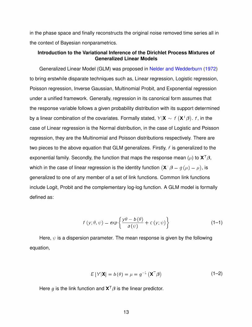
Generalized Linear Model (GLM) was proposed in Nelder and Wedderburn (1972)
to bring erstwhile disparate techniques such as, Linear regression, Logistic regression,
Poisson regression, Inverse Gaussian, Multinomial Probit, and Exponential regression
under a unified framework. Generally, regression in its canonical form assumes that
the response variable follows a given probability distribution with its support determined
by a linear combination of the covariates. Formally stated, Y |X ∼ f(XTβ). f , in the
case of Linear regression is the Normal distribution, in the case of Logistic and Poisson
regression, they are the Multinomial and Poisson distributions respectively. There are
two pieces to the above equation that GLM generalizes. Firstly, f is generalized to the
exponential family. Secondly, the function that maps the response mean (µ) to XTβ,
which in the case of linear regression is the identity function(XTβ = g (µ) = µ
), is
generalized to one of any member of a set of link functions. Common link functions
include Logit, Probit and the complementary log-log function. A GLM model is formally
defined as:
f (y ; θ,ψ) = exp
{yθ − b (θ)
a (ψ)+ c (y ;ψ)
}(1–1)
Here, ψ is a dispersion parameter. The mean response is given by the following
equation,
E [Y |X] = b (θ) = µ = g−1(XTβ)
(1–2)
Here g is the link function and XTβ is the linear predictor.
13

Notwithstanding its generality, GLM suffers from two intrinsic weaknesses, which
the authors in Hannah et al. (2011) addressed where they used the Gaussian Model.
Firstly, the covariates are associated with the model via only a linear function. Secondly,
the variance of the responses are not associated with the individual covariates. We
resolve the issues in line with Hannah et al. (2011) by introducing a mixture of GLM,
and furthermore, in order to allow the data to choose the number of clusters we impose
a Dirichlet Process prior as formulated in Ferguson (1973). Additionally, we extend the
models from just Linear and Logistic regression to all the traditional models of GLM
which we have mentioned above.
For inference, a widely applicable MCMC algorithm, namely Gibbs sampling Neal
(2000a) was employed in Hannah et al. (2011) for prediction and density estimation
using the Polya urn scheme of Dirichlet Process Blackwell and MacQueen (1973).
In spite of the generality and strength of these models, the inherent deficiencies of
Gibbs sampling significantly reduces its practical utility. As is well known, Gibbs sam-
pling approximates the original posterior distribution by sampling using a Markov chain.
However, Gibbs sampling is prohibitively slow and moreover, its convergence is very
difficult to diagnose. In high dimensional regression problems, Gibbs sampling seldom
converges to the target posterior distribution in suitable time, leading to significantly
poor density estimation and prediction Robert and Casella (2001). Although, there are
theoretical bounds on the mixing time, in practice they are not particularly useful.
To alleviate these problems, we introduce a fast and deterministic mean field
variational inference algorithm for superior prediction and density estimation of the GLM
mixtures. Variational inference is deterministic and possesses an optimization criterion
which can be used to assess convergence.
Variational methods were introduced in the context of graphical models in M. Jordan
and Saul (2001). For Bayesian applications, variational inference was employed in
Ghahramani and Beal (2000). Variational inference has found wide applications in
14

hierarchical Bayesian models such as, Latent Dirichlet Allocation D. Blei and Jordan
(2003), Dirichlet process mixtures Blei and Jordan (2006) and Hierarchical Dirichlet
Process Teh et al. (2006). To the best of our knowledge, this dissertation introduces
variational inference for the first time to nonparametric Bayesian regression.
The main contributions of this part are as follows:
• We derive the variational inference model separately for all GLM models according
to the stick breaking representation of the Dirichlet Process Sethuraman (1994).
These models differ significantly in terms of the type of covariate and response
data, which directs to markedly different variational distributions, parameter
estimation and predictive distributions. In each case, we formulate a class of
decoupled and factorized variational distributions as surrogates for the original
posterior distribution. We then maximize the lower bound (resulting from imposing
Jensen’s inequality on the log likelihood) to obtain the optimal variational parame-
ters. Finally, we derive the predictive distribution from the posterior approximation
to predict the response variable conditioned on a new covariate and the past
response-covariate pairs.
• We demonstrate the accuracy of the our variational approach across different
metrics such as, relative mean square and absolute error in high dimensional
problems against Linear regression, Bayesian and variational Linear regression,
Gaussian Process regression, and the Gibbs sampling inference in various train-
ing/testing data splits. We evaluate the log likelihood of the predictive distribution
in varying dimensions to show the superiority of variational inference against
Gibbs sampling in accuracy. Gibbs sampling fails to converge as the dimension
progressively rises.
• We experimentally show that variational inference converges substantially faster
than Gibbs sampling, thereby becoming a natural choice for practical high dimen-
sional regression problems. We show the timing performance per dimension with
15

the dimension varying from a low to a very large value for both variational and
Gibbs sampling inference in a synthetic dataset, a compiled stock market dataset,
and a disease dataset.
Introduction to Automatic Detection of Latent Common Clusters of Groups inMultiGroup Regression
Multigroup regression is the method of choice for research design whenever
response-covariate data is collected across multiple groups. When a common regressor
is learned on the amalgamated data, the resultant model fails to identify effects for
the responses specific to individual groups because the underlying assumption is that
the response-covariate pairs are drawn from a single global distribution, when the
reality might be that the groups are not statistically identical, making the joining of them
inappropriate. Modeling separate groups via separate regressors results in a model that
is devoid of common latent effects across the groups. Such a model does not exploit the
patterns common among the groups ensuring in turn the transferability of information
among groups in the regression setting. This is of particular importance when the
training set is very small for many of the groups. Joint learning, by sharing knowledge
between the statistically similar groups, strengthens the model for each group, and the
resulting generalization in the regression setting is vastly improved.
The complexities that underlie the utilization of the information transfer between
the groups are best motivated through examples. In Clinical trials, for example, a group
of people are prescribed either a new drug or a placebo to estimate the efficacy of the
drug for the treatment of a certain disease. At a population level, this efficacy may be
modeled using a single Normal or Poisson mixed model distribution with mean set as
a (linear or otherwise) function of the covariates of the individuals in the population.
A closer inspection might however disclose potential factors that explain the efficacy
results better. For example, there might be regularities at the group level—Caucasians
as a whole might react differently to the drug than, say, Asians, who might, furthermore,
16

comprise many groups. Identifying this across group information would therefore
improve the accuracy of the regressor. Similarly in the stock market, future values and
trends for a group of stocks are predicted for various sectors such as energy, materials,
consumer discretionary, financial, technology, etc. Within each sector, various stocks
share trends and therefore predicting them together (modeling them with the same time
series via autoregressive density) is usually much more accurate than predicting and
capturing individual trends. Modeling the latent common clustering effects of cross-
cutting subgroups is therefore an important problem to solve. We present a framework
here that accomplishes this.
For multigroup regression, Generalized Linear Mixed Model (GLMM) Breslow and
Clayton (1993) and Hierarchical Generalized Linear Mixed Model Lee and Nelder (1996)
have been developed where similarities between groups is captured though a fixed
effect and variation across groups is captured through random effects. Statistically,
these models are very rigid since every group is forced to manifest the same fixed
effect, while the random effect only represents the intercept parameter of the linear
predictors. Cluster of groups may have significantly different properties from other
clusters of groups, a feature that is not captured in these traditional GLM based models.
Furthermore, various clusters of groups may have different uncertainties with respect to
the covariates which we denote as heteroscedasticity. In recent progress, Bakker and
Heskes (2003) has proposed a Bayesian hierarchical model, where a prior is used for
the mixture of groups. Nevertheless, individual groups are given weights as opposed to
jointly learning various groups. Also, the number of mixtures are fixed in advance.
Before, presenting our algorithm, we describe our basis for identifying group-
correlation. First, two groups are correlated if their responses follow the same distri-
bution. Second, two groups that have the same response variance with respect to the
covariates are deemed to be correlated. This is achieved via a Dirichlet Process prior
17
on the groups and the covariate coefficients (β). The posterior is obtained by appropri-
ately combining the prior and the data likelihood from the given groups. The prior helps
cluster the groups and the likelihood from the individual groups help in the sharing of
trends between groups to create the single posterior density between the many potential
groups, thereby leading to group-correlation.
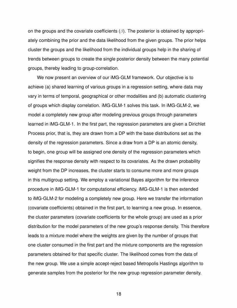
We now present an overview of our iMG-GLM framework. Our objective is to
achieve (a) shared learning of various groups in a regression setting, where data may
vary in terms of temporal, geographical or other modalities and (b) automatic clustering
of groups which display correlation. iMG-GLM-1 solves this task. In iMG-GLM-2, we
model a completely new group after modeling previous groups through parameters
learned in iMG-GLM-1. In the first part, the regression parameters are given a Dirichlet
Process prior, that is, they are drawn from a DP with the base distributions set as the
density of the regression parameters. Since a draw from a DP is an atomic density,
to begin, one group will be assigned one density of the regression parameters which
signifies the response density with respect to its covariates. As the drawn probability
weight from the DP increases, the cluster starts to consume more and more groups
in this multigroup setting. We employ a variational Bayes algorithm for the inference
procedure in iMG-GLM-1 for computational efficiency. iMG-GLM-1 is then extended
to iMG-GLM-2 for modeling a completely new group. Here we transfer the information
(covariate coefficients) obtained in the first part, to learning a new group. In essence,
the cluster parameters (covariate coefficients for the whole group) are used as a prior
distribution for the model parameters of the new group’s response density. This therefore
leads to a mixture model where the weights are given by the number of groups that
one cluster consumed in the first part and the mixture components are the regression
parameters obtained for that specific cluster. The likelihood comes from the data of
the new group. We use a simple accept-reject based Metropolis Hastings algorithm to
generate samples from the posterior for the new group regression parameter density.
18

For both iMG-GLM-1 and iMG-GLM-2, we use Monte Carlo integration for evaluating the
predictive density of the new test samples.
We evaluate both iMG-GLM-1 and iMG-GLM-2 Normal models in two real world
problems. The first is the prediction and finding of trends in the stock market. We
show how information transfer between groups help our model to effectively predict
future stock values by varying the number of training samples in both previous and new
groups. In the second, we show the efficacy of i-MG-GLM-1 and i-MG-GLM-2 Poisson
model against its competitors in a very important clinical trial problem setting.
Introduction to Automatic Discovery of Common and Idiosyncratic Latent Effectsin Multilevel Regression
Hierarchical Generalized Linear Model (HGLM), proposed in Lee and Nelder (1996),
extends GLM to already grouped observations. Hierarchical Generalized Linear Model is
formally defined as:
f (y ; θ,ψ, u) = exp
{yθ − b (θ)
a (ψ)+ c (y ;ψ)
}(1–3)
Here, ψ is a dispersion parameter and u is the random effect component. The mean
response is E [Y |X] = b (θ) = µ = g−1(XTβ + v
), where g is the link function, XTβ
is the linear predictor and v is a strictly monotonic function of u,{v = v (u)}. Here, v
signifies over-dispersion. u has a prior distribution chosen appropriately.
Therefore, in HGLM, the separate densities are characterized by two main com-
ponents. First, there is a fixed effect parameter,(XTβ
)of the density which includes
the covariates X and its coefficients (β). They are same for all the groups. Secondly,
there is a random effect part (v ) which is different in different groups. Notwithstanding
its generality and effectiveness, the inherent assumptions in HGLM limit its performance
and need to be relaxed.
Firstly, the random effect (u) is not a function of the linear transformation of the
covariates, XTβ. Therefore, this automatically assumes that the mean function and the
19

variance of the outcomes in different groups depend neither on the covariate, X , nor on
the coefficients. This makes the model suitable only for grouped data where properties
of the outcomes in different groups vary independently of covariates. Secondly, although
the response-covariate pairs are grouped, two different pairs in the same group may
come from different response-covariate densities. Likewise, any two pairs from two
different groups may be generated from the same density. Therefore, we need a
robust model that captures this hidden intra/inter clustering effect in already grouped
data. Thirdly, the covariate (XTβ) is associated with the response-covariate density
only through a linear function. Although we can introduce a non-linear function for
the response at the output, it does not include the covariates. Finally, data may be
heteroscedastic within the individual group also, i.e. the variance of the response may
be a function of the predictors within each groups. The response variance however
does not depend on the predictors in ordinary HGLM. Some later version Lee and
Nelder (2001a) of HGLM picks heteroscedasticity between the groups (different variance
for different groups), but within specific groups response variance does not vary with
covariates.
Many examples of the kind of problem that motivates us can be found in Clinical
trials, tree height imputation and in other areas. In clinical trialsIBM (2011), a group of
people are given either a new drug or a placebo to estimate the effect of the new drug
for treatment of a certain disease. Normally, these are modeled by Normal or Poisson
Mixed model, which predicts the effectiveness of the new drug. In practice, it has been
found that different people react differently to new drugs. Also, persons in different
groups can behave similarly to the new drug. Therefore, prediction of usefulness of
the new drugs as a whole is not perfect. Also, the variability of the reaction must be
different among people within groups and different groups and they must depend on
the covariates such as, treatment center size, gender, age etc. In height imputation
Robinson and Wykoff (2004) for forest stands, heights are generally regressed with
20

various tree attributes like tree diameter, past increments etc., which gives a projection
for forest development under various management strategies. These are modeled by
traditional Normal GLMM where the free coefficient(β0) becomes the random effect. The
underlying assumption is that trees in one stand have the same growth properties while
having completely different growth properties in different stands, which is not true. We
need a robust enough model to capture these shared growth properties among stands
for proper projection of overall forest development. Also, the model should pick up the
variance in growth measurements w.r.t. the diameters, past increments and other tree
attributes across stands.
In this dissertation, we alleviate these assumptions of HGLM by developing iHGLM,
a Non-parametric Bayesian Mixture Model of the Hierarchical Generalized linear Model.
The iHGLM framework is specified to all the models of HGLM, i.e. Normal, Poisson,
Logistic, Inverse Gaussian, Probit, Exponential etc.
In iHGLM, we model outcomes in the same group via mixtures of local densities.
This captures locally similar regression patterns, where each local regression is ef-
fectively a GLM. To force the density of the covariate, X , and its coefficients, β, to be
shared among groups, we make the coefficients, β, and the covariates, X , for different
groups be generated from the same prior atomic distribution. An atomic distribution
places finite probabilities on a few outcomes of the sample space. When the coeffi-
cients, β, and the covariates, X , are drawn from this atomic density, it enables the X and
β in different groups to share densities. In this way, in the Bayesian setting, along with
the density of random effect (u), the density of fixed effect (XTβ) is also shared among
groups. We obtain this prior atomic density for fixed and random effect, while ensuring
a large support, through a Hierarchical Dirichlet Process (HDP) priorY. W. Teh and Blei
(2006).
From the HDP prior, our main goal is to generate prior densities of fixed effect u
and (XTβ) for each group. We draw a density G0 from a Dirichlet Process (DP(γ,H))
21

Ferguson (1973). In this case, the H (the base distribution) is basically the set of
densities in the parameter space of fixed (u) and random effect (XTβ). According
to Sethuraman (1994), this ensures that G0 is atomic, yet having a broad support.
Therefore, G0 is an atomic density in the parameter space of u and (XTβ) which puts
finite probabilities on several discrete points which acts as its support. Then, for each
group, we draw group specific densities Gj from DP(α,G0). Since G0 is already atomic,
and therefore according to Sethuraman (1994), Gj is also atomic and hence the support
of group specific densities Gjs must share common points in their respective parameter
space of fixed (u) and random (XTβ) effect. Now, this Gj acts as prior densities for the u
and XTβ for each group. Subsequently, both u and XTβ are modeled through mixture of
local densities which are shared among groups.
For each component (clusters within groups) in the mixture of response-covariate
densities in a single group, although the mean function is linear, marginalizing out
the local distribution creates a non-linear mean function. In addition, the variance of
the responses vary among mixture components (clusters), thereby varying among
covariates. The non-parametric model ensures that the data would determine the
number of mixture components (clusters) in specific groups and the nature of the local
GLMs.
Introduction to Denoising Time Series by Way of a Flexible Model for Phase SpaceReconstruction
In this part, we outline a technique for denoising a time series by way of a flexible
model for phase space reconstruction. Noise is a high dimensional dynamical system
which limits the extraction of quantitative information from experimental time series
data. Successful removal of noise from time series data requires a model either for the
noise or for the dynamics of the uncorrupted time series. For example, in wavelet based
denoising methods for time series Mallat and Hwang (1992); Site and Ramakrishnan
(2000), the model for the signal assumes that the expected output of a forward/inverse
22

wavelet transform of the uncorrupted time series is sparse in the wavelet coefficients.
In other words, it is presupposed that the signal energy is concentrated on a small
number of wavelet basis elements; the remaining elements with negligible coefficients
are considered noise. Hard-threshold wavelet Zhang et al. (2001) and Soft-threshold
wavelet David and Donoho (1995) are two widely known noise reduction methods that
subscribe to this model. Principal Component Analysis, on the other hand, assumes a
model for the noise: the variance captured by the least important principal components.
Therefore, denoising is accomplished by dropping the bottom principal components and
projecting the data onto the remaining components.
In many cases, the time series is produced by a low-dimensional dynamical system.
In such cases, the contamination of noise in the time series can disable measurements
of the underlying embedding dimension Kostelich and Yorke (1990), introduce extra
Lyapunov Exponents Badii et al. (1988), obscure the fractal structure Grassberger et al.
(1991) and limit prediction accuracy Elshorbagy and Panu (2002). Therefore, reduction
of noise while maintaining the underlying dynamics generated from the time series is of
paramount importance.
A widely used method in time series denoising is Low-pass filtering. Here noise
is assumed to constitute all high frequency components without reference to the
characteristics of the underlying dynamics. Unfortunately, low pass filtering is not well
suited to non-linear chaotic time series Wang et al. (2007). Since the power spectrum of
low-dimensional chaos resembles a noisy time series, removal of the higher frequencies
distorts the underlying dynamics, thereby, adding fractal dimensions Mitschke et al.
(1988).
In this dissertation, we present a phase space reconstruction based approach to
time series denoising. The method is founded on Taken’s Embedding Theorem Takens
(1981), according to which a dynamical system can be reconstructed from a sequence
of observations of the output of the system (considered, here, the time series). This
23

respects all properties of the dynamical system that do not change under smooth
coordinate transformations.
Informally stated, the proposed technique can be described as follows: Consider
a time series, x(1), x(2), x(3)..... corrupted by noise. We first reconstruct the phase
space by taking time delayed observations from the noisy time series (for example,
⟨x(i), x(i + 1)⟩ forms a phase space trajectory in 2-dimensions). The minimum embed-
ding dimension (i.e., number of lags) of the underlying phase space is determined via
the False Neighborhood method Kennel et al. (1992). Next, we cluster the phase space
without imposing any constraints on the number of clusters. Finally, we apply a nonlinear
regression to approximate the temporally subsequent phase space points for each point
in each cluster via a nonparametric Bayesian approach. Henceforth, we refer to our
technique by the acronym NPB-NR, standing for nonparametric Bayesian approach to
noise reduction in Time Series.
To elaborate, the second step clusters the reconstructed phase space of the time
series through an Infinite Mixture of Gaussian distribution via Dirichlet Process Ferguson
(1973). We consider the entire phase space to be generated from a Dirichlet Process
mixture (DP) of some underlying density Escobar and West (1995). DP allows the
phase space to choose as many clusters as fits its dynamics. The clusters pick out small
neighborhoods of the phase space where the subsequent non-linear approximation
would be performed. As the latent underlying density of the phase space is unknown,
modeling this with an Infinite mixture model allows NPB-NR to correctly find the phase
space density. This is because of the guarantee of posterior consistency of the Dirichlet
Process Mixtures under Gaussian base densityS. Ghosal and Ramamoorthi (1999).
Therefore, we choose the mixing density to be Gaussian. The posterior consistency acts
as a frequentist justification of Bayesian methods—as more data arrives, the posterior
density concentrates on the true underlying density of the data.
24

In the third step, our goal is to non-linearly approximate the dynamics in each clus-
ter formed above. We use a DP mixture of Linear regression to non-linearly map each
point in a cluster to its image (the temporally subsequent point in the phase space). In
this infinite mixtures of regression, we model the data in a specific cluster via a mixtures
of local densities (Normal density with linear combination of the covariates (βX ) as the
Mean). Although the mean function is linear for each local density, marginalizing over
the local distribution creates a non-linear mean function. In addition, the variance of
the responses vary among mixture components in the clusters, thereby varying among
covariates. The nonparametric model ensures that the data determines the number of
mixture components in specific clusters and the nature of the local regressions. Again,
the basis for the infinite mixture model of linear regression is the guarantee of posterior
consistency Tokdar (2006).
In the final step, we restructure the dynamics by minimizing the sum of the deviation
between each point in the cluster and its pre-image (previous temporal point) and
post-image (next temporal point) yielded by the non-linear regression described above.
To create a noise removed time series out of the phase space, readjustment of the
trajectory is done by maintaining the co-ordinates of the phase space points to be
consistent with time delay embedding.
We demonstrate the accuracy of the NPB-NR model across several experimental
settings such as, noise reduction percentage and power spectrum analysis on several
dynamical systems like Lorenz, Van-der-poll, Buckling Column, GOPY, Rayleigh and
Sinusoid attractors, as compared to low pass filtering. We also show the forecasting
performance of the NPB-NR method in time series datasets from various domain like
the “DOW 30” index stocks, LASER dataset, Computer Generated Series, Astrophysical
dataset, Currency Exchange dataset, US Industrial Production Indices dataset, Darwin
Sea Level Pressure dataset and Oxygen Isotope dataset against some of its competitors
like GARCH, AR, ARMA, ARIMA, PCA, Kernel PCA and Gaussian Process regression.
25

Organization of the Dissertation
In chapter 2, we briefly describe Generalized Linear Models and Bayesian inference
theory, with focus on the nonparametric Bayesian framework and its various represen-
tations. In Chapter 3, we outline the variational inference of Dirichlet Process mixtures
of Generalized Linear Models. Chapter 4 presents the clustering models for multigroup
regression. Chapter 5 outlines the automatic detection of latent Common and idiosyn-
cratic effects in multilevel regression. Finally, in Chapter 6, we present the time series
denoising method in details. Chapter 7 discusses future directions.
26
CHAPTER 2MATHEMATICAL BACKGROUND
Generalized Linear Model
Overview
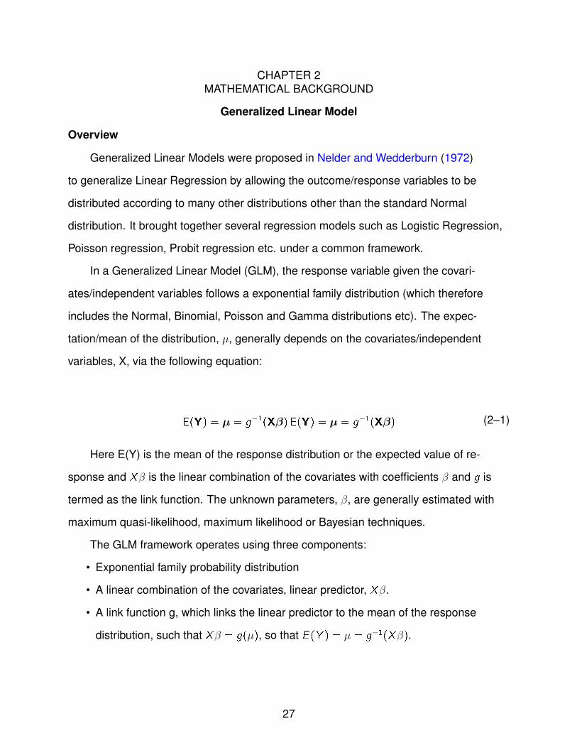
Generalized Linear Models were proposed in Nelder and Wedderburn (1972)
to generalize Linear Regression by allowing the outcome/response variables to be
distributed according to many other distributions other than the standard Normal
distribution. It brought together several regression models such as Logistic Regression,
Poisson regression, Probit regression etc. under a common framework.
In a Generalized Linear Model (GLM), the response variable given the covari-
ates/independent variables follows a exponential family distribution (which therefore
includes the Normal, Binomial, Poisson and Gamma distributions etc). The expec-
tation/mean of the distribution, µ, generally depends on the covariates/independent
variables, X, via the following equation:
E(Y) = µ = g−1(Xβ) E(Y) = µ = g−1(Xβ) (2–1)
Here E(Y) is the mean of the response distribution or the expected value of re-
sponse and Xβ is the linear combination of the covariates with coefficients β and g is
termed as the link function. The unknown parameters, β, are generally estimated with
maximum quasi-likelihood, maximum likelihood or Bayesian techniques.
The GLM framework operates using three components:
• Exponential family probability distribution
• A linear combination of the covariates, linear predictor, Xβ.
• A link function g, which links the linear predictor to the mean of the response
distribution, such that Xβ = g(µ), so that E(Y ) = µ = g−1(Xβ).
27

Probability Distribution
A GLM model is therefore formally defined in terms of probability distribution as:
f (y ; θ,ψ) = exp
{yθ − b (θ)
a (ψ)+ c (y ;ψ)
}(2–2)
Here, ψ is a dispersion parameter. There are many common distributions that
belong to this exponential family. They are Normal, Gamma, Beta, Dirichlet, Multinomial
etc.
Linear Predictor
The linear predictor is the linear combination of the independent variables, X . This
is the entity that gathers the information about the independent variables and then
includes them in the model. This is also tightly related to the link function which we
describe in the next section
η = Xβ.
Link Function
The link function links the expectation/mean of the response distribution to the
linear predictor. So, the linear predictor goes into the model via this function which
is the response of the distribution. There are many commonly used link functions in
Generalized Linear Model family. For Normal model, Xβ = µ, the identity link function.
For Exponential and Gamma model, it is the inverse link, Xβ = µ−1. For Inverse
Gaussian model, the link function is the inverse squared, Xβ = µ−2. For Poisson model,
the link function is the log link, Xβ = ln(µ). For Bernoulli, Categorical/Multinomial Model,
it is the Logit function, ln( µ1−µ
).
28
Bayesian Statistics
Bayes’ Theorem and Inference
Bayesian inference is a manner of doing statistical inference where we use Bayes’
theorem to calculate the the probability for an unknown quantity as we gather more and
more information. There is a prior distribution P(θ|β) for the unknown quantity θ, (here, β
is the hyper parameter) and the observed data (X1,X2, ......)is modeled to be distributed
independently and identically (i.i.d.) according to a distribution P(X |θ). Now, given this
data, according to Bayes’ rule, the posterior distribution of θ is given by
P(θ|X, β) = P(X|θ)P(θ|β)P(X|β)
=P(X|θ)P(θ|β)∫
θP(X|θ)P(θ|β)dθ (2–3)
Here, P(X |β) is known as the marginal likelihood.
MAP Estimate
MAP estimate is the mode (optima) of the posterior distribution. This is nothing
but a point estimate of the unknown parameter based on the observed data. This is
accomplished by optimizing the posterior with respect to the unknown parameter θ. This
is given by,
θMAP = argmaxθ
P(θ|X, β) (2–4)
This is easy to evaluate when the posterior has a closed form known distribution,
which brings the idea of conjugate prior.
Conjugate Prior
When the posterior distribution, p(θ|X , β) has the same analytical from as the prior
distribution p(θ|β), they are termed as conjugate to each other. In that case, the prior
becomes a conjugate prior for that likelihood p(X |θ). This is an algebraic convenience
where the posterior distribution can be determined in a closed form. For example,
29

the Gaussian distribution is conjugate to another Gaussian (where only the mean is
unknown), Dirichlet distribution is conjugate for Multinomial likelihood, Beta density is the
conjugate for Binomial likelihood. Every exponential family distribution has a conjugate
prior.
Nonparametric Bayesian
The analytical form of the data distribution is assumed in parametric Bayesian
theory. This is very limiting in the sense that the number of parameters in the model
does not depend on the data, rather this is pre-fixed. But, in nonparametric Bayesian
statistics, the parameter space is infinite-dimensional. As the model obtains more and
more data, it automatically evaluates the status of the existing parameters or adds more
parameters to suitably reflect the data. Nonparametric Bayesian statistics have been
studied extensively in machine learning in the domain of classification, regression,
financial markets, time series prediction, dynamical systems etc.
Dirichlet Distribution and Dirichlet Process
The Dirichlet distribution is a multivariate version of the Beta distribution. It is
defined on the K-dimensional simplex. If, x = (x1, x2, , , xK) represents a K-dimensional
probability space, such that ∀i , xi ≥ 0and∑K
k=1 xk = 1, then the Dirichlet distribution is
given by,
Dir(x1, , , , xK |α1,α2, , , ,αK) =�(∑K
k=1 αk)
��(αk)�Kk=1x
αk−1k
(2–5)
Here, E [xk ] = αk∑Kk=1 αk
, Var [xk ] =αk(αk−
∑Kk=1 αk)
(∑K
k=1 αk))2(∑K
k=1 αk)+1)
The Dirichlet distribution is the conjugate prior to the categorical and multinomial
distribution. Therefore, when the data likelihood follows a categorical/multinomial
distribution, the prior should be a Dirichlet distribution to get a Dirichlet distribution as
the posterior.
30

A Dirichlet Process Ferguson (1973), D (α0,G0) is defined as a probability measure
over (X ,B(X )), such that for any finite partition of X = A1 ∪ A2 ∪ A3... ∪ AK .
(G(A1),G(A2), ...,G(AN)) ∼ Dir(α0A1,α0A2, ...,α0AK) (2–6)
D (α0,G0) is defined as a probability distribution on a sample space of probability
distribution. Here, α0 is the concentration parameter and G0 is the base distribution.
Here, E [G(A)] = G0(A) and V [G(A)] = G0(A)(1 − G0(A))/(α0 + 1), where, A is any
subset of X belonging to its sigma algebra.
There are two well known representations of Dirichlet Process which we would
describe below.
Stick Breaking Representation
According to the stick-breaking construction Sethuraman (1994) of DP, G , which is a
sample from DP, is an atomic distribution with countably infinite atoms drawn from G0.
βi |α0,G0 ∼ Beta(1,α0), θi |α0,G0 ∼ G0
πi = vi
i−1∏l=1
(1− vl) , G =
∞∑i=1
πi .δθi
(2–7)
Chinese Restaurant Process
A second representation of the Dirichlet process is given by the Polya urn Process
Blackwell and MacQueen (1973). This clearly proves the clustering property of the
Dirichlet Process. Let θ1, θ2, ... be independent and identically distributed draws from G .
Then the conditional distribution θn|θ1, θ2, ..........θn−1 is given by,
θn|θ1, θ2θ3θn−1,α0,G0 ∼n−1∑i=1
1
n − 1 + α0δθi +
α0n − 1 + α0
G0 (2–8)
31

Figure 2-1. Stick Breaking for the Dirichlet Process
Figure 2-2. Chinese Restaurant Process
Basically, an atom, θ would be drawn with more probability if the atom has been
drawn before. Each time a new atom may be drawn with probability α0.
32

Figure 2-3. Plate notation for DPMM
Dirichlet Process Mixture Model
In the DP mixture model Antoniak (1974), Escobar and West (1995), DP is used as
a nonparametric prior over parameters of an infinite mixture model Ishwaran and James
(2001).
zn| {v1, v2, ...} ∼ Categorical {π1,π2,π3....}
Xn|zn, (θi)∞i=1 ∼ F (θzn)
(2–9)
Here, F is a distribution parametrized by θzn .
Hierarchical Dirichlet Process
Hierarchical Dirichlet Process was proposed in Y. W. Teh and Blei (2006) to model
grouped data. Here, an individual group is modeled according to a mixture model. A
Hierarchical Dirichlet Process is defined as a distribution over a set of random probability
measures. There is a random probability measure Gj for each group and a universal
33

random probability measure G0. The universal measure G0 is a draw from a Dirichlet
process parametrized by concentration parameter γ and base probability measure H.
G0|γ,H ∼ DP(γ,H) (2–10)
Now, each Gj is a draw from a DP parametrized by α0 and G0.
Gj |α0,G0 ∼ DP(α0,G0) (2–11)
The HDP Mixture model is given by,
θj ,i |Gj ∼ Gj
xj ,i |θj ,i ∼ F (θj ,i)
(2–12)
Here, θj ,i is the latent parameter for i th element in the j th group and xj ,i is the i th
element in the j th group. Now that, G0 is a draw from a DP, this forms an atomic distri-
bution according to the previous section. When Gjs are drawn, they invariably share
some of those atoms because they all are drawn from the same G0. Therefore, Hierar-
chical Dirichlet Process has this unique capability of picking shared latent parameters in
grouped data in an infinite mixture model setting.
Chinese Restaurant Franchise
In the Chinese Restaurant Franchise (CRF), we have a finite number of restaurants
(groups) with infinite number of tables (clusters) with shared dishes (parameter) among
all restaurants. Let θji be the customers, ϕ1:K be the global dishes, jt be the table-
specific dishes, tji be the table index of j th restaurant (jt) and i th customer (θji ), kjt be
the table menu index of the j th restaurant (jt) and tth table (ϕk ). Again, njt· and nj ·k
denotes the number of customers in the tth table-j th restaurant and j th restaurant-k th
34

Figure 2-4. Plate notation for HDPMM
Figure 2-5. Plate notation for HDPMM with indicator variables
35
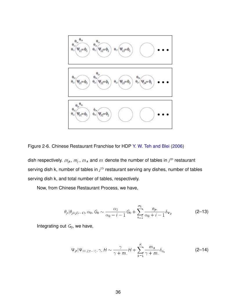
Figure 2-6. Chinese Restaurant Franchise for HDP Y. W. Teh and Blei (2006)
dish respectively. mjk , mj ·, m·k and m· denote the number of tables in j th restaurant
serving dish k, number of tables in j th restaurant serving any dishes, number of tables
serving dish k, and total number of tables, respectively.
Now, from Chinese Restaurant Process, we have,
θji |θj1:j(i−1),α0,G0 ∼α0
α0 + i − 1G0 +
mj·∑t=1
njt·
α0 + i − 1δjt
(2–13)
Integrating out G0, we have,
jt |11:j(t−1), γ,H ∼ γ
γ +m··H +
K∑k=1
m·k
γ +m··δϕk (2–14)
36

CHAPTER 3VARIATIONAL INFERENCE FOR INFINITE MIXTURES OF GENERALIZED LINEAR
MODELS
GLM Models as Probabilistic Graphical Models
We begin by assuming the continuous covariate-response pairs in the models as a
probabilistic graphical model according to its stick breaking representation. The Normal
and Multinomial Model was presented in Hannah et al. (2011), we extend to the other
models.
Normal Model
In Normal Model, the generative model of the covariate-response pair is given by
the following set of equations.
vi |α1,α2 ∼ Beta(α1,α2)
{µi ,d ,λx ,i ,d} ∼ N(µi ,d |mx ,d , (βx ,d ,λx ,i ,d)
−1)
Gamma (λx ,i ,d |ax ,d , bx ,d)
{βi ,d ,λy ,i} ∼ N(βi ,d |my ,d , (βy ,λy ,i)
−1)
Gamma (λy ,i |ay , by)
zn| {v1, v2, .....} ∼ Categorical {M1,M2,M3....}
Xn|zn ∼ N (µzn,d ,λx ,zn,d)
Yn|Xn, zn ∼ N
(βzn,0 +
D∑d=1
βzn,dXn,d ,λ−1y ,zn
)
(3–1)
Here, Xn and Yn represents the continuous response-covariate pairs. {z , v , ηx , ηy} is
the set of latent variables and the distributions, {µi ,d ,λx ,i ,d} and {βi ,d ,λy ,i} are the base
distributions of the DP.
Logistic Multinomial Model
In the logistic multinomial model, the continuous covariates are modeled by a
Gaussian mixture and a multinomial logistic framework is used for the categorical
37

response. In this model, the covariate and zn are modeled identically as the Normal
Model above. Hence, we present only the response distribution.
{βi ,d} ∼ N(βi ,d |my ,d ,k , s
2y ,d ,k
)Yn|Xn, zn ∼
exp(βzn,0,k +
∑D
d=1 βzn,d ,kXn,d
)∑K
k=1 exp(βzn,0,k +
∑D
d=1 βzn,d ,kXn,d
) (3–2)
Here, {z , v , ηx , ηy} are the latent variables and {µi ,d ,λx ,i ,d} and {βi ,d} are the DP
base distributions.
Poisson Model
In the Poisson Model, the categorical covariate is modeled by a mixture of Multino-
mial and a Poisson distribution is used for the count response data. Here, too vi and zn
follow the same distributions as before. The remainder of the generative model is given
by,
{pi ,d ,j} ∼ Dir (ad ,j) , {βi ,d ,j} ∼ N(βi ,d ,j |md ,j , s
2d ,j
)λzn = exp
(βzn,0 +
D∑d=1
K(d)∏j=1
(βi ,d ,jXn,d ,j)norm(Xn,d ,j)
)
Xn|zn ∼ Categorical (pzn,d ,j) , Yn|Xn, zn ∼ Poisson (λzn)
(3–3)
The latent variable, pi ,d ,j , is parametrized by ad ,j and the response comes from a
Poisson distribution parametrized by exp(βX ). Here, norm (Xn,d ,j) = 1, if Xn,d belongs to
the j th category and is zero otherwise. K (d) is the number of category of d th dimension.
Exponential Model
In the exponential model, the generative model of the covariate-response pair is
given by,
38

vi |α1,α2 ∼ Beta(α1,α2)
{λx ,i ,d} ∼ Gamma (λx ,i ,d |ax , bx)
{βi ,d} ∼ Gamma (βi ,d |cy ,d , by ,d)
zn| {v1, v2, .....} ∼ Categorical {M1,M2,M3....}
Xn,d |zn ∼ Exp (Xn,d |λx ,zn,d)
Yn|Xn, zn ∼ Exp
(Yn|βzn,0 +
D∑d=1
βzn,dXn,d
)(3–4)
Here, Xn and Yn represents the continuous response-covariate pairs. {z , v ,λx ,i ,d , βi ,d}
is the set of latent variables and the distributions, {λx ,i ,d} and {βi ,d} are the base distri-
butions of the DP.
Inverse Gaussian Model
In the Inverse Gaussian Model, the covariate and the response is modeled by an
Inverse Gaussian distribution. Here, too vi and zn follow the same distributions as before.
The remainder of the generative model is given by,
{µi ,d ,λx ,i ,d} ∼ N(µi ,d |ax ,d , (bx ,d ,λx ,i ,d)−1
)Gamma (λx ,i ,d |cx ,d , dx ,d)
{βi ,d ,λy ,i} ∼ N(βi ,d |ay ,d , (by ,λy ,i)−1
)Gamma (λy ,i |cy , dy)
Xn,d |zn ∼ IG (Xn,d |µzn,d ,λx ,zn,d)
Yn|Xn, zn ∼ IG
(Yn|βzn,0 +
D∑d=1
βzn,dXn,d ,λy ,zn
)(3–5)
Here, Xn and Yn represents the continuous response-covariate pairs. {z , v ,µi ,d ,λx ,i ,d , βi ,d ,λy ,i}
is the set of latent variables and the distributions, {µi ,d ,λx ,i ,d} and {βi ,d ,λy ,i} are the
base distributions of the DP.
39

Multinomial Probit Model
In the Multinomial Probit model, the continuous covariates are modeled by a
Gaussian mixture and a Multinomial Probit framework is used for the categorical
response. Here, too vi and zn follow the same distributions as before. The remainder
of the generative model of the covariate-response pair is given by the following set of
equations.
{µi ,d ,λx ,i ,d} ∼ N(µi ,d |ax ,d , (bx ,d ,λx ,i ,d)−1
)Gamma (λx ,i ,d |cx ,d , dx ,d)
Xn,d |zn ∼ N(Xn,d |µzn,d ,λ−1
x ,zn,d
)βi ,d ,k ∼ N
(βi ,d ,k |my ,d ,k , s
2y ,d ,k
)λy ,i ,k ∼ Gamma (λy ,i ,k |ay ,k , by ,k)
Y ∗n,k,i |Xn, zn ∼ N
(Yn|βi ,0,k +
D∑d=1
βi ,d ,kXn,d ,λ−1y ,i ,k
)
Yn|Y ∗n,k,zn
∼Y ∗n,k,zn∑K
k=1 Y∗n,k,zn
(3–6)
Here,{z , v ,µi ,d ,λx ,i ,d , βi ,d ,k ,λy ,i ,k ,Y
∗n,k,i
}are the latent variables and the distribu-
tions, {µi ,d ,λx ,i ,d}, {βi ,d ,k}, {λy ,i ,k} and{Y ∗n,k,i
}are the DP base distributions.
Variational Inference
Variational methods in Bayesian setting aims to find some joint distribution of
some hidden variables to approximate a true distribution of the hidden variables and
minimizes the KL divergence between the true/variational distribution. The simple
form of variational distribution is chosen because this can later be used as factorized
distribution and can be sampled from. It can also lead to computational feasibility of
predictive distribution. The likelihood of the model is the sum of a lower bound (obtained
from Jensen’s inequality and a function of a variational distribution parameters) and
the KL divergence of the true and variational distribution. Therefore, maximizing the
40

bound is equivalent to minimizing the divergence (as the likelihood is constant), leading
to the optimal variational parameters. This completes the computation of the variational
distribution.
Variational Distribution of the Models
The inter-coupling between Yn, Xn and zn in all three models described above
makes computing the posterior of Yn analytically intractable. We therefore introduce the
following fully factorized and decoupled variational distributions as surrogates.
Normal Model
The variational distribution for the Normal model is defined formally as:
q (z,v,ηx ,ηy) =T−1∏i=1
q (vi |γi)N∏n=1
q (zn|ϕn)
T∏i=1
D∏d=1
q(µi ,d |mx ,i ,d , (βx ,i ,d ,λx ,i ,d)
−1)q (λx ,i ,d |ax ,i ,d , bx ,i ,d)
T∏i=1
D∏d=0
q(βi ,d |my ,i ,d , (βy ,i ,λy ,i)
−1)q (λy ,i |ay ,i , by ,i)
(3–7)
Firstly, each vi follows a Beta distribution. As in Blei and Jordan (2006), we
have truncated the infinite series of vis into a finite one by making the assumption
q (vT = 1) = 1 and Mi = 0∀i > T . Note that this truncation applies to the variational
surrogate distribution and not the actual posterior distribution that we approximate.
Secondly, zn follows a variational multinomial distribution. Thirdly, ηx = {µi ,d ,λx ,i ,d} and
ηy = {βi ,0 : βi ,D ,λy ,i}, both follow a variational Normal-Gamma distribution.
Logistic Multinomial Model
The variational distribution for the Logistic Multinomial model is given by:
41

q (z,v,ηx ,ηy) =T−1∏i=1
q (vi |γi)N∏n=1
q (zn|ϕn)
T∏i=1
D∏d=1
q(µi ,d |mx ,i ,d , (βx ,i ,d ,λx ,i ,d)
−1)q (λx ,i ,d |ax ,i ,d , bx ,i ,d)
T∏i=1
D∏d=0
K∏k=1
{q(βi ,d ,k |my ,i ,d ,k , s
2y ,i ,d ,k
)}(3–8)
Here, vi and zn represent the same distributions as described in the Normal model.
ηx = {µi ,d ,λx ,i ,d} and ηy = {βi ,0,0 : βi ,D,K} follows a variational Normal-Gamma and a
Normal distribution respectively.
Poisson Model
The variational distribution for the Poisson Model is
q (z,v,ηx ,ηy) =T−1∏i=1
q (vi |γi)N∏n=1
q (zn|ϕn)
T∏i=1
D∏d=1
Dir (pi ,d ,j |ai ,d ,j)T∏i=1
D∏d=0
K(d)∏j=1
q(βi ,d ,j |mi ,d ,j , s
2i ,d ,j
) (3–9)
Here, βi ,d ,j follows a Normal distribution and pi ,d ,j comes from a mixture of varia-
tional Dirichlet distribution.
Exponential Model
The variational distribution for the Exponential model is defined formally as:
q (z,v,λx ,i ,d ,βi ,d) =T−1∏i=1
q (vi |γi)N∏n=1
q (zn|ϕn)
T∏i=1
D∏d=1
q (λx ,i ,d |ax ,i ,d , bx ,i ,d)T∏i=1
D∏d=0
q (βi ,d |cy ,i ,d , dy ,i ,d)
(3–10)
zn follows a variational multinomial distribution. Thirdly, {λx ,i ,d} and {βi ,0 : βi ,D}, both
follow a variational Gamma distribution.
42

Inverse Gaussian Model
The variational distribution for the Inverse Gaussian Model is given by:
q (z,v,µi ,d ,λx ,i ,d ,βi ,d ,λy ,i) =T−1∏i=1
q (vi |γi)N∏n=1
q (zn|ϕn)
T∏i=1
D∏d=1
q(µi ,d |ax ,i ,d , (bx ,i ,d ,λx ,i ,d)−1
)q (λx ,i ,d |cx ,i ,d , dx ,i ,d)
T∏i=1
D∏d=0
q(βi ,d |ay ,i ,d , (by ,i ,λy ,i)−1
)q (λy ,i |cy ,i , dd ,i)
(3–11)
{µi ,d ,λx ,i ,d} and {βi ,0 : βi ,D ,λy ,i} both follows a variational Normal-Gamma distribu-
tion.
Multinomial Probit Model
The variational distribution for the Multinomial Probit Model is
q (z,v,ηx ,ηy) =T−1∏i=1
q (vi |γi)N∏n=1
q (zn|ϕn)
T∏i=1
D∏d=1
q(µi ,d |ax ,i ,d , (bx ,i ,d ,λx ,i ,d)−1
)q (λx ,i ,d |cx ,i ,d , dx ,i ,d)
T∏i=1
D∏d=1
K∏k=1
q(βi ,d ,k |my ,i ,d ,k , s
2y ,i ,d ,k
) K∏k=1
T∏i=1
q (λy ,i ,k |ay ,i ,k , by ,i ,k)
N∏n=1
K∏k=1
T∏i=1
q
(Y ∗n,k,i |βi ,0,k +
D∏d=1
βi ,d ,kXn,d ,λ−1y ,i ,k
)(3–12)
Here, βi ,d ,k follows a Normal distribution. {µi ,d ,λx ,i ,d} and{Y ∗n,k,i ,λy ,i ,k
}follows a
variational Normal-Gamma distribution. βi ,d ,k follows a normal distribution.
Generalized Evidence Lower Bound (ELBO)
We bound the log likelihood of the observations in the generalized form of the
models(same for all the models) using Jensen’s inequality, ϕ (E [X ])≥E[ϕ (X )], where, ϕ
is a concave function and X is a random variable.
43

log {p (X,Y|A)} = log
∫ ∑z
p (X,Y,z,v,ηx ,ηy |A) dvdηxdηy
= log
∫ ∑z
p (X,Y,z,v,ηx ,ηy |A) q (z,v,ηx ,ηy)q (z,v,ηx ,ηy)
dvdηxdηy
≥∫ ∑
z
q (z,v,ηx ,ηy) log {p (X,Y,z,v,ηx ,ηy |A)} dvdηxdηy
−∫ ∑
z
q (z,v,ηx ,ηy) log {q (z,v,ηx ,ηy)} dvdηxdηy
= Eq [log {p (X,Y,z,v,ηx, ηy|A)}]− Eq [log {q (z,v,ηx, ηy)}]
= Eq [log {p (v)}] + Eq [log {p (z|v)}] + Eq [log {p (ηx)}]
+Eq [log {p (ηy)}] + Eq [log {p (X)}] + Eq [log {p (Y)}]
−Eq [log {q (ηx)}]− Eq [log {q (ηy)}]− Eq [log {q (z)}]
−Eq [log {q (v)}]
(3–13)
This generalized ELBO is the same for all the three models under investigation
and it is a function of the variational parameters as well as the hyper-parameters.
We maximize this bound with respect to the variational parameters which gives the
estimates of these quantities. {A} above is the set of hyper-parameters of the generative
model.
Parameter Estimation for the Models
We bound the log likelihood of the observations (same for all the models) using
Jensen’s inequality, ϕ (E [X ])≥E[ϕ (X )], where, ϕ is a concave function and X is a
random variable. This generalized ELBO is the same for all the three models under
investigation and it is a function of the variational parameters as well as the hyper-
parameters. We differentiate the individual ELBOs with respect to the variational
parameters of the specific models to obtain their respective estimates.
44

Parameter Estimation for the Normal Model
We differentiate the derived ELBO above w.r.t. γ1i and γ2i and set them to zero to
obtain estimates of γ1i and γ2i ,
γ1i = α1 +N∑n=1
ϕn,i , γ2i = α2 +N∑n=1
T∑j=i+1
ϕn,j (3–14)
Estimating ϕn,i is a constrained optimization with∑ϕn,i = 1. We differentiate the
Lagrangian w.r.t. ϕn,i to obtain,
ϕn,i =exp (Mn,i)∑T
i=1 exp (Mn,i)(3–15)
The term Mn,i is represented as,
Mn,i =
i∑j=1
{(γ2j)−
(γ1j + γ2j
)}+ Pn,i (3–16)
where,
Pn,i =1
2
D∑d=1
{log(
1
2π
)+(ax ,i ,d)− log (bx ,i ,d)
−β−1x ,i ,d −
ax ,i ,d
bx ,i ,d(Xn,d −mx ,i ,d)
2}+ 1
2{log
(1
2π
)+(ay ,i)− log (by ,i)− β−1
y ,i
(1 +
D∑d=1
X 2n,d
)
−ay ,i
by ,i
(Yn −my ,i ,0 −
D∑d=1
my ,i ,dXn,d
)2
}
(3–17)
The variational parameters for the covariates are found by maximizing the ELBO
w.r.t. them.
45

βx ,i ,d = βx ,d +
N∑n=1
ϕn,i , ax ,i ,d = ax ,d +
N∑n=1
ϕn,i (3–18)
bx ,i ,d =1
2{βx ,d (mx ,i ,d −mx ,d)
2 + 2bx ,d
+
N∑n=1
ϕn,i (Xn,d −mx ,i ,d)2}
(3–19)
mx ,i ,d =
∑N
n=1 ϕn,iXn,d + βx ,dmx ,d∑N
n=1 ϕn,i + βx ,d(3–20)
The variational parameters of the distribution of βi ,d is obtained as,
βy ,i =(D + 1)βy +
∑N
n=1 ϕn,i
(1 +
∑D
d=1 X2n,d
)D + 1
(3–21)
ay ,i =
D∑d=0
ay +1
2
N∑n=1
ϕn,i (3–22)
by ,i =1
2{
D∑d=0
βy (my ,i ,d −my ,d)2 + 2by
+
N∑n=1
ϕn,i
(Yn −my ,i ,0 −
D∑d=1
my ,i ,dXn,d
)2
}
(3–23)
my ,i ,0 =
myβy +∑N
n=1 ϕn,i
(Yn −
∑D
d=1my ,i ,dXn,d
)βy +
∑N
n=1 ϕn,i
(3–24)
46

my ,i ,d =my ,dβy
βy +∑N
n=1 ϕn,iX2n,d
+
∑N
n=1 ϕn,i (Yn −my ,i ,0 +my ,i ,dXn,d)
βy +∑N
n=1 ϕn,iX2n,d
−∑N
n=1 ϕn,i∑D
d=1my ,i ,dXn,d
βy +∑N
n=1 ϕn,iX2n,d
(3–25)
Parameter Estimation for the Multinomial Model
For the Logistic Multinomial Model, the estimation of γ1i , γ2i ,ϕn,i and βx ,i ,d ,mx ,i ,d , ax ,i ,d , bx ,i ,d
are identical to the Normal model with the only difference being that Pn,i is given as,
Pn,i =1
2
D∑d=1
{log(
1
2π
)+(ax ,i ,d)− log (bx ,i ,d)
−β−1x ,i ,d −
ax ,i ,d
bx ,i ,d(Xn,d −mx ,i ,d)
2}
+
K∑k=1
Yn,k
(mi ,0,k +
D∑d=1
Xn,dmi ,d ,k
) (3–26)
And, mi ,0,k = md ,k + s2d ,k∑N
n=1 ϕn,iYn,k
mi ,d ,k = md ,k + s2d ,k
N∑n=1
ϕn,iYn,kXn,d (3–27)
Parameter Estimation for the Poisson Model
Again, in the Poisson Model, estimation of γ1i , γ2i ,ϕn,i , are similar to the Normal
model with the only difference being that the term Pn,i is given as,
Pn,i =
D∑d=1
K(d)∑j=1
Xn,d ,j
((ai ,d ,j)−
(K(d)∑j=1
ai ,d ,j
))
+ {n, i}th term of Eq [log {p (Y|X, z, ηy)}]
(3–28)
47
And, ai ,d ,j = ad ,j +∑N
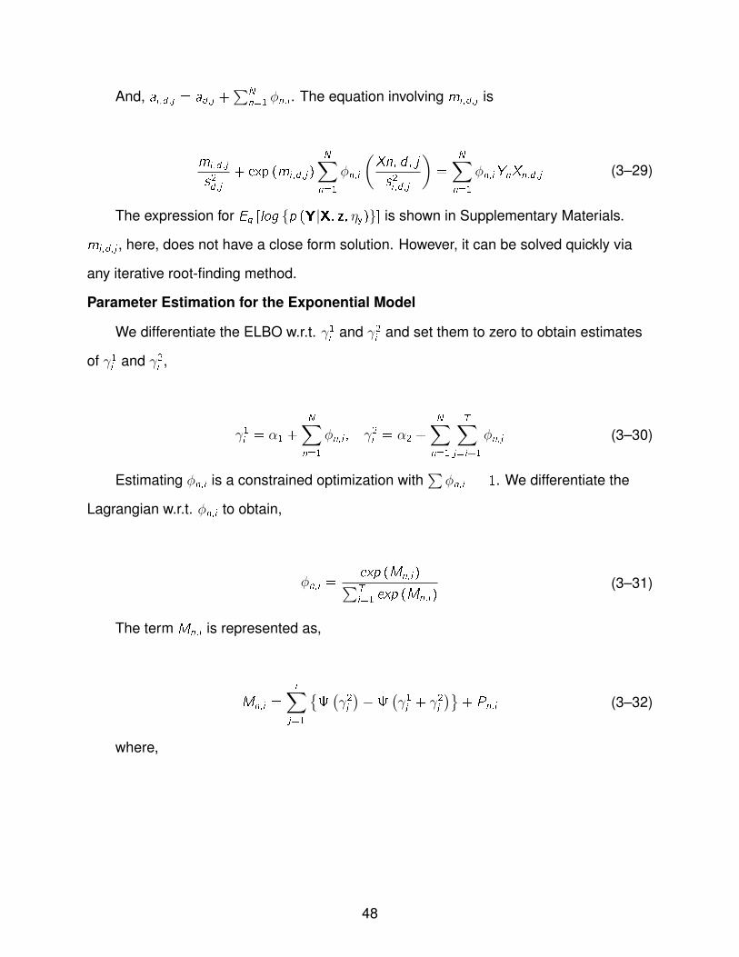
n=1 ϕn,i . The equation involving mi ,d ,j is
mi ,d ,j
s2d ,j+ exp (mi ,d ,j)
N∑n=1
ϕn,i
(Xn, d , j
s2i ,d ,j
)=
N∑n=1
ϕn,iYnXn,d ,j (3–29)
The expression for Eq [log {p (Y|X, z, ηy)}] is shown in Supplementary Materials.
mi ,d ,j , here, does not have a close form solution. However, it can be solved quickly via
any iterative root-finding method.
Parameter Estimation for the Exponential Model
We differentiate the ELBO w.r.t. γ1i and γ2i and set them to zero to obtain estimates
of γ1i and γ2i ,
γ1i = α1 +N∑n=1
ϕn,i , γ2i = α2 +
N∑n=1
T∑j=i+1
ϕn,j (3–30)
Estimating ϕn,i is a constrained optimization with∑ϕn,i = 1. We differentiate the
Lagrangian w.r.t. ϕn,i to obtain,
ϕn,i =exp (Mn,i)∑T
i=1 exp (Mn,i)(3–31)
The term Mn,i is represented as,
Mn,i =
i∑j=1
{(γ2j)−
(γ1j + γ2j
)}+ Pn,i (3–32)
where,
48

Pn,i =
N∑n=1
T∑i=1
D∑d=1
{(ax ,i ,d)− ln (bx ,i ,d)− Xn,d
ax ,i ,d
bx ,i ,d
}+
N∑n=1
T∑i=1
{−cy ,i ,0
dy ,i ,0−
D∑d=1
Xn,d
cy ,i ,d
dy ,i ,d− Yn
� (cy ,i ,0)
(dy ,i ,0 + 1) cy ,i ,0
+Yn
D∑d=1
� (cy ,i ,d)
(dy ,i ,d + Xn,d) cy ,i ,d}
(3–33)
The variational parameters for the covariates and responses are found by maximiz-
ing the ELBO w.r.t. them.
ax ,i ,d = ax ,d +
N∑n=1
ϕn,i , bx ,i ,d = bx ,d +
N∑n=1
ϕn,iXn,d (3–34)
cy ,i ,d = cy ,d +
N∑n=1
(ϕn,i + Yn) , dy ,i ,d = dy ,d +
N∑n=1
ϕn,i (Xn,d + Yn) (3–35)
Parameter Estimation for the Inverse Gaussian Model
For the Inverse Gaussian Model, the estimation of γ1i , γ2i ,ϕn,i are identical to the
Exponential model with the only difference being that Pn,i is given as,
Pn,i =1
2
D∑d=1
{log(
1
2π
)+(cx ,i ,d)− log (dx ,i ,d)
−b−1x ,i ,d −
cx ,i ,d
dx ,i ,d(Xn,d − ax ,i ,d)
2}+ 1
2{log
(1
2π
)+(cy ,i)− log (dy ,i)− b−1
y ,i
(1 +
D∑d=1
X 2n,d
)
−cy ,i
dy ,i
(Yn − ay ,i ,0 −
D∑d=1
ay ,i ,dXn,d
)2
}
(3–36)
49

The variational parameters for the covariates and responses are found by maximiz-
ing the ELBO w.r.t. them.
bx ,i ,d = bx ,d +
N∑n=1
ϕn,i , cx ,i ,d = cx ,d +
N∑n=1
ϕn,i (3–37)
dx ,i ,d =1
2{bx ,d (ax ,i ,d − ax ,d)
2 + 2dx ,d
+
N∑n=1
ϕn,i (Xn,d − ax ,i ,d)2
a2x ,i ,dXn,d
}(3–38)
ax ,i ,d =
∑N
n=1 ϕn,iXn,d + bx ,dmx ,d∑N
n=1 ϕn,i + bx ,d(3–39)
by ,i =(D + 1)by +
∑N
n=1 ϕn,i
(1 +
∑D
d=1 X2n,d
)D + 1
(3–40)
cy ,i =
D∑d=0
cy +1
2
N∑n=1
ϕn,i (3–41)
dy ,i =1
2{
D∑d=0
by (ay ,i ,d − ay ,d)2 + 2dy
+
N∑n=1
ϕn,i
(Yn − ay ,i ,0 −
∑D
d=1 ay ,i ,dXn,d
)2(ay ,i ,0 −
∑D
d=1 ay ,i ,d
)2Xn,d
}
(3–42)
ay ,i ,0 =
ay ,dby +∑N
n=1 ϕn,i
(Yn −
∑D
d=1 ay ,i ,dXn,d
)by +
∑N
n=1 ϕn,i
(3–43)
50

ay ,i ,d =ay ,dby
by +∑N
n=1 ϕn,iX2n,d
+
∑N
n=1 ϕn,i (Yn − ay ,i ,0 + ay ,i ,dXn,d)
by +∑N
n=1 ϕn,iX2n,d
−∑N
n=1 ϕn,i∑D
d=1 ay ,i ,dXn,d
by +∑N
n=1 ϕn,iX2n,d
(3–44)
Parameter Estimation for the Multinomial Probit Model
Once again, in the Multinomial Model, estimation of γ1i , γ2i , ax ,i ,d , bx ,i ,d , cx ,i ,d , dx ,i ,d , are
similar to the Exponential model. The variational parameters are given by,
ay ,i ,k = ay ,k +
N∑n=1
ϕn,i , by ,i ,k = by ,k (3–45)
And, my ,i ,0,k = my ,d ,k + s2y ,d ,k∑N
n=1 ϕn,iYn,k
my ,i ,d ,k = my ,d ,k + s2y ,d ,k
N∑n=1
ϕn,iYn,kXn,d (3–46)
Predictive Distribution
Finally, we derive the predictive distribution for a new response given a new covari-
ate and the set of previous covariate-response pairs.
p (YN+1|XN+1,X,Y) =∑z
∫ ∫p (YN+1|XN+1, ηy, z) p (v, ηy|Y,X) p (z|v) dvdηy
(3–47)
Since the inner integrals are analytically intractable, we approximate the predictive
distribution by replacing the true posterior with its variational surrogate. The density,
51

q(v), is integrated out to give the weight factor wi for each mixture. The remaining part is
integrated out to produce a t-distribution for the Normal model.
p (YN+1|XN+1,X,Y)
=
T∑i=1
wiSt
(Y |
(my ,i ,0 +
D∑d=1
my ,i ,dXN+1,d ,Li ,Bi
)) (3–48)
Here, wi is given by,
wi =γ1i γ
2i
(γ2i + 1
).............
(γ2i + T − 1− i
)(γ1i + γ2i ) (γ
1i + γ2i + 1) ........ (γ1i + γ2i + T − i)
(3–49)
Here, Li =(2ay ,i−D)βy ,i2(1+βy ,i)by ,i
, which is the precision parameter of the Student’s t-
distribution and Bi = 2ay ,i −D is the degrees of freedom.
For the other models, the integration of the densities q (ηy ,i) and p (YN+1) is not
analytically tractable. Therefore, we use Monte Carlo integration to obtain,
E [YN+1|XN+1,X,Y] = E[E[YN+1|XN+1, ηy,i(1:T)
]|X,Y
]=
1
M
M∑m=1
E[YN+1|XN+1, η
my,i(1:T)
] (3–50)
In all experiments presented in this dissertation, we collected 100 i.i.d. samples
from the density of ηy ,i to evaluate the expected value of YN+1 from the density of
p (YN+1).
Experimental Results
A broad set of experiments were conducted to evaluate the variational inference
and a standard Gibbs sampling. Samples from the predictive posterior were used to
evaluate the accuracy of the model against its competitor algorithms, such as, linear
regression with no feature selection (OLS), Bayesian Linear regression, variational
linear regression Bishop (2006), Gaussian Process regression Rasmussen and Williams
52

Table 3-1. Description of variational inference algorithms for the modelsInitialize hype-parameters of the generative model.RepeatEvaluate γ1i and γ2i .Evaluate ϕn,i of the respective Model.Evaluate variational parameters of the covariate distribution.Evaluate variational parameters of the response distribution.until converged
Figure 3-1. A simple posterior predictive trajectory of variational inference of the normalmodel in a 4 cluster synthetic dataset with a 1-D covariate. The ”blue”trajectory is the smoothed response posterior trained in the 4 cluster datarepresented by the points.
(2005a), ordinary DP regression and the Gibbs sampling inferenceHannah et al. (2011).
Variational inference’s speed of convergence was also recorded and compared against
that of Gibbs sampling, for successively growing dimensionality of the covariates.
The accuracy of the Multinomial and Probit models model (variational inference) was
evaluated against multiclass support vector machine Cortes and Vapnik (1995), naive
Bayes classifier Lowd and Domingos (2005) and multinomial logistic regression Bishop
(2006).
Next, to highlight the models as a practical tool, it was employed as a new GLM-
based technique to model the volatility dynamics of the stock market. Specifically, it
was used to determine how individual stocks tract predetermined baskets of stocks over
time.
53

Datasets
One artificial group of datasets and three real world datasets were used. In the
artificial set, we generated several 25 to 100 dimensional regression datasets with 10
clusters each in the covariate-response space (Y ,X ). The covariates were generated
from independent Gaussians with means varying from 1 to 27 in steps of 3 for the
10 clusters. The shape parameter was drawn independently from the range [.1, 1]
for the 10 clusters. For a fixed cluster, the shapes were set to be the same for each
dimension. The second dataset was a compilation of daily stock price data (retrieved
from Google finance) for the ”Dow 30” companies from Nov 29, 2000 to Dec 29, 2013. It
had 3268 instances and was viewed as 30 different 29-1 covariate-response datasets.
The goal was to model the stock price of an individual Dow-30 company as a function
of the remaining 29 companies, over time. Accuracy results were averaged over all 30
regressions. The third dataset was the Parkinson’s telemonitoring dataset A. Tsanas
and Ramig (2009) from the UCI Machine Learning Repository that has 5875 instances
over 16 covariates. The final dataset was the Breast Cancer Wisconsin (Original)
dataset Wolberg and Mangasarian (1990) from the UCI Repository that has 699
instances over 10 covariates. This dataset was used to evaluate Multinomial and Probit
Models against competitors like multiclass SVM Cortes and Vapnik (1995), Multinomial
Logistic regression Bishop (2006) and naive Bayes classifier Lowd and Domingos
(2005).
Timing Performance for the Normal Model
For a fair comparison of computing time, we ran both variational inference and
Gibbs sampling to convergence for 50 percent of the dataset set to train. For Gibbs
sampling, we assessed convergence to the stationary distribution using the Gelman-
Rubin diagnostic Gelman and Wolberg (1992). For variational inference, we measured
convergence using the relative change of the ELBO, stopping the algorithm when it
was less than 1e-8. The variation of timing for both variational inference and Gibbs
54

Figure 3-2. Time in seconds per dimension for both variational inference and Gibbssampling for the synthetic dataset.
Table 3-2. Run time per dimension for convergence of Gibbs sampling and variationalinference in seconds.
Stock market data Telemonitoring dataVariational inference 436.34 229.97Gibbs sampling 521.65 311.12Synthetic datasetDimension 25 40 50 60 75 100Variational inference 320 290 280 275 270 240Gibbs sampling 495 680 875 995 1240 1475
sampling per dimension for all the datasets are tabulated in Table 3-2. Gibbs sampling
remains close to variational inference in the telemonitoring dataset which has only 16
covariates. However, as shown in the synthetic data, when the dimensionality grows
from 25 to 100, Gibbs sampling starts to lag behind variational inference, exposing its
vulnerability to growing dimensions. In contrast, variational inference remains robust
against rising dimensionality of the covariates where its time consumption per dimension
for convergence decreases slightly as the dimensionality increases.
Accuracy
We report the mean absolute error (MAE) and Mean Square Error (MSE) for all
the algorithms in Table 3-4 Note that variational inference yields the least error values
among its competitors. To compare variational inference with Gibbs sampling, we set the
55

Table 3-3. Log-likelihood of the normal model of the predictive distribution for thesynthetic dataset(50,75,100 dimensions) and stock market and telemonitoringdataset(30, 60 and 90 % of data set as training).
Synthetic datasetDimension Variational inference Gibbs sampling50 -2345.05 -2789.8375 -3729.38 -4589.49100 -4467.75 -6052.62Stock market datasetTraining percentage Variational inference Gibbs sampling30 -912.58 -1254.7860 -834.29 -1087.9290 -712.82 -878.99Telemonitoring datasetTraining percentage Variational inference Gibbs sampling30 -673.55 -794.2960 -545.17 -643.4890 -487.77 -529.82
truncation factor (T ) to 20 and the samples of Gibbs sampling were taken after burn-in
to be every 5th sample.
We show the log-likelihood of the Normal model of the predictive distribution in Ta-
ble 3-3 with dimension varied from 50 to 100 for the synthetic dataset (50 percent of the
data set as training) and also for the compiled stock market and telemonitoring dataset
(30,60 and 90 percent of the data set as training). It is notable that Gibbs sampling
deteriorates very quickly as the dimensionality of the covariates grows larger (from 16
dimensional in telemonitoring to 50-100 dimensional in the synthetic dataset). In terms
of the MSE and MAE too, Gibbs sampling shows the same trend. Errors are low in the
telemonitoring datasets, but with increasing dimensions, as in the synthetic and stock
market data, it loses scalability since its sample distribution strays substantially from the
true posterior, thus leading to large errors.
Tool to Understand Stock Market Dynamics
The models are presented as new tools to analyze the dynamics of stocks from
the ”Dow 30” companies. ”Dow 30” stocks belong to disparate market sectors such
56

Table 3-4. MSE and MAE of the algorithms for the synthetic dataset(50,75,100dimensions), stock market dataset, telemonitoring data set and breast cancerdataset with 30, 60 and 90 % of data set as training.
Synthetic data MAE MSETraining percent 30 60 90 30 60 90Variational inference (normal model) 1.04 .82 .67 1.72 1.59 1.31Gibbs sampling (normal model) 1.45 1.23 1.02 1.61 1.45 1.32Variational inference (inverse Gaussian model) 1.21 .89 .79 1.78 1.55 1.39Variational inference (exponential model) 1.32 1.26 1.16 1.85 1.78 1.44ODP 1.47 1.37 1.29 1.95 1.82 1.52GPR 1.56 1.42 1.63 2.34 2.17 1.79VLR 1.71 1.53 1.29 2.49 2.28 2.82BLR 1.92 1.59 1.41 2.71 2.44 1.92LR 1.55 1.47 1.36 2.78 2.57 2.12Stock market data MAE MSETraining percent 30 60 90 30 60 90Variational inference (normal model) .87 .71 .62 1.54 1.41 1.24Gibbs sampling (normal model) 1.32 .99 .90 1.78 1.67 1.56Variational inference (Inverse Gaussian model) .74 .63 .56 1.39 1.28 1.13Variational inference (exponential model) 1.01 .92 .79 1.62 1.51 1.40ODP .99 .88 .73 1.74 1.57 1.38GPR .83 .76 .68 1.53 1.44 1.29VLR 1.07 .99 .90 1.82 1.71 1.50BLR 1.16 1.05 .92 1.89 1.76 1.56LR 1.25 1.13 1.01 1.94 1.83 1.64Telemonitoring data MAE MSETraining percent 30 60 90 30 60 90LR 1.86 1.55 1.36 2.09 1.66 1.36BLR 1.91 1.60 1.32 2.13 1.63 1.30VLR 1.88 1.52 1.28 2.07 1.70 1.33ODP 1.85 1.59 1.33 2.10 1.64 1.29GPR 1.80 1.56 1.27 2.04 1.57 1.26Variational inference (Inverse Gaussian model) 1.79 1.54 1.25 2.01 1.59 1.25Variational inference (exponential model) 1.77 1.48 1.23 1.99 1.53 1.20Gibbs sampling (normal model) 1.81 1.59 1.30 1.80 1.67 1.35Variational inference (normal model) 1.58 1.39 1.17 1.82 1.65 1.51Breast cancer data Class percentage accuracyTraining percent 30 60 90Variational inference (Probit model) 86.4 92.1 98.3Variational inference (multinomial model) 90.4 95.1 98.8Naive Bayes 69.7 76.9 82.8SVM 74.4 78.7 86.9Logistic 75.3 81.2 89.5
57

Table 3-5. List of five different stocks with top 3 most significant stocks that influenceeach stock. Here, Intel, Verizon, Cisco, IBM, AT-T are tech. stocks, MMM,CAT, DD, Boeing, GE are machinery/chemical stocks, XOM, Chevron areenergy stocks, AXP, GS, PG, TRX, JPM, VISA are finance/retail stocks andMCD, J-J, Coca-Cola are food stocks.
Time-period Cisco Goldman sachs Chevron McDonald Boeing
2000-07Verizon JPM XOM J and J DDIBM VISA Boeing Coca-Cola GEGE AXP MMM NKE GS
2007-09AXP XOM AT-T MMM MCDINTEL NKE PG IBM VISADIS DD Coca-Cola TRX MMM
2009-13INTEL AXP XOM Coca-cola CATMSFT PG CAT Merck DDDD JPM GE J and J JPM
as, technology (Microsoft, Intel etc.), finance (Goldman Sachs, American Express
etc.), food/pharmaceuticals (Coca-cola, McDonald,Johnson and Johnson), Energy and
Machinery (Chevron, GE, Boeing, Exxon Mobil). We divided the dataset into 3 time
segments on the two sides of the financial crisis of 2008. The first comprised of the
stock values from Nov-00 to Nov-07 and the third of the stock values from Dec08-Dec13.
The middle, set as the remainder, was representative of the financial crisis.
Using the models, we modeled each company’s stock value as a function of the
values of the others in DOW 30. We recorded the stocks having the most impact on the
determination of the value of each stock. The impacts are necessarily the magnitude
of the weighted coefficients of the covariates (the stock values) in the models. Two
significant trends were noteworthy.
Firstly, when the market was stable (the first and third segments), stocks from any
given sector had impact largely on the same sector, with few stocks being influential
overall. Secondly, the sectors having the most impact on a specific stock were the same
on both sides of the crisis. For example, Microsoft (tech. sector), is largely modeled by
Intel, IBM (tech), GE (machinery) and JPM (finance) previous to the crisis and modeled
by Cisco, Intel (tech), Boeing (machinery) and GS (finance) (in descending order of
58

weights) post crisis. However, during the crisis, the stocks showed no such trends. For
example, Microsoft is impacted by GS, MMM, TRX and Cisco showing no sector wise
trend. We report 5 additional such results in Table 3-5. All the results are for the Inverse
Gaussian Model. But they are quite similar for the other models also.
59

CHAPTER 4AUTOMATIC DETECTION OF LATENT COMMON CLUSTERS OF GROUPS IN
MULTIGROUP REGRESSION
Models Related to iMG-GLM
After its introduction, Generalized Linear Model was extended to Hierarchical Gen-
eralized Linear Model (HGLM) Lee and Nelder (1996). Then structured dispersion was
included in Lee and Nelder (2001a) and models for spatio-temporal co-relation were
proposed in Lee and Nelder (2001b). Generalized Linear Mixed Models (GLMMs) were
proposed in Breslow and Clayton (1993). The random effects in HGLM were specified
by both mean and dispersion in Lee and Nelder (2006). Mixture of Linear Regression
was proposed in Viele and Tong (2002). Hierarchical mixture of regression was pre-
sented in Jordan and Jacobs (1993). Varying coefficient models were proposed in
Hastie and Tibshirani (1993). Multi-tasking Model for classification in a Non-parametric
Bayesian scenario was introduced in Ya Xue and Carin (2007). Sharing Hidden Nodes
in Neural Networks was introduced in Baxter (1995, 2000). General Multi-Task learning
was described first in Caruana (1997). Common prior in hierarchical Bayesian model
was used in Yu et al. (2005); Zhang et al. (2005). Common structure sharing in the
predictor space was presented in Ando and Zhang (2005).
All of these models suffer the shortcomings of not identifying the latent clustering
effect across groups as well as varying uncertainty with respect to covariates across
groups, which the iMG-GLMs presented here inherently models.
iMG-GLM Model Formulation
We consider M groups indexed by j = 1, ....,M and the complete data as D =
{xj ,i , yj ,i} s.t. i = 1, ...Nj . {xj ,i , yj ,i} are covariate-response pairs and are drawn i.i.d. from
an underlying density which differs along with the nature of {xj ,i , yj ,i} among various
models.
60

Figure 4-1. Graphical representation of iMG-GLM-1 model.
Normal iMG-GLM-1 Model
In the Normal iMG-GLM-1 model, the generative model of the covariate-response
pair is given by the following set of equations. Here, Xji and Yji represent the i th con-
tinuous covariate-response pairs of the j th group. The distribution of Yj ,i |Xj ,i is normal
parametrized by β0:D and λ. The distribution, {βkd ,λk} (Normal-Gamma) is the prior
distribution on the covariate coefficient β. This distribution is the base distribution (G)
of the Dirichlet Process. The set {m0, β0, a0, b0} constitute the hyper-parameters for the
covariate coefficients (β) distribution. The graphical representation of the normal model
is given in Figure 4.
vk ∼ Beta(α1,α2), πk = vk�k−1n=1 (1− vn)
N(βkd |m0, (β0,λk)
−1)Gamma (λk |a0, b0)
Zj |vk ∼ Categorical (π1, ......π∞)
Yji |Xji ∼ N(Yji |
∑Dd=0 βZjdXjid ,λ
−1Zj
)(4–1)
61

Logistic Multinomial iMG-GLM-1 Model
In the Logistic Multinomial iMG-GLM-1 model, a Multinomial Logistic Framework
is used for a Categorical response, Yji , for a continuous covariate, Xji , in the case of
i th data point of the j th group. t is the index of the category. The distribution of Yj ,i |Xj ,i
is Categorical parametrized by β0:D,0:T . The distribution, {βktd} (Normal) is the prior
distribution on the covariate coefficient β which is the base distribution (G) of the
Dirichlet Process. The set {m0, s0} constitute the hyper-parameters for the covariate
coefficients (β) distribution.
vk ∼ Beta(α1,α2), πk = vk�k−1n=1 (1− vn)
βktd ∼ N(βktd |m0, s
20
), Zj |vk ∼ Categorical (π1, ......π∞)
Yji = t|Xji ,Zj ∼exp
(∑Dd=0 βZj tdXjid
)∑T
t=1 exp(∑D
d=0 βZj tdXjid
)(4–2)
Poisson iMG-GLM-1 Model
In the Poisson iMG-GLM model, a Poisson distribution is used for the count re-
sponse. Here, Xji and Yji represent the i th continuous/ordinal covariate and categorical
response pair of the j th group. The distribution of Yj ,i |Xj ,i is Poisson parametrized by
β0:D,0:T . The distribution, {βkd} (Normal) is the prior distribution on the covariate co-
efficient β which is the base distribution (G) of the Dirichlet Process. The set {m0, s0}
constitute the hyper-parameters for the covariate coefficients (β) distribution.
vk ∼ Beta(α1,α2), πk = vk�k−1n=1 (1− vn) ,
{βk,d} ∼ N(βkd |m0, s
20
)Yji |Xji ,Zj ∼ Poisson
(yji | exp
(∑Dd=0 βZjdXjid
)) (4–3)
Variational Inference
The inter-coupling between Yji , Xji and zj in all three models described above
makes computing the posterior of the latent parameters analytically intractable. We
62
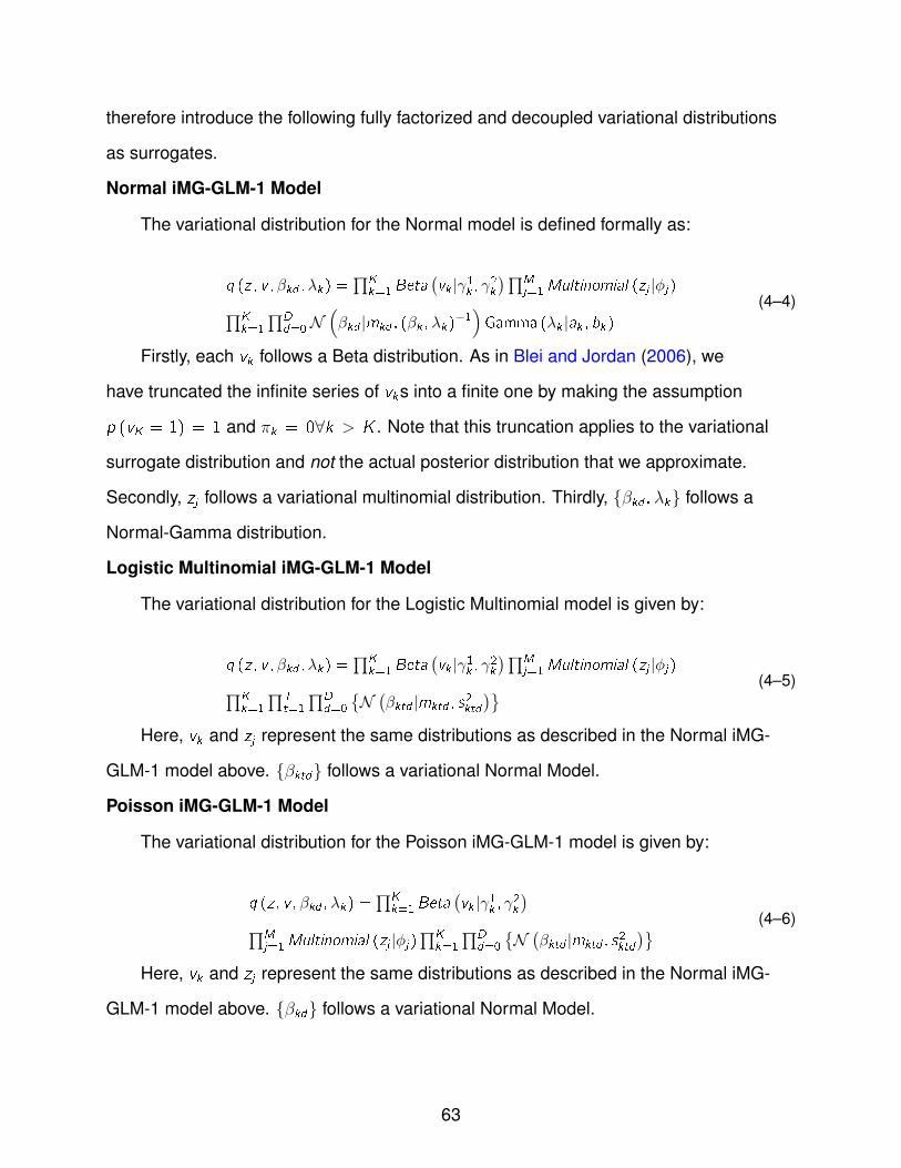
therefore introduce the following fully factorized and decoupled variational distributions
as surrogates.
Normal iMG-GLM-1 Model
The variational distribution for the Normal model is defined formally as:
q (z , v ,βkd ,λk) =∏K
k=1 Beta(vk |γ1k , γ2k
)∏Mj=1Multinomial (zj |ϕj)∏K
k=1
∏Dd=0N
(βkd |mkd , (βk ,λk)
−1)Gamma (λk |ak , bk)
(4–4)
Firstly, each vk follows a Beta distribution. As in Blei and Jordan (2006), we
have truncated the infinite series of vks into a finite one by making the assumption
p (vK = 1) = 1 and πk = 0∀k > K . Note that this truncation applies to the variational
surrogate distribution and not the actual posterior distribution that we approximate.
Secondly, zj follows a variational multinomial distribution. Thirdly, {βkd ,λk} follows a
Normal-Gamma distribution.
Logistic Multinomial iMG-GLM-1 Model
The variational distribution for the Logistic Multinomial model is given by:
q (z , v ,βkd ,λk) =∏K
k=1 Beta(vk |γ1k , γ2k
)∏Mj=1Multinomial (zj |ϕj)∏K
k=1
∏Tt=1
∏Dd=0
{N(βktd |mktd , s
2ktd
)} (4–5)
Here, vk and zj represent the same distributions as described in the Normal iMG-
GLM-1 model above. {βktd} follows a variational Normal Model.
Poisson iMG-GLM-1 Model
The variational distribution for the Poisson iMG-GLM-1 model is given by:
q (z , v ,βkd ,λk) =∏K
k=1 Beta(vk |γ1k , γ2k
)∏M
j=1Multinomial (zj |ϕj)∏K
k=1
∏Dd=0
{N(βktd |mktd , s
2ktd
)} (4–6)
Here, vk and zj represent the same distributions as described in the Normal iMG-
GLM-1 model above. {βkd} follows a variational Normal Model.
63
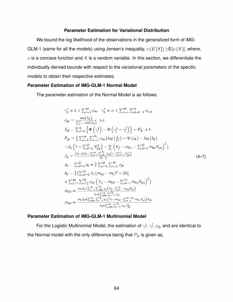
Parameter Estimation for Variational Distribution
We bound the log likelihood of the observations in the generalized form of iMG-
GLM-1 (same for all the models) using Jensen’s inequality, ϕ (E [X ])≥E[ϕ (X )], where,
ϕ is a concave function and X is a random variable. In this section, we differentiate the
individually derived bounds with respect to the variational parameters of the specific
models to obtain their respective estimates.
Parameter Estimation of iMG-GLM-1 Normal Model
The parameter estimation of the Normal Model is as follows:
γ1k = 1 +∑M
i=1 ϕik , γ2k = α+∑M
i=1
∑Kp=k+1 ϕn,p
ϕjk =exp(Sjk)∑Kk=1 exp(Sjk)
s.t.
Sjk =∑k
j=1
{(γ1j
)−
(γ1j + γ2j
)}+ Pjk s.t.
Pjk = 12
∑Mj=1
∑Nj
i=1 ϕjk{log(12π
)+(ak)− log (bk)
−βk(1 +
∑Dd=1 X
2jid
)− ak
bk
(Yji −mk0 −
∑Dd=1mkdXjid
)2}
βk =(D+1)β0+
∑Mj=1
∑Nj
i=1ϕjk(1+
∑Dd=1 X
2jid)
D+1
ak =∑D
d=0 a0 +12
∑Mj=1
∑Nj
i=1 ϕjk
bk = 12{∑D
d=0 β0 (mkd −m0)2 + 2b0
+∑M
j=1
∑Nj
i=1 ϕjk
(Yji −mk0 −
∑Dd=1mkdXjid
)2}
mk0 =m0β0+
∑Mj=1
∑Nj
i=1ϕji(Yji−
∑Dd=1mkdXjid)
β0+∑M
j=1
∑Nj
i=1ϕjk
mkd =m0β0+
∑Mj=1
∑Nj
i=1ϕji
(Yji−mk0−
∑D−(d)d=1
mkdXjid
)Xjid
β0+∑M
j=1
∑Nj
i=1ϕjkX
2jid
(4–7)
Parameter Estimation of iMG-GLM-1 Multinomial Model
For the Logistic Multinomial Model, the estimation of γ1i , γ2i ,ϕjk and are identical to
the Normal model with the only difference being that Pjk is given as,
64

Pjk = 12
∑Mj=1
∑Nj
i=1 ϕjk{log(12π
)+∑T
t=1 Yjit
(mk0t +
∑Dd=1 Xjidmkdt
)mkdt = m0s
20 + s2kdt
∑Mj=1 ϕjk
∑Nj
j=1 YjitXjid , s2kdt = s20+∑Mj=1 ϕjk
∑Nj
j=1
(∑Dd=0 X
2jid exp
(∑Dd=0 Xjidmkdt
))(4–8)
Parameter Estimation of Poisson iMG-GLM-1 Model
Again, in the Poisson Model, estimation of γ1i , γ2i ,ϕjk , are similar to the Normal
model with the only difference being that the term Pjk is given as,
Pjk = 12
∑Mj=1
∑Nj
i=1 ϕjk{−∑D
d=0 exp(skd
2 +mkdXjid
skd
)+
Yji
(∑Dd=0 Xjidmkd
)− log (Yji)
mkd
s2kd
+ exp (mkd) +∑M
j=1 ϕjk∑Nj
i=1Xjid
s2kd
=∑M
j=1
∑i=1 NjϕjkYjiXjid
(4–9)
For, mkd and skd , does not have a close form solution. However, it can be solved
quickly via any iterative root-finding method.
Predictive Distribution
Finally, we define the predictive distribution for a new response given a new covari-
ate and the set of previous covariate-response pairs for the trained groups.
p (Yj ,new |Xj ,new ,Zj ,βk=1:K ,d=0:D) =∑Kk=1
∫Zjkp
(Yj ,new |Xj ,new ,β
Dk,d=0
)q (z , v ,βkd ,λk)
(4–10)
Integrating out the q (z , v , βkd ,λk), we get the following equation for the Normal
model.
p (Yj ,new |Xj ,new ) =∑Kk=1 ϕjkSt
(Yj ,new |
(∑Dd=0mkdXj ,new ,,d ,Lk ,Bk
)) (4–11)
Here, Lk = (2ak−D)βk2(1+βk)bk
, which is the precision parameter of the Student’s t-distribution
and Bi = 2ay ,i − D is the degrees of freedom. For the Poisson and Multinomial Models,
65

Table 4-1. Description of variational inference algorithm for iMG-GLM-1 normal model1. Initialize generative model latent parameters q (z , v , βkd ,λk)randomly in its state space.Repeat2. Estimate γ1k and γ2k . for k = 1 to K .3. Estimate ϕjk . for j = 1 to M and for k = 1 to K .4. Estimate the model density parameters, {mkd , βk , ak , bk}for k = 1 to K and d = 0 to D.until converged5. Evaluate E [Yj ,new ] for a new covariate, Xj ,new
the integration of the densities is not analytically tractable. Therefore, we use Monte
Carlo integration to obtain,
E [Yj ,new |Xj,new,X,Y] = E [E [Yj ,new |Xj,new,q (βkd)] |X,Y]
= 1S
∑Ss=1 E [Yj ,new |Xj,new,q (βkd)]
(4–12)
In all experiments presented in this dissertation, we collected 100 i.i.d. samples
(S=100) from the density of β to evaluate the expected value of Yj ,new . The complete
variational inference algorithm for iMG-GLM-1 Normal Model is given Table 4-1.
iMG-GLM-2 Model
We can now learn a new group M + 1, after all of the first M groups have been
trained. For this process, we memorize the learned latent parameters from the previ-
ously learned data.
Information Transfer from Prior Groups
First, we write down the latent parameter conditional distribution given all the
parameters in the previous groups. We define the set of latent parameters (Z , v , β,λ) as
η. From the description of Dirichlet Process we write down the probability for the latent
parameters for the (M + 1)th group given previous ones,
p (ηM+1|η1:M ,α,G0) =α
M+αG0 +1
M+α
∑Kk=1 nkδη∗k
(4–13)
Where, nk =∑M
j=1 Zjk , represents count where ηj = η∗k . If we substitute η∗k = E [η∗k ],
which we define by = {ϕjk , γk ,mdk ,λk , sdk}, we get,
66

p(ηM+1|η∗k ,α,G0
)= α
M+αG0 +1
M+α
∑Kk=1 nkδη∗k
(4–14)
Where, nk =∑M
j=1 indexjk and indexjk = δargmax(ϕjk). This distribution represents the
prior belief about the new group latent parameters in the Bayesian setting. Now our goal
is to compute the posterior distribution of the new group latent parameters after we view
the likelihood with the data in (M + 1)th group.
p (ηM+1|,α,DM+1) =p(DM+1|ηM+1)p(ηM+1|,G0)
p(DM+1|,G0)(4–15)
Here, p (DM+1|ηM+1) = �NM+1
i=1 p (YM+1,i |ηM+1,XM+1,i).
Posterior Sampling
The posterior above does not have a closed form solution apart from the Normal
Model. So, we apply a Metropolis Hastings Algorithm Robert and Casella (2005);
Neal (2000b) for the Logistic Multinomial and Poisson Model. For the Normal model,
p (ηM+1|,α,DM+1) turns out to be a mixture of Normal-Gamma density with following
parameters,
m∗k =
{XTM+1XM+1 + (βk) I
}−1 {XTM+1YM+1 + βk Imk
}β∗k =
(XTM+1XM+1 + βk I
), a∗k = ak + NM+1/2
b∗k = bk +12
{Y TM+1YM+1 +mT
k βkmk −m∗Tk β∗km
∗k
} (4–16)
For the Poisson and Logistic Multinomial Model, the Metropolis Hastings Algorithm
has the following steps. First, we draw a sample _η from above. Then we draw a candi-
date sample η, Next, we compute the acceptance probability,[min
[1, p(DM+1|η)
p(DM+1| _η)
]]. We
set the new _η to η with this acceptance probability. Otherwise, it remains the old value.
We repeat the above 4 steps until enough samples has been collected. This yields the
approximation of the posterior.
67

Prediction for New Group Test Samples
We seek to predict the future YM+1,new |XM+1,new , , by the following equation with
the previous collection of posterior samples ηt=1:T . T is the number of samples.
p (YM+1,new |XM+1,new , )
= 1T
∑Tt=1 p (YM+1,new |XM+1,new , ηt)
(4–17)
Experimental Results
We present empirical studies on two real world applications: (a) a Stock Market
Accuracy and Trend Detection problem and (b) a Clinical Trial problem on the efficacy of
a new drug.
Trends in Stock Market
We propose iMG-GLM-1 and iMG-GLM-2 as a trend spotter in Financial Markets
where we have chosen daily close out stock prices over 51 stocks from NYSE and
Nasdaq in various sectors, such as, Financials (BAC, WFC, JPM, GS, MS, Citi, BRK-B,
AXP), Technology (AAPl, MSFT, FB, GOOG, CSCO, IBM, VZ), Consumer Discretionary
(AMZN, DIS, HD, MCD, SBUX, NKE, LOW), Energy (XOM, CVX, SLB, KMI, EOG),
Health Care (JNJ, PFE, GILD, MRK, UNH, AMGN, AGN), Industrials (GE, MMM, BA,
UNP, HON, UTX, UPS), Materials (DOW, DD, MON, LYB) and Consumer Staples (PG,
KO, PEP, PM, CVS, WMT). The task is to predict future stock prices given past stock
value for all these stocks and spot general trends in the cluster of the stocks which might
be helpful in finding a far more powerful model for prediction. The general setting is
a auto-regressive process via the Normal iMG-GLM-1 model with lags representing
the predictor variables and response being the current stock price. The lag-length
was determined to be 3 by trial and error with 50-50 training-testing split. Data was
collected from September 13th, 2010 to September 13th, 2015 with 1250 data points,
from Google Finance.
68

Some very interesting trends were noteworthy. After the clustering was accom-
plished for the Normal model, the stocks became grouped almost entirely by the sectors
they came from. Specifically, we witnessed a total of 9 clusters of stocks, close in
makeup to the 8 sectors chosen originally consolidating all the stocks sectors such as,
financial, healthcare etc. For example, Apple, Microsoft Verizon, Google, Cisco and
AMZN were clubbed together in one cluster. This signifies that all of these stocks share
the same auto-regressive density with the same variance. In comparison, single and
separate modeling of the stocks resulted in a much inferior model. Joint modeling was
particularly useful because we had only 625 data points per stocks for training purposes
over the past 5 years. As a result, transfer of stock data points from one stock to another
helped mitigate the problem of over-fitting the individual stocks while ensuring a much
improved model for density estimation for a cluster of stocks. We report the clustering
of the stocks in Table 4-2. We also show the accuracy of the prediction for the iMG-
GLM-1 model in terms of the Mean Absolute error (MAE) in Table 4-3. Note that MAE
for the Normal model significantly outperformed the GLMM normal model, stock specific
Random Forest, Linear Regression and Gaussian Process Regression.
We now highlight the utilization of information transfer in the iMG-GLM-1 model.
We trained the first 51 stocks where we varied the number of training samples in each
group/stock from 200 to 1200 in steps of 250. For each group we chose the training
samples randomly from the datasets and the remaining were used for testing. The
hyper-parameters were set as, {m0, β0, a0, b0} = 0, 1, 2, 2. We also ran our inference with
different settings of the hyper-parameters but found the results not to be particularly
sensitive to the hyper-parameters settings. We plot the average MAE of 50 random
runs in Figure 4. The iMG-GLM-1 Normal Model generally outperformed the other
competitors. Few interesting results were found in this experiment. When very few
training samples were used for training, virtually all the algorithms performed poorly.
In particular, iMG-GLM-1 clubbed all stocks into one cluster as sufficient data was not
69

present to identify the statistical similarities between stocks. As the number of training
samples increased iMG-GLM-1 started to pick out cluster of groups/stocks as it was
able find latent common densities among different groups. As, the training samples got
closer to the number of data points (1200), all other models started to perform close
to the iMG-GLM-1 model, because they managed to learn each stock well in isolation,
indicating that further data from other groups became less useful.
We now proceed to iMG-GLM-2, where we trained 10 new stocks from different
sectors (CMCSA, PCLN, WBA, COST, KMI, AIG, GS, HON, LMT, T). Two features
which influenced the learning were considered. First, we varied the number of training
samples from 400 to 750 to 1100 for each previous groups that were used to further
train βM+1. Then, we changed the number of training samples for the new groups from
200 to 1200 in steps of 250. We plot the MAE results for 50 random runs in Figure 4.
The prior belief is that the new groups are similar in response density to the previous
groups. iMG-GLM-2 efficiently transfers this information from a previous groups to new
groups. The iMG-GLM-1 model learns an informative prior for new groups when the
number of training samples for each previous group is very small (as seen in the first
part in Figure 4). The accuracy increases very slightly as the number of training samples
increases in each group. But, with the number of training samples for the new groups
increasing, iMG-GLM-2 does not improve at all. This is due to the flexible information
transfer from the previous groups. The model does not require more training samples for
its own group to model its density, because it has already obtained sufficient information
as prior from the previous groups.
Clinical Trial Problem Modeled by Poisson iMG-GLM Model
Finally, we explored a Clinical Trial problem IBM (2011) for testing whether a
new anticonvulsant drug reduces a patient’s rate of epileptic seizures. Patients were
assigned the new drug or the placebo and the number of seizures were recorded
over a six week period. A measurement was made before the trial as a baseline. The
70

Table 4-2. Clusters of Stocks from Various Sectors. We note 9 clusters of stocksconsolidating all the pre-chosen sectors such as, financials, materials etc.Group numbers are indexed from 1 to 9.
1 2 3 4 5 6 7 8 9AAPLMSFT
VZGOOGCSCOAMZN
BACWFCJPMAXP
PG, CITIGS, MS
DISHD
LOWSBUXMCD
XOMCVXSLBEOGKMI
GILDMRKUNH
AMGNAGN
GEMMM
BAUNPHON
DOWDD
MONLYBJNJPFE
KOPEPPM
CVSWMT
BRK-BIBMFB
NKEUTXUPS
Table 4-3. Mean absolute error for all stocks. iMG-GLM-1 has much higher accuracythan other competitors.
AAPL MSFT VZ GOOG CSCO AMZN BAC WFC JPM AXP PG CITI GS MS DIS HD LOWGPR .023 .004 .087 .078 .093 .189 .452 .265 .176 .190 .378 .018 .037 .098 .278 .038 .011RF .278 .903 .370 .256 .290 .570 .159 .262 .329 .592 .746 .894 .956 .239 .934 .189 .045LR .381 .865 .280 .038 .801 .706 .589 .491 .391 .467 .135 .728 .578 .891 .389 .790 .624GLMM .378 .489 .389 .208 .972 .786 .289 .768 .189 .389 .590 .673 .901 .490 .209 .391 .991iMG-GLM .012 .002 .009 .011 .018 .028 .047 .038 .035 .079 .069 .087 .019 .030 .139 .189 .213
SBUX MCD XOM CVX SLB EOG KMI GILD MRK UNH AMGN AGN GE MMM BA UNP HONGPR .837 .289 .849 .583 .185 .810 .473 .362 .539 .289 .306 .438 .769 .848 .940 .829 .691RF .884 .321 .895 .843 .774 .863 .973 .729 .894 .794 .695 .549 .603 .738 .481 .482 .482LR .380 .391 .940 .995 .175 .398 .539 .786 .591 .320 .793 .839 .991 .839 .698 .389 .298GLMM .649 .720 .364 .920 .529 .369 .837 .630 .729 .481 .289 .970 .740 .649 .375 .439 .539iMG-GLM .003 .018 .128 .291 .005 .060 .052 .017 .014 .078 .009 .067 .191 .034 .098 .145 .238
DOW DD LYB JNJ PFE KO PEP PM CVS WMT BRK-B IBM FB NKE UTX UPS MONGPR .689 .890 .745 .907 .678 .378 .867 .945 .361 .934 .589 .845 .901 .310 .483 .828 .748RF .181 .098 .489 .237 .692 .827 .490 .295 .749 .692 .957 .295 .478 .694 .747 .806 .945LR .67 .386 .984 .982 .749 .294 .256 .567 .345 .767 .893 .956 .294 .389 .694 .921 .702GLMM .727 .389 .288 .592 .402 .734 .923 .900 .571 .312 .839 .956 .638 .490 .390 .372 .512iMG-GLM .038 .078 .063 .019 .024 .007 .089 .192 .138 .111 .289 .390 .289 .218 .200 .149 .087
objective was to model the number of seizures, which being a count datum, is modeled
using a Poisson distribution with a Log link. The covariates are: Treatment Center size
(ordinal), number of weeks of treatment (ordinal), type of treatment–new drug or placebo
(nominal) and gender (nominal). A Poisson distribution with log link was used for the
count of seizures. Here, Xji and Yji represent the i th covariate and count response pair
of the j th group. The distribution, {βkd} (Normal) is the prior distribution on the covariate
coefficient β.
We found that a patient’s number of seizures are clustered (they form the groups) in
multiple collections. This signifies that a majority of the patients across groups show the
same response to the treatment. We obtained 8 clusters from 300 out of 565 patients
for the iMG-GLM-1 model (the remaining 265 were set aside for modeling through the
71

Table 4-4. MSE and MAE of the algorithms for the clinical trial dataset and number ofpatients in clusters for iMG-GLM-1 and iMG-GLM-2 model.
Patient number in clusters for iMG-GLM-1 modelPositive(First Five) Negative(Last Three)46 30 40 27 33 24 37 24Patient number in clusters for iMG-GLM-2 modelPositive(First Five) Negative(Last Three)33 24 41 29 53 15 32 38iMG-GLM Poisson GLMM Poisson regression RForestMean square root error(L2 error) fpr iMG-GLM-2 model1.53 1.58 1.92 1.75Mean absolute error root error(L1 error) for iMG-GLM-2 model1.14 1.34 1.51 1.62
iMG-GLM-2 model). Among them 5 clusters showed that the new drug reduces the
number of epileptic seizures with increasing number of weeks of treatment while the
remaining 3 clusters did not show any improvement. We also report the forecast error
of the number of epileptic seizures of the remaining 265 patients in Table 4-4. Our
recommendation for the usage of the new drug would be a cluster based solution. For a
specific patient, if she falls in one of those clusters with decreasing trend in the number
of seizures with time, we would recommend the new drug, and otherwise not. Out of 265
test case patients modeled through iMG-GLM-2, 180 showed signs of improvements
while 85 did not. We kept all the weeks as training for the iMG-GLM-1 model and the
first five weeks as training and the last week as testing data for the iMG-GLM-2 model.
Traditional Poisson GLMM cannot infer these findings since the densities are not shared
at the patient group level. Moreover, only the Poisson iMG-GLM-1/2 based prediction
is formally equipped to recommend a patient cluster based solution for the new drug,
whereas all traditional mixed models predict a global recommendation for all patients.
72

200 450 700 950 1200
0.1
0.3
0.5
0.7
Number of Training Samples in Each Task
MAE
LRGLMMGPRiMG−GLM−2RF
Figure 4-2. The average mean absolute error for 51 stocks for 50 random runs foriMG-GLM-1 model with varying number of training samples.
200 450 700 950 1200
0.1
0.3
0.5
0.7
0.9
Number of Training Samples in Prev Tasks − 400
Number of Training Samples in Each New Task
MAE
200 450 700 950 1200
0.1
0.3
0.5
0.7
0.9
Number of Training Samples in Prev Tasks − 750
Number of Training Samples in Each New Task
MAE
200 450 700 950 1200
0.1
0.3
0.5
0.7
0.9
Number of Training Samples in Prev Task − 1100
Number of Training Samples in Each New Task
MAE
LRGLMMGPRiMG−GLM−2RF
Figure 4-3. The average mean absolute error for 10 new stocks for 50 random runs foriMG-GLM-2 model with varying number of training samples in both previousand new groups.
73

CHAPTER 5AUTOMATIC DISCOVERY OF COMMON AND IDIOSYNCRATIC LATENT EFFECTS IN
MULTILEVEL REGRESSION
Models Related to HGLM
After its introduction, Hierarchical Generalized Linear Model was extended to
include structured dispersion Lee and Nelder (2001a) and models for spatio-temporal
co-relation Lee and Nelder (2001b). Generalized Linear Mixed Models (GLMMs) were
proposed in Breslow and Clayton (1993). The random effects in HGLM were specified
by both mean and dispersion in Lee and Nelder (2006). Mixture of Linear Regression
was proposed in Viele and Tong (2002). Hierarchical Mixture of Regression was done
in Jordan and Jacobs (1993). Varying co-efficient models were proposed in Hastie and
Tibshirani (1993). All of these models suffer the shortcomings of not picking up the
latent inter/intra clustering effect as well as varying uncertainty with respect to covariates
across groups, which the iHGLM presented next inherently models.
The difference between iMG-GLM models and the iHGLM models are in the levels
of modeling. The iMG-GLM models capture the clustering effect on the groups, not
inside the groups. It does not deal with the data inside the groups. More precisely, it
does not take into account the similarity/dissimilarity effects of the patterns of the data
inside one single group or across the groups. The iHGLM models capture precisely
this phenomenon. The inter/intra groups similarity/clustering effects have been taken
into account. Also, this is a mixture model within one single group. This means that the
models are non-linear with respect to the covaraites in every group and also models
varying variance within one group. The iMG-GLM model is incapable of doing this as it is
not a mixture model within the group.
An Illustrative Example
We show a simple posterior predictive trajectory of the iHGLM Normal Model in a
four-group synthetic dataset with a 1-D Covariate in Figure 5. The “yellow” trajectory
is the smoothed response posterior learned by the model. All the groups were created
74

0 2 4 6 8 10 121
2
3
4
5
6
7
8
9Synthectic Data Experiment
One Dimensional Covariate
Res
pons
e V
aria
ble
Figure 5-1. The posterior trajectory of the synthetic dataset with 4 groups. Differentcolors represent different subgroups.
with four mixture components equally weighted. For the first group, responses were
generated through four response-covariate densities with mean and standard deviation
set as, (1 + x , .5), (1.75 + .5x , .8), (1.15 + .8x , .2), (2.40 + .3x , .4). For the 2nd group
they were (8.5 − x , 1.2), (1.75 + .5x , .8), (−18.25 + 4.5x , .1), (1 + x , .5). For the 3rd,
(10.90 − .5x , .9), (1.15 + .8x , .2), (49.15 − 5.2x , 1.1), (2.4 + x , .3), and for the 4th,
(3.55 + .2x , 1), (10.90− .5x , .9), (−40.80 + 4.2x , .3), (1.75 + .5x , .8). Observe that any
two groups have at least one density in common. To capture this kind of multilevel data,
a regression model is needed which captures sharing of latent densities between the
groups. Also, every group must be modeled by a mixture of densities. The model must
capture heteroscedasticity within groups where the variance of the responses depend
upon the covariates in each group. The iHGLM normal model captures all of these
hidden intra/inter-clustering effects between the groups as well as heteroscedasticity
within the groups, as shown in Figure 5.
iHGLM Model Formulation
Normal iHGLM Model
In Normal iHGLM, the generative model of the covariate-response pair is given by
the following set of equations. Here, Xji and Yji represent the i th continuous covariate-
response pairs of the j th group. The distribution, {µd ,λxd} (Normal-Gamma) is the
prior distribution on covariates. The distribution, {βd ,λy} (Normal-Gamma) is the prior
75

distribution on the covariate coefficient β. Both the distributions are base distributions
(H) of the first DP. The set {mxd0, βxd0, axd0, bxd0} and {myd0, βy0, ay0, by0} constitute the
hyper-parameters for the covariates and covariate coefficients (β), respectively.
{µd ,λxd} ∼ N(µd |mxd0, (βxd0λxd)
−1)Gamma (λxd |axd0, bxd0) ,
{βd ,λy} ∼ N(βd |myd0, (βy0λy)
−1)Gamma (λy |ay0, by0) ,
G0 ∼ DP (γ,H) , Gj ∼ DP (α0,G0) ,{µkd ,λ
−1xkd
}∼ Gj ,
{βkd ,λyk} ∼ Gj , Xjid |µkd ,λxkd ∼ N(Xjid |µkd ,λ−1
xkd
),
Yji |Xji ∼ N(Yji |∑D
d=0 βkdXjid ,λ−1yk
)(5–1)
Logistic Multinomial iHGLM Model
In the Logistic Multinomial iHGLM model, the continuous covariates are modeled by
a Gaussian mixture (identically as the Normal model above) and a Multinomial Logistic
framework is used for the categorical response (Number of Categories is P). Here,
Xji and Yji represent the i th continuous covariate and categorical response pair of the
j th group. p is the index of the category. The distribution, {µd ,λxd} (Normal-Gamma)
is the prior distribution on the covariates. The distribution, {βpd} (Normal) is the prior
distribution on the covariate coefficient β. Both the distributions are base distributions
(H) of the first DP. The set {mxd0, βxd0, axd0, bxd0} and{mypd0, s
2ypd0
}constitute the set
of hyper-parameters for the covariates and covariate coefficients (β), respectively. The
complete model is as follows:
{µd ,λxd} ∼ N(µd |mxd0, (βxd0,λxd)
−1)Gamma (λxd |axd0, bxd0) ,
{βpd} ∼ N(βd |mypd0, s
2ypd0
), G0 ∼ DP (γ,H) ,
Gj ∼ DP (α0,G0) ,{µkd ,λ
−1xkd
}∼ Gj , {βkpd} ∼ Gj ,
Xjid |µkd ,λxkd ∼ N(Xjid |µkd ,λ−1
xkd
),
{Yji = p|Xji} ∼ exp(∑D
d=0 βkpdXjid)∑Pp=1 exp(
∑Dd=0 βkpdXjid)
(5–2)
76

Proof of Weak Posterior Consistency
We now prove an important asymptotic property of the iHGLM model: the weak
consistency of the joint density estimate. The idea behind weak Posterior consistency is
that, as the number of previous group specific input-output pairs approaches infinity, the
posterior distribution, �f(f | (Xji ,Yji)
n
i=1
)concentrates in a weak neighborhood of the true
distribution, f0 (x , y). This ensures accumulation of the posterior distribution in regions
of densities where integration of every bounded and continuous function with respect to
the densities in the region are arbitrarily close to their integration with respect to the true
density. Posterior consistency acts as a frequentist justification of Bayesian methods;
more data directs the model to the correct parameters. In spite of it being an asymptotic
property, posterior consistency remains a benchmark because its violation raises the
possibility of inferring the wrong posterior distribution. Hence, posterior consistency,
when proven, gives theoretical validation to the usefulness of the iHGLM model. A
weak neighborhood of f0 of radius ϵ, Wϵ (f0), is defined as follows: for every bounded,
continuous function g,
Wϵ (f0) = {f : |∫f0 (x , y) g (x , y) dx dy −
∫f (x , y) g (x , y) dx dy | < ϵ}.
We assume that the covariate is one dimensional, although the following argument
is easily generalized to multiple dimensions. The regression model is Y = β0 + β1x + e,
with x ∼ N(µx ,σx) and e ∼ N(0,σy). The joint density of (Y − β0 − β1x) and x has
an unknown density f0(x , y). Also, (β0, β1,µx ) are unknown. The parameter space is
� = F ×R×R×R. F is the set of all probability densities on R with prior �. Now, the
posterior distribution is given by,
�f (A|X1:N ,Y1:N) =∫A �N
i=1f (yi−β0−β1xi )f (x−µx )d�(f ,β0,β1,µx )∫X�Ni=1
f (yi−β0−β1xi )f (xi−µx )d�(f ,β0,β1,µx ).
We prove posterior consistency for the Normal model; consistency of the other mod-
els can be proven along similar lines. The proof of the weak consistency of the Normal
model depends on a theorem by Schwartz Schwartz (1965). If �f is a prior on F and if
�f places a positive probability on all neighborhoods, f : |∫f0 (x , y) log
f0(x ,y)f (x ,y)
dx dy < δ,
77

for every δ > 0, then �f is weak consistent at f0. The proof follows along the lines of
S. Ghosal and Ramamoorthi (1999) and Tokdar (2006) with the significant difference
being that the base distribution G0 of the data (Xji ,Yji) is atomic, because it is a draw
from a DP(γ,H).
Fixing 0 < τ < 1 and ϵ > 0, we can get x0 and using the property of f0, we have,∫|x |>x0
∫|y |>y0 f0 (x , y) log
f0(x ,y)f (x ,y)
dθx dθy < ϵ/2.
Also, there exist x0 and y0, such that f0(x , y) = 0 for |x | > x0 or |y | > y0, since f0 has
compact support. Fixing ϵ > 0, there exists σx > 0,σy > 0, such that,∫ ∫f0 (x , y) log
f0(x ,y)∫ ∫1σx
ϕ( x−θxσx
) 1σy
ϕ(y−θyσy
)f0(x ,y) dθx dθy< ϵ/4.
Let P0 be a measure on {µx , β0, β1,σx ,σy}. We fix τ ,κ,λ > 0 such that 1−λ/(κ2(1−
λ)2) > τ . We choose a large compact set K and G0(K),P0(K) > 1 − λ such that the
support of P0 ⊂ K . Let B = {P : |P(K)/P0(K)− 1| < κ}. Therefore, �(B) > 0, since the
support of G0 is equal to P0.
From Tokdar (2006), there exists a set C such that �(B ∩ C) > 0 and for every
P ∈ B ∩ C, for some k ,∫ ∫f0 (x , y) log
∫K
1σx
ϕ( x−θxσx
) 1σy
ϕ(y−β0−β1x
σy) dP0∫
K1σx
ϕ( x−θxσx
) 1σy
ϕ(y−β0−β1x
σy) dP
< k/(1− k) + 2k < ϵ/4.
Therefore, for every P ∈ B ∩ C, for f = ϕ× P,
∫ x0−x0
∫ y0−y0 f0 log
∫K
1σx
ϕ( x−θxσx
) 1σy
ϕ(y−β0−β1x
σy) dP0∫
K1σx
ϕ( x−θxσx
) 1σy
ϕ(y−β0−β1x
σy) dP
+∫f0 log
f0fdx dy ≤
∫f0 log
f0∫ ∫1σx
ϕ( x−θxσx
) 1σy
ϕ(y−θyσy
)f0 dθx dθy
+∫|x |>x0
∫|y |>y0 f0 log
f0fdx dy < ϵ
(5–3)
In conclusion, the positive measure by �f on weak neighborhoods of f0 ensures that
the Normal model is weak consistent. Here, f and f0 stands for f0 (x , y) and f0 (x , y).
Gibbs Sampling
We write down the Gibbs Sampler for inference. For all the models, we sample
index tji , kjt and ϕk ({µkd ,λxkd} and {βkd ,λyk} for the Normal model). As the Normal
model is conjugate, we have a closed form expression for the conditional density of
78

ϕk , but for Poisson and Logistic Multinomial models we have used Metropolis Hastings
algorithm as presented in Neal (2000a). The Normal model’s solution is given by the
following,
{µkd ,λxkd} ∼ N(µkd |mxkd , (βxkd ,λxkd)
−1)
Gamma (λxkd |axkd , bxkd)
{βkd ,λyk} ∼ N(βkd |mykd , (βyk ,λyk)
−1)
Gamma (λyk |ayk , byk)
(5–4)
Here,
mxkd =βxd0mxd0+
∑zji=k
xji
βxd0+nj·k
βxkd = βxd0 + nj ·k axkd = axd0 + nj ·k/2
bxkd = bxd0 +12
∑zji=k
(xjid − xjid)2 +
βxd0nn·k(xjid−mxd0)2(βxd0+nj .k)
myk ={XTX + (βy0) I
}−1 {XTy + βy0Imy0
}βy ,k =
(XTX + βy0I
)ay ,k = ay0 + nj ·k/2
by ,k = by0 +12
{yTy +mT
y0βy0my0 −mTykβykmyk
}(5–5)
Again, the distribution of tji and kjt is given below.
p(tji = t|t−ji , k
)∝ n−jijt. f
−xji ,yjikjt
(xji , yji) if t is used
p(tji = t|t−ji , k
)∝ α0p
(xji , yji |t−ji , k
)if t = tnew
(5–6)
If tnew is sampled, new sample of kjtnew is obtained from
p (kjtnew = k) ∝ m−ji·k f
−xji ,yjik (xji , yji) if k is used
p (kjtnew = k) ∝ γf−xji ,yjiknew (xji , yji) if k = knew
(5–7)
Sampling of kjt is given by,
p (kjtnew = k) ∝ m−jt·k f
−xjt ,yjtk (xjt , yjt) if k is used
p (kjtnew = k) ∝ γf−xjt ,yjtknew (xjt , yjt) if k = knew
(5–8)
79

Here, p (xji , yji), f−xji ,yjik (xji , yji) and f
−xji ,yjiknew (xji , yji) is given by the following equations.
For the Normal model, the integrals have close form solutions where it leads to a
Student-t distribution. We solve other integrals by Monte Carlo integration.
p (xji , yji) =∑K
k=1m·k
m··+γf−xji ,yjik (xji , yji)
+ γm··+γ
f−xji ,yjiknew (xji , yji)
f−xji ,yjiknew (xji) =
∫f (yji |xji ,ϕ) f (xji |ϕ) h (ϕ) dϕ,
f−xji ,yjik (xji , yji)
=∫f (yji |xji ,ϕk) f (xji |ϕk) h (ϕk | − xji , yji) dϕk
(5–9)
Predictive Distribution
Finally, we derive the predictive distribution for a new response(Yj(N+1)
)given
a new covariate Xj(N+1) and the set of previous covariate-response pairs {D}. For
prediction, we compute the expectation of Yj(N+1) given training data and Xj(N+1) using M
samples of ψj1:jT .
E [Yj(N+1)|Xj(N+1),D] = E [E [Yj(N+1)|Xj(N+1),ψj1:jT ]|D]
= 1M
∑M
m=1 E [Yj(N+1)|Xj(N+1),ψmj1:jT ]
(5–10)
We now need to compute the likelihood of this expectation which is given in the
following equation,
E [Yj(N+1)|Xj(N+1),ψjt = ϕkjt ] ∝ (njt.)E [Yj(N+1)|Xj(N+1),ψjt = ϕkjt ]fkjt(xj(N+1)
),
if t is used previously .
E [Yj(N+1)|Xj(N+1),ψjt = ϕkjt ] ∝ (α0njt.)E [Yj(N+1)|Xj(N+1),ψjt = ϕkjt ]p(xj(N+1)|tnew , k
),
if t = tnew .
(5–11)
Firstly, p(xj(N+1)
)is given by above equation with the y part omitted. A new sample
of kjtnew (If tnew is sampled) is then obtained. A new sample of ϕk is obtained if k = knew .
80

Table 5-1. Description of Gibbs sampling algorithm for iHGLM1. Initialize generative model parameters in its state space.Repeat2. Sample model parameters.3. Sample tji4. Sample kjtnew , if required.5. Sample kjtuntil converged6. Evaluate E [Yj(N+1)] for a new covariate, Xj(N+1)
After obtaining the specific table, ψjt , for Xj(N+1) and corresponding ϕK , we compute the
expectation E [Yj(N+1)|Xj(N+1),ψjt ]. Averaging out successive expectations, we get the
estimate of Yj(N+1).
Experimental Results
In all experiments, we collected samples from the predictive posterior via the Gibbs
Sampler and compared the accuracy of the model against its competitor algorithms,
including standard Normal GLMM, group specific Regression algorithms like Linear
Regression(OLS), Random Forest, and Gaussian Process Regression Rasmussen and
Williams (2005b).
Clinical Trial Problem Modeled by Poisson iHGLM
We explored a Clinical Trial problem IBM (2011) for testing whether a new anticon-
vulsant drug reduces a patient’s rate of epileptic seizures. Patients were assigned the
new drug or the placebo and the number of seizures were recorded over a six week
period. A measurement was made before the trial as a baseline. The objective was to
model the number of seizures, which being a count datum, is modeled using a Poisson
distribution with a Log link. The covariates are: Treatment Center size (ordinal), number
of weeks of treatment (ordinal), type of treatment–new drug or placebo (nominal) and
gender (nominal). For ordinal covariates, we used a Normal-Gamma Mixture (Like the
Normal model) as the Base Distribution. For nominal covariates, we used a Dirichlet
prior Mixture as the Base Distribution (H). A Poisson distribution with log link was used
for the count of seizures. Here, Xji and Yji represent the i th continuous covariate and
81

count response pair of the j th group. The distribution, {µd ,λxd} (Normal-Gamma) is the
prior distribution on the ordinal covariates. The distribution, {βd} (Normal) is the prior
distribution on the covariate coefficient β. m is the index of the number of categories for
the nominal covariate. pdm is the probability of the mth category of the dth dimension.
adm0 is the hyper-parameter for the Dirichlet. Therefore, this becomes an infinite mixture
of Dirichlet density. So, a draw G0 is an infinite mixture of pdm. Another draw Gj leads
to an infinite collection of pdm for groups separately, but this time the pdm’s are shared
among the groups because G0 is atomic. After the draw of Gj , one of the mixture compo-
nents, pkdm gets picked for the jth group and dth dimension with k denoting mixture index.
Then, covariate Xjid is drawn from a Categorical Distribution with parameters as pkdm.
We found that most patient’s number of seizures (they form the groups) comes
from a single underlying cluster. This signifies that a majority of the patients across
groups show the same response to the treatment. We obtained 10 clusters from
300 out of 565 patients (the remaining 265 were set aside for testing). Among them
8 clusters showed that the new drug reduces the number of epileptic seizures with
increasing number of weeks of treatment while the remaining 2 clusters did not show
any improvement. We also report the forecast error of the number of epileptic seizures
of the remaining 265 patients in Table 5-4. Our recommendation for the usage of the
new drug would be a cluster based solution. For a specific patient, if she falls in one
of those clusters with decreasing trend in the number of seizures with time, we would
recommend the new drug, and otherwise not. Out of 265 test case patients, 220 showed
signs of improvements while 45 did not. Traditional Poisson GLMM cannot infer this
findings since the densities are not shared at the patient group level. Moreover, only the
Poisson iHGLM based prediction is formally equipped to recommend a patient cluster
based solution for the new drug, whereas all traditional mixed models predict a global
recommendation for all patients.
82

{µd ,λxd} ∼ N(µd |mxd0, (βxd0,λxd)
−1)Gamma (λxd |axd0, bxd0) ,
{βd} ∼ N(βd |myd0, s
2yd0
), pdm ∼ Dir (adm0) ,
G0 ∼ DP (γ,H) , Gj ∼ DP (α0,G0) ,{µkd ,λ
−1xkd
}∼ Gj ,
{βkd} ∼ Gj , pkdm ∼ Gj , Xjid ∼ categorical (pkdm) ,
Xjid |µkd ,λxkd ∼ N(Xjid |µkd ,λ−1
xkd
){Yji |Xji} ∼ Poisson
(yji | exp
(∑D
d=0 βkdXjid
))(5–12)
Height Imputation Problem
We propose a new iHGLM based method for height imputation Robinson and
Wykoff (2004) based on height-diameter regression in forest stands. A forest stand is
a community of trees uniform in composition, structure, age and size class distribution.
Estimating volume and growth in forest stands is an important feature of forest inventory.
Since there is generally a strong proportionality between diameter and other tree-
attributes like past increment, forecasting height using diameter can proceed with limited
loss of information. We processed data for five stands. The data incorporated in the
model is through the logarithmic transformation Y new = log(Y old − 4.5
)and inverse
transformation X new =(1 + X old
)−1. We show the tree heights with respect to the
diameters for each stand which clearly depicts the sharing of clusters among stands and
different clusters within each stand. Also, different clusters within stands have different
variability of growth, thereby modeling heteroscedasticity at the stand level. Roughly,
there are 2 to 3 primary clusters in each stand totaling 5 primary clusters. The remaining
clusters have very few trees (maximum 5) and represent outliers. We report the mean
tree heights and also the variance of growth of the trees within each primary cluster in
Table 5-3. We also report the forecast error of the trees of the testing set (20%) and
compare against Normal GLMM, group specific OLS, Random Forest and Gaussian
Process Regression.
83

Market Dynamics Experiment
In this experiment, instead of presenting a third example to demonstrate the
efficacy of the model, we decided to demonstrate how the model could be used as an
”exploratory” tool (as opposed to a classical ”inference” tool) for analyzing the temporal
dynamics of stocks from S&P 500 companies. This strength draws from the model’s
large support (i.e., hypothesis space). The companies belong to disparate market
sectors such as, Technology (Microsoft, Apple, IBM and Google), Finance (Goldman
Sachs, JPMorgan, BOA and Wells-Fargo), Energy (XOM, PTR, Shell and CVX),
Healthcare (JNJ, Novartis, Pfizer and MRK), Goods (GE, UTX, Boeing and MMM),
and Services (WMT, AMZN, EBAY and HD). Using iHGLM Normal Model, we modeled
each company’s stock value at a given time point as a function of the values of the
others at that time point (the remaining 23). Each stock of one particular sector(tech.,
finance, healthcare sector etc.) formed one group (e.g. tech. sector has 4 groups/stocks
(IBM,MSFT,goog,aapl)) and a whole sector(tech., finance etc.) was modeled by one
HGLM. Experiments were run over all such groupings. Past stock prices were not
included. We recorded the stocks having the most impact on the determination of
the value of each stock. The impacts are by definition the magnitude of the weighted
coefficients of the covariates (the stock values) in iHGLM. All the experiments were done
on daily close out stock prices after the financial crisis (June-09 to March-14) and in the
middle of the crisis (May-07 to June-09). Few trends were noteworthy.
Prices of a given set of Firstly, stocks from any given sector were impacted largely
by the same stock (not necessarily from the same sector), with few stocks being
influential overall. Secondly, the stocks having the most impact on a specific sector
were largely the same. For example, Microsoft (tech. sector), is largely modeled by
GOOG, IBM (tech), GS (Finance) after the crisis (in descending order of weights).
However, during the crisis, the stocks showed no such trends. For example, Microsoft is
84

Table 5-2. List of stocks with top 3 most significant stocks that influence each stock fromall the sectors.
Time-Period XOM PTR Shell CVX AAPL MSFT IBM GOOG BOA JPM WFC GS
2009-14PTR XOM PTR XOM IBM GOOG AAPL AAPL WFC GS GS JPMCVX CVX XOM SHELL JPM IBM MMM GS GS WFC JPM BOAGS GOOG HD BOA GOOG GS GOOG MSFT JPM XOM PFE WFC
2007-09HD GS MSFT JNJ BOA GE JPM WFC EBAY MMM GS WMTPTR PFE XOM IBM WMT GOOG Shell MMM GE AMZN HD GEJPM CVX MMM HD GS JPM NVS UTX MRK CVX PFE GS
Time-Period JNJ NVS PFE MRK GE UTX BA MMM WMT AMZN EBAY HD
2000-14MRK JNJ JNJ NVS BA MMM MMM BA AMZN HD HD GOOGNVS PFE GS JPM MMM GE GE AAPL EBAY EBAY WMT WMTGE AAPL MRK JNJ PTR PFE UTX GE GOOG MSFT MSFT GS
2007-09MSFT BA PTR IBM AXP GS JPM WMT HD MMM GS WMTCVX PFE AAPL CVX P&G BOA MRK PTR GE CVX GE GEGS WFC MMM HD GS JPM HD WFC MMM HD IBM WFC
Table 5-3. MSE and MAE of the algorithms for the height imputation dataset and meansand standard deviation of the individual clusters from many stands. ForStand-1, the main clusters were C1,C2,C3, for S-2, these are C4,C5,C3, forS-3, they are C1,C4,C3, for S-4, these are C2,C3 and for S-5, they areC1,C4,C3.
Clusters C1 C2 C3 C4 C5Mean .1317 .0692 .014 .0302 .0143STD .0087 .00086 .00049 .00038 .00015iHGLM GLMM OLS Rforest GPR CARTMAE (L1 Error).0094 .0114 .01243 .01527 .01319 .0252MSE (L2 Error)1.008e-2 9.8e-3 1.2e-2 4.2e-2 1.8e-2 3.4e-2
impacted by GE, GOOG, JPM showing no sector wise trend. We report results for all the
sectors/stocks in Table 5-2.
85
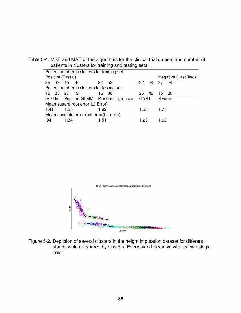
Table 5-4. MSE and MAE of the algorithms for the clinical trial dataset and number ofpatients in clusters for training and testing sets.
Patient number in clusters for training setPositive (First 8) Negative (Last Two)26 39 15 28 22 53 32 24 37 24Patient number in clusters for testing set19 33 27 19 16 38 26 42 15 30iHGLM Poisson GLMM Poisson regression CART RForestMean square root error(L2 Error)1.41 1.58 1.92 1.65 1.75Mean absolute error root error(L1 error).94 1.34 1.51 1.23 1.62
Diamater
Hei
ght
Plot Of Height−Diamaters, Regression Clusters and Estimates
Figure 5-2. Depiction of several clusters in the height imputation dataset for differentstands which is shared by clusters. Every stand is shown with its own singlecolor.
86

CHAPTER 6DENOISING TIME SERIES BY WAY OF A FLEXIBLE MODEL FOR PHASE SPACE
RECONSTRUCTION
In this chapter, we have used the Dirichlet Process mixtures of linear regression for
solving the time series denoising problem.
Time Delay Embedding and False Neighborhood Method
Time delay embedding has become a common approach to reconstruct the phase
space from an experimental time series. The central idea is that the dynamics is
considered to be governed by a solution traveling through a phase space and a smooth
function maps points in the phase space to the measurement with some error. Given a
time series of measurements, x(1), x(2), ...., x(N), the phase space is represented by
vectors in D-dimensional euclidean space.
y (n) = ⟨x (n) , x (n + T ) , ....., x (n + (D − 1)T )⟩ (6–1)
Here, T is the time delay and D is the embedding dimension. The temporally sub-
sequent point to y (n) in the phase space is y (n + 1). The purpose of the embedding is
to unfold the phase space to a multivariate space, which is representative of the original
dynamics. Takens (1981) has shown that under suitable conditions, if the dynamical
system has dimension dA and if the embedding dimension is chosen as D > 2dA, then
all the self-crossings in the trajectory due to the projection can be eliminated. The false
neighborhood method Kennel et al. (1992) accomplishes this task, where it views the
dynamics as a compact object in the phase space. If the embedding dimension is too
low (the system is not correctly unfolded), many points that lie very close to each other
(i.e., neighbors) are far apart in the higher dimensional correctly unfolded space. Iden-
tification of these false neighbors allows the technique to determine that the dynamical
system has not been correctly unfolded.
For, the time series, x(n), in d th and (d+1)th dimensional embedding, the Euclidean
distance between an arbitrary point, y(n) and its closest neighbor y FL(n) is, R2d (n) =
87

∑d−1k=0[x(n + kT ) − x FL(n + kT )]2 and R2
d+1(n) =∑d
k=0[x(n + kT ) − x FL(n + kT )]2
respectively. If the ratio of these two distances exceeds a threshold Rtol (we took this
as 15 in this dissertation), the points are considered to be false neighbors in the d th
dimension. The method starts from d = 1 and increases it to D, until only 1 − 2%
of the total points appear as false neighbors. Then, we deem the phase space to be
completely unfolded in RD , a D-dimensional Euclidean Space.
NPB-NR Model
Step One: Clustering of Phase Space
Given a time series {x (1) , x (2) , ..x (N)}, let the minimum embedding dimension be
D (using the False Neighborhood). Hence, the reconstructed phase space is,
x(1) x(2) ... x(N − (D − 1)T )
x(1 + T ) x(2 + T ) ... x(N − (D − 2)T )
...... . . . ...
x(1 + (D − 1)T ) x(2 + (D − 1)T ) ... x(N)
(6–2)
Here, each column represents a point in the phase space. The generative model of
the points in the phase space is now assumed as,
βi |α1,α2 ∼ Beta(α1,α2), {µi ,d ,λi ,d} ∼ N(µi ,d |md , (βd ,λi ,d)
−1)Gamma (λi ,d |ad , bd)
zn| {v1, v2, .....} ∼ Categorical {π1,π2,π3....} , Xd (n) |zn ∼ N (µzn,d ,λzn,d)
(6–3)
Here, Xd (n) is the d th co-ordinate of the nth phase space point. {z , v ,µi ,d ,λi ,d} is
the set of latent variables. The distribution, {µi ,d ,λi ,d}, is the base distribution of the
DP. {π1,π2,π3....} denotes the categorical distribution parameters. In this DP mixture,
the sequence, {M1,M2,M3....}, creates an infinite vector of mixing proportions and
{µzn,d ,λzn,d} are the atoms representing the mixture components. This infinite mixtures
of Gaussians picks clusters for each phase space point and lets the phase space
88

data determine the number of clusters. From this perspective, we can interpret the DP
mixture as a flexible mixture model in which the number of components (i.e., the number
of cells in the partition) is random and grows as new data is observed.
Step Two: Nonlinear Mapping of Phase Space Points
Due to the discretization of the original continuous phase space, our assumption is
that a point in the phase space is constructed by a nonlinear map R whose form we wish
to approximate. In this section, we approximate this nonlinear map of the subsequent
phase space points via the proposed nonlinear regression. We assume that a specific
cluster has N points. We reorder these points according to their occurrence in the time
series. We then pick the corresponding image of these points (which are the temporally
subsequent phase space points according to the original time delay embedding). We
map each phase space points in the cluster through an infinite mixtures of Linear
Regression to their respective images. The model is formally defined as:
y1 (n) = R1 (x (n)) y2 (n) = R2 (x (n)) ....yD (n) = RD (x (n)) (6–4)
Here, R1:D are nonlinear Regressors which is described by the following set of
equations. Here, Xd (n) and Y1 (n) represent the d th co-ordinate of the nth phase space
point and the first co-ordinate of its post image respectively. {z , v ,µi ,d ,λx ,i ,d , βi ,d ,λy ,i} is
the set of latent variables and the distributions, {µi ,d ,λx ,i ,d} and {βi ,d ,λy ,i} are the base
distributions of the DP. {π1,π2,π3, ...}. Although these set of equations are for R1, the
same model applies for R2:D , representing Y2:D (n).
βi |α1,α2 ∼ Beta(α1,α2), {βi ,d ,λy ,i} ∼ N(βi ,d |my ,d , (βy ,λy ,i)
−1)Gamma (λy ,i |ay , by)
zn| {β1, β2, .....} ∼ Categorical {π1,π2,π3....} ,
Y1 (n) |X (n) , zn ∼ N(βzn,0 +
∑D
d=1 βzn,dXd (n) ,λ−1y ,zn
)(6–5)
89

The infinite mixture model approach to the Linear Regression makes the covariates
be associated with the model via a nonlinear function, resulting from marginalizing over
the other mixtures with respect to a specific mixture. Also, now the variance is different
across different mixtures, thereby capturing Heteroscedasticity.
Step Three: Restructuring of the Dynamics
The idea here is to perturb the trajectory to make the modified phase space more
consistent with the dynamics, which is equivalent to reducing the error by perturbing the
phase space points from its original position and also the error between the perturbed
position and the mapped position. We have to choose a new sequence of phase space
points, x (n), such that following objective is minimized.
∑N
n=1(∥x (n)− x (n)∥2 + ∥x (n)− R(
xpre−image)∥2 + ∥R
(x (n)
)−(
xpost−image)∥2 (6–6)
R is the nonlinear Regressors (R1:D) that are used to temporally approximate the
phase space (Described in the section above). N is the number of points in the specific
cluster. This is done across all the clusters. In addition, to create the new noise removed
time series, perturbations of xd (n)’s are done consistently for all subsequent points,
such that we can revert back from the phase space to a time series. For example, if
the time delay is 1 and the embedding dimension is 2, then, the phase space points
are perturbed in such a way that when x (n) = (t(n), t(n + 1)) is moved to x (n) =(t(n), t(n + 1)
), we make the first co-ordinate of x (n + 1) to be t (n + 1). These form
a set of equality constraints. What results is a convex program, that is then solved to
retrieve the denoised time series.
The entire algorithm is summarized in Table 6-1.
90

Table 6-1. Step-wise description of NPB-NR process.1. Form the phase space dynamics from the noisy time serieswith the embedding dimension determined by false neighbor-hood method.2. Cluster the points in the phase space via infinite mixture ofGaussian densities.3. For each cluster, map each phase space point via an infinitemixtures of linear regression(R1:D) to its temporally subsequentpoint (post-image).4. Infer the latent parameters for both infinite mixture ofGaussian densities and infinite mixture of linear regression.{z , v ,µi ,d ,λi ,d} and {z , v ,µi ,d ,λx ,i ,d , βi ,d ,λy ,i} were inferredthrough variational inference. The inference gives us the form ofthe regressors,(R1:D).5. Restructure the dynamics via optimizing the Convex function.The restructuring is done consistently for all the subsequentpoints, which leads to the reconstruction of the noise removedtime series.
Experimental Results
An Illustrative Description of the NPB-NR Process
First, we present an illustrative pictorial description of the complete NPB-NR pro-
cess with a real world historical stock price dataset. Our model for the historical time
series of the stock price is a low-dimensional dynamical system that was contaminated
by noise and passed through a measurement function at the output. Our task was to
denoise the stock price to not only recover the underlying original phase space dynam-
ics and create the subsequent noise removed stock price via the NPB-NR process,
but also to utilize it to make better future predictions of the stock price. We picked
historical daily close out stock price data of IBM from March-1990 to Sept-2015 for
this task. The original noisy time series is plotted in Figure 6-1. The various stages
of NPB-NR are illustrated in the subsequent figures. The underlying dimension of the
phase space turned out to be 3 from the False Neighborhood Method. The Recon-
structed Phase Space with noise is shown in Figure 6-2. The completely clustered
phase space and one specific cluster in the phase space by Dirichlet Process Mixture
91
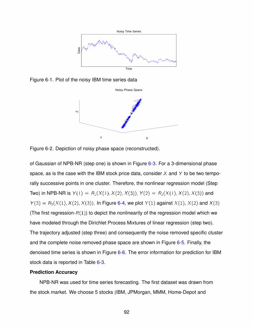
Noisy Time Series
Time
Dat
aFigure 6-1. Plot of the noisy IBM time series data
X
Noisy Phase Space
Y
Z
Figure 6-2. Depiction of noisy phase space (reconstructed).
of Gaussian of NPB-NR (step one) is shown in Figure 6-3. For a 3-dimensional phase
space, as is the case with the IBM stock price data, consider X and Y to be two tempo-
rally successive points in one cluster. Therefore, the nonlinear regression model (Step
Two) in NPB-NR is Y (1) = R1(X (1),X (2),X (3)),Y (2) = R2(X (1),X (2),X (3)) and
Y (3) = R3(X (1),X (2),X (3)). In Figure 6-4, we plot Y (1) against X (1), X (2) and X (3)
(The first regression-R(1)) to depict the nonlinearity of the regression model which we
have modeled through the Dirichlet Process Mixtures of linear regression (step two).
The trajectory adjusted (step three) and consequently the noise removed specific cluster
and the complete noise removed phase space are shown in Figure 6-5. Finally, the
denoised time series is shown in Figure 6-6. The error information for prediction for IBM
stock data is reported in Table 6-3.
Prediction Accuracy
NPB-NR was used for time series forecasting. The first dataset was drawn from
the stock market. We choose 5 stocks (IBM, JPMorgan, MMM, Home-Depot and
92

X
Phase Space with the clusters
YZ
X
Plot of One Specific Cluster
Y
Z
Figure 6-3. Depiction of whole clustered phase space (step one) and one single cluster
Y(1) with covariate X(1)
X(1)
Y(1
)
Y(1) with covariate X(2)
X(2)
Y(1
)Y(1) with covariate X(3)
X(3)
Y(1
)Figure 6-4. Regression data: Y(1) regressed with covariate as X(1), X(2) and X(3)
X
Noise Removed Cluster
Y
Y
X
Noise Removed Phase Space
Y
Y
Figure 6-5. Single noise removed cluster and whole noise removed phase space
Noise Removed Time Series
Time
Dat
a
Figure 6-6. Plot of the noise removed time series data
93

Walmart) from March, 2000 to Sept., 2015 with 3239 instances (time points) from
“DOW30”. The next four datasets came from the Santa Fe competition compiled in
Gershenfeld and Weigend (1994). The first is a Laser generated dataset which is a
univariate time record of a single observed quantity, measured in a physics laboratory
experiment. The next is a Currency Exchange Rate Dataset which is a collection of
tickwise bids for the exchange rate from Swiss Francs to US Dollars, from August 1990
to April 1991. The next dataset is a synthetic computer generated series governed by
a long sequence of known high dimensional dynamics. The fourth dataset is a set of
astrophysical measurements of light curve of the variable white dwarf star PG 1159035
in March, 1989. The next set of datasets are the Darwin sea level pressure dataset
from 1882 to 1998, Oxygen Isotope ratio dataset of 2.3 million years and US Industrial
Production Indices dataset from Federal Reserve release. NPB-NR was compared with
the GARCH, AR (ρ), ARMA (p, q) and ARIMA (p, d , q) models, where ρ, p, d , q were
taken by cross-validations ranging from 1 to 10 fold. We also compared NPB-NR to PCA
and kernel PCA Bishop (2006) with sigma set to 1, and Gaussian Process Based Auto-
regression with ρ taken by cross-validations ranging from 1 to 5 fold. We also compared
results from Hard Threshold Wavelet denoising using the “wden” Matlab function. All
competitor algorithms were run with a 50-50 training-testing split. We report the Mean
Square Error (MSE, L2) of the forecast for all the competitor algorithms in Table 6-
3. Individual time series were reconstructed into a phase space with the dimension
determined by the False Neighborhood method, was passed through NPB-NR to find
the most consistent dynamics by reducing noise, and subsequently fed into a simple
auto-regressor with lag order taken as the embedding dimension of the reconstructed
time series. In most datasets, NPB-NR not only yielded better forecasts, but also a
smaller standard deviation among its competitors among the 10 runs.
94

Noise Reduction Experiment
We evaluated the NPB-NR technique for noise reduction across several well known
dynamical systems, namely, Lorenz attractor (chaotic) Lorenz (1963), Van-der-poll
attractor Pol (1920) and Rossler attractor Rossler (1976) (periodic), Buckling Column
attractor (non strange non chaotic, fixed point), Rayleigh attractor (non strange non
chaotic, limit cycle) Abraham and Shaw (1985) and GOPY attractor (strange nonchaotic)
Grebogi et al. (1984).
Although noise was added to the time series such that the SNR ranged from 15
db to 100 db, it is impossible to calculate numerically or from the Power Spectrum how
much noise was actually removed from the noisy time series. Therefore, for both the
noise removed and the noisy time series we calculated the fluctuation error:,
fi = ∥xi − xi−1 − (dt) · f (xi−1, yi−1, zi−1)∥
This measures the distance between the observed and the predicted point in the
phase space. Here, measurement of the noise reduction percentage is given by,
R = 1− Enoise−removed
Enoisy, E =
(∑f 2i
N
) 12
We tabulated the noise reduction percentages of the NPB-NR, the low pass filter,
and also wavelet denoising methods in Table 6-4. For the wavelet method, we used the
matlab “wden” function in ’soft’ and ’hard’ threshold mode. The NPB-NR yielded the
highest noise reduction percentage for 15-100 db SNR. Since the faithful reconstruction
of the underlying dynamics intrinsically removes the noise, as the noise increases the
noise reduction performance of NPB-NR got significantly better as opposed to the other
techniques.
Power Spectrum Experiment
We ran a Power Spectrum experiment for a noise corrupted Van-der-poll attractor
(periodic) Pol (1920) as well as a time series created by superimposing 6 Sinusoids and
95

0 10 20 30 40 50−60
−40
−20PSD−Noisy
Frequency (Hz)
Ma
gn
itu
de
(D
B)
0 10 20 30 40 50−100
−50
0PSD−NPB−NR
Frequency (Hz)
Ma
gn
itu
de
(D
B)
0 10 20 30 40 50−100
−50
0PSD−Low−Pass−Filter
Frequency (Hz)
Ma
gn
itu
de
(D
B)
0 10 20 30 40 50−100
−50
0PSD−OLS
Frequency (Hz)
Ma
gn
itu
de
(D
B)
Phase Space−Noisy
X1
Y1
Phase Space−NPB−NR
X1
Y1
Phase Space−Low−Pass−Filter
X1
Y1
Phase Space−OLS
X1
Y1
0 500 1000 1500−60
−40
−20PSD−Noisy
Frequency (Hz)
Ma
gn
itu
de
(D
B)
0 500 1000 1500−100
−50
0PSD−NPB−NR
Frequency (Hz)
Ma
gn
itu
de
(D
B)
0 500 1000 1500−100
−50
0PSD−Low−Pass−Filter
Frequency (Hz)M
ag
nitu
de
(D
B)
0 500 1000 1500−100
−50
0PSD−OLS
Frequency (Hz)
Ma
gn
itu
de
(D
B)
X
Phase Space−Noisy
Y
Z
X
Phase Space−NPB−NR
Y
Z
X
Phase Space−Low−Pass−Filter
Y
Z
X
Phase Space−OLS
Y
Z
Figure 6-7. Power spectrum and phase space plot of Van-der-poll and sinusoid attractor
subsequently corrupting it with noise. The noise was additive white Gaussian noise with
the SNR (Signal-to-Noise ratio) set at 15 db. Var-der-poll is a simple two dimensional
attractor with b = 0.4; x0 = 1; y0 = 1 and the superimposition of Sinusoids is a simple
limit cycle attractor with negative Lyapunov Exponents and no fractal structure. We plot
the phase space and the Power Spectrum of the noisy time series generated from these
attractors, the noise removed solution with a 6th-order Butterworth low-pass filter (cut-off
freq. 30 Hz and 1000 Hz respectively) and the NPB-NR technique. The Power Spectrum
and the phase space plot of the Van-der-poll and Sinusoid attractors is shown in Figure
6-7. Note that NPB-NR successfully made the harmonics/peaks more prominent which
was originally obscured by the noise. The filtering method was unable to restore the
harmonics, although it removed some of the higher frequency components. We also
96

observe that NPB-NR smoothened out the phase space dynamics better than the low
pass filter.
Experiment with Dimensions
We can view noise as high-dimensional dynamics which is added to the low-
dimensional attractor. Therefore, noise kicks up the dimension of the resulting dynamics.
We evaluated the NPB-NR method to check whether it brings down the dimension to the
original desired dimension of the attractor. We first calculated the minimum embedding
dimension (when False Neighborhood Percentage falls below 1%). Then we passed
each time series though NPB-NR. After this, we evaluated the minimum embedding
dimension again for the newly created noise removed time series. We found that NPB-
NR significantly outperforms the low-pass filtering technique to bring down the minimum
embedding dimension of the underlying attractor to the original. We have also compared
NPB-NR against traditional dimensionality reduction techniques like PCA and kernel
PCA with sigma set as 1. For PCA and kernel PCA, we set the original dimension
as 15 for all the attractors. Then, the underlying dimension was determined as when
the cumulative variance of the top eigen-vectors rose above 98%. Numerical results
show that PCA or kernel PCA cannot find the correct underlying dimension of the noisy
attractors. The reason behind this is that the goal of PCA/kernel PCA is to project the
higher dimensional data to the lower dimensional subspace with maximum spread. In
the presence of noise, without being tied to the model of the dynamics, PCA/Kernel
PCA distorts the dynamics severely and retrieves a dimension entirely different from
the original. If the underlying dimension picked is lower than the original, it is unable to
unfold the attractor. If greater, there is enough residual noise to degrade the prediction
accuracy. All the experiments in this section were done under 15 db SNR.
s
97

Table 6-2. Minimum embedding dimension of the attractors with their original dimension,dimension of noisy time series and dimension of noise removed time serieswith the NPB-NR, low pass filter, PCA and KERNEL-PCA.
Lorenz GOPY Van-Der-Poll Rossler RayleighOriginal dimension 3 2 2 3 2Dimension-noisy 8 7 7 10 5Noise removed dimensionNPB-NR 4 2 2 3 3Low pass filter 6 5 5 4 4PCA 5 3 4 5 4KERNEL-PCA 2 3 3 4 4
Table 6-3. MSE and standard deviation of all the datasets for all the competitoralgorithms in 50-50 random training-testing split for 10 runs.
MSE NPB-NR GARCH Wavelet AR ARMA ARIMA PCA KERNEL-PCA GPRIBM 1.43 1.65 1.37 1.87 1.70 1.68 1.98 1.90 1.84JPM 1.38 1.52 1.49 1.46 1.42 1.39 1.67 1.59 1.73MMM 1.69 1.87 1.96 2.06 1.93 1.83 1.14 2.11 2.23HD 1.74 1.58 1.46 1.73 1.69 1.62 1.79 1.72 1.86WMT 1.24 1.47 1.58 1.39 1.35 1.29 1.49 1.57 1.38LASER .97 1.36 1.29 1.31 .86 1.15 1.42 1.35 1.34CER .82 .99 .93 .94 .88 .84 1.18 1.11 1.05CGS 1.79 2.11 1.88 2.03 1.96 1.86 2.38 2.28 2.17ASTRO 1.82 2.19 2.14 2.08 1.91 1.92 2.26 2.33 2.46DSLP 1.33 1.68 1.53 1.49 1.41 1.14 1.68 1.60 1.55OxIso 1.19 1.38 1.87 1.32 1.26 1.53 1.48 1.41 1.45USIPI 1.30 1.57 1.36 1.48 1.43 1.62 1.57 1.57 1.63Stan. dev. NPB-NR GARCH Wavelet AR ARMA ARIMA PCA KERNEL-PCA GPRIBM 1.34 1.89 1.86 1.67 1.78 1.39 3.26 2.37 1.42JPM 1.63 1.98 1.97 1.78 1.94 2.01 2.35 1.69 2.21MMM 1.82 1.48 1.29 1.42 1.36 1.82 1.73 1.66 1.59HD 1.86 1.85 1.85 1.92 1.77 1.88 1.93 1.90 1.86WMT 1.79 1.66 1.82 1.62 1.73 2.31 1.67 1.61 1.98LASER 2.12 2.28 2.39 2.19 2.36 1.72 2.42 2.27 2.39CER 1.69 1.78 1.93 1.84 1.74 1.71 1.80 1.91 1.72CGS 2.34 1.92 1.88 1.97 2.05 1.87 1.95 2.17 2.11ASTRO 1.13 1.82 1.41 1.37 1.69 1.79 1.55 1.29 1.62DSLP 1.58 1.49 1.19 1.27 1.35 1.45 1.26 1.42 1.25OxIso 2.47 2.15 1.99 2.24 1.89 2.25 1.92 2.61 2.45USIPI 2.23 2.33 2.49 2.42 1.89 2.29 2.37 2.72 2.25
98

Table 6-4. Noise reduction percentage of the attractors for the NPB-NR, the low passfiltering method and the hard and soft threshold wavelet method.
Lorenz GOPY Van-Der-Poll Rossler RayleighNoise level–15db SNRNPB-NR 40 45 54 29 34Low pass filter 19 27 40 19 31Wavelet soft 15 13 29 21 25Wavelet hard 17 7 21 18 22Noise level–35db SNRNPB-NR 51 59 61 40 56Low pass filter 26 31 40 28 39Wavelet soft 22 22 36 33 32Wavelet hard 23 14 29 24 28Noise level–60db SNRNPB-NR 63 71 75 79 82Low pass filter 31 35 40 37 41Wavelet soft 32 29 41 40 42Wavelet hard 29 21 33 32 33Noise level–80db SNRNPB-NR 72 76 79 81 84Low pass filter 34 39 43 43 44Wavelet soft 35 35 46 44 47Wavelet hard 34 27 39 36 38Noise level–100db SNRNPB-NR 80 79 85 85 89Low pass filter 38 43 46 47 46Wavelet soft 41 39 50 50 60Wavelet hard 36 30 45 40 51
99

CHAPTER 7CONCLUSION AND FUTURE WORK
In the first part, we have formulated infinite mixtures various GLM models via a
stick breaking prior as hierarchical Bayesian graphical models. We have derived fast
mean field variational inference algorithms for each of the models. The algorithms are
particularly useful for high dimensional datasets where Gibbs sampling fails to scale
and is slow to converge. The algorithms have been tested successfully on four datasets
against their well known competitor algorithms across many settings of training/testing
splits.
In the next part, we have formulated an infinite multigroup Generalized Linear Model
(iMG-GLM), a flexible model for shared learning among groups in grouped regression.
The model clusters groups by identifying identical response-covariate densities for
different groups. We experimentally evaluated the model on a wide range of problems
where traditional mixed effect models and group specific regression models fail to
capture structure in the grouped data.
In the third part, we have formulated an infinite mixtures of Hierarchical Generalized
Linear Model (iHGLM), a flexible model for hierarchical regression. The model captures
identical response-covariate densities in different groups as well as different densities in
the same group. It also captures heteroscedasticity and overdispersion across groups.
We experimentally evaluated it on a wide range of problems where traditional mixed
effect models fail to capture structure in the grouped data.
In the final part, we have formulated a Bayesian nonparametric model for noise
reduction in time series. The model captures the local nonlinear dynamics in the time
delay embedded phase space to fit the most appropriate dynamics consistent with
the data. Finally, we have evaluated the NPB-NR technique on various time series
generated from several dynamical systems, stock market data, LASER data, sea level
pressure data, etc. The technique yields much better noise reduction percentage, power
100

spectrum analysis, accurate dimension and prediction accuracy. In the experiments, we
varied the scale factor which modulates the number of clusters in the phase space.
While the variational methods for GLM models, developed in a mean field setting,
it would be worth exploring other variational methods in the non-parametric Bayesian
context to the Generalized Linear Models. For the multigroup and multilevel regressions,
although the Gibbs sampler turned out to be fairly accurate for the iMG-GLM and iHGLM
models, developing a variational inference alternative would be an interesting topic for
future research. Finally, the number of mixture components in each group depends
on the scale factors γ and α (scale parameters of the DP and HDP) of the model, and
at times grows large in specific groups. This occurs mostly when any group has a
large number of data points compared to others. In most cases, beyond a few primary
clusters, the remaining represent outliers. Although, careful tuning of scale parameters
can mitigate these problems, a theoretical understanding of the dependence of the
model on scale parameters could lead to better modeling and application. Although,
the Metropolis Hastings algorithm turned out to be fairly accurate for the iMG-GLM-2
model, developing a variational inference alternative would be an interesting topic for
future research. For the final part, we plan to explore which kind of physical systems
can be analyzed using nonparametric Bayesian based noise reduction methods. Finally,
considerable effort should be given to analyzing time series generated from higher
dimensional systems.
101

REFERENCES
A. Tsanas, P. E. McSharry, M. A. Little and Ramig, L. O. “Accurate Telemonitoring ofParkinsons Disease Progression by Non-invasive Speech Tests.” IEEE transactionson Biomedical Engineering 57 (2009): 884–893.
Abraham, R. and Shaw, C. Dynamics: The Geometry of Behavior. Ariel Press, 1985.
Ando, Rie Kubota and Zhang, Tong. “A Framework for Learning Predictive Structuresfrom Multiple Tasks and Unlabeled Data.” Journal of Machine Learning Research 6(2005): 1817–1853.
Antoniak, C. E. “Mixtures of Dirichlet Processes with Applications to Bayesian Nonpara-metric Problems.” Annals of Statistics 2 (1974).6: 1152–1174.
Badii, R., Broggi, G., Derighetti, B., Ravani, M., Ciliberto, S., Politi, A., and Rubio, M.A.“Dimension increase in filtered chaotic signals.” Phys. Rev. Lett. 60 (1988): 979–982.
Bakker, B. and Heskes, T. “Task Clustering and Gating for Bayesian Multitask Learning.”Journal of Machine Learning Research 4 (2003): 83–99.
Baxter, Jonathan. “Learning Internal Representations.” International Conference onComputational Learning Theory (1995): 311–320.
———. “A Model of Inductive Bias Learning.” Journal of Artificial Intelligence Research12 (2000): 149–198.
Bishop, C. M. Pattern Recognition and Machine Learning. Springer-Verlag, 2006.
Blackwell, D. and MacQueen, J. B. “Ferguson Distributions Via Polya Urn Schemes.”Annals of Statistics 1 (1973).2: 353–355.
Blei, D. and Jordan, M. “Variational Inference for Dirichlet Process Mixtures.” BayesianAnalysis 1 (2006): 121–144.
Breslow, N. E. and Clayton, D. G. “Approximate Inference in Generalized Linear MixedModels.” Journal of the American Statistical Association 88 (1993).421: 9–25.
Caruana, Rich. “Multitask Learning.” Machine Learning 28 (1997).1: 41–75.
Cortes, C. and Vapnik, V. “Support Vector Networks.” Machine Learning 20 (1995):273–297.
D. Blei, A. Ng and Jordan, M. “Latent Dirichlet Allocation.” Journal of Machine LearningResearch 3 (2003): 993–1022.
David, L. and Donoho, J. “De-noising by Soft-thresholding.” IEEE Trans. Inf. Theor. 41(1995).3: 613–627.
102

Elshorbagy, A. and Panu, U.S. “Noise reduction in chaotic hydrologic time series: factsand doubts.” Journal of Hydrology 256 (2002).34: 147–165.
Escobar, D. M. and West, M. “Bayesian Density Estimation and Inference UsingMixtures.” Journal of the American Statistical Association 90 (1995).430: 577–588.
Ferguson, T.S. “A Bayesian Analysis of Some Nonparametric Problems.” Annals ofStatistics 1 (1973): 209–230.
Gelman, A. and Wolberg, D. B. Rubin. “Inference From Iterative Simulation usingMultiple Sequences.” Statistical Sciences 7 (1992): 457–511.
Gershenfeld, N. and Weigend, A. Time Series Prediction: Forecasting the Future andUnderstanding the Past. Addison-Wesley, 1994.
Ghahramani, Z. and Beal, M. “Propagation Algorithms for Variational Bayesian Learn-ing.” Proceedings of 13th Advances in Neural Information Processing Systems (2000):507–513.
Grassberger, P., Schreiber, T., and Schaffrath, C. “Non-linear time sequence analysis.”International Journal of Bifurcation and Chaos 1 (1991).3: 521–547.
Grebogi, C., Ott, E., Pelikan, S., and Yorke, J. A. “Strange attractors that are not chaotic.”Physica D: Nonlinear Phenomena 13 (1984).1: 261–268.
Hannah, L., Blei, D., and Powell, W. “Dirichlet Process Mixtures of Generalized LinearModels.” Journal of Machine Learning Research 12 (2011): 1923–1953.
Hastie, T. and Tibshirani, R. “Varying-Coefficient Models.” Journal of the Royal StatisticalSociety. Series B (Methodological) 55 (1993).4: 757–796.
IBM. “IBM Spss Version 20.” IBM SPSS SOFTWARE (2011).
Ishwaran, H. and James, L. F. “Gibbs Sampling Methods for Stick-Breaking Priors.”Journal of the American Statistical Association 96 (2001).453: 161–173.
Jordan, M. and Jacobs, R. “Hierarchical mixtures of experts and the EM algorithm.”International Joint Conference on Neural Networks (1993).
Kennel, Matthew B., Brown, Reggie, and Abarbanel, Henry D. I. “Determining embed-ding dimension for phase-space reconstruction using a geometrical construction.”Phys. Rev. A 45 (1992).6: 3403–3411.
Kostelich, E. J. and Yorke, J. A. “Noise Reduction: Finding the Simplest DynamicalSystem Consistent with the Data.” Phys. D 41 (1990).2: 183–196.
Lee, Y. and Nelder, J. A. “Hierarchical Generalized Linear Models.” Journal of the RoyalStatistical Society. Series B (Methodological) 58 (1996).4: 619–678.
103

———. “Hierarchical Generalised Linear Models: A Synthesis of Generalised LinearModels, Random-Effect Models and Structured Dispersions.” Biometrika 88 (2001a).4:987–1006.
———. “Modelling and analysing correlated non-normal data.” Statistical Modelling 1(2001b).1: 3–16.
———. “Double hierarchical generalized linear models (with discussion).” Journal of theRoyal Statistical Society: Series C (Applied Statistics) 55 (2006).2: 139–185.
Lorenz, E. N. “Deterministic Nonperiodic Flow.” Journal of the Atmospheric Sciences 20(1963).2: 130–141.
Lowd, D. and Domingos, P. “Naive Bayes models for probability estimation.” Proceedingsof the 22nd international conference on Machine learning (2005): 529–536.
M. Jordan, T. Jaakkola, Z. Ghahramani and Saul, L. “Introduction to Variational Methodsfor Graphical Models.” Machine Learning 37 (2001): 183–233.
Mallat, S. and Hwang, W. L. “Singularity detection and processing with wavelets.”Information Theory, IEEE Transactions on 38 (1992).2: 617–643.
Mitschke, F., Moller, M., and Lange, W. “Measuring filtered chaotic signals.” Phys. Rev. A37 (1988).11: 4518–4521.
Neal, R. M. “Markov Chain Sampling Methods for Dirichlet Process Mixture Models.”Journal of Computational and Graphical Statistics 9 (2000a).2: 249–265.
———. “Markov Chain Sampling Methods for Dirichlet Process Mixture Models.” Journalof Computational and Graphical Statistics 9 (2000b).2: 249–265.
Nelder, J. A. and Wedderburn, R. W. M. “Generalized Linear Models.” Journal of theRoyal Statistical Society, Series A (General) 135 (1972).3: 370–384.
Pol, B. V. D. “A theory of the amplitude of free and forced triode vibrations.” RadioReview 1 (1920): 701–710.
Rasmussen, C. E. and Williams, C.K.I. “Gaussian Processes for Machine Learning(Adaptive Computation and Machine Learning).” MIT Press (2005a).
Rasmussen, C.E. and Williams, C.K.I. Gaussian Processes for Machine Learning(Adaptive Computation and Machine Learning). MIT Press, 2005b.
Robert, C. and Casella, G. Monte Carlo Statistical Methods. Springer-Verlag, 2001.
Robert, C.P. and Casella, G. Monte Carlo Statistical Methods (Springer Texts inStatistics). Springer-Verlag New York, Inc., 2005.
104

Robinson, A. P. and Wykoff, W. R. “Imputing missing height measures using a mixed-effects modeling strategy.” Canadian Journal of Forest Research 34 (2004): 2492–2500.
Rossler, O.E. “An equation for continuous chaos.” Physics Letters A 57 (1976).5:397–398.
S. Ghosal, J. K. Ghosh and Ramamoorthi, R. V. “Posterior consistency of Dirichletmixtures in density estimation.” Annals of Statistics 27 (1999): 143–158.
Schwartz, L. “On Bayes procedures.” Zeitschrift fr Wahrscheinlichkeitstheorie undVerwandte Gebiete 4 (1965).1: 10–26.
Sethuraman, J. “A Constructive Definition of Dirichlet Priors.” Statistica Sinica 4 (1994):639–650.
Site, G. and Ramakrishnan, A. G. “Wavelet domain nonlinear filtering for evokedpotential signal enhancement.” Computer and Biomedical Research 33 (2000).3:431–446.
Takens, Floris. “Dynamical Systems and Turbulence, Warwick 1980.” Detecting strangeattractors in turbulence 898 (1981): 366–381.
Teh, Y. W., Jordan, M. I., Beal, M., and Blei, D. “Hierarchical Dirichlet Processes.”Journal of the American Statistical Association 101 (2006): 1566–1581.
Tokdar, S. T. “Posterior Consistency of Dirichlet Location-Scale Mixture of Normals inDensity Estimation and Regression.” Sankhya: The Indian Journal of Statistics 68(2006).1: 90–110.
Viele, K. and Tong, B. “Modeling with Mixtures of Linear Regressions.” Statistics andComputing 12 (2002).4: 315–330.
Wang, Zidong, Lam, James, and Liu, Xiaohui. “Filtering for a class of nonlinear discrete-time stochastic systems with state delays.” Journal of Computational and AppliedMathematics 201 (2007).1: 153–163.
Wolberg, W.H. and Mangasarian, O. L. “Multisurface method of pattern separation formedical diagnosis applied to breast cytology.” Proceedings of the National Academyof Sciences 87 (1990): 9193–9196.
Y. W. Teh, M. J. Beal, M. I. Jordan and Blei, D. M. “Hierarchical Dirichlet Processes.”Journal of the American Statistical Association 101 (2006): 1566–1581.
Ya Xue, Xuejun Liao and Carin, Lawrence. “Multi-task Learning for Classification withDirichlet Process Priors.” Journal of Machine Learning Research 8 (2007): 35–63.
Yu, Kai, Tresp, Volker, and Schwaighofer, Anton. “Learning Gaussian Processes fromMultiple Tasks.” International Conference on Machine Learning (2005): 1012–1019.
105

Zhang, Jian, Ghahramani, Zoubin, and Yang, Yiming. “Learning Multiple Related Tasksusing Latent Independent Component Analysis.” Advances in Neural InformationProcessing Systems (2005): 1585–1592.
Zhang, L., Bao, P., and Pan, Q. “Threshold analysis in wavelet-based denoising.”Electronics Letters 37 (2001).24: 1485–1486.
106

BIOGRAPHICAL SKETCH
Minhazul Islam Sk was born at the small town of Burdwan of West Bengal province
in India. After finishing his high school in Burdwan C.M.S. high school, he was admitted
to Jadavpur University in Kolkata for his undergraduate studies in Electronics And
Telecommunication Engineering in 2008. After finishing his undergraduate education in
2012, he was admitted to the Ph.D. program in the Computer and Information Science
and Engineering Department at the University of Florida in Gainesville, Florida, USA in
2012. His primary area of research is machine learning and applied statistics especially
in the area of regression and Bayesian nonparametrics. He graduated with a Ph.D. from
the University of Florida in August 2017.
107


![Reactor Physics: Multigroup Diffusion · Reactor Physics: Multigroup Diffusion 6 This work is detailed in [GARLAND1975] but for the present discussion, the main point to note is the](https://img.dokumen.tips/doc/110x75/5e38d3c86fdaec5c757d1316/reactor-physics-multigroup-reactor-physics-multigroup-diffusion-6-this-work-is.jpg)