Embed Size (px)
Citation preview

AUTOMATIC CONTROL
Exercises
Department of Automatic Control
Lund University, Faculty of Engineering
June 2017
1


1. Model Building and Linearization
1.1 Many everyday situations may be described and analyzed using con-cepts from automatic control. Analyze the scenarios below and try togive a description that captures the relevant properties of the system:
• What should be controlled?
• What control signals are used?
• What measurement signals are available?
• Is the system affected by any disturbances?
• Is feedback or feedforward used for control?
• Draw a block diagram that describes the system. The block dia-gram should show how the measurement signals, control signals,and the disturbances are connected to the human (which here isthe controller), and to the process.
a. You take a shower and try to get desired temperature and flow of thewater.
b. You drive a car.
c. You boil potatoes on the stove.
1.2 A car drives on a flat road and we assume that friction and airresistance are negligible. We want to study how the car is affected bythe gas pedal position u. We assume that u varies between 0 and 1,and that the acceleration of the car is proportional to the gas pedalposition, a = ku.
u yBil
a. Write down the differential equation that describes the relation be-tween the gas pedal position u and the velocity v of the car.
b. Let instead the position p of the car be the output signal, y = p.Introduce the states x1 = p and x2 = v, and write the system onstate-space form.
c. Assume that the car is affected by air resistance that gives a counterforce that is proportional to the square of the velocity of the car. Withthe gas pedal position as control signal and the velocity of the car asmeasurement signal, the system may now be written as
x = −mx2 + ku
y = x
The system is no longer linear (why?). Let k = 1 and m = 0.001. Findthe stationary velocity y0 that corresponds to the gas pedal being 10%down, u0 = 0.1.
3

Chapter 1. Model Building and Linearization
d. Linearize the system around the stationary point in c.
1.3
m
k
c
y(t)
f (t)
In the right figure, a mass m is attachedto a wall with a spring and a damper.The spring has a spring constant k andthe damper has a damping constant c. Itis assumed that k > c2/4m. An externalforce f is acting on the mass. We denotethe translation of the mass from its equilibrium position by y. Further,we let f (t) be the input signal and y(t) be the output signal. The forceequation gives
my = −ky− cy+ f
a. Introduce the states x1 = y and x2 = y and write down the statespace representation of the system.
b. Assume that the system is at rest at t = 0 and that f (t) changesfrom 0 to 1 as a step at t = 0. What is the resulting y(t)? Sketch thesolution.
1.4 R
L
Cvin
+
−
vout
+
−
iIn the RLC circuit to the right,the input and output voltages aregiven by vin(t) and vout(t), re-spectively. By means of Kirchhoff’svoltage law we see that
vin − Ri− vout − Ldi
dt= 0
For the capacitor, we additionally have
Cvout = i
Introduce the states x1 = vout and x2 = vout and give the state spacerepresentation of the system.
1.5 qin
qout
h
A cylindrical water tank with cross sectionA has an inflow qin and an outflow qout. Theoutlet area is a. Under the assumption thatthe outlet area is small in comparison tothe cross section of the tank, Torricelli’s lawvout =
√2�h is valid and gives the outflow
rate.
a. What would be a suitable state variable forthis system? Determine a differential equa-tion, which tells how the state variable depends on the inflow qin.
b. Asume that measurement signal y is given by level h. Give a state-space representation of the system.
c. Let the inflow be constant, qin = q0in. Determine the corresponding
constant tank level h0 and outflow q0out. Linearize the system around
this stationary point.
4

Chapter 1. Model Building and Linearization
r(t)
u(t)
Figure 1.1 Satellite orbiting the earth.
1.6 Give the state space representation of the system
...y + 3y+ 2y+ y = u
where u(t) and y(t) are the input and output, respectively. Choosestates x1 = y, x2 = y and x3 = y.
1.7 A process with output y(t) and input u(t) is described by the differ-ential equation
y+√y+ yy = u2
a. Introduce states x1 = y, x2 = y and give the state space representa-tion of the system.
b. Find all stationary points (x01, x0
2, u0) of the system.
c. Linearize the system around the stationary point corresponding tou0 = 1.
1.8 Linearize the system
x1 = x21 x2 +
√2 sin u ( = f1(x1, x2, u))
x2 = x1 x22 +
√2 cos u ( = f2(x1, x2, u))
y = arctanx2
x1+ 2u2 ( = �(x1, x2, u))
around the stationary point u0 =π/4.
1.9 A simple model of a satellite, orbiting the earth, is given by thedifferential equation
r(t) = r(t)ω2 − β
r2(t) + u(t)
where r is the satellite’s distance to the earth and ω is its angularacceleration, see Figure 1.1. The satellite has an engine, which canexert a radial force u.
5

Chapter 1. Model Building and Linearization
a. Introduce the state vector
x(t) =
r(t)r(t)
and write down the nonlinear state space equations for the system.
b. Linearize the state space equations around the stationary point
(
r, r, u)
=(
r0, 0, 0)
Consider r as the output and give the state space representation ofthe linear system. Express r0 in β and ω.
6

2. Dynamical Systems
2.1 A dynamical system may be described in various ways – with a transferfunction, with a differential equation, and with a system of differentialequations on state-space form. In this problem we transfer betweenthe different representations for four examples of dynamical systems,from biology, mechanics, electronics, and economics.
a. A model for bacterial growth in a bioreactor is given by
x =
10 1
−1 −1
x+
0
1
u
y =
1 0
x
where u is the inflow of glucose to the reactor, and y is the biomass. Determine the transfer function from u to y, and a differentialequation that determines the relation between the input and outputsignals of the system.
b. A simple model of a telescope is given by
Jd2y
dt2+ D
dy
dt= u
where yis the angle of the telescope to the earth surface, and u isthe torque from the motor that controls the telescope. Determine thetransfer function from u to y and write the system on state-spaceform.
c. An electronic low pass filter is used at recordings to attenuate highfrequency noise. The input u is the original noisy signal, and theoutput y is the recorded signal. The filter is given on state-space formas
dx
dt= −1
kx+ 1
ku
y = x
Determine the transfer function from u to y.
d. The transfer function for a model that describes economical growth isgiven by
G(s) = γ
s3 +αs2 + βs
where the input u is the difference between savings and investmentsin the economy, and the output y is GDP. Write the system on state-space form.
2.2 Determine the transfer functions and give differential equations, de-scribing the relation between input and output for the following sys-tems, respectively.
7

Chapter 2. Dynamical Systems
a.
x =
−2 0
0 −3
x+
5
2
u
y =
−1 1
x+ 2u
b.
x =
−7 2
−15 4
x+
3
8
u
y =
−2 1
x
c.
x =
−1 0
0 −4
x+
3
2
u
y =
1 0
x+ 5u
d.
x =
1 4
−2 −3
x+
−1
1
u
y =
1 2
x+ 3u
2.3 Determine the impulse and step responses of the systems in assign-ment 2.2.
2.4 Derive the formula G(s) = C(sI − A)−1B+ D for a general system
x = Ax+ Bu
y = Cx+ Du
2.5 Consider the system
G(s) = 1
s2 + 4s+ 3
a. Calculate the poles and zeros of the system. Is the system stable?
b. What is the static gain of the system?
c. Calculate the initial value and final value of the step response of thesystem.
d. Calculate the initial value and final value of the impulse response ofthe system.
e. Calculate the initial derivative of the step response of the system.
2.6 Consider the system
G(s) = 0.25
s2 + 0.6s+ 0.25
a. Calculate the poles and zeros of the system.
8

Chapter 2. Dynamical Systems
b. What is the static gain of the system?
c. Calculate and sketch the step response of the system.
2.7 Determine the transfer function and poles of the oscillating mass inassignment 1.3. Explain how the poles move if one changes k and c,respectively. Can the poles end up in the right half plane?
2.8 Determine the transfer function of
a. the RLC circuit in assignment 1.4,
b. the linearized tank in assignment 1.5.
2.9 Consider the linear time invariant system
dx
dt=
0 −1
1 0
x+
1
0
u
y =
1 −1
x
a. Is the system asymptotically stable?
b. Is the system stable?
2.10 Does the transfer function
G(s) = s+ 4
s3 + 2s2 + 3s+ 7
have any poles in the right half plane?
2.11 Determine which five of the following transfer functions correspond tothe step responses A–E below.
G1(s) =0.1
s+ 0.1G2(s) =
4
s2 + 2s+ 4
G3(s) =0.5
s2 − 0.1s+ 2G4(s) =
−0.5
s2 + 0.1s+ 2
G5(s) =1
s+ 1G6(s) =
4
s2 + 0.8s+ 4
G7(s) =2
s2 + s+ 3
9

Chapter 2. Dynamical Systems
t
y
1
1A
t
y
1
1B
t
y
1
1C
t
y
1
1D
t
y
1
1E
2.12 Pair each of the four pole-zero plots with the corresponding step re-sponses A–G.
1−1−2−3
1
−1
1
+
+1−1−2−3
1
−1
2
+ +
1−1−2−3
1
−1
3
+
+1−1−2−3
1
−1
4
+ +
10

Chapter 2. Dynamical Systems
t
y
1
1
A
t
y
1
1
B
t
y
1
1
C
t
y
1
1
D
t
y
1
1
E
t
y
1
1
F
t
y
1
1
G
2.13 Glycemic index (GI) is a measure of how fast carbohydrates in foodare processed by the body. To obtain the glycemic index, the systemin Figure 2.1 is studied, where G(s) is different for different types ofcarbohydrates.
G(s)food intake glucose level
Figure 2.1
a. Figure 2.2 shows the impulse response from food intake to glucoselevel for two types of food: whole grain pasta with low GI (solid line)and lemonade with high GI (dashed line). Which of the followingtransfer functions may be used to model the uptake of whole grainpasta and lemonade, respectively?
11

Chapter 2. Dynamical Systems
G1(s) = 1s+1 G2(s) = 1
s/3+1
G3(s) = 1(s+1)2 G4(s) = 1
(s/3+1)2
G5(s) = 1s(s+1) G6(s) = 1
s(s/3+1)
0 1 2 3 4 5 60
0.5
1
1.5
glu
cose
leve
l
pastalemonade
Time (h)
Figure 2.2
b. Why is it more relevant to look at the impulse response rather thanthe step response for this application?
2.14 Determine the transfer function from U to Y for the systems below.
a.
U + G1 Y
G2
b.
H1
U G1 + G2 Y
H2
c.
G3 +
U + G1 G2 Y
12

Chapter 2. Dynamical Systems
d.
U + G1 + G2 Y
−H2
−H1
2.15 The block diagram in Figure 2.3 describes temperature control in aroom. The measurement signal y is the temperature in the room. Thecontrol signal u is the power of the radiators. The reference value r
is the desired temperature. A controller GR(s) controls the power ofthe radiators based on the difference of the desired and measuredtemperature, e. The temperature of the room is also affected by theoutdoor temperature, which may be seen as a disturbance, d.
R(s) Y (s)E(s) U(s)GR(s) GP(s)
−1
D(s)
++
Figure 2.3
a. Determine the transfer function from R(s) to Y (s).
b. Determine the transfer function from D(s) to Y (s).
c. Determine the transfer function from R(s) to E(s).
d. Determine the transfer function from D(s) to U(s).
2.16 Consider the transfer function
G(s) = s2 + 6s+ 7
s2 + 5s+ 6
Write the system on
a. diagonal form,
b. controllable canonical form,
c. observable canonical form.
13

3. Frequency Analysis
3.1 Assume that the system
G(s) = 0.01(1+ 10s)(1+ s)(1+ 0.1s)
is subject to the input u(t) = sin 3t, −∞ < t < ∞
a. Determine the output y(t).
b. The Bode plot of the system is shown in Figure 3.1. Determine theoutput y(t) by using the Bode plot instead.
10−3
10−2
10−1
100
101
102
103
10−3
10−2
10−1
10−3
10−2
10−1
100
101
102
103
−90
−45
0
45
90
Magn
itu
de
Ph
ase
Frequency [rad/s]
Figure 3.1 The Bode plot in assignment 3.1.
3.2 We analyze the two systems in Figure 3.2; the sea water in Öresundand the water in a small garden pool. The input signal to the systemsis the air temperature and the output is the water temperature.
a. Figure 3.3 shows two Bode diagrams. Which diagram correpsonds towhich system?
b. We assume that the air temperature has sinusoidal variations witha period time T = 1 year. The greatest temperature in the summeris 19○C and the lowest temperature in the winter is −5○C. What isthe difference between the greatest and lowest sea water temperatureover the year? Use the Bode diagram.
14

Chapter 3. Frequency Analysis
�����
������� �
������� �
�����
������� �
������� �
Figure 3.2
10−3
10−2
10−1
100
101
10−4
10−3
10−2
10−1
100
101
−90
−45
0
ω (rad/h)
pG(iω)p
arg(G(iω))
Figure 3.3 Bode diagram in problem 3.2.
c. During a summer day we assume that the air temperature has sinu-soidal variations with a period time T = 1 day. The greatest temper-ature of the day (at 13.00) is 27○C, and the lowest temperature (at01.00) is 14○C. At what time during the day is the water in the gardenpool the warmest?
3.3 Assume that the oscillating mass in assignment 1.3 has m = 0.1 kg,
15

Chapter 3. Frequency Analysis
c = 0.05 Ns/cm and k = 0.1 N/cm. The transfer function is then givenby
G(s) = 10
s2 + 0.5s+ 1
a. Let the mass be subject to the force f = sinωt, −∞ < t < ∞.Calculate the output for ω = 0.2, 1 and 30 rad/s.
b. Instead, use the Bode plot of the system in Figure 3.4 to determinethe output for ω = 0.2, 1 and 30 rad/s.
10−2
10−1
100
101
102
10−3
10−2
10−1
100
101
102
10−2
10−1
100
101
102
−180
−135
−90
−45
0
Magn
itu
de
Ph
ase
Frequency [rad/s]
Figure 3.4 The Bode plot of the oscillating mass in assignment 3.3.
3.4 Draw the Bode plots corresponding to the following transfer functions
a.G(s) = 3
1+ s/10
b.G(s) = 10
(1+ 10s)(1+ s)
c.G(s) = e−s
1+ s
d.G(s) = 1+ s
s(1+ s/10)
e.
G(s) = 2(1+ 5s)s(1+ 0.2s+ 0.25s2)
16

Chapter 3. Frequency Analysis
3.5 Exploit the results from the previous assignment in order to draw theNyquist curves of
a.
G(s) = 3
1+ s/10
b.
G(s) = 10
(1+ 10s)(1+ s)
c.
G(s) = e−s
1+ s
3.6 The Bode plot below was obtained by means of frequency responseexperiments, in order to analyze the dynamics of a stable system.What is the transfer function of the system?
10−2
10−1
100
101
102
103
104
10−4
10−3
10−2
10−1
100
10−2
10−1
100
101
102
103
104
−90
−60
−30
0
Magn
itu
de
Ph
ase
Frequency [rad/s]
3.7 Measurements resulting in the Bode plot below have been conductedin order to analyze the dynamics of an unknown system. Use the Bodeplot to determine the transfer function of the system.
17

Chapter 3. Frequency Analysis
10−1
100
101
102
103
10−3
10−2
10−1
100
101
10−1
100
101
102
103
−270
−180
−90
0
90
Magn
itu
de
Ph
ase
Frequency [rad/s]
18

4. Feedback Systems
4.1 Assume that the air temperature y inside an oven is described by thedifferential equation
y(t) + 0.01y(t) = 0.01u(t)
where u is the temperature of the heating element.
a. Let u be the input and y the output and determine the transferfunction GP(s) of the oven.
b. The oven is to be controlled by a P controller, GR(s) = K , accordingto the block diagram below. Write down the transfer function of theclosed loop system.
Σr e u y
GR GP
−1
c. Choose K such that the closed loop system obtains the characteristicpolynomial
s+ 0.1
4.2 The below figure shows a block diagram of a hydraulic servo systemin an automated lathe.
ΣΣr e
f
u yGR GP
−1
The measurement signal y(t) represents the position of the tool head.The reference tool position is r(t), and the shear force is denoted f (t).GR is the transfer function of the position sensor and signal amplifier,while GP represents the dynamics of the tool mount and hydraulicpiston
GP(s) =1
ms2 + ds
where m is the mass of the piston and tool mount, and d is theviscous damping of the tool mount. In the assignment it is assumedthat r(t) = 0.
a. How large does the deviation e(t) = r(t)− y(t) between the reference-and measured tool head position become in stationarity if the shearforce f (t) is a unit step? The controller is assumed to have a constantgain GR(s) = K .
19

Chapter 4. Feedback Systems
b. How is this error changed if the amplifier is replaced by a PI controllerwith transfer function GR(s) = K1 + K2/s?
4.3 A process is controlled by a P controller according to the figure below.It is assumed that r = 0.
ΣΣr
n
u yGR GP
−1
a. Measurements of the process output indicate a disturbance n. Calcu-late the transfer functions from n to y and n to u.
b. Let GP(s) = 1s+1 and assume that the disturbance consists of a sinu-
soid n(t) = A sinωt. What will u and y become, after the decay oftransients?
c. Assume that K = 1 and A = 1 in the previous sub-assignment.Calculate the amplitude of oscillation in u and y for the cases ω = 0.1and 10 rad/s, respectively.
4.4 The below figure shows a block diagram of a gyro stabilized platform.It is controlled by an motor which exerts a momentum on the platform.The angular position of the platform is sensed by a gyroscope, whichoutputs a signal proportional to the platform’s deviation from thereference value. The measurement signal is amplified by an amplifierwith transfer function GR.
ΣΣθref
M
θGR(s) K
−1
1Js2
It is desired that step changes in the reference θref or the disturbancemomentum M on the platform do not result in persisting angularerrors. Give the form of the transfer function GR, which guaranteesthat the above criteria hold. Hint: Postulate GR(s) = Q(s)/P(s)
4.5 When heating a thermal bath, one can assume that the temperatureincreases linearly with 1○C/s. The temperature is measured by meansof a thermocouple with transfer function
G(s) = 1
1+ sT
with time constant T = 10 s.
After some initial oscillations, a stationary state, in the sense that thetemperature measurement increases with constant rate, is reached.At a time instant, the temperature measurement reads 102.6○C. Cal-culate the actual temperature of the bath.
20

Chapter 4. Feedback Systems
4.6 Consider the system G0(s) with the following asymptotic gain curve.Assume that the system lacks delays and right half plane zeros.
log
log
incline: −1
incline: −2
G0
G0
ω = 1 ω = 5 ω
= 1
Further assume that the system is subject to negative feedback andthat the closed loop system is stable. Which of the following setpointscan be tracked by the closed loop system, without a stationary error?
Assume r(t) = 0 for t < 0, and that the constants a, b and c ,= 0.
a. r(t) = a
b. r(t) = bt
c. r(t) = ct2
d. r(t) = a+ bt
e. r(t) = sin(t)
4.7 In a simple control circuit, the process and controller are given by
GP(s) =1
(s+ 1)3 and GR(s) = 6.5, respectively.
a. Determine the sensitivity function S(s).The gain plot of the sensitivity function is given below.
b. How much are low-frequency load disturbances damped by the controlcircuit (in closed loop, as compared to open loop)?
c. At which angular frequency does the control circuit exhibit the largestsensitivity towards disturbances and by how much are disturbancesamplified at most?
10−1
100
101
10−1
100
101
Magn
itu
de
21

Chapter 4. Feedback Systems
4.8 The below figure shows the gain curves of the sensitivity function S
and complementary sensitivity function T for a normal control circuit.
10−2
10−1
100
101
10−4
10−3
10−2
10−1
100
101
10−2
10−1
100
101
10−2
10−1
100
101
Magn
itu
de
Magn
itu
de
Frequency [rad/s]
Frequency [rad/s]
a. Determine which curve corresponds to the sensitivity function andcomplementary sensitivity function, respectively.
b. Give the frequency range where disturbances are amplified by thefeedback loop, and the frequency range where they are damped by thefeedback loop. What is the maximum gain of disturbance amplifica-tion?
c. Give the frequency ranges where the output exhibits good tracking ofthe reference signal.
d. What is the minimal distance between the Nyquist curve of the openloop system and the point −1 in the complex plane? What does thissay about the gain margin?
4.9 In a simple control loop, the open loop transfer function is given by
Go(s) = GR(s)GP(s) =K
s(s+ 2)
Draw the root locus of the characteristic equation of the closed loopsystem, with respect to the gain parameter K .
4.10 A simple control loop has the open loop transfer function
Go(s) = GR(s)GP(s) =K(s+ 10)(s+ 11)
s(s+ 1)(s+ 2)
a. Which values of K yield a stable closed loop system?
22

Chapter 4. Feedback Systems
b. Sketch the characteristics of the root locus.
4.11 The figure below shows the block diagram of a printer.
a. Which values of the gain K yield an asymptotically stable system?
b. The goal is to track a reference which increases linearly with rate0.1 V/s, and guarantee a stationary error of less than 5 mV. Can thisbe achieved by adequate tuning of the gain K?
Σr y
K
s+ 2
1
s(s+ 1)
−1
4.12 Consider the Nyquist curves in Figure 4.1. Assume that the corre-sponding systems are controlled by the P controller
u = K(r− y)
In all cases the open loop systems lack poles in the right half plane.Which values of K yield a stable closed loop system?
4.13 The transfer function of a process is given by
Gp(s) =1
(s+ 1)3
The loop is closed through proportional feedback
u = K(r− y)
Use the Nyquist criterion to find the critical value of the gain K (i.e.the value for which the system transits from stability to instability).
4.14 The Nyquist curve of a system is given in Figure 4.2. The system isstable, i.e. lacks poles in the right half plane.
Assume that the system is subject to proportional feedback
u = K(r− y)
Which values of the gain K result in a stable closed loop system?
23

Chapter 4. Feedback Systems
Figure 4.1 Nyquist curves in assignment 4.12.
Figure 4.2 Nyquist curve of the system in assignment 4.14.
24

Chapter 4. Feedback Systems
4.15 In order to obtain constant product quality in a cement oven, it is cru-cial that the burn zone temperature is held constant. This is achievedby measuring the burn zone temperature and controlling the fuel flowwith a proportional controller. A block diagram of the system is shownbelow.
Σ GG
-1
R P
referencetemperature
fuelflow
burner zonetemperature
Find the maximal value of the controller gain K , such that the closedloop system remains stable? The transfer function from fuel flow toburn zone temperature is given by
GP(s) =e−9s
(1+ 20s)2
4.16 In a distillation column, the transfer function from supplied energy toliquid phase concentration of a volatile component is
GP(s) =e−sL
1+ 10s
where time is measured in minutes. The process is controlled by a PIcontroller with transfer function
GR(s) = 10
(
1+ 1
2s
)
What is the maximal permitted transportation delay L, yielding atleast a 10○ phase margin?
4.17 A process with transfer function GP(s) is subject to feedback accordingto Figure 4.3. All poles of GP(s) lie in the left half plane and theNyquist curve of GP is shown in Figure 4.4. It is assumed that GP(iω)does not cross the real axis at other points than shown in the figure.
Which of the below alternatives are true? Motivate!
a. The gain margin Am < 2 for K = 1.
b. The phase margin φm < 45○ for K = 1.
c. The phase margin decreases with decreasing gain K .
d. For K = 2 the closed loop system becomes unstable.
25

Chapter 4. Feedback Systems
Σr y
K GP(s)
−1
Figure 4.3 The closed loop system in assignment 4.17.
Figure 4.4 Nyquist curve of the process GP(s) in assignment 4.17.
4.18 The Bode plot of the open loop transfer function, Go = GRGP , is shownin Figure 4.5. Assume that the system is subject to negative feedback.
a. How much can the the gain of the controller or process be increasedwithout making the closed loop system unstable?
b. How much additional negative phase shift can be introduced at thecross-over frequency without making the closed loop system unstable?
4.19 A Bode plot of the open loop transfer function of the controlled lowertank in the double tank process is shown in Figure 4.6. What is thedelay margin of the system?
26

Chapter 4. Feedback Systems
10−1
100
10−1
100
101
10−1
100
−270
−225
−180
−135
−90
Magn
itu
de
Ph
ase
Frequency [rad/s]
Figure 4.5 Bode plot of the open loop system in Figure 4.18.
10−2
10−1
100
10−2
10−1
100
101
102
10−2
10−1
100
−270
−225
−180
−135
−90
Magn
itu
de
Ph
ase
Frequency [rad/s]
Figure 4.6 Bode plot of the open loop transfer function of the controlled lower tankin the double tank process in problem 4.19.
27

5. State Feedback and Kalman Filtering
5.1 A linear system is described by the matrices
A =
−1 1
0 −2
B =
β
1
C =
0 γ
D = 0
a. For which values of β is the system controllable?
b. For which values of γ is the system observable?
5.2 A linear system is described by the matrices
A =
−2 0
1 0
B =
4
−2
C =
−1 1
Find the set of controllable states.
5.3 Consider the system
dx
dt=
−2 −1
1 0
x+
1
2
u
y =
1 1
x
Is it observable? If not, find the set of unobservable states.
5.4 Consider the system
dx
dt=
−1 0
0 −2
x+
1
0
u, x(0) =
1
1
Which of the states ( 3 0.5 )T , ( 5 5 )T , ( 0 0 )T , ( 10 0.1 )T or
( 1 −0.5 )T can be reached in finite time?
5.5 Consider the following system:
dx
dt=
−2 3
1 −4
x+
1
2
u
y =
3 7
x
Is it controllable?
5.6 A dynamic system is described by the state space model below
x =
−2 2
0 −3
x+
5
0
u
y =
1 0
x
28

Chapter 5. State Feedback and Kalman Filtering
a. Is the system controllable? Which states can be reached in finite timefrom the initial state x(0) = ( 0 0 )T?
b. Calculate the transfer function of the system.
c. Can the same input-output relation be described with fewer states?Write down such a representation, if possible.
5.7 A linear dynamical system with transfer function G(s) is given. Thesystem is controllable. Which of the following statements are unques-tionably true?
a. The poles of the closed loop system’s transfer function can be arbitrar-ily placed by means of feedback from all states.
b. The zeros of the closed loop system’s transfer function can be arbi-trarily placed by means of feedback from all states.
c. If the state variables are not available for measurements, they canalways be estimated by diffrentiating the system output.
d. If the state vector is estimated by a Kalman filter
˙x = Ax+ Bu + K(y− Cx)
one can obtain an arbitrarily fast convergence of the estimate x to-wards the actual state vector x, by choice of the matrix K .
5.8 Determine a control law u = lrr− Lx for the system
dx
dt=
−1 0
0 −2
x+
1
2
u
y =
1 1
x
such that the poles of the closed loop system are placed in −4 and thestationary gain is 1.
5.9 The position of a hard drive head is described by the state space model
dx
dt=
−0.5 0
1 0
x+
3
0
u
y =
0 1
x
a. Determine a state feedback
u = −Lx+ lrr
which places the poles of the closed loop system in s = −4 ± 4i andresults in static gain 1 from reference to output.
29

Chapter 5. State Feedback and Kalman Filtering
steer rockets
direction of motion
z
θ
Figure 5.1 The lunar lander in assignment 5.10.
b. Determine a Kalman filter
dx
dt= Ax+ Bu+ K(y− Cx)
for the system. Briefly motivate necessary design choices.
5.10 Figure 5.1 shows the lunar lander LEM of the Apollo project. We willstudy a possible system for controlling its horizontal movement abovethe moon surface.
Assume that the lander floats some distance above the moon surfaceby means of the rocket engine. If the angle of attack (the angle ofthe craft in relation to the normal of the moon surface) is nonzero,a horizontal force component appears, yielding an acceleration alongthe moon surface.
Study the block diagram in Figure 5.2 showing the relation betweenthe control signal u of the rocket engine, the angle of attack, θ , andthe position z. The craft obeys Newton’s law of motion in both the θ
and z directions. The transfer function from the astronaut’s controlsignal u to the position z is
Gz(s) =k1k2
s4
and it is practically impossible to manually maneuver the craft. Tofacilitate the astronaut’s maneuvering task, we alter the craft dy-namics by introducing internal feedback loops. This means that theastronaut’s control lever is not directly connected to the motors, butworks as a joystick that decides the desired velocity of the craft.
A controller should then convert the movement of the control lever toa control signal to the steer rockets. We are in possession the followingmeasurement signals:
∑K1 1/s 1/s K2 1/s 1/sr
feedback
u θ θ
x1
θ z
x2
z
x3
z
Figure 5.2 Block diagram of the lander dynamics along the z-axis.
30

Chapter 5. State Feedback and Kalman Filtering
• The time derivative of the attack angle, θ , measured by a rategyro.
• The acceleration in the z direction, z, measured by accelerometersmounted on a gyro-stabilized platform.
• The speed in the z direction, z, measured by Doppler radar.
a. Introduce the states
x1 = θ
x2 = z
x3 = z
and write the system on state-space form. Let the velocity in the z
direction be the output signal of the system.
b. Determine a feedback controller which utilizes the three measure-ments, and results in a closed-loop system with three poles in s =−0.5, and lets the control signal of the astronaut be the speed refer-ence in the z direction. You don’t have to calculate the gain lr.
5.11 A conventional state feedback law does note guarantee integral action.The following procedure is a way of introducing integral action. Letthe nominal system be
dx
dt= Ax+ Bu
y = Cx
Augment the state vector with an extra component
xn+1 =∫ t
e(s) ds =∫ t
(r(s) − y(s)) ds
The obtained system is described by
dxe
dt=
A 0
−C 0
xe +
B
0
u+
0
1
r
where
xe =
x
xn+1
A state feedback law for this system results in a control law of theform
u = −Lx− ln+1xn+1 = −Lexe
This controller, which steers y towards r, obviously has integral action.Use this methodology in order to determine a state feedback controllerwith integral action for the system
dx
dt=
0 1
0 0
x+
0
1
u
y =
1 0
x
31

Chapter 5. State Feedback and Kalman Filtering
such that the closed loop system obtains the characteristic polynomial
(s+α)(
s2 + 2ζωs +ω2) = 0
5.12 Consider the system
dx
dt=
−2 1
1 −2
x+
1
2
u
y =
0 1
x
One wishes to estimate the state variables by means of the model
dx
dt= Ax+ Bu+ K(y− Cx)
Determine K such that the poles of the Kalman filter are placed ins = −4.
5.13 Consider the dynamical system
dx
dt=
−4 −3
1 0
x+
1
0
u
y =
1 3
x
One desires a closed loop system with all poles in −4.
a. Assign feedback gains to all states such that the closed loop systemobtains the desired feature.
b. Assume that only the output y is available for measurement. In orderto use state feedback, the state x must be first be estimated by meansof e.g. a Kalman filter, yielding the estimate x. Subsequently, thecontrol law u = −Lx can be applied.
Is it possible to determine a Kalman filter for which the estimationerror decreases according to the characteristic polynomial (s+ 6)2?
c. Is it possible to determine a Kalman filter for which the estimationerror decreases according to the characteristic polynomial (s+ 3)2?
Briefly comment the obtained results.
32

6. Design methods
6.1 A PID controller has the transfer function
GR(s) = K
(
1+ 1
Tis+ Tds
)
a. Determine the gain and phase shift of the controller at an arbitraryfrequency ω.
b. At which frequency does the controller have its minimal gain? Whatis the gain and phase shift for this frequency?
6.2 The process
G(s) = 1
(s+ 1)3
is controlled by a PID controller with K = 2, Ti = 2 and Td = 0.5.In order to investigate the effect of changing the PID parameters, wewill change K , TI and Td by a certain factor, one at a time. We willobserve how this affects both the step response (from reference andload disturbance) and the Bode plot of the controlled open loop system.The reference is a unit step at t = 0 whereas the load disturbance isa negative unit step.
a. We start by studying what happens when the parameters are quadru-pled, one at a time. Figure 6.1 shows the nominal case (K, Ti, Td) =(2, 2, 0.5) (solid curves) together with the cases (8, 2, 0.5), (2, 8, 0.5)and (2, 2, 2). Pair the three Bode plots and the step responses of Fig-ure 6.1 with the three cases.
b. We now study what happens when each parameter is decreased bya factor 2. The nominal case (K, Ti, Td) = (2, 2, 0.5) (solid curves) isshown in Figure 6.2 together with the cases (1, 2, 0.5), (2, 1, 0.5) and(2, 2, 0.25). Pair the three Bode plots and the three step responses inFigure 6.2 with these three cases.
6.3 The steer dynamics of a ship are approximately described by
Jdr
dt+ Dr = Cδ
where r is the yaw rate [rad/s] and δ is the rudder angle [rad]. Fur-ther, J [kgm2] is the momentum of inertia wrt the yaw axis of theboat, D [Nms] is the damping constant and C [Nm/rad] is a constantdescribing the rudder efficiency. Let the rudder angle δ be the controlsignal. Give a PI controller for control of the yaw rate, such that theclosed loop system obtains the characteristic equation
s2 + 2ζωs +ω2 = 0
33

Chapter 6. Design methods
10−2
10−1
100
101
102
10−3
10−2
10−1
100
101
102
10−2
10−1
100
101
102
−225
−180
−135
−90
−45
0
0 5 10 15 20 25 30 35 400
0.5
1
1.5
Magn
itu
de
Ph
ase
Frequency [rad/s]
y
t [s]
Figure 6.1 Bode plot and step response for the case when the PID parameters insub-assignment 6.2b have been multiplied by four. The solid curves correspond to thenominal case.
10−2
10−1
100
101
102
10−3
10−2
10−1
100
101
102
10−2
10−1
100
101
102
−225
−180
−135
−90
−45
0
0 5 10 15 20 25 30 35 400
0.5
1
1.5
Magn
itu
de
Ph
ase
Frequency [rad/s]
y
t [s]
Figure 6.2 Bode plot and step response for the case when the PID parameters insub-assignment 6.2b have been divided by two. The solid curves correspond to thenominal case.
34

Chapter 6. Design methods
6.4 An electric motor can approximately be described by the differentialequation
Jd2θ
dt2+ D
dθ
dt= ki I
where J is the moment of inertia, D is a damping constant and ki
is the current constant of the motor. Further, θ denotes the turningangle and I the current through the motor. Let θ be the measurementsignal and I the control signal. Determine the parameters of a PIDcontroller such that the closed loop system obtains the characteristicequation
(s+ a)(s2 + 2ζωs +ω2) = 0
Discuss how the parameters of the controller depend on the desiredspecifications on a, ζ and ω.
6.5 a. Draw the Bode plot of a PI controller (let K = 1 and Ti = 1).
b. Draw the Bode plot of a PD controller (let K = 1 and Td = 15).
6.6 A cement oven consists of a long, inclined, rotating cylinder. Sedimentis supplied into its upper end and clinkers emerge from its lower end.The cylinder is heated from beneath by an oil burner. It is essentialthat the combustion zone temperature is kept constant, in order toobtain an even product quality. This is achieved by measuring thecombustion zone temperature and controlling the fuel flow with a PIcontroller. A block diagram of the system is shown in Figure 6.3.
Σ GG
-1
R P
referencetemperature
fuelflow
burner zonetemperature
Figure 6.3 Block diagram of a cement oven with temperature controller.
The transfer function from fuel flow to combustion zone temperatureis given by
GP(s) =e−9s
(1+ 20s)2
and the transfer function of the controller is
GR(s) = K(1+ 1
sTi)
Use Ziegler-Nichol’s frequency method to determine the parametersof the controller.
35

Chapter 6. Design methods
PIy
u
6.7 Martin has heard that the optimal effect from training is obtainedwhen the pulse is 160 beats per minute (bpm). By feeding back thesignal from his heart rate monitor to a treadmill, he wants to controlthe speed such that the pulse is exactly at the optimal value.
a. Suppose the dynamics in Martins body can approximately be describedby the linear system
x = − 1
30x+ 1
15u
y = x
(6.1)
where u is the speed of the treadmill, and x is the pulse in bpm.Design a PI controller such that both closed loop system poles are in−0.1.
b. The model in (6.1) is not available to Martin. Thus, he decides to tunehis PI controller using Ziegler-Nichols frequency method. The Bodediagram for a more accurate model is shown in Figure 6.4. Whatcontroller parameters does Martin obtain? Use the Bode diagram.
10−2
10−1
100
101
Magnitude (
abs)
10−2
10−1
100
−450
−405
−360
−315
−270
−225
−180
−135
−90
−45
0
Phase (
deg)
Bode Diagram
Frequency (rad/sec)
Figure 6.4 Bodediagram i uppgift 6.7
6.8 Use Ziegler-Nichol’s step response and frequency method, to determinethe parameters of a PID controller for a system with the step response
36

Chapter 6. Design methods
and Nyquist curve given in Figure 6.5. Also, determine a PI and aPID controller using the Lambda method with λ = T.
0 2 4 6 8 10 120
0.2
0.4
0.6
0.8
1
1.2Step Response
Am
pli
tud
e
Time [s]
−1 −0.5 0 0.5 1
−1
−0.5
0
ω = 1
Nyquist Curve
Im
Re
Figure 6.5 Step response and Nyquist curve of the system in assignment 6.8.
6.9 Consider a system with the transfer function
G(s) = 1
s+ 1e−s
a. Draw the step response of the system and use Ziegler-Nichol’s stepresponse method to determine the parameters of a PID controller.Write down the values of the obtained controller parameters K , Ti
and Td.
b. Use Ziegler-Nichol’s frequency method to determine the parametersof a PID controller.
37

Chapter 6. Design methods
c. Use the Lambda method with λ = T to determine the parameters ofa PID controller.
6.10 A process is to be controlled by a PID controller obtained throughZiegler-Nichol’s methods.
a. Use the step response method for the process with the solid stepresponse curve in Figure 6.6.
−0.2
0
0.2
0.4
0.6
0.8
1
1.2
0 5 10 15 20 25 30 35 40−0.2
0
0.2
0.4
0.6
0.8
1
1.2
0 5 10 15 20 25 30 35 40
Figure 6.6
b. The Nyquist curve of the same system is shown in Figure 6.7. Thepoint marked ’o’ corresponds to the frequency ω = 0.429 rad/s. Applythe frequency method to the process.
−1
−0.8
−0.6
−0.4
−0.2
0
0.2
0.4
−0.8 −0.6 −0.4 −0.2 0 0.2 0.4 0.6 0.8 1−1
−0.8
−0.6
−0.4
−0.2
0
0.2
0.4
−0.8 −0.6 −0.4 −0.2 0 0.2 0.4 0.6 0.8 1
ο
Figure 6.7
c. Unfortunately the step response method results in an unstable closedloop system. The frequency method yields a stable but poorly dampedsystem. The reason why the step response method works so badly,
38

Chapter 6. Design methods
is that it tries to approximate the process with a delayed first ordersystem (the dashed step response above). By exploiting the Nyquistcurve, one can obtain PID parameters yielding the solid curve stepresponse in Figure 6.8. The dashed and dotted curves were obtainedthrough the step response method.
How do you think K has changed in the third method, as comparedto the Ziegler-Nichol’s methods (increase or decrease)?
−0.5
0
0.5
1
1.5
2
2.5
0 10 20 30 40 50 60 70 80−0.5
0
0.5
1
1.5
2
2.5
0 10 20 30 40 50 60 70 80
Figure 6.8
6.11 A second order system has the Bode plot shown in Figure 6.9. Wewould like to connect a link GK in series with the system, in order toincrease the speed of the closed loop system. The cross-over frequency,ω c, (the angle for which pG0p = 1) is used as a measure of the system’sspeed. Which of the following GK -candidates yield a faster system?
A GK = K, K > 1
B GK =1
s+ 1
C GK =s+ 1
s+ 2
D GK = e−sT , T > 0
6.12 A system has the transfer function
GP(s) =1
s(s + 1)(s + 2)
The system is part of a feedback loop together with a proportionalcontroller with gain K = 1. The control error of the resulting closedloop system exhibits the following behavior: e(t) → 0, t → ∞ whenthe setpoint is a step and e(t) → 2, t → ∞ when the setpoint is aramp.
39

Chapter 6. Design methods
Figure 6.9 Bode plot of the system in assignment 6.11.
Design a compensation link Gk(s) which together with the propor-tional controller decreases the ramp error to a value less than 0.2.Also, the phase margin must not decrease by more than 6○.
6.13 Consider a system with the following transfer function
GP(s) =1.1
s(s+ 1)
A proportional controller with gain K = 1 is used to close the loop.However, the closed loop system becomes too slow. Design a compen-sation link, Gk(s), that roughly doubles the speed of the closed loopsystem without any change in robustness, i.e. the crossover frequencyω c should be doubled and the phase margin φm should not decrease.
6.14 Consider the system
G1(s) =1
s(s + 1)(s + 2)
If controlled by a proportional controller with gain K = 1, the sta-tionary error of the closed loop system is e = 0 for a step input (r = 1,t > 0) and e = 2 for a ramp input (r = t, t > 0). One wants to in-crease the speed of the system by a factor 3, without compromisingits phase margin or the ability to eliminate stationary errors. Devicea compensation link Gk(s) that fulfils the above criteria.
40

Chapter 6. Design methods
6.15 A servo system has the open loop transfer function
Go(s) =2.0
s(s + 0.5)(s + 3)
The system is subject to simple negative feedback and has a stepresponse according to Figure 6.10. As seen from the figure, the systemis poorly damped and has a significant overshoot. The speed however,is satisfactory. The stationary error of the closed loop system with aramp input is e1 = 0.75.
0 10 20 30
0
0.5
1
1.5
2 y(t)
Figure 6.10 Step response of the closed loop servo system in assignment 6.15.
Design a compensation link that increases the phase margin to φm =50○ without affecting the speed of the system. (φm = 50○ yields arelative damping ζ ( 0.5 which corresponds to an overshoot M (17%.) The stationary ramp error of the compensated system must notbe greater than e1 = 1.5.
6.16 Consider a system with the open loop transfer function
G1(s) =1.5
s(s2 + 2s+ 2)
The system is subject to simple negative feedback. The settling time(5%) is Ts = 8.0 s, the overshoot is Mo = 27%, and the stationaryramp error (r(t) = t) is e1 = 1.33.
Device a phase lag compensation link
Gk(s) = Ks+ a
s+ a/M
such that the stationary ramp error of the closed loop system is de-creased to e1 = 0.1, while speed and damping (robustness) are virtu-ally sustained.
41

7. Controller Structures
7.1 Figure 7.1 shows a block diagram of the temperature control systemin a house. The reference temperature (the thermostat set point) isgiven by r, the output y is the indoor temperature and the disturbanced is due to the outdoor temperature. The transfer function G1(s)represents the dynamics of the heating system and G2(s) representsthe dynamics of the air inside the house. The controller GR is a Pcontroller with gain K = 1.
Assume that the influence d of the outdoor temperature can be exactlymeasured. Determine a feedforward link H, such that the indoortemperature becomes independent of the outdoor temperature. Whatis required in order to obtain a good result from the feedforward?
GR
H
G1 G2
−1
Σ Σ Σr u
d
y
Figure 7.1 Block diagram of the temperature control system in a house.
7.2 Figure 7.2 shows a block diagram of a level control system for a tank.The inflow x(t) of the tank is determined by the valve position andthe outflow v(t) is governed by a pump. The cross section of the tankis A = 1 m2. The assignment is to control the system so that the levelh in the tank is held approximately constant despite variations in theflow v. This is done by adjusting the valve at the outflow from thebuffer tank.
Σ ΣK ΣG G
G
V T
F
−1
−1
h
v
href
P-reg ventil
framkoppling
tank
Figure 7.2 Block diagram of the level control system in assignment 7.2.
42

Chapter 7. Controller Structures
The transfer function of the valve from position to flow is
Gv(s) =1
1+ 0.5s
The tank dynamics can be determined through a simple mass balance.
a. Assume that GF = 0, i.e. that we don’t have any feedforward. Design aP controller such that the closed loop system obtains the characteristicpolynomial (s+ω)2. How large does ω become? What stationary levelerror is obtained after a 0.1 step in v(t)?
b. Design a PI controller which eliminates the stationary control errorotherwise caused by load disturbances. Determine the controller pa-rameters so that the closed loop system obtains the characteristicpolynomial (s+ω)3. How large does ω become?
c. To further decrease the influence of load disturbances, we introducefeedforward based on measurements of v(t). Design a feedforwardcontroller GF that eliminates the influence of outflow variations bymaking corrections to x(t).Comment. As all variables describe deviations from the operation point, thereference value for the level h can be set to zero.
7.3 Consider the system in Figure 7.3. The transfer function of the processis given by
GP(s) =1
s+ 3
and GR(s) is a PI controller with transfer function
GR(s) = K(1+ 1
STi)
K f is a constant feedforward from the reference signal r.
ΣΣr u y
K f
GR(s) GP(s)
−1
Figure 7.3 Block diagram showing assignment 7.3.
a. Let K f = 0 and determine K and Ti such that the poles of theclosed loop system are placed in −2± 2i, which is assessed to supressdisturbances well.
b. Discuss the influence of the feedforward on the system’s response toreference changes.
The closed loop transfer function of the system has one zero. Eliminateit by choosing an appropriate constant feedforward K f .
43

Chapter 7. Controller Structures
7.4 The system in assignment 7.3 can be described by an equivalent blockdiagram, according to Figure 7.4. Write down the transfer functions
yyr Σ G
Hfb
ffH
Figure 7.4 Equivalent block diagram in assignment 7.3.
Hff(s) and Hfb(s). Discuss the result and consider the effect of thefeedforward when the controller contains a D term.
7.5 The block diagram in Figure 7.5 shows cascade control of a tank. The
yyr
v1 v2
ΣΣΣΣ G1 G2GR1R2G
−1
−1
y1
e
Figure 7.5 The cascade in assignment 7.5.
transfer function G1 describes a valve whereas the transfer functionG2 describes the dynamics of the tank. The objective is to control thetank level y. This is done by controlling the valve G1 in an innercontrol loop, whereas y is controlled by an outer control loop. Boththe control loops are cascaded so that the reference of the inner loopis the output of the controller in the outer loop.
There are two disturbances in the system, namely the disturbance flowv2, which is added to the controlled flow y1 and pressure variations v1
in the flow before the valve. Discuss the choice of controller (P or PI)in the inner and outer loop, respectively, with respect to eliminationof stationary control errors at step changes in disturbances v1 and v2.
7.6 Consider Figure 7.5 and assume that G1(s) = 2s+2 describes a valve
whereas G2(s) = 1s describes a tank.
a. Determine a P controller GR1(s) = K1 such that the inner controlloop becomes 5 times faster than the uncontrolled valve.
44

Chapter 7. Controller Structures
b. Design a PI controllerGR2(s) = K2(1 + 1Tis) for the outer loop, which
gives closed loop poles a factor 10 closer to the origin than the polefor the inner control loop. Approximate the inner loop by Ginner(s) (Ginner(0).
7.7 In a certain type of steam boiler, a dome is used to separate the steamfrom the water (see Figure 7.6). It is essential to keep the dome levelconstant after load changes. The dome can be described by the model
Σ
10−3
s(s + 0.1)
s 0.01−
10−3
s
F(s)
M(s)
Y(s)
Figure 7.6 Block diagram of steam boiler with dome.
Y (s) = 10−3
sM(s) + s− 0.01
s(s+ 0.1)10−3 F(s)
where Y is the dome level [m], M is the feed water flow [kg/s] and F
is the steam flow [kg/s].
a. Assume a constant steam flow. Design a P controller, controlling thefeed water flow by measuring the dome level. Choose the controllerparameters such that the control error caused by a step in the domelevel goes down to 10 % of its initial value after 10 seconds.
b. Consider the closed loop system. Write down the stationary level errorY caused by a step disturbance of 1 kg/s in the steam flow F.
c. Consider the initial system. Determine a feedforward link H(s) fromsteam flow F(s) to feed water flow M(s), such that the level Y becomesindependent of changes in the steam flow.
7.8 Assume that a servo motor
GP(s) =1
s(s + 1)
is controlled by the P controller GR(s) = 2. What is the delay marginof the system?
7.9 Consider the same process and controller as in the previous assign-ment. Now the process is controlled over a very slow network whichintroduces a one second delay in the control loop. In order to deal withthis problem an Smith predictor is utilized, see Figure 7.7.
45

Chapter 7. Controller Structures
a. Assume that the model and the process are identical. What are thetransfer functions for the blocks (Controller, Process, Model, Model
with no delay) in our example?
b. The block diagram of the Smith predictor can be redrawn according toFigure 7.8. What is the transfer function of the Smith predictor (frome to u) in our example?
c. Use the approximation ex ( 1 + x in order to simplify the transferfunction of the controller. Compare the controller to compensationlinks.
controller process
model
model withno delay
r u y
y1
y2
Σ
Σ
−−
Figure 7.7 Working principle of the Smith predictor.
GR GP
GP − G0P
−1
r e u y
Smith predictor
Σ Σ
Figure 7.8 Block diagram equivalent to Figure 7.7.
7.10 Figure 7.9 shows the result of a frequency analysis carried out on thebeam (a part of the ’ball on the beam’ process). One sees that theprocess dynamics can be well approximated by an integrator, for lowfrequencies. One also sees that for high frequencies, the phase curvediverges in a way which resembles a delay. Consequently, it would bepossible to describe the process by
G(s) = k
se−sL
Use the Bode plot in order to determine approximate values of thegain k and delay L.
46

Chapter 7. Controller Structures
100
101
102
103
10−3
10−2
10−1
100
101
100
101
102
103
−400
−300
−200
−100
0
Magn
itu
de
Ph
ase
Frequency [rad/s]
Figure 7.9 Measured Bode plot of the beam.
47

8. Design Examples
8.1 Depth Control of Submarine
Purpose
This assignment deals with depth control of a submarine from theforties. Two control methods are tested – PD and state feedback. Thelatter method was used in reality.
Background
Depth control of submarines can be achieved by means of varying therudder angle β according to Figure 8.1. The depth h is measured by
β
α
h
v
Figure 8.1 Depth control of the submarine in assignment 8.1.
means of a manometer. By manually generating a sinusoidal rudderangle β (by means of a table and watch — don’t forget that this wasthe end of the forties) one can use frequency analysis to estimatethe transfer function G(s) from β to h (for a constant speed v). Theresulting Bode plots for three different speeds are shown in Figure 8.2.
Specifications
In this case no specifications were given except "Make it as good aspossible".
Problem Formulation
Assume that the speed is v = 3 knots. The problem lies in computinga control law which gives a satisfactory settling of the depth h for thegiven speed. This does not guarantee equally satisfactory results atother speeds.In an initial approach one wanted to control the depth h of the sub-marine, solely based on measurements of h.
48

Chapter 8. Design Examples
10−2
10−1
100
101
102
103
10−3 10−2 10−1 100
−300
−250
−200
−150
−100
−50
10−3 10−2 10−1 100
10−2
10−1
100
101
102
103
10−3 10−2 10−1 10010−2
10−1
100
101
102
103
10−3 10−2 10−1 100
−300
−250
−200
−150
−100
−50
10−3 10−2 10−1 100−300
−250
−200
−150
−100
−50
10−3 10−2 10−1 100
Magn
itud
eP
hase
[deg]
Frequency [rad/s]
Figure 8.2 Bode plot of the estimated transfer function G(s) from β [deg] to h [m]in assignment 8.1 for the speeds v = 3 (solid curves), 5 (dashed curves) and 7 knots(dotted curves).
a. What is the maximal allowed gain K in order to achieve a stableclosed loop system with a P controller β = K(href − h). Use the Bodeplot in Figure 8.2?
b. One wants to obtain a cross-over frequency ω c = 0.03 rad/s, using aPD controller Gr(s) = K(1+ TDs). How shall K and TD be chosen inorder to obtain a 60○ phase margin φm?
c. How is the stability of the closed loop system in (b) affected if thespeed is increased from 3 to 7 knots? Suggest different ways in whichspeed variations can be taken into consideration.
For angular frequencies above 0.05 rad/s one can use the approxima-tion
Gαβ (s) =kv
s2
Ghα(s) =v
s
(8.1)
where Gαβ (s) and Ghα(s) are the transfer functions from β to α andfrom α to h, respectively (see Figure 8.3). The constant kv dependson the speed v.
d. Determine kv by means of the Bode plot in Figure 8.2. (1 knot ( 1.852km/h = 1.852/3.6 ( 0.514 m/s.)
49

Chapter 8. Design Examples
β α hkv
s2
vs
Figure 8.3 Block diagram of a submarine model which is valid for ω > 0.05 rad/s.
e. Assume that the approximate model
Ghβ (s) =kvv
s3
is under P control β = K(href − h). Determine which values of K
that yield an asymptotically stable system. Does this concur with theresults obtained in sub-assignment a?
One can improve the performance of the control system by utilizingadditional feedback form the trim angle α and its derivative dα/dt.
f. Introduce the states x1 = dα/dt, x2 = α and x3 = h together with theinput u = β . Use the control law u = ur− l1x1− l2x2− l3x3 = ur− Lx
and determine L such that the characteristic equation of the closedloop system becomes
(s+γω0)(s2 + 2ζω0s+ω20) = 0
g. The reference href for the depth h is introduced according to
ur = Lrhref
How shall Lr be chosen in order to obtain h = href in stationarity?
One decided to choose ζ = 0.5 and γ = 0.2 which was considered togive an adequately damped step response. However, the choice of ω0
requires some further thought. It should not be chosen too low, sincethe approximate model (8.1) is only valid for ω > 0.05 rad/s. On theother hand, choosing ω0 too high would result in large rudder anglescaused by the large values of the coefficients l j, j = 1, 2, 3.
h. How large can ω0 be chosen if a step disturbance in the manometersignal corresponding to ∆h = 0.1m should not give rise to largerrudder angles than 5○?
In the actual case ω0 = 0.1 rad/s was chosen. A semi-automatic systemwas evaluated first. The signal u−ur− l1x1− l2x2− l3x3 was displayedto an operator, who manually tried to keep the signal zero by meansof the ordinary rudder servo. The control action was very satisfactory.Settling times of 30-60 s were obtained throughout the speed range.The complete automatic system was then evaluated on the Swedishsubmarine ’Sjöborren’ (The Sea Urchin). The accuracy during marchin calm weather was ±0.05 m.
8.2
50

Chapter 8. Design Examples
Control of Elastic Servo
Purpose
The aim of the assignment is to control the angular speed of a flywheelwhich is connected to another flywheel by a weak axis. The secondflywheel is driven by a motor. Different control strategies are evaluatedand compared with respect to performance.
Background
Figure 8.4 shows a simplified model of an elastic servo. It could alsoconstitute a model of a weak robot arm or an elastic antenna systemmounted on a satellite. The turn angles of the flywheels are denoted
Figure 8.4 Model of the elastic servo in assignment 8.2.
φ1 and φ2, respectively, whereas ω1 = φ1 and ω2 = φ2 denote thecorresponding angular speeds. The flywheels have moments of inertiaJ1 and J2, respectively. They are connected by an axle with springconstant k f and damping constant d f . The system is subject to bearingfriction, which is represented by the damping constants d1 and d2.One of the flywheels is driven by a DC motor, which is itself driven bya current-feedback amplifier. The motor and amplifier dynamics areneglected. The momentum of the motor is proportional to the inputvoltage u of the amplifier, according to
M = km · I = kmkiu
where I is the current through the rotor coils. Momentum equilibriumabout the flywheel yields the following equations
{
J1ω1 = −k f (φ1 −φ2) − d1ω1 − d f (ω1 −ω2) + kmkiu
J2ω2 = +k f (φ1 −φ2) − d2ω2 + d f (ω1 −ω2)
We introduce the state variables
x1 = ω1
x2 = ω2
x3 = φ1 −φ2
and consider the angular speed ω2 as the output, i.e.
y = kω2 ·ω2
51

Chapter 8. Design Examples
This gives us the following state space model of the servo.
x = Ax+ Bu =
− d1+d f
J1
d f
J1− k f
J1
d f
J2− d f+d2
J2
k f
J2
1 −1 0
x+
km ki
J1
0
0
u
y = Cx =
0 kω2 0
x
The following values of constants and coefficients have been measuredand estimated for a real lab process.
J1 = 22 · 10−6 kgm2
J2 = 65 · 10−6 kgm2
k f = 11.7 · 10−3 Nm/rad
d f = 2e− 5
d1 = 1 · 10−5 Nm/rad/sd2 = 1 · 10−5 Nm/rad/skm = 0.1 Nm/Aki = 0.027 A/V
kω1 = kω2 = 0.0167 V/rad/s
Problem Formulation
The input is the voltage u over the motor and we want to control theangular speed ω2 of the outer flywheel.It is desired to quickly be able to change ω c, while limiting the con-trol system’s sensitivity against load disturbances and measurementnoise. The system also requires active damping, in order to avoid anexcessively oscillative settling phase.
Specifications
1. The step response of the closed loop system should be fairly welldamped and have a rise time of 0.1-0.3 s. The settling time to±2% shall be at most 0.5 s. A graphical specification of the stepresponse is given in Figure 8.5.
2. Load disturbances must not give rise to any static errors.
3. Noise sensitivity should not be excessive.
Ziegler-Nichols Method
The Bode plot of the transfer function from u to ω2 is shown inFigure 8.6.
a. Use Ziegler-Nichols frequency method in order to determine suitablePID parameters.Ziegler-Nichols method often gives a rather oscillative closed loopsystem. However, the obtained parameters are often a reasonablestarting point for manual tuning.
52

Chapter 8. Design Examples
0
0.2
0.4
0.6
0.8
1
1.2
1.4
0 0.1 0.2 0.3 0.4 0.5 0.6 0.7 0.8 0.9 1
Figure 8.5 The step response of the closed loop system shall lie between the dashedlines.
10−5
10−4
10−3
10−2
10−1
100
100 101 102 103
−300
−250
−200
−150
−100
−50
100 101 102 103
10−5
10−4
10−3
10−2
10−1
100
100 101 102 10310−5
10−4
10−3
10−2
10−1
100
100 101 102 103
−300
−250
−200
−150
−100
−50
100 101 102 103−300
−250
−200
−150
−100
−50
100 101 102 103
Frequency [rad/s]
Figure 8.6 Bode plot of the servo process.
State Feedback and Kalman Filtering
If it is possible to measure all states, the poles of the closed loopsystem can be arbitrarily placed through the feedback control law
u(t) = −Lx(t) + Lryr(t)
if the system is also controllable.
53

Chapter 8. Design Examples
b. Determine the gain Lr so that the stationary gain of the closed loopsystem becomes 1, i.e. y = yr in stationarity.
In order to meet specification 2, one must introduce integral action inthe controller. One way to achieve this it thorough the control law
u(t) = −Lx(t) + Lryr(t) − Li
∫ t
−∞(y(s) − yr(s))ds
This can be interpreted as feedback from an ’extra’ state xi accordingto
{
xi = y− yr
u = −Lx+ Lryr − Lixi
Figure 8.7 shows a block diagram of the entire system
Σ Σ
x
y y
L1
s
L−
−1
ru
i
xi
−
Lr
process
Figure 8.7 Block diagram of the state feedback control system in assignment 8.2.
c. How does the augmented state space model look like? Introduce thenotion xe for the augmented state vector.Since the states are not directly measurable, they must be recon-structed in some way. A usual way is to introduce a Kalman filter
˙x = Ax+ Bu+ K(y− Cx)
and then close the loop from the estimated states x
u = −Lx+ Lryr − Lixi
It is, however, unnecessary to estimate xi since we have direct accessto this state. The block diagram of the entire system is shown inFigure 8.8. Let L′ denote the augmented row matrix ( L Li ) and callthe augmented system matrices A′ and B′, respectively. The problemconsists in finding suitable L, Li and K by placing the eigenvalues ofA′ − B′L′ and A − KC. Since the both eigenvalue problems are of abit too high dimension for enjoyable hand calculations, we use Matlabto investigate a few choices of pole placements.
54

Chapter 8. Design Examples
Σ Σ
y y
L1
s
L−
−1
ru
i
xi
−
Lr
x^
process
Kalman
filter
Figure 8.8 Block diagram showing the Kalman filter and state feedback in assign-ment 8.2.
In order not to end up with too many free parameters, we place thepoles in a Butterworth pattern. I.e. the poles are equally distributedon a half circle in the left half plane. We place the eigenvalues ofA′ − B′L′ on a half circle with radius ωm, whereas the eigenvalues ofA− KC are placed on a half circle with radius ωo (see Figure 8.9). A
−15
−10
−5
0
5
10
15
−25 −20 −15 −10 −5 0 5−15
−10
−5
0
5
10
15
−25 −20 −15 −10 −5 0 5
ω
ωm
o
Figure 8.9 The pole placement in assignment 8.2.
suitable ωm can be obtained from Specification 1, i.e. that the settlingtime Ts to reach within 2% of the stationary value must be less than0.5 s. A coarse estimation of Ts for a second order system with relativedamping ζ and natural frequency ω is given by
Ts ( −lnε
ζω
where ε is the maximal deviation from the final value. Since we havea 4th degree system, we cannot use this approximation directly.
55

Chapter 8. Design Examples
If we, however, only consider the least damped pole pair (ζ = 0.38 andω = ωm) in Figure 8.9 we obtain
ωm ( −lnε
Tsζ(8.2)
d. Which value of ωm is obtained from the formula (8.2)?We let ωm = 20 which yields Ts < 0.5 s. We can let Lr = 0 since wehave integral action in the controller and thus stationary closed loopgain 1. Figure 8.10 shows the step response of the closed loop systemfor Lr = 0 and Lr chosen according to sub-assignment b, respectively.By letting Lr = 0 the step response overshoot is sufficiently decreasedto fulfill the specification.We now fix ωm and vary ωo. The following test shall be used toevaluate the control performance. At time t = 0 there is a unit stepin the reference value yr followed by a load disturbance d = −1 in thecontrol signal at t = 1 and the introduction of measurement noise (iny) at t = 3. The variance of the noise is 0.01. The result is shown inFigure 8.11.
e. Which value of ωo seems to be best when it comes to elimination ofload disturbances? Which ωo is best when it comes to suppressingmeasurement noise?
0
0.2
0.4
0.6
0.8
1
1.2
1.4
1.6
0 0.1 0.2 0.3 0.4 0.5 0.6 0.7 0.8 0.9 10
0.2
0.4
0.6
0.8
1
1.2
1.4
1.6
0 0.1 0.2 0.3 0.4 0.5 0.6 0.7 0.8 0.9 1
Figure 8.10 Step response of the closed loop system for ωm = 20 rad/s. ChoosingLr according to sub-assignment b yields the system with the larger overshoot. Theother curve is the step response corresponding to Lr = 0.
56

Chapter 8. Design Examples
0
0.5
1
1.5
0 0.5 1 1.5 2 2.5 3 3.5 4
r an
d y
−20
−10
0
10
20
30
0 0.5 1 1.5 2 2.5 3 3.5 4
u
Time [s]
Time [s]
Figure 8.11 Evaluation of control with ωm = 20 and ω o = 10 (solid curves), 20(dashed curves) and 40 (dotted curves).
57

9. Interactive Comparison Between Model
Descriptions
There are many ways to describe the dynamics of processes and controlsystems, e.g., step responses, transfer functions, state-space descriptions,pole-zero diagrams, Bode diagrams, and Nyquist diagrams. A good way oflearning the correspondence between different descriptions is to use interac-tive tools. On the web page
http://aer.ual.es/ilm/there are several interactive programs that may be downloaded for free.The module Modeling is convenient to use to study model descriptions. Theinterface of this module is shown in the figure below.
The model structure that you want to study is entered by "dragging" polesand zeros in the pole-zero diagram. Parameters and dead time may then bechanged by dragging points or lines in the different diagrams, or by enteringnumerical values for the transfer function. The best way of learning to usethe tool and examine its possibilities is to try things out by experimentingwith the different menus. More information is available on the web page.
The gradation of the axes in the different diagrams can be changed byclicking at the small triangles by the gradations. It is also possible to zoomin and out.
Under the tab File you find the useful command “Reset data”, whichresets all values to default.
58

Chapter 9. Interactive Comparison Between Model Descriptions
9.1 Study the transfer function
G(s) = K
1+ sT
Let the starting poing be K = T = 1.
a. First, vary the gain K and note how the pole, step response, Nyquistdiagram and Bode diagram are affected. How can K be determinedfrom the step response, Nyquist diagram, and Bode diagram?
b. Set K = 1 and vary T. How are the different representations affected?Why is the shape of the Nyquist diagram not affected?
c. Set K = T = 1 and add a dead time L such that the transfer functionbecomes
G(s) = K
1+ sTe−Ls
Vary L and obseve how that affects the representations. Explain whathappens with the step response. Why does the Nyquist curve look likeit does? Why is the gain curve of the Bode diagram not affected?
9.2 Study the transfer function
G(s) = K
(1+ sT1)(1+ sT2)
Let the starting point be K = T1 = T2 = 1.
a. First, vary the gain K and note how poles, step response, Nyquistdiagram, and Bode diagram are affected.
b. Set K = 1 and vary T1 and T2. Note the difference between the casesT1 ( T2 and T1 ≫ T2. How can G(s) be approximated in the caseT1 ≫ T2?
c. Set K = T1 = T2 = 1 and add a zero, such that the transfer functionbecomes
G(s) = K(1+ sT3)(1+ sT1)(1+ sT2)
Vary T3 and observe how that affects the representations. What hap-pens when T3 < 0? What does this mean if you want to control sucha process? Try to explain the phenomenon.
9.3 Study the transfer function
G(s) = ω2
s2 + 2ζωs +ω2
Let the starting point be ζ = 0.7 och ω = 1.
a. First, vary the frequency ω and note how poles, step response, Nyquistdiagram, and Bode diagram are affected.
b. Set ω = 1 and vary ζ . Note how the representations change.
59

Chapter 9. Interactive Comparison Between Model Descriptions
60

Solutions to Chapter 1. Model Building and
Linearization
1.1 a. A block diagram of the system is shown in Figure 1.1. The person thattakes a shower senses the temperature and the flow (measurementsignals), and adjusts the shower handle (control signal) to get desiredtemperature and flow. Feedback is primarily used. Disturbances maybe variations in water pressure and temperature in the water pipes.
Person
Hot
Cold
Temp
Flow
Shower
Figure 1.1 Block diagram of person taking a shower.
b. A car driver uses several control signals: the gas pedal, the brake,the steering wheel. The driver wants to control the car such that itkeeps on the road with desired velocity, and keeps safe distance toother vehicles. Measurement signals are the speedometer, and visualfeedback of how the car turns, the distance to the car in front, andother road conditions. The uses feedforward, e.g., to adjust the veloc-ity in advance before a curve, but also feedback, by looking at thespeedometer to keep desired velocity. A block diagram of the systemis shown in Figure 1.2.
AcceleratorBrakes
Steering
Driver Car
Velocity
Road ConditionsRoad Curvature
Distance
Figure 1.2 Block diagram of car driving.
c. The control signal is the heat from the stove plate. Measurementsignals from the systems are obtained by observing how intensivelythe water boils, and sensing how soft the potatoes are. Feedback isused, e.g., when adjusting the power of the stove plate when thewater boils too intensively. Feedforward is used when following agiven recipe, e.g., ”the potatoes are done after 20 minutes” or ”whenthe water boils, decrease the heat of the stove plate to half of fullpower”. A block diagram is shown in Figure 1.3.
1.2 a.
v = ku
The system is linear.
61

Solutions to chapter 1. Model Building and Linearization
Heat Pot & WaterStove PotatoesHeat
Human
Audio / Visual
Sensing (softness)
Stove
handle
Figure 1.3 Block diagram of potato boiling.
b. Now, we get an additional differential equation
p = v
Choosing the states as x1 = v, x2 = p, we get
x1 = ku
x2 = x1
y = x2
One can also write the system on matrix form
x =
0 0
1 0
x+
k
0
u
y =
0 1
x
c. The term mx2 makes the system nonlinear. The stationary point isgiven by
−0.001(x0)2 + u0 = 0
which for u0 = 0.1 gives x0 = ±10. The stationary velocity thusbecomes y0 = 10 m/s.
d. The system is given by
x = f (x, u) = −mx2 + ku
y = �(x, u) = x
We differentiate f and � with respect to x and u and get
� f
�x= −2mx
� f
�u= k
���x
= 1
���u
= 0
We insert the stationary point (x0, u0, y0) = (10, 0.1, 10) in the expres-sions for the derivatives, and introduce the new variables ∆x = x− x0,∆y = y− y0, ∆u = u− u0. We get the linear system
d∆x
dt= −0.02∆x+ ∆u
∆y = ∆x
62

Solutions to chapter 1. Model Building and Linearization
1.3 a. With x1 = y and x2 = y the system is given by
x1
x2
=
0 1
− k
m− c
m
x1
x2
+
01
m
f
y =
1 0
x1
x2
b. which has the solution
y(t) = 1
k
(
1− σ
ω de−σ t sinω d t− e−σ t cosω d t
)
where σ = c/2m and ω d =√
k/m − c2/4m2.
t
y
1
k
1.4 With states x1 = vout and x2 = vout, the system is given by
x1
x2
=
0 1
− 1LC
− RL
x1
x2
+
01
LC
vin
vout =
1 0
x1
x2
1.5 a. We can choose e.g. the height h as state variable. The volume changein the tank is given by
Ah = qin − qout
and from Torricelli’s law we obtain qout = a√
2�h. The sought differ-ential equation becomes
h + a
A
√
2�h = 1
Aqin
b.
h = − a
A
√
2�h+ 1
Aqin ( = f (h, qin))
y = h ( = �(h, qin))
63

Solutions to chapter 1. Model Building and Linearization
c. The outlflow must equal the inflow q0out = q0
in. The level is calculatedby letting h = 0, which yields
h0 = 1
2�
(
q0in
a
)2
We determine the partial derivatives
� f
�h= − a
A
√�
2h
� f
�qin= 1
A
���h
= 1���qin
= 0
By inserting h = h0 above and introducing variables which denotedeviations from the operating point: ∆h = h − h0, ∆qin = qin − q0
in,∆y = ∆h the linearized system is
∆h = − a
A
√�
2h0∆h+ 1
A∆qin
∆y = ∆h
1.6
x1
x2
x3
=
0 1 0
0 0 1
−1 −2 −3
x1
x2
x3
+
0
0
1
u
y =
1 0 0
x1
x2
x3
1.7 a.
x1 = x2
x2 = −√
x1 − x1 x2 + u2
y = x1
b. A stationary point implies x1 = x2 = 0. From the first equationwe directly obtain x2 = 0. Subsequently, the second equation yields√
x1 = u2. Hence there are infinitely many stationary points and theycan be parametrized through t as (x0
1, x02, u0) = (t4, 0, t).
c. u0 = 1 gives the stationary point (x01, x0
2, u0) = (1, 0, 1). We let
f1(x1, x2, u) = x2
f2(x1, x2, u) = −√x1 − x1 x2 + u2
�(x1, x2, u) = x1
64

Solutions to chapter 1. Model Building and Linearization
and compute the partial derivatives
� f1
�x1= 0
� f1
�x2= 1
� f1
�u= 0
� f2
�x1= − 1
2√
x1− x2
� f2
�x2= −x1
� f2
�u= 2u
���x1
= 1���x2
= 0���u
= 0
At the stationary point we have
� f1
�x1= 0
� f1
�x2= 1
� f1
�u= 0
� f2
�x1= −1
2
� f2
�x2= −1
� f2
�u= 2
���x1
= 1���x2
= 0���u
= 0
After a variable substitution, the linearized system can be written
∆x1
∆x2
=
0 1
−12 −1
∆x1
∆x2
+
0
2
∆u
∆y =
1 0
∆x1
∆x2
1.8 At the sought operating point it holds that
0 = x21 x2 + 1
0 = x1 x22 + 1
y = arctanx2
x1+ π2
8
which yields x01 = −1, x0
2 = −1 and y0 = π4 + π2
8 . Computation of thepartial derivatives now yields
� f1
�x1= 2x1 x2
� f1
�x2= x2
1� f1
�u=√
2 cos u
� f2
�x1= x2
2� f2
�x2= 2x1 x2
� f2
�u= −
√2 sin u
���x1
= −x2
x21 + x2
2
���x2
= x1
x21 + x2
2
���u
= 4u
With the variable substitution
∆u = u− π
4∆x1 = x1 + 1
∆x2 = x2 + 1
∆y = y− π
4− π2
8.
65

Solutions to chapter 1. Model Building and Linearization
the linearized system becomes
∆x1
∆x2
=
2 1
1 2
∆x1
∆x2
+
1
−1
∆u
∆y =
12 −1
2
∆x1
∆x2
+π∆u.
1.9 a. The nonlinear state space equations are
x1 = x2 = f1(x1, x2, u)
x2 = ω2 x1 −β
x21
+ u = f2(x1, x2, u)
y = x1 = �(x1, x2, u)
b. At stationarity it holds that
r(t) = ω2r0 −β
r20
+ 0 = 0
i.e. r30 = β/ω2. We now compute the partial derivatives
� f1� x1
� f1� x2
� f1�u
� f2� x1
� f2� x2
� f2�u
��� x1
��� x2
���u
=
0 1 0
ω2 + 2β/r30 0 1
1 0 0
=
0 1 0
3ω2 0 1
1 0 0
The linear system hence becomes
d∆x
dt=
0 1
3ω2 0
∆x+
0
1
∆u
∆y =
1 0
∆x
66

Solutions to Chapter 2. Dynamical Systems
2.1 a. The transfer function for a linear system on state-space form is givenby
G(s) = C(sI − A)−1B+ D
=
1 0
(
s 0
0 s
−
10 1
−1 −1
)−1
0
1
= 1
(s− 10)(s+ 1) + 1
The transfer function gives the relation
Y (s) = 1
(s− 10)(s+ 1) + 1U(s)
which may be written as
s2Y (s) − 9sY (s) − 9Y (s) = U(s)
Inverse Laplace transform gives the differential equation
y− 9y− 9y = u
b. Laplace transform of the differential equation gives
Js2Y (s) + DsY (s) = U(s)
We get
Y (s) = 1
Js2 + DsU(s)
and thus the transfer function is
G(s) = 1
Js2 + Ds
When writing the system on state-space form, the states may bechosen as x1 = y, x2 = y. This gives the equations
x1 = y = x2
x2 = y = 1
J(−Dy+ u) = 1
J(−Dx2 + u)
The system on state-space form is given by
x =
0 1
0 − DJ
x+
01J
u
y =
1 0
x
67

Solutions to chapter 2. Dynamical Systems
c. The transfer function is given by
G(s) = C(sI − A)−1B+ D = 1(s−−1/k)−11/k = 1
1+ sk
d. The transfer function gives the following relation between Y (s) andU(s)
(s3 +αs2 + βs)Y (s) = γU(s)Inverse Laplace transform gives
...y +αy+ β y = γu
Choosing the states
x1 = y
x2 = y
x3 = y
gives the state-space description
x =
0 1 0
0 0 1
0 −β −α
x+
0
0
γ
u
y =
1 0 0
x
We may also use any of the "standard forms" for state-space descrip-tions given in the collection of formulae (diagonal form, observablecanonical form, controllable canonical form). To write the system ondiagonal form we must factorize the transfer function, which is hardwhen we don’t know the values of α and β . Thus, the controllable orobservable canonical forms are more convenient to choose. We com-pare the coefficients in our transfer function to the structure in thecollection of formulae and get
a1 = α, a2 = β, a3 = 0, b1 = 0, b2 = 0, b3 = γ
A state-space description on observable canonical form is thus givenby
x =
−α 1 0
−β 0 1
0 0 0
x+
0
0
γ
u
y =
1 0 0
x
The model is presented and analyzed in the paper Complex dynam-
ics in low-dimensional continuous-time business cycle models: the
Sil’nikov case, H.W. Lorenz, System Dynamics Review, vol.8 no.3, 1992.
68

Solutions to chapter 2. Dynamical Systems
2.2 a. The transfer function is
G(s) = C(sI − A)−1B+ D
= (−1 1 )(
s+ 2 0
0 s+ 3
)−1 ( 5
2
)
+ 2
= 2s2 + 7s+ 1
s2 + 5s+ 6.
From the transfer function it is easy to determine the differentialequation
Y (s) = G(s)U(s)(s2 + 5s+ 6)Y (s) = (2s2 + 7s+ 1)U(s)
y+ 5y+ 6y = 2u+ 7u+ u
b. The transfer function is
G(s) = C(sI − A)−1B+ D
= (−2 1 )(
s+ 7 −2
15 s− 4
)−1 ( 3
8
)
=
= 2s+ 3
s2 + 3s+ 2.
The differential equation becomes
Y (s) = G(s)U(s)(s2 + 3s+ 2)Y (s) = (2s+ 3)U(s)
y+ 3y+ 2y = 2u+ 3u
c. G(s) = 5s+ 8
s+ 1, y+ y = 5u+ 8u
d. G(s) = 3s2 + 7s+ 18
s2 + 2s+ 5, y+ 2y+ 5y = 3u+ 7u+ 18u
2.3 a. Partial fraction expansion of the transfer function yields
G(s) = 2+ 2
s+ 3− 5
s+ 2
and by applying the inverse Laplace transform, one obtains the im-pulse response
h(t) = L−1G(s) = 2δ (t) + 2e−3t − 5e−2t, t ≥ 0.
Comment. Because the system matrix was given in diagonal form, anotherpossibility would have been to compute the impulse response as
h(t) = CeAt B+ Dδ (t) =
−1 1
e−2t 0
0 e−3t
5
2
+ 2δ (t), t ≥ 0.
69

Solutions to chapter 2. Dynamical Systems
The step response is computed by e.g. integrating the impulse response
y(t) =∫ t
0h(τ )dτ =
∫ t
0
(
2δ (τ ) + 2e−3τ − 5e−2τ)
dτ
= 2+[
5
2e−2τ − 2
3e−3τ
]t
0
= 1
6+ 5
2e−2t − 2
3e−3t, t ≥ 0.
b. The transfer function has the partial fraction expansion
G(s) = 1
s+ 1+ 1
s+ 2
and the impulse response becomes
h(t) = L−1G(s) = e−t + e−2t, t ≥ 0.
The step response is thus given by
y(t) =∫ t
0h(τ )dτ = 3
2− e−t − 1
2e−2t, t ≥ 0.
c. h(t) = 5δ (t) + 3e−t, y(t) = 8− 3e−t, t ≥ 0
d. h(t) = 3δ (t) + e−t sin 2t+ e−t cos 2t = 3δ (t) +√
2e−t sin(
2t+ π4
)
y(t) = 3+ 15 e−t (3+ sin 2t− 3 cos 2t) , t ≥ 0
2.4 After the Laplace transform, one obtains
sX = AX + BU
Y = C X + DU
Solve for X
(sI − A)X = BU
X = (sI − A)−1BU
This gives
Y = C(sI − A)−1BU + DU =(
C(sI − A)−1B+ D)
U
2.5 a. The poles are the solutions of the characteristic equation s2+4s+3 = 0,i.e. s = −1 and s = −3. The system lacks zeros. Since all poles havenegative real part, the system is stable.
b. The static gain is G(0) = 13 .
70

Solutions to chapter 2. Dynamical Systems
c. At a step response, the input signal u(t) is a step, that has the Laplacetransform U(s) = 1
s . The output becomes
Y (s) = G(s)U(s) = 1
s2 + 4s+ 3
1
s
The final value can be calculated using the final value theorem
limt→∞
y(t) = lims→0
sY (s) = lims→0
s1
s2 + 4s+ 3
1
s= 1
3
The final value theorem may be used only if we know that the finalvalue exists (i.e., that y(t) does not go to infinity). Since we haveshown that the system is stable, we know that the final value exists.The initial value may, in the same manner, be computed using theinitial value theorem
limt→0
y(t) = lims→∞
sY (s) = lims→∞
s1
s2 + 4s+ 3
1
s= 0
d. At an impulse response, the Laplace transform of the input signal isU(s) = 1. The output signal becomes
Y (s) = 1
s2 + 4s+ 3
We use the final and initial value theorems
limt→∞
y(t) = lims→0
sY (s) = lims→0
s1
s2 + 4s+ 3= 0
limt→0
y(t) = lims→∞
sY (s) = lims→∞
s1
s2 + 4s+ 3= 0
e. The step response of the system is given by
Y (s) = 1
s2 + 4s+ 3
1
s
from a previous subproblem. The derivative of a signal is in theLaplace domain given by multiplication of s. We may denote thederivative of the step response z(t) and get
Z(s) = sY (s) = 1
s2 + 4s+ 3
We see that the derivative of the step response is the same as theimpulse response, and from the previous subproblem we thus get
limt→0
z(t) = 0
2.6 a. The poles are the solutions the characteristic equation s2 + 0.6s +0.25 = 0, i.e. s = −0.3± 0.4i. The system lacks zeros.
71

Solutions to chapter 2. Dynamical Systems
b. The static gain is G(0) = 1.
c. The input (a step) has the Laplace transform U(s) = 1s . The output
becomes
Y (s) = G(s)U(s) = 0.25
s(s2 + 0.6s+ 0.25)Because this system has complex poles, we first rewrite it as
Y (s) = ω2
s(s2 + 2ζωs +ω2)
where ω = 0.5 and ζ = 0.6. We then utilize the inverse Laplacetransformation (transform no. 28) and obtain
y(t) = 1− 1.25e−0.3t sin(0.4t+ 0.9273)
The step response is shown below.
Step Response
Am
pli
tud
e
Time [s]
00
0.2
0.4
0.6
0.8
1
1.2
5 10 15 20
2.7 Laplace transformation of the differential equation my+ cy+ ky = f
yields(ms2 + cs+ k)Y = F
and the transfer function is hence
G(s) = 1
ms2 + cs+ k.
The poles are s = −c/2m± i√
k/m − c2/4m2. A change in k implies achange of the imaginary part of the poles. A change in c affects boththe real and imaginary parts.
The poles cannot end up in the right half plane due to physical reasons,since c ≥ 0 and m > 0.
2.8 a. G(s) = 1
LCs2 + RCs+ 1
b. G(s) = 1
Ts+ 1, T = A
a
√
2h0
�
72

Solutions to chapter 2. Dynamical Systems
2.9 a. To be asymptotically stable, all eigenvalues of the system matrix A
must lie strictly within the left half plane (LHP). I.e. Re(λi) < 0 ∀ i.
The eigenvalues of A are given by the characteristic equation
det(λI − A) = 0
which in this case has two solutions, λ1 = −i and λ2 = i. Sincethe eigenvalues do not lie strictly within the LHP, the system is notasymptotically stable.
b. If all the eigenvalues of A lie strictly within the LHP, we are guaran-teed stability. If any eigenvalue lies strictly in the RHP we have anunstable system. If, on the other hand, there are eigenvalues on theimaginary axis, the system can be either stable or unstable.
In this example there are no eigenvalues in the RHP. Additionally, alleigenvalues on the imaginary axis are distinct. This tells us that thesystem is stable.
2.10 The characteristic equation is
s3 + 2s2 + 3s+ 7 = 0
The transfer function is stable if all coefficients are positive, which isthe case, and if the product of the s2- and s1 coefficients is greaterthan the s0 coefficient. The transfer function is therefore not stable,since 2 · 3 < 7.
2.11 First and second order systems are stable if and only if the coefficientsin the denominator polynomial of the transfer function are positive.All transfer functions except for G3 are stable. All step responsesexcept for E corresponds to stable systems. Thus, G3 = E.
All transfer functions except G3, G4, and G7 have a static gain ofGi(0) = 1, which means that the final value of the step response isone. G7 has a static gain of G7(0) = 2/3, which gives G7 = C.
Step response D has a derivative that is not equal to 0 at t = 0.Checking the initial derivative of the transfer functions gives thatthis only is true for G1 and G5. G1 has a time constant of 10s whileG5 has a time constant of 1s. Thus, G5 = D.
Now two step responses remain, A and B, which corresponds to secondorder systems with complex poles and a static gain of one. The transferfunctions that fulfills these specifications are G2 and G6. The relativedamping ζ is less for G6 than for G2, which gives G2 = A and G6 = B.
2.12 1 The system has the poles in −1/4±i and a zero in −1. The transferfunction is thus
G(s) = Ks+ 1
(s+ 14)2 + 1
( Ks+ 1
s2 + 12s+ 1
.
73

Solutions to chapter 2. Dynamical Systems
The initial value, initial derivative and final value become
y(0) = lims→+∞
G(s) = 0
y(0) = lims→+∞
sG(s) = K ,= 0
limt→+∞
y(t) = G(0) = K ,= 0
The step response is oscillating with period T = 2π/1 ( 6. This mustbe step response D.
2 The system has poles in −1 and −2 and a zero in 1. The transferfunction is
G(s) = Ks− 1
(s+ 1)(s+ 2)The initial value, initial derivative and final value become
y(0) = lims→+∞
G(s) = 0
y(0) = lims→+∞
sG(s) = K ,= 0
limt→+∞
y(t) = G(0) = − K
2,= 0
We see that the initial derivative and the final value have differentsigns. This fits step response F.
3 The system has poles in −1/4 ± i and a zero in 0. The transferfunction is
G(s) = Ks
(s+ 14)2 + 1
( Ks
s2 + 12s+ 1
The initial value, initial derivative and final value become
y(0) = lims→+∞
G(s) = 0
y(0) = lims→+∞
sG(s) = K ,= 0
limt→+∞
y(t) = G(0) = 0
The step response is oscillating with period T = 2π/1 ( 6. This isstep response G.
4 The system has poles in −1 and −2 and a zero in −3. The transferfunction is
G(s) = Ks+ 3
(s+ 1)(s+ 2) .
The initial value, initial derivative and final value become
y(0) = lims→+∞
G(s) = 0
y(0) = lims→+∞
sG(s) = K ,= 0
limt→+∞
y(t) = G(0) = 3K
2,= 0
The initial derivative and final value have the same sign. The onlynonoscillative step response which suits these criteria is C.
74

Solutions to chapter 2. Dynamical Systems
2.13a. For the impulse response, u(t) = δ (t) (Dirac function). We have
U(s) = 1
Y (s) = G(s)U(s) = G(s)
Initial value:limt→0
y(t) = lims→∞
sY (s) = lims→∞
sG(s)
Final value:limt→∞
y(t) = lims→0
sY (s) = lims→0
sG(s)
All transfer functions have stable poles, and thus we may use the finaland initial value theorems.
y(0) limt→∞ y(t)G1(s) 1 0
G2(s) 3 0
G3(s) 0 0
G4(s) 0 0
G5(s) 0 1
G6(s) 0 1
Both impulse responses in the figure have initial value 0 and finalvalue 0. Thus, they correspond to G3(s) and G4(s). The poles of G3(s)are located in s = −1, and the poles of G4(s) in s = −3. G4(s) isthus a faster system, which corresponds to the impulse response forlemonade. G3(s) is slower, which corresponds to the impulse responsefor whole grain pasta.
b. Normally, you eat a certain amount of food in a relatively short time,and then do not eat for a longer period of time. Thus, you may modelfood intake as an impulse, that occurs instantaneously compared tothe time it takes for the body to digest the food.
A step response in food intake would correspond to eating continuouslyduring a longer time. Feeding through intravenous therapy could bedescribed by a step response.
2.14a.
Y = G1(U +G2Y )Y (1− G1G2) = G1U
Y = G1
1−G1G2U
b.
Y = G2(H1U + G1U + H2Y )Y (1−G2 H2) = (G2 H1 +G2G1)U
Y = G2 H1 + G2G1
1− G2 H2U
75

Solutions to chapter 2. Dynamical Systems
c. Introduce the auxiliary variable Z, being the output of G1
Z = G1(U + G3(Z + G2 Z))Z(1− G1G3 −G1G3G2) = G1U
Z = G1
1− G1G3 − G1G3G2U
Y = G2G1
1− G1G3 − G1G3G2U
d.
Y = G2(−H2Y + G1(U − H1Y ))Y (1+ G2 H2 + G2G1 H1) = G2G1U
Y = G2G1
1+ G2 H2 + G2G1 H1U
2.15a. From the block diagram we get
Y (s) = GP(s)(U(s) + D(s))U(s) = GR(s)E(s)E(s) = R(s) − Y (s)
Solve for Y (s):
Y (s) = GP(s)GR(s)1+ GP(s)GR(s)
R(s) + GP(s)1+GP(s)GR(s)
D(s)
The system has two input signals, R(s) and D(s). The transfer func-tion from R(s) to Y (s) is
Gyr(s) =GP(s)GR(s)
1+ GP(s)GR(s)
b. The transfer function from D(s) to Y (s) is
Gyd(s) =GP(s)
1+GP(s)GR(s)
c. Solve for E(s):
E(s) = 1
1+ GP(s)GR(s)R(s) − GP(s)
1+ GP(s)GR(s)D(s)
The transfer function from R(s) to E(s) becomes
Ger(s) =1
1+ GP(s)GR(s)
76

Solutions to chapter 2. Dynamical Systems
d. Solve for U(s):
U(s) = GR(s)1+ GP(s)GR(s)
R(s) − GP(s)GR(s)1+ GP(s)GR(s)
D(s)
The transfer function from D(s) to U(s) becomes
Gud(s) = −GP(s)GR(s)
1+ GP(s)GR(s)
2.16a. Partial fraction expansion yields
G(s) = s2 + 6s+ 7
s2 + 5s+ 6= s+ 1
s2 + 5s+ 6+ 1 = −1
s+ 2+ 2
s+ 3+ 1
One has a certain freedom when choosing the coefficients of the B
and C matrices. However, the products bici remain constant. Let e.g.b1 = b2 = 1. This enables us to immediately write the system indiagonal form:
dx
dt=
−2 0
0 −3
x +
1
1
u
y =
−1 2
x +
1
u
b. First rewrite the system as
G(s) = b0s+ b1
s2 + a1s+ a2+ d = s+ 1
s2 + 5s+ 6+ 1
The controllable canonical form can be directly read from the transferfunction
dx
dt=
−5 −6
1 0
x+
1
0
u
y =
1 1
x+
1
u
c. The observable canonical form is obtained in the same manner
dx
dt=
−5 1
−6 0
x+
1
1
u
y =
1 0
x+
1
u
77

Solutions to Chapter 3. Frequency Analysis
3.1 a. The output is given by
y(t) = pG(3i)p sin(
3t+ arg G(3i))
where
pG(iω)p = 0.01√
1+ 100ω2√
1+ω2√
1+ 0.01ω2
andarg G(iω) = arctan 10ω − arctanω − arctan 0.1ω
For ω = 3 one obtains pG(iω)p = 0.0909 and arg G(iω) = −0.003which gives
y(t) = 0.0909 sin(3t− 0.003)
b. Reading from the plot yields pG(3i)p ( 0.09 and arg G(3i) ( 0. Weobtain
y(t) = 0.09 sin 3t
3.2 a. The air temperature will affect the water temperature much faster inthe small garden pool than in the sea. Faster influence means that thegain is greater for higher frequencies. Thus, the solid line representsthe garden pool – G2(s), and the dashed line the sea water – G1(s).
b. The time scale in the Bode diagram is hours. Thus, we convert theperiod time to hours:
1 year = 365 · 24 h = 8760 h
The angular frequency of the oscillation thus becomes
ω = 2π
T= 2π
8760rad/h = 7 · 10−4 rad/h.
We read off the dashed amplitude curve at this frequency and get
pG(iω)p ( 0.5
This means that the oscillation in the output (the water temperature)has half as big amplitude as the oscillation in the input (the air tem-perature) at this frequency. The difference between the maximum andminimum temperature in the air is ∆Tluf t = 19○C−(−5○C ) = 24○C.The difference between the maximum and minimum temperature inthe water thus becomes ∆Tvatten = 0.5 · 24○ C = 12○C.
c. The angular frequency for the oscillation is now
ω = 2π
T= 2π
24rad/h = 0.26 rad/h.
78

Solutions to chapter 3. Frequency Analysis
We read off the solid phase curve at this frequency and get
arg(G(iω)) ( −30○.
This means that the peak of the output signal will be 30○360○ ( 0.08
period = 0.08 · 24 h = 1.92 h later than the peak of the input signal.Thus, the pool is as warmest around 15.00.
3.3 a. The output is given by
y(t) = pG(iω)p sin(
ωt+ arg G(iω))
where
pG(iω)p =∣∣∣∣
10
(iω)2 + 0.5iω + 1
∣∣∣∣ =
10√
(1−ω2)2 + (0.5ω)2
and
arg G(iω) = arg10
(iω)2 + 0.5iω + 1= − arg
(
(1−ω2) + 0.5ωi)
=
− arctan0.5ω
1−ω2, ω < 1
−π/2, ω = 1
− arctan0.5ω
1−ω2−π, ω > 1
The output becomes
10.4 sin (0.2t− 5.9○), 20.0 sin (t− 90.0○), 0.011 sin (30t− 179.0○)
b. For ω = 0.2 one reads pG(iω)p ( 10 and arg G(iω) ( −5○. For ω = 1one reads pG(iω)p ( 20 and arg G(iω) ( −90○. For ω = 30 one readspG(iω)p ( 0.01 and arg G(iω) ( −180○. The output is approximately
10 sin (0.2t− 5○), 20 sin (t− 90○), 0.01 sin (30t− 180○)
3.4 We use the following general approach to draw Bode plots
• Factor the transfer function of the system.
• Determine the low frequency asymptote (small s).
• Determine the corner frequencies (i.e. the magnitude of the polesand zeros of the system.)
• Draw the asymptotes of the gain curve from low to high frequen-cies, aided by the following rules of thumb
– A pole decreases the slope of the gain curve by 1 at the cornerfrequency.
79

Solutions to chapter 3. Frequency Analysis
– A zero increases the slope of the gain curve by 1 at the cornerfrequency.
• Draw the asymptotes of the phase curve from low to high fre-quencies, aided by the following rules of thumb
– A (stable) pole decreases the value of the phase curve by 90○
at the corner frequency.
– A (stable) zero increases the value of the phase curve by 90○
at the corner frequency.
• Draw the real gain- and phase curves, aided by the asymptotesand sample curves in the collection of formulae.
a. The transfer function can be written
G(s) = 3 ·1
1+ s/10
Low frequency asymptote: G(s) ( 3.
Corner frequency: ω = 10 rad/s (pole).
The gain curve starts with slope 0 and value 3. The slope decreasesby 1 at ω = 10 rad/s, due to the pole, and thus ends being −1.
The phase curve starts at 0○. The phase is decreased by 90○ at ω =10 rad/s, due to the pole, and thus ends being −90○.
The asymptotes and the finished Bode plots are shown in Figure 3.1.
100
101
102
10−1
100
101
100
101
102
−90
−60
−30
0
Magn
itu
de
Ph
ase
Frequency [rad/s]
Figure 3.1 The Bode plot of G(s) = 31+s/10 .
b. The transfer function can be written
G(s) = 10 ·1
1+ 10s·
1
1+ s
80

Solutions to chapter 3. Frequency Analysis
Low frequency asymptote: G(s) ( 10.
Corner frequencies: ω = 0.1 rad/s (pole), ω = 1 rad/s (pole).
The gain curve starts with slope 0 and value 10. The slope is decreasedby 1 at ω = 0.1 rad/s, due to the first pole, and by 1 at ω = 1 rad/s,due to the second pole. Thus, the final slope becomes −2.
The phase curve starts at 0○. The phase is decreased by 90○ at ω =0.1 rad/s, due to the first pole, and by 90○ at ω = 1 rad/s, due to thesecond pole. Thus, the final phase is −180○.
The asymptotes and the finished Bode plot are shown in Figure 3.2.
10−2
10−1
100
101
10−2
10−1
100
101
10−2
10−1
100
101
−180
−135
−90
−45
0
Magn
itu
de
Ph
ase
Frequency [rad/s]
Figure 3.2 Bode plot of G(s) = 10(1+10s)(1+s) .
c. The transfer function can be written
G(s) = e−s·
1
1+ s
Low frequency asymptote: G(s) ( 1.
Corner frequency: ω = 1 rad/s (pole).
The delay (e−s) does not affect the gain curve, which starts with slope0 and value 1. The slope is decreased by 1 at ω = 1 rad/s, due to thepole, and the final slope is thus −1.
The phase curve is harder to sketch. One approach is to draw theasymptotes of the system without the delay and superposition it withthe phase curve of e−s, which can be obtained from the collectionof formulae or by computing some points and interpolating betweenthese.
Anyway, we see that the phase curve starts at 0○ and that the phasethen decreases both due to the pole (at ω = 1 rad/s) and the delay.The delay causes the phase to approach −∞ for large ω.
The finished plot is shown in Figure 3.3.
81

Solutions to chapter 3. Frequency Analysis
10−1
100
101
10−1
100
10−1
100
101
−360
−270
−180
−90
0
Magn
itu
de
Ph
ase
Frequency [rad/s]
Figure 3.3 Bode plot of G(s) = e−s
1+s.
d. The transfer function can be written
G(s) = 1
s· (1+ s) · 1
1+ s/10
Low frequency asymptote: G(s) ( 1
s.
Corner frequencies: ω = 1 rad/s (zero), ω = 10 rad/s (pole).
The gain curve starts with slope −1. The slope increases by 1 atω = 1 rad/s, due to the zero, and at ω = 10 rad/s the slope decreasesby 1, due to the pole. Consequently, the final slope is −1.
The phase curve starts at −90○. The phase increases by 90○ at ω =1 rad/s, due to the zero, and decreases by 90○ at ω = 10 rad/s, due tothe pole. Consequently, the final phase is −90○.
The finished plot is shown in Figure 3.4.
e. The transfer function can be written
G(s) = 2 ·1
s· (1+ 5s) · 1
1+ 2ζ (s/2) + (s/2)2
where ζ = 0.2.
Low frequency asymptote: G(s) ( 2
s.
Corner frequencies: ω = 0.2 rad/s (zero), ω = 2 rad/s (complex conju-gated pole pair).
The gain curve starts with slope −1. The slope is increased by 1 atω = 0.2 rad/s, due to the zero, and decreased by 2 at ω = 2 rad/s, dueto the pole pair. Consequently, the final slope is −2.
82
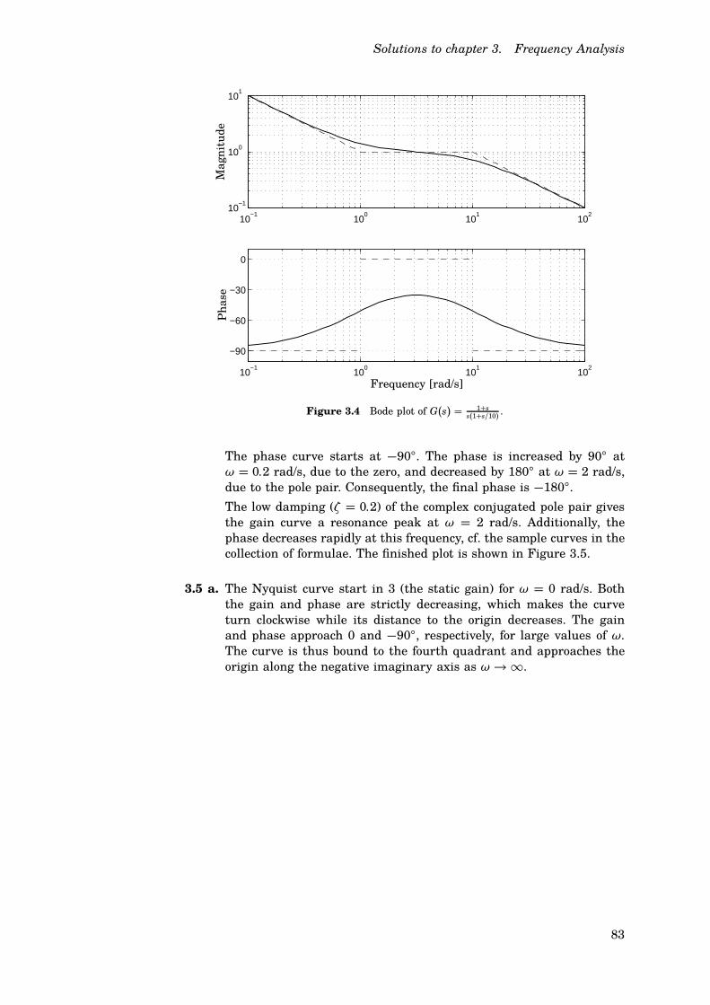
Solutions to chapter 3. Frequency Analysis
10−1
100
101
102
10−1
100
101
10−1
100
101
102
−90
−60
−30
0
Magn
itu
de
Ph
ase
Frequency [rad/s]
Figure 3.4 Bode plot of G(s) = 1+ss(1+s/10) .
The phase curve starts at −90○. The phase is increased by 90○ atω = 0.2 rad/s, due to the zero, and decreased by 180○ at ω = 2 rad/s,due to the pole pair. Consequently, the final phase is −180○.
The low damping (ζ = 0.2) of the complex conjugated pole pair givesthe gain curve a resonance peak at ω = 2 rad/s. Additionally, thephase decreases rapidly at this frequency, cf. the sample curves in thecollection of formulae. The finished plot is shown in Figure 3.5.
3.5 a. The Nyquist curve start in 3 (the static gain) for ω = 0 rad/s. Boththe gain and phase are strictly decreasing, which makes the curveturn clockwise while its distance to the origin decreases. The gainand phase approach 0 and −90○, respectively, for large values of ω.The curve is thus bound to the fourth quadrant and approaches theorigin along the negative imaginary axis as ω →∞.
83

Solutions to chapter 3. Frequency Analysis
10−2
10−1
100
101
100
101
102
10−2
10−1
100
101
−180
−135
−90
−45
0
Magn
itu
de
Ph
ase
Frequency [rad/s]
Figure 3.5 Bode plot of G(s) = 2(1+5s)s(1+0.2s+0.25s2) .
Aided by this analysis, one can now sketch the Nyquist curve bychoosing a few frequencies (e.g. ω = 1, 10 and 100 rad/s) and drawingthe corresponding points in the complex plane. The finished curve isshown in Figure 3.6.
−0.5 0 0.5 1 1.5 2 2.5 3 3.5
−2
−1.5
−1
−0.5
0
0.5
Im
Re
Figure 3.6 Nyquist curve of G(s) = 31+s/10 .
b. The Nyquist curve starts in 10 (the static gain) for ω = 0 rad/s.Both the gain and phase are strictly decreasing, which makes thecurve turn clockwise while its distance to the origin decreases. Thegain and phase approach 0 and −180○, respectively, for large valuesof ω. The curve will thus go from the fourth to the third quadrant,approaching the origin along the negative real axis as ω →∞.
84

Solutions to chapter 3. Frequency Analysis
The intersection with the negative imaginary axis can be drawn byreading off the magnitude when the phase is −90○. One can nowsketch the Nyquist curve by choosing a few additional frequencies(e.g. ω = 0.1, 1 rad/s) and drawing the corresponding points in thecomplex plane. The finished curve is shown in Figure 3.7.
−2 0 2 4 6 8 10 12
−6
−4
−2
0
2
Im
Re
Figure 3.7 Nyquist curve of G(s) = 10(1+10s)(1+s) .
c. The Nyquist curve starts in 1 (the static gain) for ω = 0 rad/s. Boththe gain and phase are strictly decreasing, which makes the curveturn clockwise while its distance to the origin decreases. The gainand phase approach 0 and −∞, respectively, for large values of ω.The curve will thus rotate infinitely many times as it approaches theorigin. The first intersections with the axis can be drawn by readingoff the magnitude when the phase is −90○, −180○, −270○ and −360○,respectively. The finished curve is shown in Figure 3.8.
−1 −0.5 0 0.5 1 1.5
−1
−0.5
0
0.5
Im
Re
Figure 3.8 Nyquist curve of G(s) = e−s
1+s.
85

Solutions to chapter 3. Frequency Analysis
3.6 Let the sought transfer function be G(s). The gain curve starts withslope −1, which indicates that G(s) contains a factor 1
s (an integrator).We observe that there are two corner frequencies: ω1 = 1 and ω2 =100 rad/s. The gain curve breaks upwards once at ω1 and downwardonce at ω2. Hence, the nominator hosts a factor 1 + s, whereas thedenominator contains a factor 1+ s/100. In addition, G(s) contains aconstant gain K . We thus have
G(s) = K(1+ s)s(1+ s/100)
We evaluate the low frequency asymptote of the gain curve at e.g.ω = 0.01 rad/s, in order to determine K . This yields
pG(0.01i)p = K0.01 = 1 [ K = 0.01
Finally we verify that the phase curve matches this system.
3.7 Let the sought transfer function be G(s). The gain curve has twocorner frequencies: ω1 = 2 and ω2 = 100 rad/s. The gain curve breaksdownwards once at ω1 and three times at ω2. Thus the denominatorof G(s) contains the factors (1+ s
2) and (1+ s100)
3. The slope of the lowfrequency asymptote is 1. Thus G(s) has a factor s in the nominator.Additionally, G(s) contains a constant gain K . We have
G(s) = Ks
(1+ s2)(1+ s
100 )3
The factor K is computed by determining a point on the LF asymptote,e.g. GLF(s) = Ks
pGLF(iω)p = Kω = 1
for ω = 0.5 rad/s. This gives
K = 2
Finally we verify by checking that the phase curve matches this sys-tem.
86

Solutions to Chapter 4. Feedback Systems
4.1 a. Laplace transformation of the differential equation yields
sY (s) + 0.01Y (s) = 0.01U(s)
The transfer function GP(s) is thus given by
Y (s) = GP(s)U(s) =0.01
s+ 0.01U(s)
b. The transfer function of the closed loop system becomes
G(s) = GP(s)GR(s)1+ GP(s)GR(s)
=0.01
s+0.01 K
1+ 0.01s+0.01 K
= 0.01K
s+ 0.01+ 0.01K
c. The desired and actual characteristic polynomials are the same if alltheir coefficients match. Identification of coefficients yields
0.1 = 0.01+ 0.01K \ K = 9
4.2 Since r(t) = 0, the control error becomes e(t) = −y(t).
Y (s) = GP(s)(F(s) −GR(s)Y (s)) \ Y (s) = GP(s)1+ GR(s)GP(s)
F(s)
If f (t) is a unit step, we have F(s) = 1s.
a. Seek y(∞) for GR = K
y(∞) = lims→0
sY (s) = lims→0
s1
(ms2 + ds+ K)1
s= 1
K
The function sY (s) has all poles in the left-half plane when the pa-rameters m, d and K are positive.
b. The same assignment, but with GR(s) = K1 + K2/s. This yields
y(∞) = lims→0
s1
(ms2 + ds+ K1 + K2s )
1
s
= lims→0
s
ms3 + ds2 + K1s+ K2= 0
under the assumption of stability, which is the case for m > 0, d > 0and K1 > m
d K2 > 0. Rule: If the disturbance is a step, one needs at
least one integrator before the point in the block diagram where thedisturbance is introduced, in order to make the stationary error zero.
87

Solutions to chapter 4. Feedback Systems
4.3 a. For the closed loop system it holds, when R = 0, that
U(s) = K(0− Y (s)) = −K(GP(s)U(s) + N(s))
from which one obtains
U(s) = −K
1+ KGP(s)N(s)
Y (s) = GP(s)U(s) + N(s) = 1
1+ KGP(s)N(s)
(4.1)
b. Inserting GP(s) = 1s+1 into (4.1) yields the relations
U(s) = −K(s+ 1)s+ 1+ K
N(s)
Y (s) = GP(s)U(s) + N(s) = s+ 1
s+ 1+ KN(s) =: Gyn(s)N(s)
In stationarity it holds that
y(t) = ApGyn(iω)p sin(ωt+ arg Gyn(iω))
= A
√1+ω2
√
(K + 1)2 +ω2sin
(
ωt+ arctanω − arctanω
K + 1
)
u(t) = −Ky(t)
= −K A
√1+ω2
√
(K + 1)2 +ω2sin
(
ωt+ arctanω − arctanω
K + 1
)
c. With A = 1 and K = 1 the amplitudes of the oscillations in u and y
become
Au =
√
1+ω2
4+ω2
Ay =
√
1+ω2
4+ω2
For ω = 0.1 rad/s the amplitudes become
Au ( 0.5
Ay ( 0.5
while ω = 10 rad/s yieldsAu ( 1
Ay ( 1
4.4 With GP(s) = 1/(Js2) we obtain
E(s) = θref (s) − θ(s)= θref (s) −GP(s)(M(s) + KGR(s)E(s))
[ E(s) = 1
1+ KGP(s)GR(s)θref (s) −
GP(s)1+ KGP(s)GR(s)
M(s)
88

Solutions to chapter 4. Feedback Systems
Assume step changes in disturbance momentum M0d and reference
θ 0ref . We postulate GR(s) = Q(s)/P(S), which gives
E(s) = 1
1+ KQ(s)
Js2 P(s)
·θ 0
ref
s−
1
Js2
1+ KQ(s)
Js2 P(s)
·M0
d
s
= s2J P(s)s2J P(s) + KQ(s) ·
θ 0ref
s− P(s)
s2J P(s) + KQ(s) ·M0
d
s
The stationary error becomes
e∞ = limt→∞
e(t) = lims→0
sE(s)
= 0− P(0)KQ(0)M0
d = −P(0)
KQ(0)M0d
where we have assumed that Q(0) ,= 0 and that the conditions for thefinal value theorem are fulfilled. We see that P(0) = 0 yields e∞ = 0.In order to eliminate persistent angular errors caused by disturbancemomenta, it is consequently required to utilize a controller GR(s) withat least one pole in the origin (P(0) = 0).
4.5 The input of the thermocouple is the temperature u(t) of the bath,which gives
u(t) = t [ U(s) = 1
s2
The output y(t) is the reading of the temperature sensor. Thus
Y (s) = G(s)U(s) = 1
1+ sT·
1
s2
For the error e(t) = u(t) − y(t) it holds that
E(s) = U(s) − Y (s) = 1
s2
[
1− 1
1+ sT
]
= sT
1+ sT·
1
s2
The stationary error is obtained by means of the final value theorem
e(∞) = lims→0
sE(s) = lims→0
s2T
1+ sT
1
s2= T = 10
The thermocouple measurement is hence 10○ less than the actualtemperature. I.e. the actual temperature of the bath is 102.6○C +10○C = 112.6○C.
Observe that the error in this has a bounded limit, despite the factthat both u(t) and y(t) lack (bounded) limits as t → ∞. It is thedifference between u and y which converges to a constant value.
89

Solutions to chapter 4. Feedback Systems
4.6 The low frequency asymptote is
GLF(s) =K
s2
where the constant K is given by
pGLF(iω)p =K
ω2; pGLF(i)p = 1 [ K = 1
At the corner frequency ω1 = 1 rad/s the slope changes from −2 to 0,and at ω2 = 5 rad/s it changes from 0 to −1. The transfer function forthe open loop system is thus
Go(s) =(1+ sT1)2s2(1+ sT2)
where T1 = 1/ω1 = 1 and T2 = 1/ω2 = 0.2.
The transfer function of the closed loop system becomes
G(s) = Go(s)1+Go(s)
The output is Y (s) = G(s)R(s) and the error E(s) becomes
E(s) = R(s) − Y (s) = 1
1+ GoR(s) = s2(1+ 0.2s)
s2(1+ 0.2s) + (1+ s)2 R(s)
a.
R(s) = a
s[ e∞ = lim
t→∞e(t) = lim
s→0sE(s)
= lims→0
as2(1+ 0.2s)s2(1+ 0.2s) + (1+ s)2 = 0
The system can thus track inputs r(t) = a without a stationary error.
b.
R(s) = b
s2[ e∞ = lim
t→∞e(t) = lim
s→0sE(s)
= lims→0
bs(1 + 0.2s)s2(1+ 0.2s) + (1+ s)2 = 0
−
The system can also track inputs r(t) = bt without a stationary error.
c.
R(s) = 2c
s3[ e∞ = lim
t→∞e(t) = lim
s→0sE(s)
= lims→0
2c(1+ 0.2s)s2(1+ 0.2s) + (1+ s)2 = 2c ,= 0
The input r(t) = ct2, however, yields a stationary error.
d. Superposition can be used, since the closed loop system is linear andtime invariant (LTI). Here, the input is the sum of the inputs in sub-assignments a and b. The total (superpositioned) stationary error thusbecomes e∞ = 0+ 0 = 0.
90

Solutions to chapter 4. Feedback Systems
e. The input r(t) = sin(t) yields
R(s) = 1
1+ s2[ lim
s→0sE(s)
= lims→0
ss2(1+ 0.2s)
(s2(1+ 0.2s) + (1+ s)2)(1+ s2) = 0
but the input r(t) = sin(t) yields the output y(t) = yo sin(t+φ), where
yo = pG(i)p , φ = ar� G(i)
once transients have decayed. The error e(t) = r(t) − y(t) is thus alsoa sinusoid and the limit
limt→∞
e(t)
does not exist. This shows that the final value theorem should not beused without caution. It is only valid for cases where a limit reallyexists. The criterion is that all poles of sE(s) must have negative realparts. (The factor s2 + 1 in the denominator yields two poles on theimaginary axis.)
4.7 a. The sensitivity function is given by
S(s) = 1
1+ GP(s)GR(s)= 1
1+ 6.5(s+1)3
= s3 + 3s2 + 3s+ 1
s3 + 3s2 + 3s+ 7.5
b. For ω = 0 rad/s we have pS(iω)p = 1/7.5. Low-frequency load distur-bances are thus damped by a factor 7.5.
c. The sensitivity functions has its maximum value pS(iω)p =( 10 atω ( 1.6 rad/s.
4.8 a. The left curve shows the complementary sensitivity function, whereasthe sensitivity function is given by the right curve.
b. The disturbances at various frequencies are amplified according to thegain curve of the sensitivity function. Disturbances below 2 rad/s arehence reduced, disturbances in the range 0.2 to 2 rad/s are amplifiedand disturbances above 2 rad/s pass straight through. The worst casegain, 2, is obtained at the frequency 0.55 rad/s.
c. The complementary sensitivity function, corresponding to the closedloop transfer function from r to y, lies close to 1 up to approximately0.7 rad/s.
d. The maximal magnitude of the sensitivity function equals the inverseof the minimal distance between the Nyquist curve and the point −1.The minimal distance is thus 1/2 = 0.5. The distance to −1, as theNyqist curve intersects the negative real axis, must hence be at least0.5. This implies that the gain margin is at least 2.
91

Solutions to chapter 4. Feedback Systems
4.9 The closed loop transfer function is given by
G(s) = Go
1+ Go= K
s2 + 2s+ K
The poles of the closed loop system are given by the characteristicequation
s2 + 2s+ K = 0 [ s = −1±√
1− K
For K = 0 the roots s1,2 = 0,−2, i.e. the poles of the open loop system,are obtained. The closed loop system G(s) has a double pole in s = −1for K = 1. And as K →∞ the roots become
s1,2 = −1± i∞
The root locus, i.e. the roots of the characteristic equation as K varies,is shown in Figure 4.1 .
Figure 4.1 Root locus of the system in assignment 4.9.
4.10 The open loop transfer function of the system is
Go(s) =K(s+ 10)(s+ 11)
s(s + 1)(s + 2) = KQ(s)P(s)
The closed loop system becomes
G(s) = Go(s)1+ Go(s)
= KQ(s)P(s) + KQ(s)
92

Solutions to chapter 4. Feedback Systems
The characteristic equation is thus
P(s) + KQ(s) = 0
\s(s+ 1)(s+ 2) + K(s+ 10)(s+ 11) = 0
\s3 + (3+ K)s2 + (2+ 21K)s+ 110K = 0
a. The criterion for stability is that all coefficients of the characteristicpolynomial
s3 + (3+ K)s2 + (2+ 21K)s+ 110K
are positive and that
(3+ K)(2+ 21K) > 110K
The inequality yields
K2 − 15
7K + 2
7> 0
It is fulfilled for K > 2 and K < 1/7. The closed loop system is hencestable for
0 < K < 1
7
andK > 2
b. Find the root locus for the characteristic equation, P(s) + KQ(s) = 0
s(s+ 1)(s + 2) + K(s+ 10)(s + 11) = 0 (4.2)
Let n = the degree of P(s) and m = the degree of Q(s). The root locushas a maximum of max(n, m) = 3 branches.
Starting points:
P(s) = 0 [ s = 0,−1,−2
Ending points:Q(s) = 0 [ s = −10,−11
The third branch will approach infinity.
To the right of each real point of the root locus, there must exists anodd number of zeros of P(s) and Q(s). The points x, which fulfill thisare
x < −11 − 10 < x < −2 − 1 < x < 0
The root locus has pn − mp = 1 asymptote. This is the negative realaxis, since the range x < −11 on the real axis belongs to the rootlocus.
The intersection with the imaginary axis is obtained by introducings = iω (4) above. This yields
−(3+ K)ω2 + 110K + i(−ω3 + (2+ 21K)ω) = 0
93

Solutions to chapter 4. Feedback Systems
The resulting equation has a solution ω = K = 0 and
{
−(3+ K)ω2 + 110K = 0
ω2 − (2+ 21K) = 0
gives K = 1/7, ω = ±√
5 or K = 2, ω = ±√
44.
We know from sub-assignment a that the closed loop system is unsta-ble for 1/7 < K < 2. Consequently, the root locus lies in the right halfplane for these values of K . The principal shape of the root locus isshown in Figure 4.2.
Figure 4.2 Root locus of the system in assignment 4.10.
4.11a. The open loop transfer function of the system is
G0(s) =K
s(s + 1)(s + 2)
The closed loop transfer function is thus
Gcl(s) =G0(s)
1+ G0(s)= K
s(s+ 1)(s+ 2) + K
The system is asymptotically stable if all zeros of the characteristicpolynomial
s(s+ 1)(s+ 2) + K = s3 + 3s2 + 2s+ K
have negative real parts. This is the case if all coefficients are positiveand if
3 · 2 > K
The system is thus asymptotically stable if 0 < K < 6.
94

Solutions to chapter 4. Feedback Systems
b. Now we want to study the dependence of K on the stationary error,as the reference increases as a linear function of time. The Laplacetransform of the control error is given by
E(s) = 1
1+ G0R(s) = s(s+ 1)(s+ 2)
s(s+ 1)(s+ 2) + KR(s)
With r(t) = 0.1t, i.e. R(s) = 0.1/s2, we obtain
E(s) = 0.1(s+ 1)(s + 2)s(s(s + 1)(s+ 2) + K)
The signal sE(s) has all poles in the left-half plane when 0 < K < 6,according to sub-assignment a. For this case we can utilize the finalvalue theorem
e(∞) = lims→0
s0.1(s+ 1)(s + 2)
s(s(s + 1)(s+ 2) + K) =0.2
K
In order to obtain a stationary error less than 5 mV for the givenreference, it is required that K > 40. For such large values of K
the system is, however, not stable. It it hence impossible to meet thespecification.
4.12 According to the Nyquist theorem, the closed loop system is stableexactly for those K > 0, which are also
a. K < 2
b. K < 1/1.5 = 2/3
c. K < 1/1.5 = 2/3
d. K < 1/(2/3) = 1.5
4.13 The Nyquist curve intersects the negative real axis when arg(G0(iω)) =−π , i.e. when
−3 arctan(ω) = −π
This is fulfilled whenω = tan
π
3=√
3
The intersection point is given by
pG0(i√
3)p = 1
8
This means that the system is stable for K < 8.
4.14 The system is stable for
0 < K < 1
3.5\ 0 < K < 0.29
as well as
1 < K < 1
0.5\ 1 < K < 2
95

Solutions to chapter 4. Feedback Systems
4.15 The easiest way to solve the problem is through the Nyquist theorem.The transfer function of the process is
GP(s) =e−9s
(1+ 20s)2
The phase shift of the process is
arg GP(iω) = −9ω − 2 arctan(20ω)
We seek the frequency for which the phase shift is−180○. It is obtainedby solving the equation
−9ω − 2 arctan(20ω) = −π
The equation lacks an analytic solution. However, it can be solvednumerically in several ways. The solution is
ω0 ( 0.1
The next step is to determine the process gain for the given frequency.
pG(iω0)p =1
1+ 400ω20
= 0.2
This gives us the gain margin
Am =1
0.2= 5
The gain K = 5 is thus the maximal admissible gain.
4.16 The loop transfer function is
GP(s)GR(s) = e−sL·
10(1+ 12s)
(1+ 10s) = e−sL·
5(1+ 2s)s(1+ 10s)
The cross-over frequency is the frequency where the magnitude of theloop transfer function is equal to one.
pG0(iω c)p =5√
1+ 4ω2c
ω c
√
1+ 100ω2c
= 1
The equation can be solved numerically or analytically
25(1+ 4ω2c) = ω2
c(1+ 100ω2c)
ω4c − 0.99ω2
c − 0.25 = 0
ω2c ( 1.199
ω c ( 1.1 rad/min
The phase at this frequency is
arg G0(iω c) = arctan 2ω c − arctan 10ω c − 90○ −ω c L
96

Solutions to chapter 4. Feedback Systems
The requirement of the phase margin, φm ≥ 10○, gives
φm = 180○ + arg G0(iω c)= 180○ + arctan 2ω c − arctan 10ω c − 90○ −ω c L
( 70○ −ω c L ≥ 10○
This gives the following limit for the time delay L:
L ≤ 60
ω c·
π
180= 1 min
The time delay must therefore be less than one minute.
4.17a. True. Am = 1/pKGP(iω0)p, where ω0 is the frequency for which theNyquist curve intersects the negative real axis.
b. True. φm =π + arg GP(iω) for pGP(iω)p = 1.
c. False. As K is decreased, all points on the Nyquist curve move closerto the origin. Thus the phase margin increases as K is decreased.
d. True. The system is stable for K = 1 and all poles of GP(s) lie inthe left half plane. Consequently, the simplified Nyquist criterion canbe applied. For K = 2, the point −1 lies to the right of the Nyquistcurve, when it is traversed as ω increases. The closed loop system isthus stable.
4.18a. This is the definition of the gain margin. From the plot one sees thatthe phase −180○ corresponds to the gain ∼ 0.4. This yields the gainmargin 1/0.4 = 2.5.
b. This is the definition of the phase margin. From the plot one seesthat for gain 1, the phase is approximately −140○. This yields a phasemargin of approximately 180○ − 140○ = 40○.
4.19 The cross-over frequency and phase margin are read to be ω c = 0.07and φm = 40○, respectively. The delay margin becomes
Lm =φm
ω c= 40○ · π
180○
0.07= 10
97

Solutions to Chapter 5. State Feedback and
Kalman Filtering
5.1 a. From the controllability matrix
Ws =
B AB
=
β 1− β
1 −2
we obtain det Ws = −β − 1, i.e. controllability for all β ,= −1.
b. The observability matrix
Wo =
C
C A
=
0 γ
0 −2γ
has zero determinant independent of γ , i.e. the system is not observ-able for any value of γ .
5.2 The controllability matrix is given by
Ws =
B AB
=
4 −8
−2 4
The controllable states are determined by the columns of Ws and aregiven as α(2,−1)T , where α is a scalar.
5.3
Wo =
C
C A
=
1 1
−1 −1
We see that Wo is singular (det Wo = 0). The state x is non-observableif and only if (iff)
Wox = 0
We obtain a non-observable x iff x1 + x2 = 0. The non-observablestates are thus given by
x = α
1
−1
where α is a number ,= 0.
5.4 The controllability matrix
Ws =
B AB
=
1 −1
0 0
is singular, yielding an uncontrollable system. We can, however, con-duct a more detailed investigation. The system can be written
dx1
dt= −x1 + u, x1(0) = 1
dx2
dt= −2x2, x2(0) = 1
98

Solutions to chapter 5. State Feedback and Kalman Filtering
Hence x2(t) = x2(0)e−2t = e−2t, independent of the applied controlsignal u. On the contrary, x1 can be controlled by means of u, to takeon any desired value. Thus, x2 → 0 as t →∞. The states (x1, x2)whichcan be reached in finite time t < ∞ make up the band 0 < x2 < 1 inFigure 5.1.
x
x
1
2
1
Figure 5.1 Reachable states in assignment 5.4.
As a consequence, only the states
3
0.5
and
10
0.1
can be reached
in finite time.
5.5 The system is controllable, since
Ws =
B AB
=
1 4
2 −7
has full rank.
5.6 a.
Ws =
B AB
=
5 −10
0 0
Ws has rank 1, i.e. the system is not controllable. The states whichcan be reached in finite time from the origin are determined by thecolumns of Ws. The controllable states can be parametrized by t asx = t · (1 0)T .
b. G(s) = C(sI − A)−1B+ D = 5/(s+ 2).
c. The following is a minimal state space representation of G(s){
x = −2x+ 5u
y = x
5.7 a. True. Since the system is controllable, one can place the poles of theclosed loop system arbitrarily by means of linear feedback from allstate variables.
99

Solutions to chapter 5. State Feedback and Kalman Filtering
b. False. A linear state feedback does not affect the zeros of the closedloop system.
c. True if the system is observable.
d. True if the system is observable.
5.8 The closed loop system becomes
{
x = (A− BL)x + Blrr
y = Cx
The characteristic equation is thus
det(sI − A+ BL) = s2 + (3+ l1 + 2l2)s+ 2(1+ l1 + l2) = 0
We need (s+ 4)2 = s2 + 8s + 16 = 0. Identification of coefficientsyields l1 = 9, l2 = −2. The closed loop transfer function is G(s) =C(sI − A+ BL)−1Blr. The stationary gain is G(0) is unity if
G(0) = C(−A+ BL)−1Blr =
lr
4= 1
yielding lr = 4.
5.9 a. The characteristic polynomial of the closed loop system is given by
det(sI − (A− BL)) =∣∣∣∣
s+ 0.5+ 3l1 3l2
−1 s
∣∣∣∣ = s2 + (0.5+ 3l1)s+ 3l2
The desired characteristic polynomial is
(s+ 4+ 4i)(s+ 4− 4i) = s2 + 8s+ 32
Identification of coefficients yields
L =
5/2 32/3
=
2.5 10.7
The closed loop system transfer function is Gyr(s) = C(sI − A +BL)−1Blr. The stationary gain is unity if
Gyr(0) = C(−A+ BL)−1Blr =3
32lr = 1
which yields lr = 32/3.
b. According to a rule of thumb, the observer poles shall be chosen 1.5–2times faster than the state feedback. Place the poles of the Kalmanfilter so that the distance from the origin is twice as large, leading tothe following characteristic polynomial
(s+ 8+ 8i)(s+ 8− 8i) = s2 + 16s+ 128
100

Solutions to chapter 5. State Feedback and Kalman Filtering
The characteristic polynomial of the Kalman filter is given by
det(sI−(A− KC)) =∣∣∣∣
s+ 0.5 k1
−1 s+ k2
∣∣∣∣ = s2+(0.5+ k2)s+0.5k2+ k1
Identification of coefficients yields
K =
120.25
15.5
5.10a. From the block diagram we see that
X1 =1
sK1U
X2 = K21
sX1
X3 =1
sX2
which gives
x1 = K1u
x2 = K2x1
x3 = x2
y = x3
In matrix form we get
x =
0 0 0
K2 0 0
0 1 0
x+
K1
0
0
u
y =
0 0 1
x
b. The feedback law is given by
u = lrr− Lx
The closed-loop system becomes
x = Ax+ B(lrr− Lx) = (A− BL)x + Blrr
The poles of the closed-loop system are given by the eigenvalues ofA− BL, i.e., the roots of the closed loop characteristic equation
det(sI − (A− BL)) = det
s+ K1l1 K1l2 K1l3
−K2 s 0
0 −1 s
= s3 + K1l1s2 + K1 K2l2s+ K1 K2l3 = 0
101

Solutions to chapter 5. State Feedback and Kalman Filtering
The poles of the closed loop system are given by the eigenvalues ofA− BL, i.e. the roots of the closed loop characteristic equation
(s+ 0.5)3 = s3 + 1.5s2 + 0.75s+ 0.125 = 0
One immediately obtains the solution
l1 =1.5
K1
l2 =0.75
K1 K2
l3 =0.125
K1 K2
5.11 The augmented system becomes
d
dt
x1
x2
x3
=
A 0
−C 0
x1
x2
x3
+
B
0
u+
0
1
r
=
0 1 0
0 0 0
−1 0 0
︸ ︷︷ ︸
Ae
x1
x2
x3
︸ ︷︷ ︸
xe
+
0
1
0
︸ ︷︷ ︸
Be
u+
0
0
1
︸ ︷︷ ︸
Br
r
We seek Le =
l1 l2 l3
such that
det(sI − (Ae − Be Le)) = (s+α)(s2 + 2ζωs +ω2)
Insertion of Ae, Be and Le into the above expression yields
s3 + l2s2 + l1s− l3 " s3 + (α + 2ζω)s2 + (ω2 + 2ζωα)s +αω2
Identifications of coefficients now yields
l1 = ω2 + 2ζωα
l2 = α + 2ζω
l3 = −αω2
5.12 The estimation error x fulfills ˙x = (A−KC)x. where K =
k1 k2
T
.
The characteristic equation of the estimation error becomes
det(sI − (A− KC)) = s2 + (4+ k2)s+ k1 + 2k2 + 3 = 0
The desired characteristic equation is
(s+ 4)2 = s2 + 8s+ 16 = 0
Identification of coefficients yields k1 = 5, k2 = 4.
102

Solutions to chapter 5. State Feedback and Kalman Filtering
5.13a. The characteristic equation of the closed loop system is given by
det(
sI−(A− BL))
=∣∣∣∣
s+ 4+ l1 3+ l2
−1 s
∣∣∣∣ = s2+(4+ l1)s+ 3+ l2 = 0
The desired characteristic equation is
(s+ 4)2 = s2 + 8s+ 16 = 0
Which yields l1 = 4 and l2 = 13. The control law becomes
u = −l1x1 − l2x2 = −4x1 − 13x2
b. The states shall be estimated by means of a Kalman filter, i.e.
dx
dt= Ax+ Bu + K(y− Cx)
For x we havedx
dt= (A− KC)x
Determine K such that all eigenvalues of the matrix A − KC areplaced in λ = −6.
det(λI − A+ KC) = λ2 + (4+ k1 + 3k2)λ+ 3+ 3k1 + 9k2
= (λ+ 6)2 = λ2 + 12λ+ 36
Identify the coefficients and solve for k1 and k2:
{
4+ k1 + 3k2 = 12
3+ 3k1 + 9k2 = 36[
{
k1 + 3k2 = 8
k1 + 3k2 = 11
The system of equations lacks solution, see the comment below.
c. The states are to be estimated by a Kalman filter, for which theeigenvalues of A− KC shall be chosen such that
λ2 + (4+ k1 + 3k2)λ+ 3+ 3k1 + 9k2 = (λ+ 3)2 = λ2 + 6λ+ 9
Identifying coefficients and solving for k1 and k2 yields
{
4+ k1 + 3k2 = 6
3+ 3k1 + 9k2 = 9[
{
k1 + 3k2 = 2
k1 + 3k2 = 2
This leaves only one equation, which implies that there exists infinitelymany solutions, e.g. k1 = 2, k2 = 0 or k1 = 0, k2 = 2
3 etc.
The drawback of the proposed observer pole placement is that it yieldsan estimation slower than the closed loop system. This does not affect
103

Solutions to chapter 5. State Feedback and Kalman Filtering
the response to reference changes, which is governed by the poles ofthe closed loop system. However, the handling of process disturbancesbecomes slower.
Comment
An inspection of the system’s observability shows that
det Wo =∣∣∣∣∣
C
C A
∣∣∣∣∣=
∣∣∣∣∣
1 3
−1 −3
∣∣∣∣∣= 0
I.e. the system is not observable. The transfer function of the systemis given by
G(s) = C(sI − A)−1B = s+ 3
s2 + 4s+ 3= 1
s+ 1
The eigenvalue −3 corresponds to a non-observable mode. The modeis, however, controllable, which follows from the canonical controllableform realization of the system. The characteristic equation of A− KC
can be written
det(λI − A+ KC) = (λ+ 3)(λ+ k1 + 3k2 + 1)
This means that the Kalman filter has to estimate the non-observablemode with its own speed. I.e. (at least) one of the eigenvalues ofA − KC must be placed in −3. This explains the failure to computea Kalman filter when the eigenvalues were to be placed in −6 and asuccess when they were to be placed in −3. Note that in cases such asthis one, the result is either that there does not exist a solution K tothe Kalman filter problem, or that it exists infinitely many solutions.When the system is observable, there exists a unique solution K tothe Kalman filter.
104

Solutions to Chapter 6. Design methods
6.1 a. The frequency function of the controller is given by
GR(iω) = K
(
1+ i(ωTd −1
ωTi))
The gain and phase shift for a frequency ω are directly obtainedfrom the gain function A(ω) and phase function φω of the controller,respectively.
A(ω) = pGR(iω)p = K
√
1+ (ωTd −1
ωTi)2
φ(ω) = arg GR(iω) = arctan(ωTd −1
ωTi)
b. We immediately realize that the gain function A(ω) has a uniqueminimum for Im A(iω) = 0, which means that
ωmin =1√
TiTd
At this frequency the gain and phase shift are given by
A(ωmin) = K
φ(ωmin) = 0
Note that the phase shift is negative for ω < ωmin (phase lag) andpositive for ω > ωmin (phase lead).
6.2 a. The dashed gain curve is identical to the nominal one, except that it israised by a factor 4. This is thus the case where K has been multipliedby 4. Observe that the dashed phase curve is not visible in the plotsince it coincides with the solid phase curve. The dotted gain curvediffers from the nominal (solid) curve at low frequencies, for which it islower. This indicates that Ti has been increased, resulting in decreasedlow frequency gain. Also note that the phase curve has been raised forlow frequencies. The last (dash-dotted) curve apparently correspondsto the case where Td has been increased. This is further indicatedby the factor 4 raise of the gain curve for high frequencies. Also forthis case, one can notice a certain increase in the phase, although forsomewhat higher frequencies.
The dashed step response is faster and less damped than the nominal(solid) one. This is a characteristic sign of an increased gain K . Thecorresponding Bode plot confirmingly shows that the cutoff frequency,ω c, has increased (faster), while the phase margin has decreased (lessdamped. The dotted step response features a slow mode both in thereference- and load disturbance responses. Observe the relatively fastincrease in the reference response to approximately 0.8, followed by aslow convergence to 1. This must be due to decreased integral action.
105

Solutions to chapter 6. Design methods
The integral time Ti has thus increased in this case. The correspondingBode plot shows that ω c is virtually unchanged. This is seen in thestep response by the fact that the first part has approximately thesame speed as the nominal case, whereas the following slow settlingis due to the decreased low frequency gain. The last (dash-dotted)step response obviously corresponds to an increase of the derivativetime Td. The reference response is subject to an fast initial increase,followed by a somewhat slower settling. This is seen in the Bode plotby the fact that the high frequency gain has increased, while thelow frequency gain has remained unchanged. The load response issomewhat slower and more damped than in the nominal case.
b. The dashed gain curve is lowered by a factor 2 in comparison to thenominal one, corresponding to a decreased value of K . The dashedphase curve consequently coincides with the nominal (solid) case.The dotted gain curve has been increased for low frequencies, i.e. Ti
has decreased. The dash-dotted gain curve has been lowered at highfrequencies, i.e. Td has decreased.
The dashed step response is slower and more damped than the nomi-nal one. This indicates that K has decreased, since neither a decreasein Ti nor Td would yield a more damped step response. This is furtherconfirmed by the Bode plot. The only case where ω c has decreased iswhen K has decreased. It is also the only case for which the phasemargin has increased. The two remaining step responses are both lessdamped than the nominal one. In order to determine which of thesecorresponds to a decrease of Ti, we look at the corresponding Bode plot(the dotted one). This shows that the cutoff frequency ω c has increasedsomewhat compared to the other nominal case. The dash-dotted Bodeplot, however, shows that the decrease of Td has not changed ω c. Thedotted step response is initially somewhat faster than the nominal(solid) one, whereas the dash-dotted one is initially approximately asfast as the nominal one. This implies that the dotted step responsecorresponds to a decrease in Ti, while the dash-dotted one correspondsto a decrease in Td.
6.3 The transfer function of the process is given by
GP =C
Js+ D
and the transfer function of the PI controller is given by
GR = K
(
1+ 1
sTi
)
We can now write down the closed loop transfer function Gcl as
Gcl =GRGP
1+ GRGP
The characteristic polynomial is the denominator of Gcl
s2 + D + CK
Js+ CK
JTi
106

Solutions to chapter 6. Design methods
and the desired characteristic polynomial is
s2 + 2ζωs +ω2
Identification of coefficients yields
K = 2ζωJ − D
C
Ti =2ζωJ − D
ω2J
6.4 The transfer function of the process, Gp, is given by
Θ = GP I = ki
Js2 + DsI
and the transfer function of the PID controller, GR, is given by
I = GR(Θref − Θ) = K
(
1+ 1
sTi+ sTd
)
(Θref − Θ)
where Θref is the Laplace transform of the reference value of θ . Thetransfer function of the closed loop system, G, is thus given by
Θ = GΘref =GRGP
1+GRGPΘref
The characteristic polynomial is given by the denominator of G and is
s3 + D + K kiTd
Js2 + K ki
Js+ K ki
JTi
We hence arrive at the polynomial equation
(s+α)(s2 + 2ζωs +ω2) = s3 + (α + 2ζω)s2 + (2αζω +ω2)s+αω2
Identification of coefficients yields the equations
D + K kiTd
J= α + 2ζω
K ki
J= 2αζω +ω2
K ki
JTi= αω2
from which one can calculate the sought controller parameters
K = J
ki(2αζω +ω2)
Ti =2ζ
ω+ 1
α
Td =α + 2ζω − D/J
2αζω +ω2
107
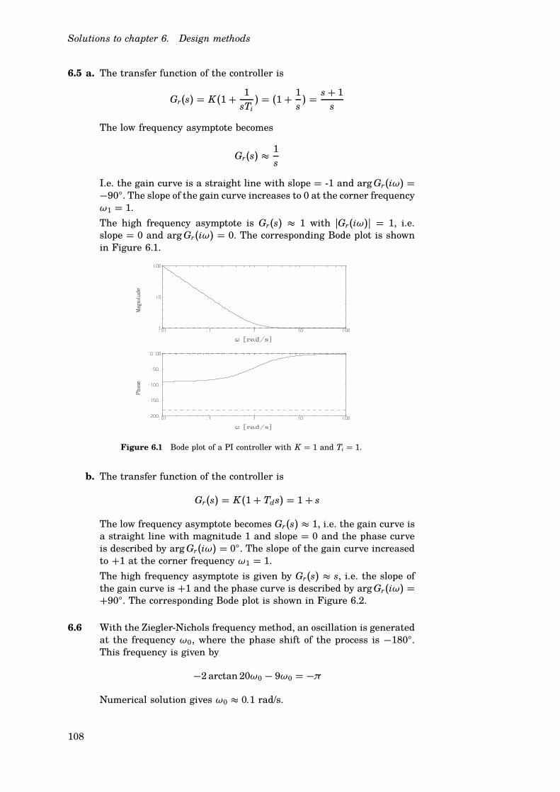
Solutions to chapter 6. Design methods
6.5 a. The transfer function of the controller is
Gr(s) = K(1+ 1
sTi) = (1+ 1
s) = s+ 1
s
The low frequency asymptote becomes
Gr(s) (1
s
I.e. the gain curve is a straight line with slope = -1 and arg Gr(iω) =−90○. The slope of the gain curve increases to 0 at the corner frequencyω1 = 1.
The high frequency asymptote is Gr(s) ( 1 with pGr(iω)p = 1, i.e.slope = 0 and arg Gr(iω) = 0. The corresponding Bode plot is shownin Figure 6.1.
Figure 6.1 Bode plot of a PI controller with K = 1 and Ti = 1.
b. The transfer function of the controller is
Gr(s) = K(1+ Tds) = 1+ s
The low frequency asymptote becomes Gr(s) ( 1, i.e. the gain curve isa straight line with magnitude 1 and slope = 0 and the phase curveis described by arg Gr(iω) = 0○. The slope of the gain curve increasedto +1 at the corner frequency ω1 = 1.
The high frequency asymptote is given by Gr(s) ( s, i.e. the slope ofthe gain curve is +1 and the phase curve is described by arg Gr(iω) =+90○. The corresponding Bode plot is shown in Figure 6.2.
6.6 With the Ziegler-Nichols frequency method, an oscillation is generatedat the frequency ω0, where the phase shift of the process is −180○.This frequency is given by
−2 arctan 20ω0 − 9ω0 = −π
Numerical solution gives ω0 ( 0.1 rad/s.
108

Solutions to chapter 6. Design methods
Figure 6.2 Bode plot of a PD controller with K = 1 and Td = 1.
The process gain at ω0 is
1
1+ 202ω20
= 0.2
The critical gain Kc becomes
Kc =1
0.2= 5
and the period time is
To =2π
ωo= 63
The controller parameters become
{
K = 0.45Kc = 2.25
Ti = To/1.2 = 53
6.7 a. Laplace transform of Martins dynamics give
sX = − 1
30X + 1
15U
Y = X
and the transfer function Y = GPU becomes
GP =2
30s+ 1
The process is controlled by a PI controller, U = GR(R − Y ) where
GR = K(1+ 1
Tis) = K
Tis+ 1
Tis
109

Solutions to chapter 6. Design methods
The controller parameters K and Ti should be chosen such that theclosed loop transfer function Y = Gcl R has its poles in −0.1. Thetransfer function from R to Y is
Gcl =GPGR
1+ GPGR=
K Tis+1Tis
230s+1
1+ K Tis+1Tis
230s+1
= K(Tis+ 1)2Tis(30s + 1) + K(Tis+ 1)2
where the denominator polynomial has the same roots as
s2 + 2K + 1
30s+ K
Ti15
These roots should be −0.1, i.e., the same as for
(s+ 0.1)2 = s2 + 0.2s+ 0.01
This is true if the coefficients for the polynomials are equal, i.e.,
2K + 1
30= 0.2
K
Ti15= 0.01
The controller parameters thus become
K = 2.5
Ti = 16.7
b. When using Ziegler-Nichols frequency method, an experiment is per-formed using feedback with a P controller. The gain is increased untilthe system starts oscillating (stability boundary). The Bode diagramof the process can be thought of as the Bode diagram for the looptransfer function, when the controller is a P controller with a gain of1. When the gain is increased, the gain curve in the Bode diagram willmove upwards, whereas the phase will remain unaffected. The systemwill start to oscillate when the phase margin becomes 0. In the figureit can be seen that this will happen when the cutoff frequency is 0.3rad/s, since the phase curve crosses −180○ at this frequency. This isthe resonant frequency, with which the system will oscillate. For thisfrequency, the gain is equal to 0.2. Thus, a gain of 5 is needed inorder for the system to start oscillating with the resonant frequency.According to the collection of formulae, we have
K = 0.45K0
Ti = T0/1.2
where K0 is the gain and T0 the period time of the oscillation. With
K0 = 5
T0 =2π
0.3= 20.9
we get the controller parameters K = 2.25 and Ti = 17.4.
110

Solutions to chapter 6. Design methods
6.8 Ziegler-Nichols step response method: With the customary notion weobtain a = 0.3 and b = 0.8. The controller parameters become K =1.2/a = 4, Ti = 2b = 1.6 and Td = b/2 = 0.4.
Ziegler-Nichols frequency method: The Nyquist curve intersects thenegative real axis in −1/3 for ω = 1 rad/s, which yields To = 2π/ω =2π and Kc = 3. The controller parameters become K = 0.6Kc = 1.8,Ti = To/2 = 3.1 and Td = To/8 = 0.8.
The Lambda method: By drawing the tangent to the step response,an approximation of the dead time is obtained, L ( 0.8s. The stepresponse has reached 63% of its final value after approximately 2.6s.The time constant thus becomes T = 2.6− 0.8 = 1.8s. The static gainis K P = 1. With λ = T, we get the PI controller parameters
K = 1
Kp
T
L + λ( 0.7
Ti = T = 1.8s
For a PID controller, we get the parameters
K = 1
Kp
L/2+ T
L/2+ λ= 1
Ti = T + L/2 = 2.2s
Td =T L
L + 2T= 0.33s
6.9 a. The step response of the system is shown in Figure 6.3.
Figure 6.3 Step response of G(s) = e−s/(s+ 1).
From the figure we obtain (with the customary notion) a = b = 1.This yields the controller parameters K = 1.2/a = 1.2, Ti = 2b = 2and Td = b/2 = 0.5.
b. The resonance frequency is determined by arg G(iω0) = − arctanω0−ω0 = −π . Numerical solution yields ω0 ( 2.03, resulting in T =2π/ω0 = 3.1.
Further, K0 = 1/pG(iω0)p = 2.26, which gives K = 1.4, Ti = 1.5 andTd = 0.39.
111

Solutions to chapter 6. Design methods
c. From the step response in subproblem a, we get the process parame-ters K P = 1, L = 1 and T = 1. This gives the controller parameters
K = 1
Kp
L/2+ T
L/2+ λ= 1
Ti = T + L/2 = 1.5
Td =T L
L + 2T( 0.33
6.10a. The figure does not allow for any greater precision. Draw the tangentof the step response where the derivative attains a maximum andstudy the intersection of the tangent and the two coordinate axis. Theparameter a is given by the distance between 0 and the intersectionwith the vertical axis, whereas b is given by the distance between 0and the intersection with the horizontal axis. In our example we havea= 0.65 and b = 4. From the table we obtain the following controllerparameters: K = 1.9, Ti = 8 and Td = 2.
b. The critical gain Kc is the gain which causes the Nyquist curve topass through -1. In our case we have Kc = 1/0.55 = 1.8. The criticalperiod T0 corresponds to the frequency at ’o’, i.e. T0 = 2π/ω = 14.6.This yields the controller parameters: K = 1.1, Ti = 7.3 and Td = 1.8.
c. The value of K obtained from the last method is smaller than thevalues obtained through Ziegler-Nichol’s methods.
6.11 Generally it is required that pGK(iω c)p > 1 in order for ω c to increase.
A The speed of the system increases, but simultaneously its robust-ness is reduced since the phase margin decreases.
B pGK p < 1 for all ω, resulting in decreased cross-over frequency andspeed.
C Cf. B.
D pGK p = 1 for all ω, leaving the cross-over frequency unaffected.
6.12 The process is connected in a feedback loop with a proportional con-troller. By adding a compensation link one wants to decrease theramp error of the compensated system by a factor 10. Simultaneously,a small decrease in robustness (phase margin) is accepted, resultingin a certain decrease of the system’s transient behavior.
We can affect the ramp error by introducing a phase lag compensationlink
Gk(s) = Ms+ a
sM + a
Assuming that the system is stable, the resulting ramp error becomes
limt→∞
e(t) = lims→0
sE(s) = lims→0
s ·1
1+ Gk(s)GP(s)·
1
s2
= lims→0
(sM + a)(s+ 1)(s+ 2)s(sM + a)(s+ 1)(s + 2) + K M(s+ a) =
2
K M
112

Solutions to chapter 6. Design methods
By choosing M = 10 (K = 1) the ramp error is reduced to 0.2.
Now it remains to decide a value for a. The phase lag link contributesto a phase lag in the open loop. The phase lag is largest around thefrequency ω = a/
√M . In order not to compound the transient behav-
ior of the closed loop system excessively, a must be chosen such thatthe phase around the cross-over frequency is left unaffected. This canbe achieved by choosing a adequately small. However, a overly smallvalue of a results in a long time before the ramp error decreases to 0.2.Let ω c denote the cross-over frequency of the uncompensated system.At this frequency, the compensation link has a phase contribution
arg Gk(iω c) = arctanω c
a− arctan
Mω c
a
A simple rule of thumb is to choose a = 0.1ω c. In our example itmeans that the compensation link contributes with a phase shift of
arg Gk(iω c) = arctan 10− arctan 100 ( −5.1○
The crossover frequency may be determined numerically according to
pGP(iω c)p =1
ω c
√
1+ω2c
√
4+ω2c
= 1
which gives ω c ( 0.45-
The compensation link thus becomes
Gk(s) = 10s+ 0.045
10s+ 0.045= s+ 0.045
s+ 0.0045
Figure 6.4 Bode plot of the uncompensated open loop system (solid line) and com-pensated open loop system (dash-dotted line) in assignment 6.12. K = 1 for bothcases.
113

Solutions to chapter 6. Design methods
In Figure 6.4 Bode plots for both the uncompensated open loop sys-tem KGP(s) and the compensated open loop system KGk(s)GP(s) areshown.
The compensation link alters the transient behavior of the system.Figure 6.5 shows how the overshoot of the step response has increased,compared to the uncompensated system. Also the settling time hasincreased, partly due to the slow mode in the compensation link.The purpose of introducing the compensation link was to decrease
0 10 20 30 40 50
0
0.5
1
1.5
Figure 6.5 Step responses of the uncompensated closed loop system (solid line) andthe compensated closed loop system (dashed line) in assignment 6.12.
the ramp error. Figure 6.6 shows the error e = r − y for both theuncompensated and compensated systems, with r = t.
As seen from the figure, the compensated system fulfills the criterionof a ramp error less than 0.2.
0 20 40 60 80 100
0
1
2
3
Figure 6.6 Ramp error of the uncompensated system (solid line) as well as thecompensated system (dashed line) in assignment 6.12.
6.13 Use a phase lag compensation link
Gk(s) = K Ns+ b
s+ bN
114

Solutions to chapter 6. Design methods
The crossover frequency ω c of the uncompensated system can be readfrom the Bode plot in Figure 6.7. One can also determine ω c from the
Figure 6.7 Bode plot of the uncompensated open loop system (solid line) as well asthe compensated open loop system (dash-dotted line) in assignment 6.13.
equation
pGP(iω c)p =1.1
ω c
√
ω2c + 1
= 1
This yields ω c = 0.84. The new cross-over frequency is chosen tobe ω∗
c = 1.68. The phase shift of the uncompensated system at thefrequency ω c is
arg GP(iω c) = −90o − arctan(0.84) = −130o
In order not to decrease the phase margin, it must hold that
arg(Gk(iω∗
c )GP(iω∗
c )) ≥ arg GP(iω c)
We have
arg GP(iω∗
c ) = −90o − arctan(1.68) = −149o
For the compensation link it must hence hold that
arg Gk(iω∗
c ) ≥ 19o
From the collection of formulae we find that N = 2 is adequate. Thecompensation link has its maximal phase shift at the frequency b
√N.
This shall occur at the new cross-over frequency, i.e.
ω∗
c = b√
N [ b = ω∗c√N= 1.2
115

Solutions to chapter 6. Design methods
Now choose K such that ω∗c becomes the actual cross-over frequency
(observe that pGk(iω∗c )p = K
√N)
pGk(iω∗
c )GP(iω∗
c )p = 1 [ K = 2.1
We thus obtain the compensation link
Gk(s) = 4.2s+ 1.2
s+ 2.4
Figure 6.7 shows the Bode plot of the uncompensated open loop sys-tem GP(s) as well as the compensated open loop system Gk(s)GP(s).Figure 6.8 shows the step responses of the uncompensated and com-pensated systems.
0 5 10 15 20
0
0.5
1
1.5
Figure 6.8 Step response of the uncompensated closed loop system (solid line) aswell as the compensated closed loop system (dashed line) in assignment 6.13.
6.14 We choose a phase lead link
Gk(s) = K K · Ns+ b
s + bN
The specification implies that the low frequency gain shall not de-crease (which would increase the stationary error). The cross-overfrequency shall increase by a factor 3 and the phase margin shallremain unchanged.
The open loop transfer function is
G0(s) = Gk(s)G1(s) = K K · Ns+ b
s + bN·
1
s(s + 1)(s + 2)
The Bode plot of G1 is presented in Figure 6.9. From this, or fromnumerical calculations, the cross-over frequency is determined to ω c =0.45 rad/s and the phase margin is φm = 53○. The new cross-overfrequency shall thus be ω∗
c = 3 · ω c = 1.35 rad/s with unchangedphase margin. Since arg G1(iω∗
c ) ( −180○, the phase curve must beraised approximately 50○ by Gk.
116

Solutions to chapter 6. Design methods
Figure 6.9 Bode plot of the uncompensated system G1 (solid line) and compensatedsystem GkG1 (dash-dotted line) in assignment 6.14.
From the collection of formulae it is obtained that N = 8 gives amaximal phase lead of approximately 50○. The phase lead is maximalat the frequency b
√N = ω∗
c , yielding b = 0.48. The gain shall beunity at the new cross-over frequency ω∗
c , i.e.
pGk(iω∗
c )p · pG1(iω∗
c )p = 1
The magnitude of the compensator is pGk(iω∗c )p = K K
√N. Numerical
calculations give pG1(iω∗c )p = 0.183. Hence
K K =1√
N · 0.183= 1.9
The step response of the uncompensated and compensated systems,respectively, are shown in Figure 6.10 and the ramp response is shownin Figure 6.11. Since K K > 1 the stationary errors become smallerthan before, thus fulfilling the specifications.
6.15 From the Bode plot of Go(s) (see Figure 6.12) we obtain φm = 20○
and ω c = 0.7 rad/s. Unchanged speed necessitates a compensationlink which does not affect the cross-over frequency. We hence need aphase lead of ∆φ = 30○ at ω = ω c = 0.7 rad/s. We utilize a phase leadcompensation link
Gk(s) = K Ns+ b
s+ bN
1. The sample curves in the collection of formulae yield N = 3.
2. b√
N = ω c [ b = 0.7√3= 0.40
3. pGk(iω c)Go(iω c)p = K√
N · 1 gives K = 1√N= 0.58
117

Solutions to chapter 6. Design methods
0 5 10 15 20
0
0.5
1
1.5
Figure 6.10 The step response of the uncompensated closed loop system (solid line)as well as the compensated closed loop system (dashed line) in assignment 6.14.
0 2 4 6 8 10
0
2
4
6
8
10
Figure 6.11 The ramp response of the uncompensated system (solid line) as wellas the compensated system (dashed line) in assignment 6.14.
The compensation link thus becomes
Gk(s) = 0.58 · 3s+ 0.4
s+ 1.2
The system is stable, so the resulting stationary error becomes
E(s) = 1
1+ GkGoR(s) = s(s+ 0.5)(s+ 3)(s+ bN)
s(s+ 0.5)(s+ 3)(s+ bN) + 2K N(s+ b) R(s)
With R(s) = 1/s2 the stationary ramp error becomes
lims→0
sE(s) = 1.5
2K= 1.29
which fulfills the specification. Figure 6.13 shows the step responseof the system before and after the compensation. The ramp error isshown in Figure 6.14. The fact that the ramp error is increased by thecompensation is due to K < 1.
118

Solutions to chapter 6. Design methods
Figure 6.12 Bode plot of Go(s) in assignment 6.15.
0 10 20 30
0
0.5
1
1.5
2 y(t)
Figure 6.13 Step response of the uncompensated closed loop system (solid line) andcompensated system (dashed line) in assignment 6.15.
6.16 We know that a phase lag compensation link dimensioned according tothe rules of thumb will decrease the phase margin by approximately6○, which yields a certain decrease of robustness. In order not to obtainan excessive overshoot, we start by decreasing the gain of the processin order to increase the phase margin.
From the Bode plot of the process (see Figure 6.15) we find that G− 1has a phase shift of −133○ at the cross-over frequency ω c = 0.7. Atthe frequency ω∗
c = 0.6 we have the phase shift −133○ + 6○ = −127○
and the gain pG1(ω∗c )p = 1.2.
By decreasing the open loop gain by a factor 1.2 we obtain the newcross-over frequency ω∗
c and a phase margin increase of 6○. Sincewe cannot affect the process gain directly, we equivalently let K =
119

Solutions to chapter 6. Design methods
0 10 20 30
0
0.5
1
1.5
2 ramp error e(t)
Figure 6.14 Ramp error of the uncompensated closed loop system (solid line) aswell as the compensated closed loop system (dashed line) in assignment 6.15.
Figure 6.15 Bode plot of the uncompensated open loop system (solid line) as wellas the compensated open loop system (dash-dotted line) in assignment 6.16.
1/1.2 = 0.83 in the compensation link.
The main problem is to decrease the stationary ramp error to e1 ≤ 0.1.The final value theorem gives
e(∞) = lims→0
sU(s) 1
1 +Gk(s)G1(s)=
= lims→0
s1
s2
(s+ a/M)s(s2 + 2s+ 2)(s+ a/M)s(s2 + 2s+ 2) + 1.5K(s+ a) =
2
1.5K M≤ 0.1
which yields M ≥ 16. Choose M = 16. According to the rule of thumbwe let a = 0.1ω∗
c = 0.06. The chosen compensation link thus becomes
Gk(s) = 0.83s+ 0.06
s+ 0.00375
120

Solutions to chapter 6. Design methods
Figure 6.16 shows the step response before and after the compensa-tion. The ramp errors of the uncompensated closed loop system and
0 10 20 30
0
0.5
1
1.5
Figure 6.16 Step response of the uncompensated closed loop system (solid line) aswell as the compensated closed loop system (dashed line) in assignment 6.16.
the compensated closed loop system are shown in Figure 6.17.
0 20 40 60 80
0
1
2
3
Figure 6.17 Ramp error of the uncompensated closed loop system (solid line) aswell as the compensated closed loop system (dashed line) in assignment 6.16.
Comment:
Since we have decreased the open loop gain we obtain a decreasedcross-over frequency and hence a somewhat slower system. In Fig-ure 6.16 one especially notes the slow mode which appears as theprocess settles. It is caused by the slow pole of the controller in com-bination with the low gain. The rise time and damping are, however,virtually unaffected. An alternative to decreasing the open loop gain,in order to maintain the desired phase margin, would be to introducea phase lead compensation link.
121

Solutions to Chapter 7. Controller
Structures
7.1 The disturbance d does obviously lack influence if
G1(s)H(s) + 1 = 0 \ H(s) = − 1
G1(s)
To be a practically useful control law it is required that the distur-bance can be measured, that the model G1(s) of the heating systemis a "good" description of reality and that the inverse transfer func-tion 1/G1(s) is practically realizable. This means that H(s) must notcontain derivatives of the signal d. The realization of H(s) can alsobe problematic if G1(s) lacks a stable inverse (i.e. if G1(s) has righthalf plane zeros, which is equivalent to being a non-minimum phasesystem). Further, we cannot invert processes with low pass character-istics more than at low frequencies and delays can obviously not beinverted.
7.2 A block diagram for the system is shown in Figure 7.1. Mass balance
Σ ΣK ΣG G
G
V T
F
−1
−1
h
v
href x
feedforward
P controller valve tank
Figure 7.1 Block diagram of the level controlling system in assignment 7.2.
for the tank yields
Adh
dt= x(t) − v(t)
Laplace transformation gives ( A = 1 m2)
H(s) = 1
s(X(s) − V(s))
The transfer function of the tank is thus
GT(s) =1
s
a. The closed loop transfer function becomes
G(s) = GTGV K
1+ GTGV K= K
0.5s2 + s+ K
122

Solutions to chapter 7. Controller Structures
The characteristic polynomial is hence
s2 + 2s+ 2K
The desired characteristic polynomial is
(s+ω)2 = s2 + 2ωs+ω2
Identification of coefficients yields
ω = 1
K = 1
2
The transfer function form v(t) to h(t) is given by
H(s) = − GT
1+ GTGV KV(s) = − 1+ 0.5s
s(1+ 0.5s) + KV(s)
If v(t) is a step of amplitude 0.1 we obtain V(s) = 0.1/s. The finalvalue theorem gives
h(∞) = lims→0
sH(s) = −0.1
K
The theorem may be used since sH(s) is of second order with positivecoefficients in the denominator.
b. A PI controller has the transfer function
GR(s) = K(1+ 1
sTi)
The closed loop transfer function becomes
G(s) = GTGV GR
1+ GTGV GR= K(1+ sTi)
s(1+ 0.5s)sTi + K(1+ sTi)
The characteristic polynomial becomes
s3 + 2s2 + 2Ks+ 2K
Ti
The desired characteristic polynomial is
(s+ω)3 = s3 + 3ωs2 + 3ω2s+ω3
Identification of coefficients yields
ω = 2
3
K = 2
3
Ti =9
2
123

Solutions to chapter 7. Controller Structures
c. The relation between the flow disturbance v and the level h is givenby
H(s) = GT(GV GF − 1)1+ GTGV GR
V(s)
To eliminate the influence of v, we choose
GF(s) =1
GV= 1+ 0.5s
Note that GF is not realizable. One can either cancel the derivativeterm or add a low-pass filter so that the infinite gain at high frequen-cies is avoided.
7.3 The closed loop system has the transfer function
(GR + K f )GP
1+GPGR= (K + K f )s+ K/Ti
s2 + (3+ K)s+ K/Ti
a. The characteristic equation of the closed loop system is
s2 + (3+ K)s+ K/Ti = 0
The desired characteristic equation is
(s+ 2− 2i)(s+ 2+ 2i) = s2 + 4s+ 8 = 0
Identification of coefficients yields K = 1 and Ti = 1/8.
b. The feedforward K f affects the zeros of the closed loop system, butleaves the poles unaffected. The poles can be placed by means of thecontroller H in order to obtain adequate supression of disturbances,cf. sub-assignment a above. One can subsequently translate the zerosby means of K f in order to e.g. reach a desired overshoot in the refer-ence step responses. The zero of the closed loop system is eliminatedby choosing K f = −K . With the pole placement in sub-assignment a,which corresponds to a relative damping ζ = 1/
√2 ( 0.7, the over-
shoot of the closed loop system becomes approximately 5%.
7.4 The block diagram in assignment 7.3 can be re-drawn according toFigure 7.2. By comparing to the block diagram in assignment 7.3 wesee that H f f = H + K f and H f b = H. Observe that manipulation ofK f offers the possibility to neutralize the derivation in H, i.e. achievea controller which derivates the output, but not the reference value.
7.5 The system has three inputs: the reference yr and the two disturbancesv1 and v2. The transfer functions between these three signals and theoutput y are given by
Y = G1G2GR1GR2
1+ G1GR1 + G1G2GR1GR2Yr +
G1G2
1+ G1GR1 + G1G2GR1GR2V1
+ (1+ G1GR1)G2
1+ G1GR1 +G1G2GR1GR2V2
124

Solutions to chapter 7. Controller Structures
+ + H G(s)
–1 H
Y r
K f
Figure 7.2 Modified block diagram in assignment 7.3.
Let us call the three transfer functions Gyr, Gv1 and Gv2, respectively.Ideally we would have Gyr = 1 and Gv1 = Gv2 = 0 for all frequencies.This is, however, not achievable. Nonetheless, we can assure thatit holds in stationarity, i.e. for s = 0. For a P controller we haveGR(0) = K , where K is the gain of the controller. For a PI controllerit holds that GR(0) = ∞.
The transfer function Gyr becomes unity if GR2 is a PI controller. Thetransfer function Gv1 becomes 0 if any of the controllers are PI. Thetransfer function Gv2, however, is only zero if GR2 is a PI controller.
Consequently GR2 must contain an integral part in order to guarantee0 stationary control error. The controller GR1 can then be chosen tobe a P controller. (If we furthermore want the internal signal y1 tocoincide with its reference, also this controller would need an integralpart.)
7.6 a. The closed loop transfer function is given by
Ginner(s) =K1G1(s)
1+ K1G1(s)= 2K1
s+ 2+ 2K1
In order to make the system 5 times as fast, the pole of the closedloop system must be placed in s = −10, calling for K1 = 4.
b. The approximation Ginner(s) ( Ginner(0) = 0.8 yields
Gouter(s) =GR2(s)G2(s)Ginner(0)
1+ GR2(s)G2(s)Ginner(0)=
(K2s+ K2Ti)0.8
s2 + 0.8K2s+ 0.8 K2Ti
The specification of a system 10 times slower than the inner loop callsfor a pole in s = −1. Since we deal with a second order system, wechoose to locate both poles in s = −1 (somewhat slower than the singlepole case). This yields K2 = 2.5 and Ti = 2.
125

Solutions to chapter 7. Controller Structures
Comment. A general rule when cascading controllers is to make the innerloop 5–10 times faster than the outer loop in order to enable separation ofthe controller calculations for the two loops. The actual closed loop system(without approximations) becomes
Gouter(s) =10(2s+ 1)
s3 + 10s2 + 20s+ 10
and has poles in approximately −7.516, −1.702 and −0.7815 where theslower pole (s = −0.7815) will be the one essentially determining the speed
of the system. This corresponds fairly well to the specified speed.
7.7 a. Since the steam flow is assumed to be constant, we can let F = 0,which yields the following description of the dome
Y (s) = 10−3
sM(s)
Since the controller is of P type we have M(s) = K(Yr− Y ), where Yr
denotes the reference dome level. This yields
Y (s) = K
K + 103sYr(s)
Since the system is linear and subject to negative feedback, a stepdisturbance in the level gives rise to the same transient behavioras a step disturbance in the reference. Hence let Yr(s) = 1
s . Inversetransformation of Y (s) yields
y(t) = 1− e−K10−3t
The specification on the settling time of the system now yields
y(10) = 1− e−K10−2 = 0.9 [ K = 230
b. The dome and P controller are described by
Y (s) = K
K + 1000sYr(s) +
s− 0.01
(s+ 0.1)(1000s+ K) F(s)
Let Yr(s) = 0. A step disturbance in the steam flow F(s) = 1s thus
gives
Y (s) = s− 0.01
(s+ 0.1)(1000s+ K)1
s
The final value theorem yields
limt→∞
y(t) = lims→0
sY (s) = lims→0
ss− 0.01
(s+ 0.1)(1000s+ K)1
s= −0.1
K
and stationary error becomes
e = yr − y = −y = 0.1
K
126

Solutions to chapter 7. Controller Structures
c. Determine a feedforward link H(s) from steam flow F(s) to feed waterflow M(s) for the initial system, such that the level Y (s) becomesindependent of changes in the steam flow.
The system with feedforward H(s)F(s) is described by
Y (s) = 10−3
s(M(s) + H(s)F(s)) + s− 0.01
s(s+ 0.1)10−3 F(s)
= 10−3
sM(s) + 10−3
s
(
s− 0.01
s+ 0.01+ H(s)
)
F(s)
We want the influence from F(s) to be zero. Therefore choose H(s)so that the expression in front of F(s) becomes zero. This criterion isfulfilled when
H(s) = −s− 0.01
s+ 0.1
which gives the desired feedforward.
7.8 The delay margin is given by
Lm =φm
ω c
First we compute the cross-over frequency ω c as
pG0(iω c)p = pGP(iω c)GR(iω c)p =∣∣∣∣
2
iω c(iω c + 1)
∣∣∣∣ =
2
ω c
√
ω2c + 1
" 1
\ ω4c +ω2
c − 4 = 0 \ ω c =
√
−1+√
17
2= 1.25
Then we calculate the the phase margin φm
φm =π + arg G0(iω c) =π − π
2− arctanω c = 0.675
We thus obtain Lm = φm/ω c = 0.54.
7.9 a. The one second delay e−s is considered part of the process.
Controller GR(s) = K
Process GP(s) =1
s(s + 1) e−s
Model GP(s) = GP(s) =1
s(s + 1) e−s
Model without delay G0P(s) =
1
s(s + 1)
b. According to the block diagram the control signal is given by
U(s) = GR(s)(
E(s) + GP(s)U(s) − G0P(s)U(s)
)
127

Solutions to chapter 7. Controller Structures
10−2
10−1
100
101
102
10−1
100
101
10−2
10−1
100
101
102
−10
0
10
20
30
40
50
60
Magn
itu
de
Ph
ase
Frequency [rad/s]
Figure 7.3 Bode plot of the Smith predictor.
The transfer function of the controller becomes
U(s) = GR(s)1−GR(s)GP(s) + GR(s)G0
P(s)E(s)
= 2
1− 2
s(s + 1) e−s + 2
s(s+ 1)
E(s) = 2s(s+ 1)s(s+ 1) + 2− 2e−s
E(s)
The Bode plot of the controller is shown in Figure 7.3. One notesthat the Smith predictor gives a large phase lead at the cross-overfrequency of the initial system.
c.
U(s) = 2s(s+ 1)s(s+ 1) + 2− 2e−s
E(s) ( 2s(s+ 1)s(s+ 1) + 2− 2(1− s) E(s)
= 2(s+ 1)s+ 3
E(s)
This is a phase lead link with N = 3.
7.10 The gain curve of the system is given by
pG(iω)p = k
ω
It is sufficient to read the value of the gain curve at a single frequencyin order to determine k. The gain is e.g. 1 at approximately ω = 4.5.This yields
1 = k
4.5\ k = 4.5
128

Solutions to chapter 7. Controller Structures
The phase curve of the system is given by
arg G(iω) = −π/2−ω L
Now, it is sufficient to read the value of the phase curve at a single fre-quency in order to determine L. The phase is e.g. −π at approximatelyω = 120. This yields
−π = −π/2− 120L \ L = 0.013
129

Solutions to Chapter 8. Design Examples
8.1 a. The phase curve for v = 3 knots cuts −180○ at ωo ( 0.03 rad/s. At thisfrequency we have pG(i0.03)p ( 2. The gain K must hence be smallerthan 0.5 in order to yield a stable closed loop system.
b. In order to acquire the cross-over frequency ω c and phase margin φm
it is required that
{
pGr(iω c)G(iω c)p = 1
arg Gr(iω c)G(iω c) = φm − 180○
where Gr(s) = K(1+ TDs). This leads to the equations
K pG(iω c)p√
1+ T2Dω2
c = 1
arg G(iω c) + arctan TDω c = φm − 180○
With ω c = 0.03 rad/s, φm = 60○, pG(iω c)p ( 2 and arg G(iω c) ( −180○
we obtain
Td =tan 60○
0.03=√
3
0.03( 57.7
K = 1
pG(iω c)p√
1+ T2dω2
c
( 1
2 · 2= 0.25
c. If the speed suddenly increases from 3 to 7 knots, we have to turnto the dotted Bode plots in Figure 8.2. The most drastic change isthat the gain curve has been raised by a factor 20. Additionally,the phase curve has decreased for frequencies above 0.03 rad/s. Thisresults in heavily reduced phase- and gain margins. A more thoroughexamination shows that this in fact leads to instability of the closedloop system. This can be seen in the Bode plot in Figure 8.2, whichshows both the nominal case v = 3 knots and the case v = 7 knots.
One way to avoid this problem is to instead choose v = 7 knots as thenominal case for the calculation of the PD controller. This, however,means that one has to accept a slower settling time for the slowestspeed v = 3 knots. A better way is to let K and Td depend on thespeed v. This method is known as gain scheduling.
d. The transfer function from β to h can be approximated by
Ghβ (s) =kvv
s3
From the Bode plot one sees that pGhβ (i · 0.1)p ( 0.04 for v = 3 knots= 3 · 1.852/3.6 ( 0.5144 · 3 m/s, which yields
kv (0.13
· 0.04
3 · 0.5144( 2.6 · 10−5
130

Solutions to chapter 8. Design Examples
10−3
10−2
10−1
100
101
102
10−3 10−2 10−1 100
-200
-150
-100
-50
0
10−3 10−2 10−1 100
10−3
10−2
10−1
100
101
102
10−3 10−2 10−1 100
−200
−150
−100
−50
0
10−3 10−2 10−1 100
10−3
10−2
10−1
100
101
102
10−3 10−2 10−1 100
−200
−150
−100
−50
0
10−3 10−2 10−1 100
Magn
itud
eP
hase
[deg]
Frequency [rad/s]
Figure 8.1 Bode plot of the PD compensated open loop system in assignment 8.1.The solid curves show the case v = 7 knots. Note that the latter case yields anunstable closed loop system.
e. The characteristic equation of the closed-loop is given by
s3 + K kvv = 0
Since not all coefficients are positive, the closed-loop system is notasymptotically stable for any value of K . In sub-assignment a it wasconcluded through the measured frequency response that the closedloop system was stable for K < 0.5. The explanation to this ap-parent contradiction is found in the Bode plot which was used insub-assignment a: The approximation only holds for high frequencies(ω > 0.05). For low gains, such as K < 0.5, the cross-over frequencyω c < 0.03 lies outside the valid range of the model.
For e.g. ω < 0.03 the Bode plot shows a phase above −180○ while thesimplified model features the phase −270○ for all frequencies.
f. If x = (α, α, h)T and u = β we obtain the state space equations
x =
0 0 0
1 0 0
0 v 0
x+
kv
0
0
u
With the state feedback u = −Lx + ur the characteristic polynomialof the closed loop system becomes
p(s) = det(sI − A+ BL) = s3 + kvl1s2 + kvl2s+ kvvl3
the desired characteristic polynomial is
p(s) = (s+γω0)(s2+2ζω0s+ω20) = s3+(γ+2ζ )ω0s2+(2γζ+1)ω2
0s+γω30
131

Solutions to chapter 8. Design Examples
Direct comparison gives
l1 =(γ + 2ζ )ω0
kv
l2 =(2γζ + 1)ω2
0
kv
l3 =γω3
0
kvv
g. Here stationarity means constant height, h = href. This in turns meanthat all derivatives of h must be zero, i.e. α = 0 and α = 0. Whenthe height has reached its correct value the control signal u = β mustalso be zero since the submarine would otherwise continue to rise.Thus Lr is obtained from the equation
0 = Lrhref − l1 · 0− l2 · 0− l3href
For v = 3 knots, we end up with the following result
Lr = l3 =γω3
0
kvv( γω3
0·
2.6 · 10−5 · 3 · 0.5144( γω3
0·
4.0 · 10−5
h. At a momentary disturbance ∆h = 0.1 m the rudder angle becomes
∆β = l3 · ∆h = γω30
vkv· 0.1 ( 0.2ω3
0
3 · 0.5144 · 2.6 · 10−5
Since ∆β ≤ 5○, we must have
ω0 ≤(
5 · 3 · 0.5144 · 2.6 · 10−5
0.2
)13
( 0.1
8.2 a. The oscillation frequency ωo ( 27 rad/s and critical gain Kc ( 3.6can be read from the Bode plot. The oscillation period is hence To =2π/ωo ( 0.23. This yields the PID parameters K = 0.6Kc ( 2.2,Ti = To/2 ( 0.12 and Td = To/8 ( 0.03. The step response of theclosed loop system is shown in Figure 8.2. The specifications areapparently not fulfilled. A PID controller (with filter factor) can beconsidered a second order controller with integral action. As a matterof fact, the specifications can be met, using a more general secondorder controller with integral action (see Figure 8.3). If one tries tointerpret it as a PID controller, one would end up with a negativederivative time Td.
b. In stationarity all derivatives of the states must be zero x = 0. Ithence holds that
{
0 = Axo + Buo = (A− BL)xo + BLryr
yr = yo = Cxo
This yields
Lr = −1
C(A− BL)−1B
132

Solutions to chapter 8. Design Examples
0
0.2
0.4
0.6
0.8
1
1.2
1.4
1.6
0 0.1 0.2 0.3 0.4 0.5 0.6 0.7 0.8 0.9 10
0.2
0.4
0.6
0.8
1
1.2
1.4
1.6
0 0.1 0.2 0.3 0.4 0.5 0.6 0.7 0.8 0.9 1
Figure 8.2 The step response with PID control according to Ziegler-Nichols.
0
0.2
0.4
0.6
0.8
1
1.2
1.4
1.6
0 0.1 0.2 0.3 0.4 0.5 0.6 0.7 0.8 0.9 10
0.2
0.4
0.6
0.8
1
1.2
1.4
1.6
0 0.1 0.2 0.3 0.4 0.5 0.6 0.7 0.8 0.9 1
Figure 8.3 The step response of the closed loop system with a second order inte-grating controller.
c. With x augmented to xe = (x1, x2, x3, xi)T we obtain
xe =
− d1+d f
J1
d f
J1− k f
J10
d f
J2− d f+d2
J2
k f
J20
1 −1 0 0
0 kω2 0 0
xe +
km ki
J1
0
0
0
u+
0
0
0
−1
yr
y =
0 kω2 0 0
xe
where the reference yr has been introduces as an extra input.
d. The approximate value of ωm becomes
ωm ( −ln 0.02
0.5 · 0.38( 20
133

Solutions to chapter 8. Design Examples
e. When it comes to load disturbances, the fast Kalman filter (ωo = 40)has the best performance. It is also best when it comes to suppressingthe influence of of measurement noise. However, it is the worst choicewhen it comes to suppressing the influence of noise in the controlsignal. The two cases ωo = 10 and ωo = 20 feature approximatelythe same noise sensitivity, while ωo = 10 is slower when it comes toeliminating load disturbances. A satiable choice is thus ωo = 20.
134

Solutions to Chapter 9. Interactive
Comparison Between Model
Descriptions
9.1
a. The amplitude of the step response is affected, but not the time con-stant. The pole is not affected. The Nyquist diagram keeps its shape,but each point on the curve moves radially from the origin. In theBode diagram, the gain curve changes in the y direction while thephase curve is unchanged.
Since the control signal is a unit step, K is given by the stationaryvalue of the measurement signal in the step response. In the Nyquistdiagram, K is given from the starting point on the positive real axis.In the Bode diagram, K is given from the gain curve where ω → 0.
b. The amplitude of the step response is not affected, but the time con-stant is given by T. The pole is in s = −1/T, which means that a largetime constant gives a pole close to the origin, whereas a short timeconstant gives a pole far away from the origin. In the Bode diagram,the corner frequencty is 1/T, and it thereby varies when T varies.No change is visible in the Nyquist diagram, but the frequency variesalong the curve.
Suppose that we have two processes with different values of T. Then,we can always find two frequencies such that
G(iω1T1) =K
1+ iω1T1= G(iω2T2) =
K
1+ iω2T2
i.e., all points that are on the first Nyquist curve are also on thesecond one, but at another frequency.
c. A variation in L corresponds to a translational movement of the stepresponse. We can not represent a dead time in a singularity diagram.The gain curve in the Bode diagram is not affected, since pe−iω Lp = 1,but the phase is reduced. For each frequency point in the Nyquist dia-gram, the distance to the origin remains unchanged, but the phase de-creases. Since the phase goes towards −∞ when ω →∞, the Nyquistcurve has the spiral shape.
9.2
a. The changes are the same as in problem 1a.
b. The changes are analogous to the ones in problem 1b. When T1 ≫ T2,the step response is similar to the one in problem 1a, with T ( T1. TheBode and Nyquist diagrams are also similar to the ones in problem1a for low frequencies. Thus, you can in many cases approximate thetransfer function by
G(s) = K
(1+ sT1)(1+ sT2)( K
(1+ sT1)
135

Solutions to chapter 9. Interactive Comparison Between Model Descriptions
c. If the zero is far away from the origin, the representations are notsignificantly affected. If the zero is negative and is close to the origin,there is a large overshoot in the step response. If the zero is positiveand close to the origin, the step response will initially go in the wrongdirection. If the zero is positive it will give a positive contribution tothe phase.
When T3 < 0, e.g., when the zero is in the right half plane, the processis hard to control. You can imagine that it is hard for a controller to actin the right way when a control signal change makes the measurementsignal go in the wrong direction initially. The phenomenon could beunderstood by writing the transfer function in the following way
G(s) = K(1+ sT3)(1+ sT1)(1+ sT2)
= K
(1+ sT1)(1+ sT2)+ sKT3
(1+ sT1)(1+ sT2)
Thus, the transfer function consists of two terms, one that is thetransfer function that we had in problem 2a, and one that is the sametransfer function, but multiplied with sT3. Thus, the second term isproportional to the derivative of the measurement signal we wouldhave obtained if we did not have any zero. If T3 < 0, this term willgive a negative contribution, which explains that the step responseinitially goes in the wrong direction.
9.3
a. The frequency ω affects the speed of the system, but not the shape ofthe step response. Variations in ω moves the poles radially from theorigin. In the Bode diagram, ω does not affect the shape, but only thelocation of the corner frequency. The shape of the Nyquist curve is notaffected, but the frequencies are moved along the curve.
b. The relative damping ζ does not affect the speed of the step response,but the shape. A small value of ζ gives an oscillatory and poorlydamped response. A small value of ζ gives a large resonance peak inthe Bode diagram. In the Nyquist diagram, you get a big increase ofgain and fast phase shift around ω.
136