Automatic classification of sulcal regions of the human brain cortex using pattern recognition

Kirsten J. Behnkea,b, Maryam E. Rettmanna,b, Dzung L. Phamc, Dinggang Shend,

Susan M. Resnickb, Christos Davatzikosd, Jerry L. Prince*e

aDept. of Biomedical Engin., Johns Hopkins Univ., 3400 N. Charles St., Baltimore, MD 21218 bGerontology Research Center, NIA/NIH, 5600 Nathon Shock Dr., Baltimore, MD 21224

cNeuroradiology Div., Johns Hopkins Univ., 600 N. Wolfe St. Baltimore, MD 21287 dSect. of Biomed. Image Analysis, Dept of Radiology, Univ. of Penn., Philadelphia, PA 19104

eDept. of Electrical Engin., Johns Hopkins Univ., 3400 N. Charles St., Baltimore, MD 21218

ABSTRACT Parcellation of the cortex has received a great deal of attention in magnetic resonance (MR) image analysis, but its usefulness has been limited by time-consuming algorithms that require manual labeling. An automatic labeling scheme is necessary to accurately and consistently parcellate a large number of brains. The large variation of cortical folding patterns makes automatic labeling a challenging problem, which cannot be solved by deformable atlas registration alone. In this work, an automated classification scheme that consists of a mix of both atlas driven and data driven methods is proposed to label the sulcal regions, which are defined as the gray matter regions of the cortical surface surrounding each sulcus. The premise for this algorithm is that sulcal regions can be classified according to the pattern of anatomical features (e.g. supramarginal gyrus, cuneus, etc.) associated with each region. Using a nearest-neighbor approach, a sulcal region is classified as being in the same class as the sulcus from a set of training data which has the nearest pattern of anatomical features. Using just one subject as training data, the algorithm correctly labeled 83% of the regions that make up the main sulci of the cortex. Keywords: sulcal labeling, human brain cortex, pattern recognition, deformable models, sulci, atlas

1. INTRODUCTION The surface of the human brain cortex is made up of many convoluted folds separated by spaces known as sulci. The classification of these sulci is an important step in many neuroimaging studies, which seek to analyze morphological changes in regions of interest on the cortex that are typically defined by the primary sulci (cf. 1- 5). A sulcal classification scheme would facilitate a parcellation of the cortex into regions that are both functionally and anatomically important. In this work, we present a method to classify the key sulci with the future goal of parcellation in mind. There are many software programs available that a trained neuroanatomist or technician could use to manually label sulci on the brain. 6- 8 Unfortunately, this task is both difficult and time-consuming, and thus a scheme for automatic labeling is necessary. Past efforts at an automated labeling algorithm have involved warping a prelabeled atlas to a preprocessed image of a test brain (cf. 9- 13), thereby transferring labels from the deformed atlas to the appropriate locations on the test brain. Other more recent efforts have favored supervised algorithms in which sulci are matched with models from a training database based on characteristics such as shape, location, or structure. 14- 18 Our method combines key concepts from both approaches. The challenge facing all of the approaches is the high variability in both shape and structure of sulci from subject to subject. To address this problem, our algorithm begins with a data driven sulcal segmentation that is unique to the subject, followed by a classifier which identifies the segmented sulci based on features extracted using a deformable atlas. In this work, we present an algorithm for automatically classifying sulcal regions of the human cortex. We begin with a definition of sulcal regions and a review of the work we have done previously in segmenting these * Send correspondence to prince@jhu.edu; phone: 1 410 516-5192; fax 1 410 516-5566; http://iacl.ece.jhu.edu

regions. We then describe the classification algorithm and report an evaluation of its performance. Finally, we discuss advantages and disadvantages of our method and propose future improvements.

2. BACKGROUND

We propose a technique that automatically classifies the sulcal regions of the cortex, which we have defined in previous reports as the buried regions of the cortex surrounding the sulcal spaces. 19- 21 An illustration of this definition is shown in the cross-section in Figure 1. We believe that this surface representation of sulci is appropriate because neuroimaging studies are typically concerned with function on, or the variability of, regions on the cortical surface. We note that the standard anatomical labeling scheme assigns gyral labels rather than sulcal labels. The difference between the two approaches is that gyral labels include the gyrus and the surrounding regions ending at a fundus, while sulcal regions include the fundus and surrounding regions ending at the gyrus. Both gyral and sulcal labels include the region between the fundus and the gyrus. We use this overlap as an important feature of our classification algorithm. Before we can identify sulcal regions on the cortical surface, we must first construct an accurate representation of the surface. There are many interfaces that we could use to represent the surface of the cortex. These include the gray matter-white matter interface, the gray matter-cerebrospinal fluid interface, and the surface that lies halfway between these interfaces. Although our sulcal segmentation and classification algorithms could be applied to any of these surfaces, we reconstruct the latter — i.e., the central surface. Starting from magnetic resonance (MR) images acquired by the Baltimore Longitudinal Study of Aging, 22, 23 we use a previously described method, 24 along with several improvements, 25- 27 to reconstruct the central surface of the cortex. The final reconstruction consists of a triangular mesh comprised of approximately 300,000 vertices. Once the cortical surface has been reconstructed, we use a previously reported technique 19- 21 to segment the sulcal regions which will later be classified. We now present an overview of this technique; further details can be found in past reports. We note that this sulcal segmentation algorithm is applied to both hemispheres of the cortex separately so that medial sulcal regions can be segmented as well as lateral sulcal regions. The segmentation of the sulcal regions is based on the result of a watershed algorithm that is applied to a geodesic distance transform on the surface of the cortex. The watershed algorithm yields an over-segmentation in which each sulcal region consists of many small pieces known as catchment basins (CB’s). We then apply a merging algorithm which joins CB’s in meaningful ways to define distinct sulcal regions. The merging algorithm is controlled by two thresholds which we specify. The first is a height threshold which defines the minimum height of ridges that divide sulcal regions. If two CB’s are separated by a ridge that is smaller than the height threshold, then the CB’s are merged to form one sulcal region. This rule of merging is based on the observation that only large ridges such as gyri usually separate individual sulci and segments of interrupted sulci. The second threshold constrains the minimum size of the sulcal regions. If the area of a CB is smaller than the area threshold, then the CB is merged with the largest adjacent CB. This is based on the observation that sulcal regions are typically large in area. After merging, each distinct sulcal region is randomly assigned a region label, which is a unique number greater than zero. Finally, a map of the cortical surface is constructed in which each vertex of the triangular mesh has a numerical label. To be more exact, let V be the set of all vertices, vi, on the cortical mesh. Let r(vi) be the region label of each vertex, vi, such that

==

region sulcal aon is vertex if 1,-..., 0, ,gyrus aon is vertex if 0

(i

ii vN pp

vvr ) , (1)

where N is the number of sulcal regions in the segmentation. The task of this work is to assign a sulcal label (e.g. Left Central Sulcus, Right Sylvian Fissure) to each segmented sulcal region. From here on, we will refer to the unknown

fundus

gyrus gyrussulcal region

Figure 1. Cross-section of the cortex illustrating the region referred to as a sulcal region.

sulcal regions in a segmentation as test sulcal regions. We note that the test sulcal regions were formed from the merging of CB’s. The advantage of this method of segmentation is that by varying the values of the two thresholds we can generate many different degrees of segmentation. Furthermore, we can store each of these segmentations in a graph structure, in which test sulcal regions are formed from merged CB’s at the coarsest scale and from individual CB’s at the finest scale. Examples of a coarse segmentation and a fine segmentation are displayed in Figure 2. We have chosen six values for the height threshold ranging from 0 to 10 (mm) and seven values for the area threshold ranging from 0 to 300 (mm2). This gives us the flexibility of 42 different levels of segmentation. While the coarser levels may be sufficient for classifying certain major sulci such as the central sulcus and the sylvian fissure, the finer levels are necessary for classifying sulci that tend to connect to other sulci. For example, the parieto-occipital sulcus and the calcarine sulcus are typically connected; thus, they must be classified at finer levels in which the sulci are segmented as two separate regions, rather than at coarser levels where the two regions are merged into one and can only be assigned one label. There may be an optimal degree of merging, unique to each sulcus, but that is generally unknown a priori.

3. METHODS In this section, we describe an algorithm that classifies test sulcal regions. For simplicity, we first describe how the test sulcal regions from one level of segmentation can be classified. We later describe how all segmentation levels can be incorporated to improve the overall classification performance. For each test sulcal region, we measure features that distinguish it as a member of a particular sulcal class. We also measure the features of manually labeled sulci to construct training data. Finally, we use a simple nearest-neighbor classifier to assign each test sulcal region to one of 14 classes of sulci based on a comparison between the features of the test sulcal region and the features of each sulcal class in the training data. A flow chart for our entire algorithm is shown in Figure 3. 3.1. The training database The classifier that we have implemented is nonparametric; thus, it has the advantage that it does not require a model or estimate of pattern distributions. Instead, it requires a training set that consists of patterns of features that are measured from manually labeled sulci. In this initial investigation, our training set consists of only one subject, on which 14 chosen sulci were manually labeled using the Interactive Program for Sulcal Labeling (IPSL). 7 IPSL is a user interface that allows the user to manually label sulcal regions by selecting the sulcal label and then clicking on the corresponding sulcal region. The sulci were labeled according to the atlas of sulci written by Ono. 28 In addition, sulci that did not belong to one of the 14 classes were assigned a unique null label. In the future, our method can be extended by explicitly naming each null label and attempting to label a much larger group of sulci. Each labeled sulcus represents a sulcal class in the training set. The classifier assigns unknown sulcal regions to the class from the training set that has the most similar pattern of features.

Figure 2. Coarse sulcal segmentation (left) and fine sulcal segmentation (right).

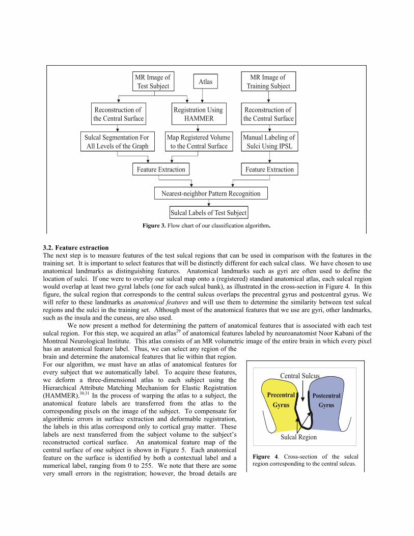
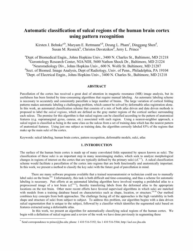
3.2. Feature extraction The next step is to measure features of the test sulcal regions that can be used in comparison with the features in the training set. It is important to select features that will be distinctly different for each sulcal class. We have chosen to use anatomical landmarks as distinguishing features. Anatomical landmarks such as gyri are often used to define the location of sulci. If one were to overlay our sulcal map onto a (registered) standard anatomical atlas, each sulcal region would overlap at least two gyral labels (one for each sulcal bank), as illustrated in the cross-section in Figure 4. In this figure, the sulcal region that corresponds to the central sulcus overlaps the precentral gyrus and postcentral gyrus. We will refer to these landmarks as anatomical features and will use them to determine the similarity between test sulcal regions and the sulci in the training set. Although most of the anatomical features that we use are gyri, other landmarks, such as the insula and the cuneus, are also used. We now present a method for determining the pattern of anatomical features that is associated with each test sulcal region. For this step, we acquired an atlas 29 of anatomical features labeled by neuroanatomist Noor Kabani of the Montreal Neurological Institute. This atlas consists of an MR volumetric image of the entire brain in which every pixel has an anatomical feature label. Thus, we can select any region of the brain and determine the anatomical features that lie within that region. For our algorithm, we must have an atlas of anatomical features for every subject that we automatically label. To acquire these features, we deform a three-dimensional atlas to each subject using the Hierarchical Attribute Matching Mechanism for Elastic Registration (HAMMER). 30, 31 In the process of warping the atlas to a subject, the anatomical feature labels are transferred from the atlas to the corresponding pixels on the image of the subject. To compensate for algorithmic errors in surface extraction and deformable registration, the labels in this atlas correspond only to cortical gray matter. These labels are next transferred from the subject volume to the subject’s reconstructed cortical surface. An anatomical feature map of the central surface of one subject is shown in Figure 5. Each anatomical feature on the surface is identified by both a contextual label and a numerical label, ranging from 0 to 255. We note that there are some very small errors in the registration; however, the broad details are

MR Image of Test Subject

Sulcal Segmentation For All Levels of the Graph

Registration Using HAMMER

Feature Extraction

Sulcal Labels of Test Subject

Nearest-neighbor Pattern Recognition

Manual Labeling of Sulci Using IPSL

Map Registered Volumeto the Central Surface

Reconstruction of the Central Surface

MR Image of Training SubjectAtlas

Reconstruction of the Central Surface

Feature Extraction

Figure 3. Flow chart of our classification algorithm.

Sulcal Region

Central Sulcus

PostcentralGyrus

PrecentralGyrus

Figure 4. Cross-section of the sulcal region corresponding to the central sulcus.

correct and this registration is sufficient for our purpose of extracting anatomical features. When the anatomical features are transferred to the central surface, a map of the central surface is created in which each vertex of the triangular mesh is assigned an anatomical feature label. Again, let V be the set of all vertices, vi, in the map. Let a(vi) be the anatomical feature label of each vertex such that:

0,...,255. b b,)( ==iva (2) Recall from Section 2 that each vertex also has a region label, r(vi). By grouping the vertices with the same region label, we can study one test sulcal region at a time. An anatomical feature associated with a particular test sulcal region can be described quantitatively by the number of vertices within that test sulcal region which are labeled with that anatomical feature. For example, let f be an anatomical feature with the numerical label 5. If we consider test sulcal region 10, then f can be described by the total number of vertices for which r(vi) = 10 and a(vi) = 5. For each test sulcal region, the number associated with each anatomical feature can then be stored in a test feature vector, x = [x1, x2, …, xd]T, where d is the total number of anatomical features in the atlas. Thus, it is the test feature vector that describes the pattern of anatomical features attributed to each test sulcal region. Since each test sulcal region overlaps just a few of the anatomical features, the test feature vectors are very sparse. Similar feature vectors are used to represent the patterns of anatomical features associated with the sulcal classes of the training data. To compile the training set, IPSL was used to manually label the sulcal regions on the reconstructed surface of the brain that was used as the atlas. Since the anatomical features of this brain were pre-labeled, the registration step was unnecessary. The pattern of anatomical feature labels for each known sulcus was determined and stored in a training feature vector, t = [t1, t2, …, td]T. This training feature vector represents the pattern of anatomical features associated with a sulcal class in the training set. Since only one subject was labeled, there is only one training feature vector for each class. 3.3. Subject histograms and training histograms A useful way to compare the similarity between the feature vector of a particular test sulcal region and the training feature vectors is to construct histograms. A subject histogram describes the distribution of features associated with a test sulcal region. The x-axis is the numerical labels of the anatomical features, ak where k=0,…,255; and the y-axis is the number of vertices in the test sulcal region for which a(vi) = k. Likewise, a training histogram describes the distribution of features found in a sulcus of the training set. Examples of subject and training histograms are shown in Figure 6. We note that the anatomical feature labels on the x-axis are indexed by their numerical label. The contextual labels of the prominent anatomical features are added to these figures only for illustrative purposes to make the histograms easier to compare. Furthermore, it is not the exact magnitude of the number of vertices associated with each feature that is important; rather it is the fact that only certain features are prominent. It is clear that the pattern of features in test sulcal region 16 is more similar to the pattern of features associated with sulcal class left superior temporal sulcus.

LeftPostcentralGyrus (#110)

Left PrecentralGyrus (#5)

Figure 5. Anatomical feature labels on the surface of a test subject after registration with the atlas.

3. 4. Nearest-neighbor classification Once the feature vectors are determined, the next step is to design a classifier that will assign the test sulcal region to the class in the training data with the most similar training feature vector. The similarity of the patterns of anatomical features can be described quantitatively by a distance metric. The test sulcal region with feature vector, x, will be classified as the same class as the nearest feature vector, tj, in the training data. The nearest training feature vector is that which minimizes the distance from x to tj. We use the l2 norm as our distance metric. Thus, the nearest training feature vector, tj, is that which satisfies the following equation:

2

11jmin arg j

j

j

t

txx

−= . (3)

Figure 6. Subject histogram (top) displaying the distribution of anatomical features in test sulcal region 16. Training histograms (bottom) displaying the distribution of anatomical features in prelabeled sulci of the training set.

The distance metric in equation 3 is squared to save computation time. The feature vectors in equation 3 are normalized by the 1-norm to account for the fact that test sulcal regions have various sizes and thus vary in total number of vertices.

As a simple classification example, consider an experiment with only three features: precentral gyrus, postcentral gyrus, and superior parietal lobule. In this case, the feature space is 3-dimensional and an example feature space is pictured in Figure 7. The classes are clearly separable and are described by the training feature vectors shown as a triangle, plus sign, and square. They are each normalized so that they lie within the hyper-surface. The normalized feature vector of the test sulcal region to be classified is represented by the star. In this example, the nearest training feature vector is the square. Therefore, the test sulcal region would be classified as belonging to class C. This can be confirmed by substituting the feature vectors into equation 3 and confirming that tC gives the smallest distance.

3.5. Applying the classifier to the graph

In the previous sections, we described a method for classifying the test sulcal regions in any one of the levels of segmentation. However, the graph structure consists of many levels of segmentation. We now present a method for determining which level is optimal for each sulcal class. There are two possibilities. The first is to empirically determine one level of segmentation that is optimal for the majority of the sulci. However, due to the interpersonal variability of sulci, the optimal level of segmentation may be different for each subject. In addition, the chosen level may be optimal for some sulci and very poor for others. The second method proposes a solution to these problems. In this method, all levels of segmentation are incorporated into the classifier. We will now describe this method further. We begin with the task of classifying each of the test regions at the finest level of segmentation. We then track each test sulcal region as it moves up through the levels and is merged with other regions. With each merging, the feature vector of the test sulcal region changes to include the anatomical features of the regions with which it merged. In some cases this causes the test feature vector to move nearer to a training feature vector, while in other cases it will move farther away. After considering all possible mergings, we can determine which training feature vector the test feature vector was nearest to, and assign the sulcal label of that training feature vector to the test sulcal region. In this way, the knowledge at each level of segmentation is incorporated. Furthermore, an optimal level for each sulcus is determined based on the distance metric. Since this optimization is not empirically determined, it is not affected by interpersonal variability.

4. RESULTS We evaluated the accuracy of our classifier by first manually labeling the sulcal regions on ten subjects, and then comparing these labels with labels assigned by the classifier. Using IPSL, we constructed a “truth” sulcal map which

LegendUnknown Feature Vector, x

Class A Feature Vector, tA

Class B Feature Vector, tB

Class C Feature Vector, tC

Precentral Gyrus (#5)

PostcentralGyrus (#110)

Sup. Parietal Lobule (#52)

norm

alize

Figure 7. The feature space for a simple classification example with only three features.

consisted of vertices, vi, of a triangular mesh. The vertices were assigned a truth label, tr(vi), such that

=

=otherwise 0

sulci 14 theof oneon was if 1,...14,z z,( iv

)ivtr . (4)

The sulcal regions were manually labeled according to the same definition as the sulci in the training set. We note that none of the ten test subjects were used in generating the training set.

There are two important types of errors which the classifier may make. The first occurs when a vertex has the truth label, class A, and the classifier assigns it to a class other than A. This is called a miss for class A and the probability that the classifier will miss is called the probability of a false negative. Since we are more interested in how often the classifier detects class A rather than misses, we calculate the probability of detection (Pd). Let Rtr be the region with the truth label, A, and let Rcl be the region labeled A by the classifier. Then the formula for the probability of detection for class A is:

( )

( )trRAreaclRRArea

AdP

tr I= . (5)

The value of Pd can range from 0 to 1. A value of 1 indicates that every vertex which had truth label, A, was correctly labeled class A by the classifier. The other error of interest occurs when the classifier assigns a vertex to class A and that vertex has a truth label which is not equal to A. This is called a false alarm for class A and the probability that the classifier will make false alarms is referred to as the probability of false positives (Pf). The formula for the probability of false positives for class A is:

( ) ( )

( )clRAreaclRRArea- RArea

AfP

trcl I= . (6)

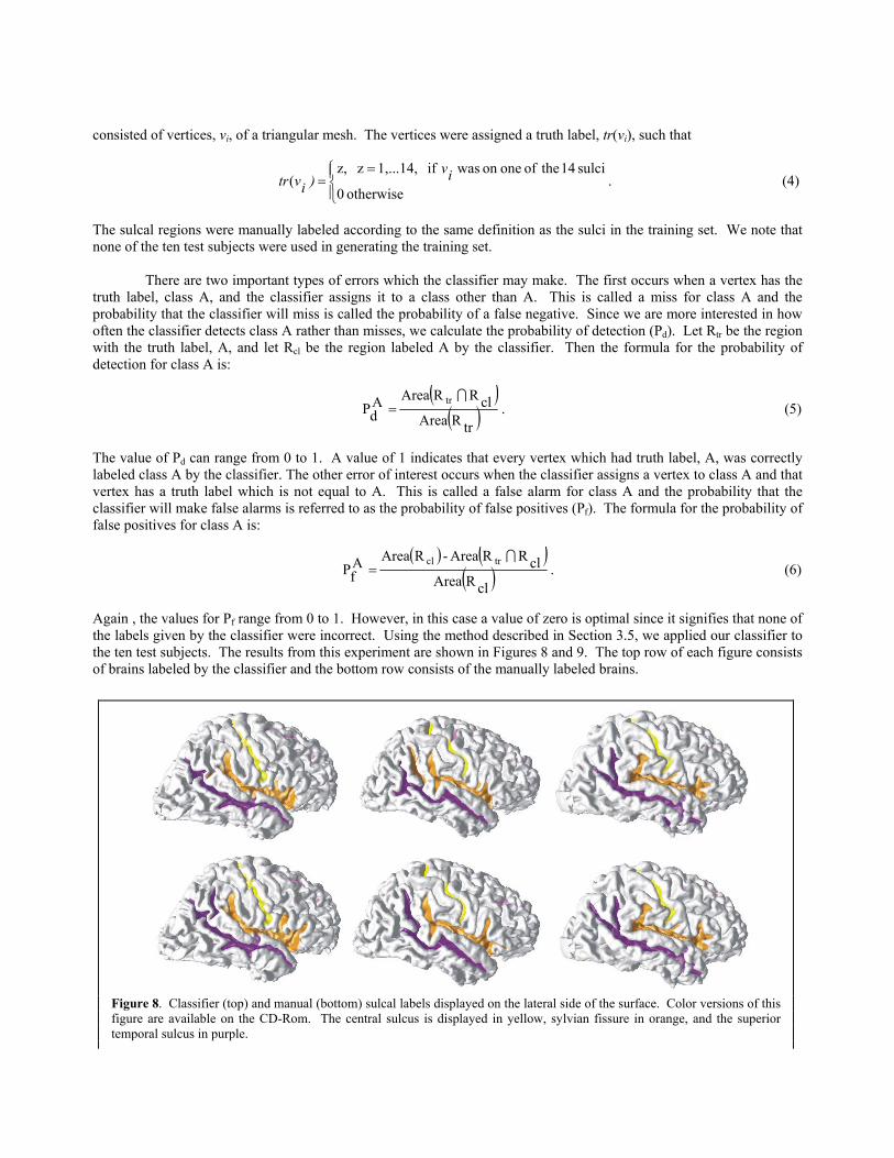
Again , the values for Pf range from 0 to 1. However, in this case a value of zero is optimal since it signifies that none of the labels given by the classifier were incorrect. Using the method described in Section 3.5, we applied our classifier to the ten test subjects. The results from this experiment are shown in Figures 8 and 9. The top row of each figure consists of brains labeled by the classifier and the bottom row consists of the manually labeled brains.

Figure 8. Classifier (top) and manual (bottom) sulcal labels displayed on the lateral side of the surface. Color versions of this figure are available on the CD-Rom. The central sulcus is displayed in yellow, sylvian fissure in orange, and the superior temporal sulcus in purple.

Additionally, the average Pd and Pf for each sulcus in this experiment are displayed in Table 1. To demonstrate that our method of incorporating all levels of segmentation is superior to selecting any one level of segmentation, we applied the classifier to each of the 42 levels separately and these results are displayed in Table 2. The first column displays the Pd that is obtained if the best level is selected for each sulcus. The second column displays the Pd that is obtained if the worst level of segmentation is selected. Finally the third column displays the average Pd.

Table 1. Average probability of detection and average probability of false positives for an experiment with ten subjects.

Sulcal Class Probability of detection Probability of false positives Left Central Sulcus 1.000 0.050 Left Sylvian Fissure 0.828 0.046 Left Superior Temporal Sulcus 0.737 0.185 Left Superior Frontal Sulcus 0.638 0.208 Left Cingulate Sulcus 0.686 0.040 Left Parieto-Occipital Sulcus 0.880 0.226 Left Calcarine Sulcus 0.805 0.159 Right Central Sulcus 1.000 0.058 Right Sylvian Fissure 0.920 0.060 Right Superior Temporal Sulcus 0.836 0.129 Right Superior Frontal Sulcus 0.728 0.297 Right Cingulate Sulcus 0.747 0.021 Right Parieto-Occipital Sulcus 0.987 0.333 Right Calcarine Sulcus 0.720 0.164 Overall sulci 0.835 0.119

Figure 9. Automatic (top) and manual (bottom) sulcal labels displayed on the medial side of the surface. Color versions of this figure are on the CD-Rom. The cingulate sulcus is displayed in blue-violet, calcarine sulcus in maroon, and parieto-occipital sulcus in blue.

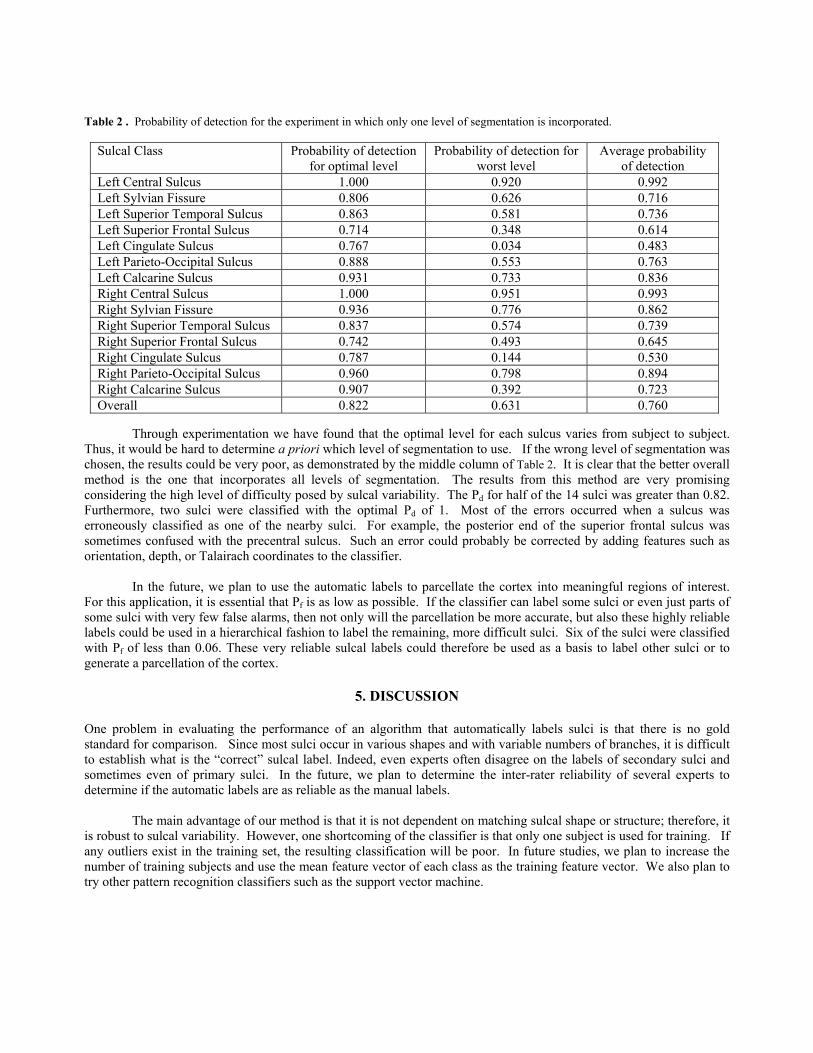
Table 2 . Probability of detection for the experiment in which only one level of segmentation is incorporated.

Sulcal Class Probability of detection for optimal level

Probability of detection for worst level

Average probability of detection

Left Central Sulcus 1.000 0.920 0.992 Left Sylvian Fissure 0.806 0.626 0.716 Left Superior Temporal Sulcus 0.863 0.581 0.736 Left Superior Frontal Sulcus 0.714 0.348 0.614 Left Cingulate Sulcus 0.767 0.034 0.483 Left Parieto-Occipital Sulcus 0.888 0.553 0.763 Left Calcarine Sulcus 0.931 0.733 0.836 Right Central Sulcus 1.000 0.951 0.993 Right Sylvian Fissure 0.936 0.776 0.862 Right Superior Temporal Sulcus 0.837 0.574 0.739 Right Superior Frontal Sulcus 0.742 0.493 0.645 Right Cingulate Sulcus 0.787 0.144 0.530 Right Parieto-Occipital Sulcus 0.960 0.798 0.894 Right Calcarine Sulcus 0.907 0.392 0.723 Overall 0.822 0.631 0.760

Through experimentation we have found that the optimal level for each sulcus varies from subject to subject. Thus, it would be hard to determine a priori which level of segmentation to use. If the wrong level of segmentation was chosen, the results could be very poor, as demonstrated by the middle column of Table 2. It is clear that the better overall method is the one that incorporates all levels of segmentation. The results from this method are very promising considering the high level of difficulty posed by sulcal variability. The Pd for half of the 14 sulci was greater than 0.82. Furthermore, two sulci were classified with the optimal Pd of 1. Most of the errors occurred when a sulcus was erroneously classified as one of the nearby sulci. For example, the posterior end of the superior frontal sulcus was sometimes confused with the precentral sulcus. Such an error could probably be corrected by adding features such as orientation, depth, or Talairach coordinates to the classifier. In the future, we plan to use the automatic labels to parcellate the cortex into meaningful regions of interest. For this application, it is essential that Pf is as low as possible. If the classifier can label some sulci or even just parts of some sulci with very few false alarms, then not only will the parcellation be more accurate, but also these highly reliable labels could be used in a hierarchical fashion to label the remaining, more difficult sulci. Six of the sulci were classified with Pf of less than 0.06. These very reliable sulcal labels could therefore be used as a basis to label other sulci or to generate a parcellation of the cortex.

5. DISCUSSION

One problem in evaluating the performance of an algorithm that automatically labels sulci is that there is no gold standard for comparison. Since most sulci occur in various shapes and with variable numbers of branches, it is difficult to establish what is the “correct” sulcal label. Indeed, even experts often disagree on the labels of secondary sulci and sometimes even of primary sulci. In the future, we plan to determine the inter-rater reliability of several experts to determine if the automatic labels are as reliable as the manual labels. The main advantage of our method is that it is not dependent on matching sulcal shape or structure; therefore, it is robust to sulcal variability. However, one shortcoming of the classifier is that only one subject is used for training. If any outliers exist in the training set, the resulting classification will be poor. In future studies, we plan to increase the number of training subjects and use the mean feature vector of each class as the training feature vector. We also plan to try other pattern recognition classifiers such as the support vector machine.

6. CONCLUSION

In this work, we have presented a method for automatically classifying test sulcal regions on the human brain cortex. The high level of interpersonal variability of sulci was addressed by beginning with a sulcal region segmentation that is unique to the subject and data driven. Our algorithm, which consists of a nearest-neighbor classifier, has shown promising results. In the future, we plan to improve upon it so that it may be used to generate a parcellation of the cortex.

ACKNOWLEDGEMENTS

The authors thank Dr. Noor Kabani for constructing the atlas of anatomical features. The authors also thank Xiao Han for his inspiration in a classification algorithm which incorporates all levels of the graph. This research was supported in part by the NIH/NINDS through grant R01 NS37747.

REFERENCES 1. B. Crespo-Facorro, J. Kim, N. C. Andreasen, D. S. O’Leary, A. K. Wiser, J. M. Bailey, G. Harris, and V. A.

Magnotta, “Human frontal cortex: An MRI-based parcellation method,” NeuroImage. 10(5), pp. 500-519, 1999. 2. J. Kim, B. Crespo-Facorro, N. C. Andreasen, D. S. O’Leary, B. Zhang, G. Harris, and V. A. Magnotta, “An MRI-

based parcellation method for the temporal lobe,” NeuroImage. 11(4), pp. 271-288, 2000. 3. J. Rademacher, V. S. Caviness Jr., H. Steinmetz, A. M. Galaburda, “Topographical variation of the human primary

cortices: implications for neuroimaging, brain mapping, and neurobiology,” Cereb. Cortex. 3, pp. 313-329, 1993. 4. N. Tzourio, L. Petit, E. Mellet, C. Orssaud, F. Crivello, K. Benali, G. Salamon, and B. Mazoyer, “Use of anatomical

parcellation to catalog and study structure-function relationships in the human brain,” Hum. Brain Mapp. 5(4), pp. 228-232, 1997.

5. N. Tzourio-Mazoyer, B. Landeau, D. Papathanassiou, F. Crivello, O. Etard, N. Delcroix, B. Mazoyer and M. Joliot, “Automated anatomical labeling of activations in SPM using a macroscopic anatomical parcellation of the MNI MRI single-subject brain,” NeuroImage. 15(1), pp. 273-289, 2002.

6. D. MacDonald. “Display: a user’s manual,” Tech. Rep., McConnell Brain Imaging Centre, MNI, McGill University, Montreal, 1996.

7. M. E. Rettmann, X. Tao, and J. L. Prince, “Assisted labeling techniques for the human brain cortex,” in Medical Imaging: Image Processing, M. Sonka and J. M. Fitzpatrick, eds., Proc. SPIE 4684, pp. 179-190, 2002.

8. R. Lanzenberger, P. Brugger, D. Prayer, C. Windischberger, A. Geissler, M. Barth, A. Gartus, and R. Beisteiner, “Three dimensional labeling of individual brain sulci,” Hum. Brain Mapp, Poster No. 10485, 2002.

9. S. Jaume, B. Macq, and S. K. Warfield, “Labeling the brain surface using a deformable multiresolution mesh,” in Proc. MICCAI ’02, T. Dohi and R. Kikinis, eds., LNCS 2488, pp. 451-458, 2002.

10. S. Sandor and R. Leahy, “Surface-based labeling of cortical anatomy using a deformable atlas,” IEEE Trans. Med. Imag. 16(1), pp. 41-54, 1997.

11. P. M. Thompson, R. P. Woods, M. S. Mega, and A. W. Toga, “Mathematical/computational challenges in creating deformable and probabilistic atlases of the human brain,” Hum. Brain Mapp. 9, pp. 81-92, 2000.

12. P. M. Thompson, D. MacDonald, M. S. Mega, C. J. Holmes, A. C. Evans, A. W. Toga, “Detection and mapping of abnormal brain structure with a probabilistic atlas of cortical surfaces,” J. of Comput. Assisted Tomogr. 21(4), pp. 576-581, 1997.

13. P. M. Thompson and A. W. Toga. “A surface-based technique for warping three-dimensional images of the brain,” IEEE Trans. Med. Imag. 15(4), pp. 402-417, 1996.

14. A. Caunce and C. J. Taylor, “Using local geometry to build 3D sulcal models,” Proc. IPMI’99, A. Kuba et. al., eds., LNCS 1613, pp. 196-209, 1999.

15. G. Lohmann, D. Y. von Cramon, “Automatic labelling of the human cortical surface using sulcal basins,” Med. Image Analysis. 4, pp. 179-188, 2000.

16. G. Lohmann, D. Y. von Cramon, “Automatic detection and labelling of the human cortical folds in magnetic resonance data sets,” in Computer Vision: ECCV ’98, Vol II, H. Burkhardt, B. Neumann, eds., LNCS 1407, pp. 369-381, 1998.

17. D. Riviere, J. F. Mangin, D. Papadopoulos-Orfanos, J. M. Martinez, V. Frouin, J. Regis, “Automatic recognition of cortical sulci of the human brain using a congregation of neural networks,” Med. Image Analysis 6, pp. 77-92, 2002.

18. G. Le Goualher, E. Procyk, D. L. Collins, R. Venugopal, C. Barillot, and A. C. Evans. “Automated extraction and variability analysis of sulcal neuroanatomy,” IEEE Trans. Med. Imag. 18(3), pp. 206-217, 1999.

19. M. E. Rettmann, X. Han, C. Xu, and J. L. Prince, “Automated sulcal segmentation using watersheds on the cortical surface,” NeuroImage. 15(2), pp. 329-344, 2002.

20. M. E. Rettmann, X. Han, and J. L. Prince, “Watersheds on the cortical surface for automated sulcal segmentation,” in Proc. MMBIA‘00. pp. 20-27, 2000.

21. M. E. Rettmann, C. Xu, D. L. Pham, and J. L. Prince, “Automated segmentation of sulcal regions,” in Proc. MICCAI‘99. C. Taylor and A. C. F. Colchester, eds., Lecture Notes in Computer Science 1679, pp. 158-167, 1999.

22. N. W. Shock, R. C. Greulich, R. Andres, D. Arenburg, P. T. Costa, Jr., E. Lakatta, and J. D. Tobin, “Normal human aging,: The Baltimore Longitudinal Study of Aging,” U.S. Govt. Printing Office, Washington, D.C., 1984.

23. S. M. Resnick, A. F. Goldszal, C. Davatzikos, S. Golski, M. A. Kraut, E. J. Metter, R. N. Bryan, and A. B. Zonderman, “One-year age changes in MRI brain volumes in older adults,” Cereb. Cortex. 10, pp. 464-472, 2000.

24. C. Xu, D. L. Pham, M. E. Rettmann, D. N. Yu, and J. L. Prince, “Reconstruction of the human cerebral cortex from magnetic resonance images,” IEEE Trans. Med. Imag. 18(6), pp. 467-480, 1999.

25. C. Xu, X. Han, and J. L. Prince, “Improving cortical surface reconstruction accuracy using an anatomically consistent gray matter representation,” 6th Int. Conf. on Functional Mapping of the Human Brain. p.S581, 2000.

26. X. Han, C. Xu, M. E. Rettmann, and J. L. Prince, “Automatic segmentation editing for cortical surface reconstruction,” in Medical Imaging 2001: Image Processing, M. Sanka and K. M. Hanson, eds., Proc. SPIE 4322, pp. 194-203, 2001.

27. X. Han, C. Xu, U. Braga-Neto, and J. L. Prince, “Graph-based topology correction for brain cortex segmentation,” in Proc. IPMI’01. pp. 385-391, 2001.

28. M. Ono, S. Kubick, and C. D. Abernathey, Atlas of the Cerebral Sulci, Thieme Med. Pub., Inc., New York, 1990. 29. N. Kabani,D. MacDonald, C. Holmes, A. Evans, “3D atlas of the human brain,” 4th Int. Conf. on Functional

Mapping of the Human Brain, A. Toga, R. Frackowiak, and J. C. Mazziota, eds, NeuroImage 7(4), p. S717, 1998. 30. D. Shen, C. Davatzikos, “HAMMER: hierarchical attribute matching mechanism for elastic registration,” IEEE

Trans. Med. Imag. 21(11), 2002. 31. D. Shen, C. Davatzikos, “HAMMER: hierarchical attribute matching mechanism for elastic registration,” in Proc.

of MMBIA’01, p. 29-36, Kauai, 2001.