Medical Image Analysis 15 (2011) 748–759

Contents lists available at ScienceDirect

Medical Image Analysis

journal homepage: www.elsevier .com/locate /media

Automated macular pathology diagnosis in retinal OCT images usingmulti-scale spatial pyramid and local binary patterns in texture and shape encoding

Yu-Ying Liu a,⇑, Mei Chen b, Hiroshi Ishikawa c,d, Gadi Wollstein c, Joel S. Schuman c,d, James M. Rehg a

a School of Interactive Computing, College of Computing, Georgia Institute of Technology, Atlanta, GA, United Statesb Intel Labs Pittsburgh, Pittsburgh, PA, United Statesc UPMC Eye Center, Eye and Ear Institute, Ophthalmology and Visual Science Research Center, Department of Ophthalmology, University of Pittsburgh School of Medicine,Pittsburgh, PA, United Statesd Department of Bioengineering, Swanson School of Engineering, University of Pittsburgh, Pittsburgh, PA, United States

a r t i c l e i n f o

Article history:Available online 22 June 2011

Keywords:Computer-aided diagnosis (CAD)Optical Coherence Tomography (OCT)Macular pathologyMulti-scale spatial pyramid (MSSP)Local binary patterns (LBP)

1361-8415/$ - see front matter � 2011 Elsevier B.V. Adoi:10.1016/j.media.2011.06.005

⇑ Corresponding author. Tel.: +1 678 662 0944; faxE-mail address: yuyingliu@gatech.edu (Y.-Y. Liu).

a b s t r a c t

We address a novel problem domain in the analysis of optical coherence tomography (OCT) images: thediagnosis of multiple macular pathologies in retinal OCT images. The goal is to identify the presence ofnormal macula and each of three types of macular pathologies, namely, macular edema, macular hole,and age-related macular degeneration, in the OCT slice centered at the fovea. We use a machine learningapproach based on global image descriptors formed from a multi-scale spatial pyramid. Our local featuresare dimension-reduced local binary pattern histograms, which are capable of encoding texture and shapeinformation in retinal OCT images and their edge maps, respectively. Our representation operates at mul-tiple spatial scales and granularities, leading to robust performance. We use 2-class support vectormachine classifiers to identify the presence of normal macula and each of the three pathologies. To fur-ther discriminate sub-types within a pathology, we also build a classifier to differentiate full-thicknessholes from pseudo-holes within the macular hole category. We conduct extensive experiments on a largedataset of 326 OCT scans from 136 subjects. The results show that the proposed method is very effective(all AUC > 0.93).

� 2011 Elsevier B.V. All rights reserved.

1. Introduction

Optical Coherence Tomography (OCT) is a non-contact, non-invasive 3-D imaging technique which performs optical sectioningat microscopic resolution (�5 lm). It was commercially introducedto ophthalmology in 1996 (Schuman et al., 1996), and has beenwidely adopted as the standard for clinical care in identifying thepresence of various ocular pathologies and their progression (Schu-man et al., 2004). This technology measures the optical back scat-tering of the tissues of the eye, making it possible to visualizeintraocular structures such as the retina and the optic nerve head.An example of a 3D ocular OCT scan is given in Fig. 1a. The abilityto visualize the internal structures of the retina (the z-axis direc-tion in Fig. 1a) makes it possible to diagnose diseases, such as glau-coma and macular hole, objectively and quantitatively.

Although OCT imaging technology continues to evolve, thedevelopment of technology to assist in the interpretation of OCTimages has not kept pace. With OCT data being generated inincreasingly larger amounts and captured at increasingly highersampling rates, there is a strong need for computer assisted analy-

ll rights reserved.

: +1 404 894 0673.

sis to support disease diagnosis. This need is amplified by the factthat an ophthalmologist making a diagnosis under standard clini-cal conditions does not have the assistance of a specialist in inter-preting OCT data. This is in contrast to other medical imagingsituations, where a radiologist is usually available.

There have been some previous works addressing topics in ocu-lar OCT image processing, such as intra-retinal layer segmentation(Garvin et al., 2008; Ishikawa et al., 2005), optic disc segmentation(Lee et al., 2010), detection of fluid-filled areas (Quellec et al.,2010), and local quality assessment (Barnum et al., 2008). How-ever, to our knowledge, there has been no prior work on automatedmacular pathology identification in OCT images. Our goal is to deter-mine the probability that each common type of pathology is pres-ent in a given macular cross-section from a known anatomicalposition. Such an automated tool would improve the efficiency ofOCT-based analysis in daily clinical practice, both for online diag-nostic reference and for offline slice tagging and retrieval.

The macula is located at the center of the retina and is respon-sible for highly-sensitive, accurate vision. Acute maculopathy cancause the loss of central, sharp vision and even lead to blindness.For example, diabetic retinopathy, one of the leading causes ofblindness worldwide, is often associated with macular edema(ME). According to a study conducted in 2004 (The Eye Diseases

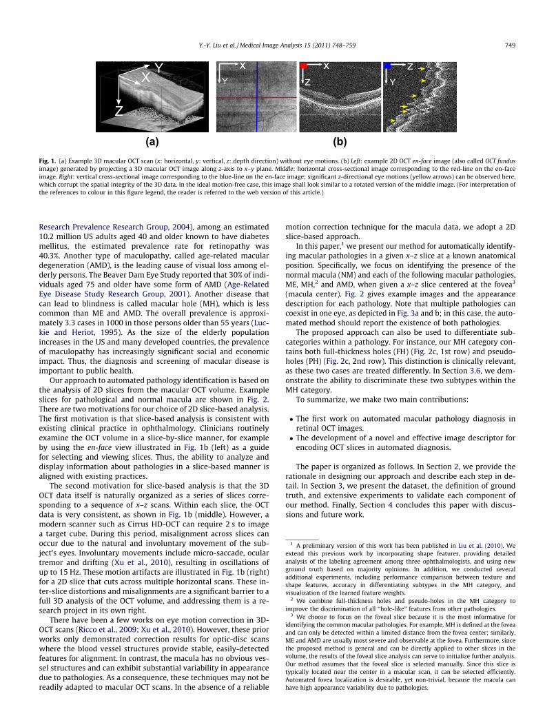
(a) (b)Fig. 1. (a) Example 3D macular OCT scan (x: horizontal, y: vertical, z: depth direction) without eye motions. (b) Left: example 2D OCT en-face image (also called OCT fundusimage) generated by projecting a 3D macular OCT image along z-axis to x–y plane. Middle: horizontal cross-sectional image corresponding to the red-line on the en-faceimage. Right: vertical cross-sectional image corresponding to the blue-line on the en-face image; significant z-directional eye motions (yellow arrows) can be observed here,which corrupt the spatial integrity of the 3D data. In the ideal motion-free case, this image shall look similar to a rotated version of the middle image. (For interpretation ofthe references to colour in this figure legend, the reader is referred to the web version of this article.)

1 A preliminary version of this work has been published in Liu et al. (2010). Weextend this previous work by incorporating shape features, providing detailedanalysis of the labeling agreement among three ophthalmologists, and using newground truth based on majority opinions. In addition, we conducted severaladditional experiments, including performance comparison between texture andshape features, accuracy in differentiating subtypes in the MH category, andvisualization of the learned feature weights.

2 We combine full-thickness holes and pseudo-holes in the MH category toimprove the discrimination of all ‘‘hole-like’’ features from other pathologies.

3 We choose to focus on the foveal slice because it is the most informative foridentifying the common macular pathologies. For example, MH is defined at the foveaand can only be detected within a limited distance from the fovea center; similarly,ME and AMD are usually most severe and observable at the fovea. Furthermore, sincethe proposed method is general and can be directly applied to other slices in thevolume, the results of the foveal slice analysis can serve to initialize further analysis.Our method assumes that the foveal slice is selected manually. Since this slice istypically located near the center in a macular scan, it can be selected efficiently.Automated fovea localization is desirable, yet non-trivial, because the macula canhave high appearance variability due to pathologies.

Y.-Y. Liu et al. / Medical Image Analysis 15 (2011) 748–759 749

Research Prevalence Research Group, 2004), among an estimated10.2 million US adults aged 40 and older known to have diabetesmellitus, the estimated prevalence rate for retinopathy was40.3%. Another type of maculopathy, called age-related maculardegeneration (AMD), is the leading cause of visual loss among el-derly persons. The Beaver Dam Eye Study reported that 30% of indi-viduals aged 75 and older have some form of AMD (Age-RelatedEye Disease Study Research Group, 2001). Another disease thatcan lead to blindness is called macular hole (MH), which is lesscommon than ME and AMD. The overall prevalence is approxi-mately 3.3 cases in 1000 in those persons older than 55 years (Luc-kie and Heriot, 1995). As the size of the elderly populationincreases in the US and many developed countries, the prevalenceof maculopathy has increasingly significant social and economicimpact. Thus, the diagnosis and screening of macular disease isimportant to public health.

Our approach to automated pathology identification is based onthe analysis of 2D slices from the macular OCT volume. Exampleslices for pathological and normal macula are shown in Fig. 2.There are two motivations for our choice of 2D slice-based analysis.The first motivation is that slice-based analysis is consistent withexisting clinical practice in ophthalmology. Clinicians routinelyexamine the OCT volume in a slice-by-slice manner, for exampleby using the en-face view illustrated in Fig. 1b (left) as a guidefor selecting and viewing slices. Thus, the ability to analyze anddisplay information about pathologies in a slice-based manner isaligned with existing practices.

The second motivation for slice-based analysis is that the 3DOCT data itself is naturally organized as a series of slices corre-sponding to a sequence of x–z scans. Within each slice, the OCTdata is very consistent, as shown in Fig. 1b (middle). However, amodern scanner such as Cirrus HD-OCT can require 2 s to imagea target cube. During this period, misalignment across slices canoccur due to the natural and involuntary movement of the sub-ject’s eyes. Involuntary movements include micro-saccade, oculartremor and drifting (Xu et al., 2010), resulting in oscillations ofup to 15 Hz. These motion artifacts are illustrated in Fig. 1b (right)for a 2D slice that cuts across multiple horizontal scans. These in-ter-slice distortions and misalignments are a significant barrier to afull 3D analysis of the OCT volume, and addressing them is a re-search project in its own right.

There have been a few works on eye motion correction in 3D-OCT scans (Ricco et al., 2009; Xu et al., 2010). However, these priorworks only demonstrated correction results for optic-disc scanswhere the blood vessel structures provide stable, easily-detectedfeatures for alignment. In contrast, the macula has no obvious ves-sel structures and can exhibit substantial variability in appearancedue to pathologies. As a consequence, these techniques may not bereadily adapted to macular OCT scans. In the absence of a reliable

motion correction technique for the macula data, we adopt a 2Dslice-based approach.

In this paper,1 we present our method for automatically identify-ing macular pathologies in a given x–z slice at a known anatomicalposition. Specifically, we focus on identifying the presence of thenormal macula (NM) and each of the following macular pathologies,ME, MH,2 and AMD, when given a x–z slice centered at the fovea3

(macula center). Fig. 2 gives example images and the appearancedescription for each pathology. Note that multiple pathologies cancoexist in one eye, as depicted in Fig. 3a and b; in this case, the auto-mated method should report the existence of both pathologies.

The proposed approach can also be used to differentiate sub-categories within a pathology. For instance, our MH category con-tains both full-thickness holes (FH) (Fig. 2c, 1st row) and pseudo-holes (PH) (Fig. 2c, 2nd row). This distinction is clinically relevant,as these two cases are treated differently. In Section 3.6, we dem-onstrate the ability to discriminate these two subtypes within theMH category.

To summarize, we make two main contributions:

� The first work on automated macular pathology diagnosis inretinal OCT images.� The development of a novel and effective image descriptor for

encoding OCT slices in automated diagnosis.

The paper is organized as follows. In Section 2, we provide therationale in designing our approach and describe each step in de-tail. In Section 3, we present the dataset, the definition of groundtruth, and extensive experiments to validate each component ofour method. Finally, Section 4 concludes this paper with discus-sions and future work.

Fig. 2. Characteristics of (a) normal macula (NM): a smooth depression shows at the center (fovea), (b) macular edema (ME): retinal thickening and liquid accumulationappears as black blobs around the fovea, (c) macular hole (MH): a full-thickness hole (FH, 1st row) or pseudo hole (PH, 2nd row) formation at the fovea; for PH, the holeformation does not reach the outer most retinal layer (retinal pigment epitherium, RPE), (d) age-related macular degeneration (AMD): irregular contours usually extrude indome shapes appear at the bottom layer (RPE) of the retina.

Fig. 3. Example x–z (horizontal) slice with (a) MH (red) and ME (green), (b) ME(green) and AMD (blue), (c) a detached tissue, (d) shadowing effects. (Forinterpretation of the references to colour in this figure legend, the reader isreferred to the web version of this article.)

750 Y.-Y. Liu et al. / Medical Image Analysis 15 (2011) 748–759

2. Approach

Automated pathology identification in ocular OCT images iscomplicated by four factors. First, the co-existence of multiplepathologies (see Fig. 3a and b) or other pathological changes(e.g., detached membrane, see Fig. 3c) can confound the overallappearance, making it hard to model each pathology separately.Second, there is high variability in shape, size, and magnitudewithin the same pathology. In MH, for examples, the holes canhave different widths, depths, and shapes, and some can even becovered by incompletely detached tissues (the 4th example in

Fig. 2c), making explicit pathology modeling difficult. Third, themeasurement of reflectivity of the retina is affected by the opticalproperties of the overlying tissues (Schuman et al., 2004), e.g.,blood vessels will absorb much of the transmitted light and opaquemedia will block the light, and thus produce shadowing effects(Fig. 3d). Fourth, a portion of the image may have lower qualitydue to imperfect imaging (Barnum et al., 2008). As a result of theabove factors, attempting to hand-craft a set of features or rulesto identify each pathology separately is unlikely to succeed. In-stead, we propose to use machine learning techniques to automat-ically discover discriminative features from a set of trainingexamples.

Our analysis approach consists of three steps, which are illus-trated in Fig. 4. First, image alignment is performed to reduce theappearance variation across scans. Second, we construct a globaldescriptor for the aligned image and its corresponding edge mapby computing spatially-distributed multi-scale texture and shapefeatures. Multi-scale spatial pyramid (MSSP) is used to encodethe global spatial organization of the retina. To encode each spatialblock in MSSP, we employ dimension-reduced local binary pattern(LBP) histogram (Ojala et al., 2002) to capture the texture andshape characteristics of the retinal image. This feature descriptorcan preserve the geometry as well as textures and shapes of theretinal image at multiple scales and spatial granularities. The laststep is to train a 2-class non-linear Support Vector Machine(SVM) (Chang and Lin, 2001) for each pathology. We now describeeach step in more detail.

2.1. Retina alignment

Imaged retinas have large variations in their inclination angles,positions, and natural curvatures across scans, as shown in Fig. 2. Itis therefore desirable to roughly align the retinas to reduce these

Fig. 4. Stages of our approach.

Y.-Y. Liu et al. / Medical Image Analysis 15 (2011) 748–759 751

variations before constructing the feature representation. To thisend, we use a simple heuristic procedure to flatten the curvatureand center the retina: (1) threshold the original image (Fig. 4a)to detect most of the retina structures (Fig. 4b); (2) apply a medianfilter to remove noise and thin detached tissues (Fig. 4c); (3) findthe entire retina by using morphological closing and then opening;by closing, we fill-up black blobs (e.g. cystoid edema) inside theretina, and by opening, we remove thin or small objects outsidethe retina (Fig. 4d); (4) fit the found retina area with a second-order polynomial using least-square curve fitting (Fig. 4e); wechoose a low order polynomial to avoid overfitting, and thus pre-serve important shape changes caused by pathologies; (5) warpthe entire retina to be approximately horizontal by translatingeach image column a distance according to the fitted curve(Fig. 4f) (after the warping, the fitted curve will become a horizon-tal line); then, crop the warped retina in the z-direction with areserved margin (see aligned result in Fig. 4). The exact parametervalues used in our procedure are presented in Section 3.2.

Note that our procedure fits and warps the entire retina ratherthan segmenting a particular retinal layer first (e.g. the RPE layer)and then performing flattening using that layer (Quellec et al.,2010). Our approach is motivated by the fact that the state of theart methods for layer segmentation are unreliable for scans withpathologies (Ishikawa et al., 2009). In the next section, we describean approach to spatially-redundant feature encoding which pro-vides robustness against any remaining variability in the alignedscans.

2.2. Multi-scale spatial pyramid (MSSP)

There are three motivations for our choice of a global spatially-distributed feature representation for OCT imagery based on MSSP.First, pathologies are often localized to specific retinal areas, mak-ing it important to encode spatial location. Second, the contextprovided by the overall appearance of the retina is important forcorrect interpretation; e.g., in Fig. 3d, we can distinguish betweena shadow and a macular hole more effectively given the context ofthe entire slice. Third, pathologies can exhibit discriminating char-acteristics at both small and large scales; therefore, both micro-patterns and macro-patterns should be represented. For these rea-sons, we use a global multi-scale image representation which pre-serves spatial organization.

We propose to use the multi-scale version of spatial pyramid(SP) (Lazebnik et al., 2006), denoted as MSSP, to capture the geom-etry of the aligned retina at multiple scales and spatial resolutions.

This global framework, MSSP, was recently proposed in Wu andRehg (2008), where it was successfully applied to challengingscene classification tasks. Fig. 5 illustrates the differences betweena 3-level MSSP and a 3-level SP. To form a k-level MSSP, for eachlevel l(0 6 l 6 (k � 1)), we rescale the original image by 2l�k+1 usingbilinear interpolation, and divide the rescaled image into 2l blocksin both image dimensions. The local features computed from allspatial blocks are concatenated in a predefined order to form anoverall global descriptor, as illustrated in Fig. 4. Note that we alsoadd the features from the overlapped blocks (the green blocks inFig. 5) to reduce boundary effects.

2.3. Histogram of LBP and dimensionality reduction using PCA

Local binary pattern (LBP) (Ojala et al., 2002) is a non-paramet-ric kernel which summarizes the local structure around a pixel. LBPis known to be highly discriminative and has been successfully ap-plied to computer vision tasks, such as texture classification (Ojalaet al., 2002), face recognition (Ahonen et al., 2006), and scene clas-sification (Wu and Rehg, 2008). It has also been effective in medicalimage analysis, such as texture classification in lung CT images(Sørensen et al., 2008), and false positive reduction in mammo-graphic mass detection (Oliver et al., 2007).

While there are several types of LBP, we follow (Ahonen et al.,2006; Oliver et al., 2007; Sørensen et al., 2008) in adopting LBP8,1

to capture the micro-patterns that reside in each local block. TheLBP8,1 operator derives an 8 bit binary code by comparing the cen-ter pixel to each of its 8 nearest neighbors in a 3 � 3 neighborhood,while ‘‘1’’ represents radius 1 when sampling the neighbors. Theresulting 8 bits are concatenated circularly to form an LBP codein the range [0255]. The computation is illustrated in Fig. 6a. Theformal equation can be written as:

LBP8;1 ¼X7

n¼0

f ðvn � vcÞ2n

where f(x) = 1 if x P 0, otherwise f(x) = 0; vc and vn represent thepixel value at the center and the neighboring pixel, respectively,with each neighbor being indexed circularly.

For each block of pixels in the MSSP, we compute the histogramof LBP codes to encode the statistical distribution of different mi-cro-patterns, such as spots, edges, corners, and flat areas. Histo-gram descriptors have proven to be effective at aggregating localintensity patterns into global discriminative features. In particular,they avoid the need to precisely localize discriminating imagestructures, which is difficult in complex and highly variable OCT

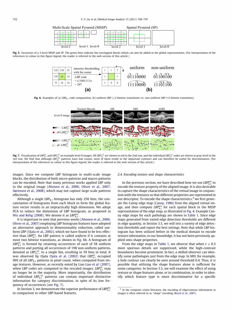
Fig. 5. Structures of a 3-level MSSP and SP. The green lines indicate the overlapped blocks which can also be added in the global representation. (For interpretation of thereferences to colour in this figure legend, the reader is referred to the web version of this article.)

(a) (b)Fig. 6. Examples of (a) LBP8,1 code computation, (b) uniform LBP (62 bitwise transitions) vs. non-uniform LBP (>2 bitwise transitions).

Fig. 7. Visualization of LBPu28;1 and LBP:u2

8;1 on example level-0 images. All LBP:u28;1 are shown in red in the 2nd row, and the individual LBP:u2

8;1 codes are shown in gray-level in the3rd row. We find that although LBP:u2

8;1 patterns have low counts, most of them reside in the important contours and can therefore be useful for discrimination. (Forinterpretation of the references to colour in this figure legend, the reader is referred to the web version of this article.)

4 In the computer vision literature, the encoding of edge/contour information inages is often referred to as ‘‘shape’’ encoding (Bosch et al., 2007).

752 Y.-Y. Liu et al. / Medical Image Analysis 15 (2011) 748–759

images. Since we compute LBP histogram in multi-scale imageblocks, the distribution of both micro-patterns and macro-patternscan be encoded. Note that many previous works applied LBP onlyin the original image (Ahonen et al., 2006; Oliver et al., 2007;Sørensen et al., 2008), which may not capture large-scale patternseffectively.

Although a single LBP8,1 histogram has only 256 bins, the con-catenation of histograms from each block to form the global fea-ture vector results in an impractically high dimension. We adoptPCA to reduce the dimension of LBP histogram, as proposed inWu and Rehg (2008). We denote it as LBPpca

8;1 .It is important to note that previous works (Ahonen et al., 2006;

Oliver et al., 2007) employing LBP histogram features have adoptedan alternative approach to dimensionality reduction, called uni-form LBP (Ojala et al., 2002), which we have found to be less effec-tive than LBPpca

8;1 . An LBP pattern is called uniform if it contains atmost two bitwise transitions, as shown in Fig. 6b. A histogram ofLBPu2

8;1 is formed by retaining occurrences of each of 58 uniformpatterns and putting all occurrences of 198 non-uniform patterns,denoted as LBP:u2

8;1 , to a single bin, resulting in 59 bins in total. Itwas observed by Ojala Ojala et al. (2002) that LBPu2

8;1 occupied90% of all LBP8,1 patterns in pixel count, when computed from im-age textures. However, as recently noted by Liao Liao et al. (2007),when LBP codes are computed in the rescaled images, LBPu2

8;1 mayno longer be in the majority. More importantly, the distributionof individual LBP:u2

8;1 patterns can contain important distinctiveinformation for category discrimination, in spite of its low fre-quency of occurrences (see Fig. 7).

In Section 3, we demonstrate the superior performance of LBPpca8;1

in comparison to other LBP-based features.

2.4. Encoding texture and shape characteristics

In the previous section, we have described how we use LBPpca8;1 to

encode the texture property of the aligned image. It is also desirableto capture the shape characteristics of the retinal image in conjunc-tion with the textures so that different properties are represented inour descriptor. To encode the shape characteristics,4 we first gener-ate the Canny edge map (Canny, 1986) from the aligned retinal im-age, and then compute LBPpca

8;1 for each spatial block in the MSSPrepresentation of the edge map, as illustrated in Fig. 4. Example Can-ny edge maps for each pathology are shown in Table 1. Since edgemaps generated from varied edge detection thresholds are differentin edge quantity, in Section 3.5, we will test a variety of edge detec-tion thresholds and report the best settings. Note that while LBP his-togram has been utilized before in the medical domain to encodetexture information, to our knowledge, it has not been previously ap-plied onto shape properties.

From the edge maps in Table 1, we observe that when t P 0.3most spurious details are suppressed, while the high-contrastboundaries become prominent. In fact, a skilled observer can iden-tify some pathologies just from the edge map. In MH, for example,a hole contour can clearly be seen around threshold 0.4. Thus, it ispossible that utilizing the shape features alone is sufficient forsome categories. In Section 3.5, we will examine the effect of usingtexture or shape features alone, or in combination, in order to iden-tify which feature type is more discriminative for a specific

im

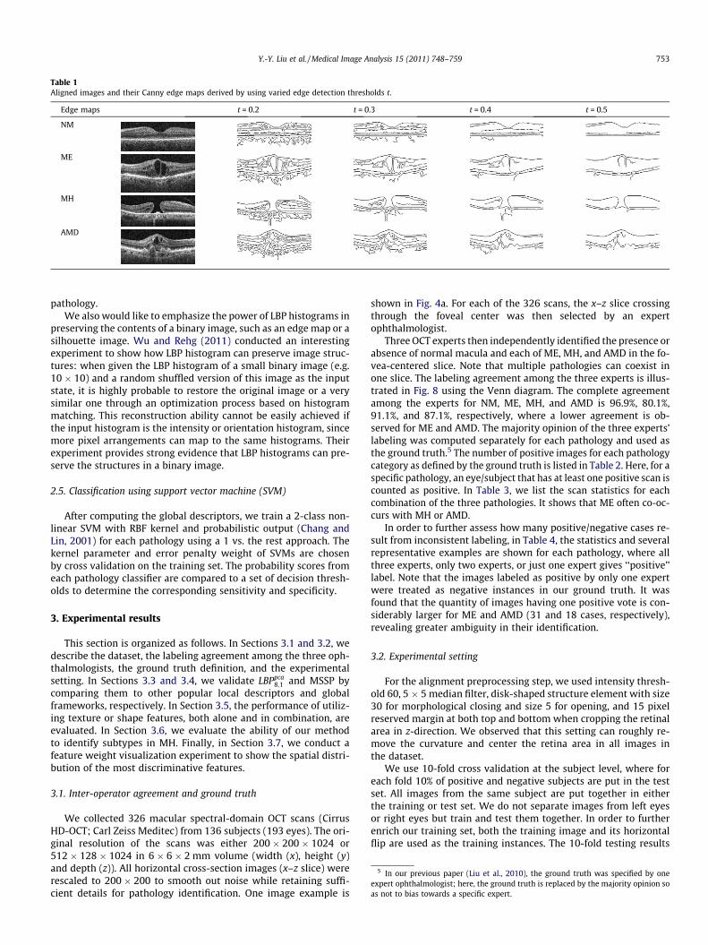
Table 1Aligned images and their Canny edge maps derived by using varied edge detection thresholds t.

Edge maps t = 0.2 t = 0.3 t = 0.4 t = 0.5

NM

ME

MH

AMD

5 In our previous paper (Liu et al., 2010), the ground truth was specified by oneexpert ophthalmologist; here, the ground truth is replaced by the majority opinion soas not to bias towards a specific expert.

Y.-Y. Liu et al. / Medical Image Analysis 15 (2011) 748–759 753

pathology.We also would like to emphasize the power of LBP histograms in

preserving the contents of a binary image, such as an edge map or asilhouette image. Wu and Rehg (2011) conducted an interestingexperiment to show how LBP histogram can preserve image struc-tures: when given the LBP histogram of a small binary image (e.g.10 � 10) and a random shuffled version of this image as the inputstate, it is highly probable to restore the original image or a verysimilar one through an optimization process based on histogrammatching. This reconstruction ability cannot be easily achieved ifthe input histogram is the intensity or orientation histogram, sincemore pixel arrangements can map to the same histograms. Theirexperiment provides strong evidence that LBP histograms can pre-serve the structures in a binary image.

2.5. Classification using support vector machine (SVM)

After computing the global descriptors, we train a 2-class non-linear SVM with RBF kernel and probabilistic output (Chang andLin, 2001) for each pathology using a 1 vs. the rest approach. Thekernel parameter and error penalty weight of SVMs are chosenby cross validation on the training set. The probability scores fromeach pathology classifier are compared to a set of decision thresh-olds to determine the corresponding sensitivity and specificity.

3. Experimental results

This section is organized as follows. In Sections 3.1 and 3.2, wedescribe the dataset, the labeling agreement among the three oph-thalmologists, the ground truth definition, and the experimentalsetting. In Sections 3.3 and 3.4, we validate LBPpca

8;1 and MSSP bycomparing them to other popular local descriptors and globalframeworks, respectively. In Section 3.5, the performance of utiliz-ing texture or shape features, both alone and in combination, areevaluated. In Section 3.6, we evaluate the ability of our methodto identify subtypes in MH. Finally, in Section 3.7, we conduct afeature weight visualization experiment to show the spatial distri-bution of the most discriminative features.

3.1. Inter-operator agreement and ground truth

We collected 326 macular spectral-domain OCT scans (CirrusHD-OCT; Carl Zeiss Meditec) from 136 subjects (193 eyes). The ori-ginal resolution of the scans was either 200 � 200 � 1024 or512 � 128 � 1024 in 6 � 6 � 2 mm volume (width (x), height (y)and depth (z)). All horizontal cross-section images (x–z slice) wererescaled to 200 � 200 to smooth out noise while retaining suffi-cient details for pathology identification. One image example is

shown in Fig. 4a. For each of the 326 scans, the x–z slice crossingthrough the foveal center was then selected by an expertophthalmologist.

Three OCT experts then independently identified the presence orabsence of normal macula and each of ME, MH, and AMD in the fo-vea-centered slice. Note that multiple pathologies can coexist inone slice. The labeling agreement among the three experts is illus-trated in Fig. 8 using the Venn diagram. The complete agreementamong the experts for NM, ME, MH, and AMD is 96.9%, 80.1%,91.1%, and 87.1%, respectively, where a lower agreement is ob-served for ME and AMD. The majority opinion of the three experts’labeling was computed separately for each pathology and used asthe ground truth.5 The number of positive images for each pathologycategory as defined by the ground truth is listed in Table 2. Here, for aspecific pathology, an eye/subject that has at least one positive scan iscounted as positive. In Table 3, we list the scan statistics for eachcombination of the three pathologies. It shows that ME often co-oc-curs with MH or AMD.

In order to further assess how many positive/negative cases re-sult from inconsistent labeling, in Table 4, the statistics and severalrepresentative examples are shown for each pathology, where allthree experts, only two experts, or just one expert gives ‘‘positive’’label. Note that the images labeled as positive by only one expertwere treated as negative instances in our ground truth. It wasfound that the quantity of images having one positive vote is con-siderably larger for ME and AMD (31 and 18 cases, respectively),revealing greater ambiguity in their identification.

3.2. Experimental setting

For the alignment preprocessing step, we used intensity thresh-old 60, 5 � 5 median filter, disk-shaped structure element with size30 for morphological closing and size 5 for opening, and 15 pixelreserved margin at both top and bottom when cropping the retinalarea in z-direction. We observed that this setting can roughly re-move the curvature and center the retina area in all images inthe dataset.

We use 10-fold cross validation at the subject level, where foreach fold 10% of positive and negative subjects are put in the testset. All images from the same subject are put together in eitherthe training or test set. We do not separate images from left eyesor right eyes but train and test them together. In order to furtherenrich our training set, both the training image and its horizontalflip are used as the training instances. The 10-fold testing results

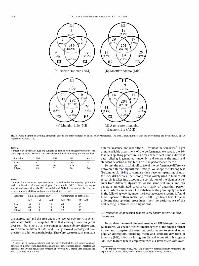
Fig. 8. Venn diagram of labeling agreement among the three experts on all macular pathologies. The actual scan numbers and the percentages are both shown. E1–E3represents experts 1–3.

Table 2Number of positive scans, eyes and subjects, as defined by the majority opinion of thethree experts. Note that each scan was labeled with all coinciding macular findings.

Statistics NM MH ME AMD

Scan 81 74 203 74Eye 66 36 116 37Subject 65 33 90 26

Table 3Number of positive scans, eyes and subjects as defined by the majority opinion foreach combination of three pathologies. For example, ‘‘MH’’ column representsstatistics of scans with only MH, but no ME and AMD. In our dataset, there are noscans containing all three pathologies, although it is possible.

Statistics Single pathology only Combination of pathologies

ME MH AMD ME + MH ME + AMD

Scan 93 9 29 65 45Eye 65 3 15 34 25Subject 53 3 13 32 19

754 Y.-Y. Liu et al. / Medical Image Analysis 15 (2011) 748–759

are aggregated6 and the area under the receiver operator character-istic curve (AUC) is computed. Note that although some subjects/eyes contribute more than one scan in our image library, these scanswere taken on different dates and usually showed pathological pro-gression or additional pathologies. Therefore, we treat each scan as a

6 Since the 10-fold data splitting is at the subject level while each subject can havedifferent number of scans, each fold can have quite different scan count. Therefore, weaggregate the 10-fold results and compute one overall AUC, rather than deriving theAUC separately for each fold.

different instance, and report the AUC result at the scan level.7 To geta more reliable assessment of the performance, we repeat the 10-fold data splitting procedure six times, where each time a differentdata splitting is generated randomly, and compute the mean andstandard deviation of the 6 AUCs as the performance metric.

To test the statistical significance of the performance differencebetween different algorithmic settings, we adopt the DeLong test(DeLong et al., 1988) to compare their receiver operating charac-teristic (ROC) curves. The DeLong test is widely used in biomedicalresearch. It takes into account the correlation of the diagnostic re-sults from different algorithms for the same test units, and cangenerate an estimated covariance matrix of algorithm perfor-mance, which can be used for statistical testing. We apply the testin the following way: if, under the DeLong test, one setting is foundto be superior to than another at p = 0.05 significant level for all 6different data-splitting procedures, then the performance of thebest setting is claimed to be significant.

3.3. Validation of dimension-reduced local binary patterns as localdescriptors

To validate the use of dimension-reduced LBP histograms as lo-cal features, we encode the texture properties of the aligned retinalimage, and compare the resulting performance to several otherpopular descriptors, including mean and standard deviation ofintensity (MS), intensity histogram (I), and orientation histogram(O). Each feature type is employed with a 3-level MSSP with over-

7 In our prior work (Liu et al., 2010), we did subject normalization in computing thexperimental results. Here, the scan level accuracy is directly reported.

e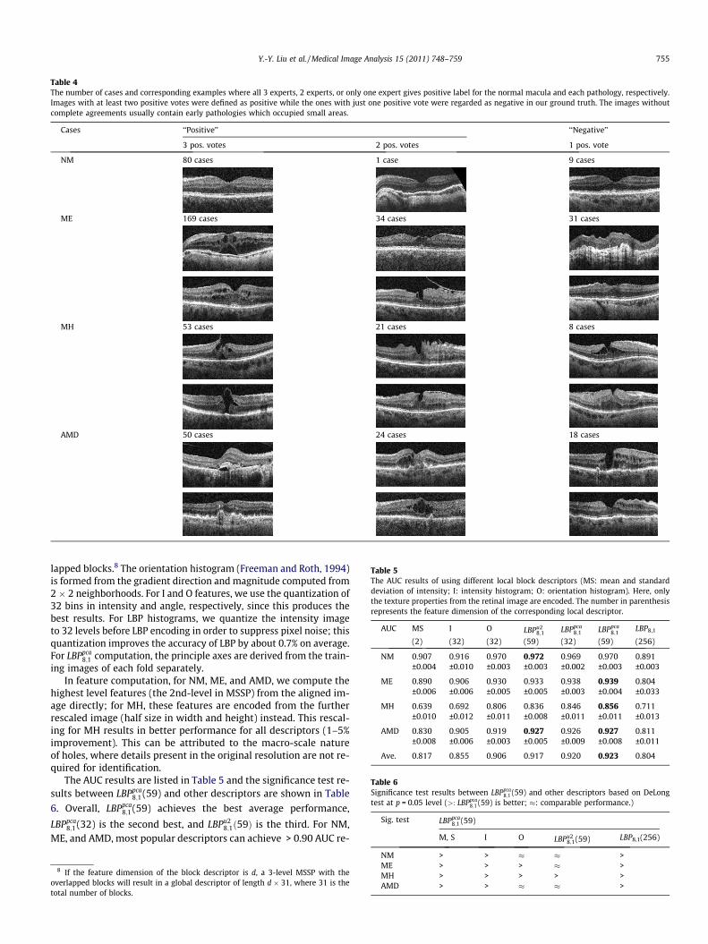

Table 4The number of cases and corresponding examples where all 3 experts, 2 experts, or only one expert gives positive label for the normal macula and each pathology, respectively.Images with at least two positive votes were defined as positive while the ones with just one positive vote were regarded as negative in our ground truth. The images withoutcomplete agreements usually contain early pathologies which occupied small areas.

Cases ‘‘Positive’’ ‘‘Negative’’

3 pos. votes 2 pos. votes 1 pos. vote

NM 80 cases 1 case 9 cases

ME 169 cases 34 cases 31 cases

MH 53 cases 21 cases 8 cases

AMD 50 cases 24 cases 18 cases

Table 5The AUC results of using different local block descriptors (MS: mean and standarddeviation of intensity; I: intensity histogram; O: orientation histogram). Here, onlythe texture properties from the retinal image are encoded. The number in parenthesisrepresents the feature dimension of the corresponding local descriptor.

AUC MS I O LBPu28;1 LBPpca

8;1 LBPpca8;1

LBP8,1

(2) (32) (32) (59) (32) (59) (256)

NM 0.907 0.916 0.970 0.972 0.969 0.970 0.891±0.004 ±0.010 ±0.003 ±0.003 ±0.002 ±0.003 ±0.003

ME 0.890 0.906 0.930 0.933 0.938 0.939 0.804±0.006 ±0.006 ±0.005 ±0.005 ±0.003 ±0.004 ±0.033

MH 0.639 0.692 0.806 0.836 0.846 0.856 0.711±0.010 ±0.012 ±0.011 ±0.008 ±0.011 ±0.011 ±0.013

AMD 0.830 0.905 0.919 0.927 0.926 0.927 0.811±0.008 ±0.006 ±0.003 ±0.005 ±0.009 ±0.008 ±0.011

Ave. 0.817 0.855 0.906 0.917 0.920 0.923 0.804

Table 6Significance test results between LBPpca

8;1 (59) and other descriptors based on DeLongtest at p = 0.05 level (>: LBPpca

8;1 (59) is better; �: comparable performance.)

Sig. test LBPpca8;1 (59)

M, S I O LBPu28;1(59) LBP8,1(256)

Y.-Y. Liu et al. / Medical Image Analysis 15 (2011) 748–759 755

lapped blocks.8 The orientation histogram (Freeman and Roth, 1994)is formed from the gradient direction and magnitude computed from2 � 2 neighborhoods. For I and O features, we use the quantization of32 bins in intensity and angle, respectively, since this produces thebest results. For LBP histograms, we quantize the intensity imageto 32 levels before LBP encoding in order to suppress pixel noise; thisquantization improves the accuracy of LBP by about 0.7% on average.For LBPpca

8;1 computation, the principle axes are derived from the train-ing images of each fold separately.

In feature computation, for NM, ME, and AMD, we compute thehighest level features (the 2nd-level in MSSP) from the aligned im-age directly; for MH, these features are encoded from the furtherrescaled image (half size in width and height) instead. This rescal-ing for MH results in better performance for all descriptors (1–5%improvement). This can be attributed to the macro-scale natureof holes, where details present in the original resolution are not re-quired for identification.

The AUC results are listed in Table 5 and the significance test re-sults between LBPpca

8;1 (59) and other descriptors are shown in Table

6. Overall, LBPpca8;1 (59) achieves the best average performance,

LBPpca8;1 (32) is the second best, and LBPu2

8;1ð59Þ is the third. For NM,ME, and AMD, most popular descriptors can achieve > 0.90 AUC re-

8 If the feature dimension of the block descriptor is d, a 3-level MSSP with theoverlapped blocks will result in a global descriptor of length d � 31, where 31 is thetotal number of blocks.

NM > > � � >ME > > > � >MH > > > > >AMD > > � � >

Table 7The AUC results of employing different global frameworks (MSSP: multi-scale spatial pyramid; SP: spatial pyramid; SD: single 2nd-level spatial division; ‘‘nO’’: exclude theoverlapped blocks) with LBPpca

8;1 (32) as the local descriptors. Here, only the texture properties from the retinal image are encoded. Significance test results are in the last columnbased on DeLong test at p = 0.05 level (>: left setting is better; �: comparable performance).

AUC MSSP SP SD MSSPnO SPnO SDnO Sig. Test

NM 0.969 0.963 0.965 0.963 0.957 0.961 MSSP � SP, SL±0.002 ±0.003 ±0.002 ±0.002 ±0.004 ±0.003

ME 0.938 0.930 0.927 0.942 0.933 0.930 MSSP � SP, SL±0.003 ±0.005 ±0.004 ±0.001 ±0.005 ±0.003

MH 0.846 0.817 0.825 0.839 0.804 0.814 MSSP > SP, SL±0.011 ±0.013 ±0.010 ±0.015 ±0.014 ±0.012

AMD 0.926 0.903 0.908 0.911 0.872 0.866 MSSP > SP, SL±0.009 ±0.007 ±0.007 ±0.009 ±0.011 ±0.014

Ave. 0.920 0.903 0.906 0.913 0.892 0.893

0.88

0.89

0.9

0.91

0.92

0.93

0.94

0.95

0.96

0.97

0.98

0.2 0.3 0.4 0.5

AU

C

Edge Detection Threshold (t)

NM (S)

NM (T+S)

ME (S)

ME (T+S)

MH (S)

MH (T+S)

AMD (S)

AMD (T+S)

Fig. 9. AUC results with respect to varied edge detection thresholds t when using Sand TS features, respectively. MH is more sensitive to the settings of t than the othercategories.

Table 8The AUC results of different feature types (T: texture, S: shape, TS: texture + shape)under the best edge detection threshold t, all with LBPpca

8;1 (32) as the local descriptors.Significance test results are in the last column based on DeLong test at p = 0.05 level(>: left setting is better; �: comparable performance).

AUC T S TS Sig. test

NM 0.969 0.971 (t = 0.4) 0.976 (t = 0.4) T � S, TS > T, TS � S±0.002 ±0.002 ±0.002

ME 0.939 0.923 (t = 0.3) 0.939 (t = 0.4) T > S, TS � T, TS > S±0.004 ±0.005 ±0.004

MH 0.846 0.931 (t = 0.4) 0.919 (t = 0.4) S > T, TS > T, TS � S±0.011 ±0.005 ±0.005

AMD 0.925 0.931 (t = 0.2) 0.938 (t = 0.2) T � S � TS±0.008 ±0.005 ±0.006

Ave. 0.920 0.939 0.943

Table 9The number of scans, eyes and subjects as defined by one expertophthalmologist for full-thickness hole (FH) and pseudo-hole(PH) in MH category.

Statistics FH PH

Scan 39 35Eye 17 15Subject 17 18

0.91

0.92

0.93

0.94

0.95

0.96

0.2 0.3 0.4 0.5

AU

C

Edge Detection Threshold (t)

FH/PH (S)

FH/PH (T+S)

Fig. 10. The AUC results with respect to varied edge detection thresholds (t) whenusing S and TS features for discriminating FH and PH.

Table 10The AUC results in discriminating FH and PH in MH category using differentcombination of feature types (T: texture, S: shape, TS: texture + shape) all withLBPpca

8;1 (32) as the local descriptors. Significance test results are in the last columnbased on DeLong test at p = 0.05 level (>: left setting is better; �: comparableperformance).

AUC T S TS Sig. test

FH vs. PH 0.871 0.946 (t = 0.2) 0.951 (t = 0.2) S > T, TS > T, S � TS±0.015 ±0.011 ±0.011

9 Only 4 � 4 = 16 spatial blocks derived from the original image were used.

756 Y.-Y. Liu et al. / Medical Image Analysis 15 (2011) 748–759

sults, but for MH, the AUC is much lower for all (the best is 0.856from LBPpca

8;1 (59)). In detail, both LBPu28;1ð59Þ and LBPpca

8;1 ð59Þ performsignificantly better than MS and I for all categories. When com-pared to O, LBPpca

8;1 ð59Þ is comparable for NM and AMD, but is signif-

icantly better for ME and MH. For MH, LBPpca8;1 (59) outperforms O by

5% and by an even larger margin for MS and I. This can be attrib-uted to LBPpca

8;1 ’s highly discriminative ability in preserving macularhole structures, while other features with smaller neighborhoodsdo not possess. Also note that the use of all 256 bins of LBP histo-gram gives the worst results, presumably due to overfitting in thehigh dimensional feature space.

We then compare the results of LBPu28;1ð59Þ and LBPpca

8;1 ð59Þ. FromTables 5 and 6, these two settings have comparable performancefor NM, ME, and AMD, but for MH, LBPpca

8;1 ð59Þ is significantly better

than LBPu28;1ð59Þ. This shows that the removal of individual non-uni-

form patterns, as used in LBPu28;1ð59Þ, can result in the loss of impor-

tant discriminative information. Finally, we found that the use ofthe first 32 principal components ðLBPpca

8;1 ð32ÞÞ seems sufficientfor NM, ME, and AMD identification.

In the following sections, we adopt LBPpca8;1 (32) as the local

descriptors for all pathologies.

3.4. Validation of multi-scale spatial pyramid as global representation

In Table 7, we compare the performance of a 3-level MSSP witha 3-level spatial pyramid (SP) and a single 2nd-level spatial divi-sion (SD),9 all with and without the overlapped blocks (‘‘without’’denoted as ‘‘nO’’). Overall, the proposed MSSP achieves the best per-

Fig. 11. Visualization of feature weights of trained linear SVMs for each pathology. The block weights are rescaled to [0 255] for better visualization, with the brightest oneenclosed by a red rectangle. (The feature setting is TS (t = 0.4) for NM, T for ME, S (t = 0.4) for MH, TS (t = 0.2) for AMD, and S (t = 0.2) for FH/PH). (For interpretation of thereferences to colour in this figure legend, the reader is referred to the web version of this article.)

Y.-Y. Liu et al. / Medical Image Analysis 15 (2011) 748–759 757

formance. In MH and AMD category, MSSP outperforms SP and SL bya large margin, which clearly shows the benefit of multi-scale mod-eling. When features from the overlapped blocks are removed (‘‘nO’’),the performance of all frameworks are considerably lower for AMDand MH, which demonstrates the advantage of including the over-lapped blocks.

3.5. Evaluation of texture or shape features, both alone and incombination

In the previous sections, we have established that LBPpca8;1 and

MSSP are effective in encoding texture distribution in the retinalOCT images. We now evaluate the performance of different featuretypes–texture (T) alone, shape (S) alone, or in combination (TS). Forshape features, we test the performance of several edge detectionthresholds (t = 0.2,0.3, . . . ,0.5). The AUC results under different

edge detection thresholds t for S and TS are plotted in Fig. 9. Thebest AUC results achieved by each feature type are detailed inTable 8. For NM, ME, MH, and AMD, the best AUCs are 0.976,0.939, 0.931, and 0.938, derived from the feature type setting: TS(t = 0.4), T, S (t = 0.4), and TS (t = 0.2), respectively.

From Table 8, we find that for NM, TS significantly outperformsT though the absolute gain is small (0.7% in AUC); thus, includingshape features can provide additional useful information. For ME,T and TS are significantly better than using S alone (1.6% AUC dif-ference), but TS does not outperform T; this suggests that texturedescriptors alone, which describe the distribution of intensity pat-terns, are discriminative enough for edema detection, e.g., detec-tion of dark cystic areas embedded in lighter retinal layers. ForMH, S is significantly better than using T or TS, with a large AUCdifference (8.5%) between S and T. This reveals that using shapefeatures alone is sufficient to capture the distinct contours of

758 Y.-Y. Liu et al. / Medical Image Analysis 15 (2011) 748–759

MH, while the details present in texture features might distract theclassifier and harm the performance. For AMD, all three feature set-tings (T, S, TS) have no significant difference, but using combinedfeatures (TS) achieved the best performance, suggesting that bothfeatures types are beneficial.

Regarding the effects of edge detection thresholds t, in Fig. 9, wefind that for NM, ME, and AMD, the AUC results under different tare all within 1% in AUC; but for MH, the performance is muchmore sensitive to the choice of t. In MH, we can see an apparentpeak at t = 0.4, which retains relatively strong edges only, as shownin Table 1. When more weak edges are also included for MH(t < 0.4), the performance drops by a large margin (from 0.931 to0.888 when t decreases from 0.4 to 0.2). This suggests that includ-ing weak edges is harmful for identifying the hole structures.

3.6. Discrimination of sub-categories within MH category

We evaluated the performance of our method in discriminatingthe sub-categories, full-thickness holes (FH) and psedu-holes (PH),within MH category. The dataset statistics are listed in Table 9. TheAUC results under varied edge detection thresholds t are plotted inFig. 10. The best results for each feature type (T, S, TS) are detailedin Table 10.

In Table 10, we find that S and TS perform significantly betterthan T (>7% difference) while S and TS have no significant differ-ences. Again, for distinguishing different hole structures, shape fea-tures are much more effective than textures, the same as in theparent category (MH). Regarding the edge detection thresholds t,in Fig. 10, we discover that there is a local peak at t = 0.4, the sameas in MH category, but when t decreases to 0.2, the inclusion ofweaker edges can provide a performance leap. This suggests thatsubtle shape structures captured by these weak edges are usefulfor sub-category discrimination. Overall, the high AUC results(0.951) demonstrate that the proposed feature representation isalso effective at distinguishing similar-looking subtypes.

3.7. Visualization of feature weight distribution of linear SVMs

To gain insight into the characteristics of each pathology fromthe learning machine’s perspective, we conduct a visualizationexperiment to show the spatial distribution of the most discrimi-native features of the learned SVMs.

Our process and visualization scheme is as follows. For eachpathology, we train a linear SVM using one fold of the training dataand the best feature setting. After training, the weight value foreach feature entry is derived. Then, for each spatial block, we com-pute the block’s weight by summing up the absolute values ofweights from features belonging to the block. For better visualiza-tion, we then map the highest block weight to 255, and lowest to 0.The brightest block, which is deemed the most discriminative, isenclosed by a red rectangle. The results are shown in Fig. 11.

From Fig. 11, we find that the most discriminative blocks are lo-cated at different pyramid levels for different pathologies. We alsodiscover that for NM and ME, the brighter blocks are locatedaround the central and top areas, which are the places for the nor-mal, smooth depression or the hill shapes caused by the accumu-lated fluids. For MH, the top half areas, inhabited by the openingarea of the holes, get higher weights. For AMD, the middle and bot-tom areas are brighter, corresponding to the normal or irregularbottom retinal layer (RPE layer). For FH/PH, the area around thecentral bottom retinal layer, which is the place revealing whetherthe hole touches the outermost layer, is heavily weighted.

The distribution of these feature weights is consistent with ourintuition about the important areas for each pathology. This visu-alization experiment corroborates our initial hypothesis that SVMhas the ability to discover the most discriminative features when

given the full context, without the need for explicit feature selec-tion beforehand.

4. Conclusion and future work

In this paper, we present an effective data-driven approach toidentify normal macula and multiple macular pathologies, namely,ME, MH, and AMD, from the foveal slices in retinal OCT images.First, we align the slices to reduce their appearance variations.Then we construct a global image descriptor by using multi-scalespatial pyramid as the global representation, combined withdimension-reduced LBP histogram based on PCA as the localdescriptor to encode both the retinal image and its edge map. Thisapproach captures the geometry, texture, and shape of the retina ina principled way. A binary non-linear SVM classifier is then trainedfor each pathology to identify its presence. To further differentiatesubtypes within the MH category, our method is also applied todistinguish full-thickness holes from pseudo-holes. To our knowl-edge, our study is the first to automatically classify OCT imagesfor various macular pathologies.

Our feature representation is novel for medical image analysis.Although the LBP histogram has been applied in a variety of fields,to our knowledge, this is the first work using LBPpca descriptor, aswell as its use with the MSSP framework, in the medical domain.We have demonstrated that our feature representation outper-forms other popular choices. In addition, our use of LBPpca on theedge map for capturing the shape characteristics is the first seenin the medical literature. This shape encoding has proven to beeffective for MH identification.

We validate our approach by comparing its performance to thatof other commonly-used local descriptors and global representa-tions. We then examine the effectiveness of using texture andshape features alone, and in combination, for identifying eachpathology. We find that employing texture features alone is suffi-cient for ME while using shape features alone performs the bestfor identifying MH; for NM and AMD, utilizing both feature typesachieves the best performance. To gain more insight from a ma-chine learning perspective, we visualize the learned featureweights to study the spatial distribution of the learned most dis-criminative features. The pattern of the weights is consistent withour intuition regarding the spatial location of specific pathologies.Our results demonstrate the feasibility of a global feature encodingapproach which avoids the need to explicitly localize pathology-specific features within the OCT data.

Our method has several advantages. First, the histogram-basedimage features directly capture the statistical distribution ofappearance characteristics, resulting in objective measurementsand straightforward implementation. Second, the method is gen-eral, and can be extended to identify additional pathologies. Third,the same approach can be utilized to diagnose other cross sectionsbesides the foveal slices, as long as the corresponding labeled slicesfrom the desired anatomical locations are also gathered fortraining.

The present work has two limitations: We analyze a single fo-veal slice instead of the full 3D SD-OCT volume, and the target sliceis manually selected by expert ophthalmologists. While the fovealslice is the most informative one for identifying several commonmacular pathologies, analysis of the entire volume could be bene-ficial. In addition, such an approach could provide further utility byautomating the selection and presentation of relevant slices to theclinician.

In future work, we plan to extend the method to analyze eachslice in the entire macular cube. The most straightforward way isto train a set of y-indexed pathology classifiers, using labeled x–zslice sets from the same quantized y locations relative to the fovea.

Y.-Y. Liu et al. / Medical Image Analysis 15 (2011) 748–759 759

By using location-indexed classifiers, the normal and abnormalanatomical structures around similar y positions can be modeledmore accurately, and each slice from the entire cube can be exam-ined. Once the eye motion artifacts in the macular scans can bereliably corrected, we can further investigate the efficacy of volu-metric features in pathology identification. We also plan to developan automated method for fovea localization so that the entire pro-cess is fully-automatic.

In conclusion, an effective approach is proposed to computerizethe diagnosis of multiple macular pathologies in retinal OCTimages, which achieves AUC > 0.93 for all pathologies. Our methodcan be applied to diagnose every slice in the OCT volume. This mayprovide clinically-useful tools to support disease diagnosis,improving the efficiency of OCT-based ocular pathologyidentification.

Acknowledgements

This research is supported in part by National Institutes ofHealth contracts R01-EY013178 and P30-EY008098, The Eye andEar Foundation (Pittsburgh, PA), unrestricted grants from Researchto Prevent Blindness, Inc. (New York, NY), and grants from IntelLabs Pittsburgh (Pittsburgh, PA).

References

Age-Related Eye Disease Study Research Group, 2001. A randomized, placebo-controlled, clinical trial of high-dose supplementation with vitamins C and E,beta carotene, and zinc for age-related macular degeneration and vision loss:AREDS report no. 8. Arch Ophthalmol 119, pp. 1417–1436.

Ahonen, T., Hadid, A., Pietikäinen, M., 2006. Face description with local binarypatterns: application to face recognition. IEEE Transactions on Pattern Analysisand Machine Intelligence 28, 2037.

Barnum, P., Chen, M., Ishikawa, H., Wollstein, G., Schuman, J., 2008. Local qualityassessment for optical coherence tomography. In: IEEE InternationalSymposium on Biomedical Imaging, pp. 392–395.

Bosch, A., Zisserman, A., Munoz, X., 2007. Representing shape with a spatial pyramidkernel. In: ACM International Conference on Image and Video Retrieval, pp.401–408.

Canny, J., 1986. A computational approach to edge detection. IEEE Transactions onPattern Analysis and Machine Intelligence 8, 679–698.

Chang, C.C., Lin, C.J., 2001. LIBSVM: a library for support vector machines. <http://www.csie.ntu.edu.tw/cjlin/libsvm>.

DeLong, E., DeLong, D., Clarke-Pearson, D., 1988. Comparing the areas under two ormore correlated receiver operating characteristic curves: a nonparametricapproach. Biometrics 44, 837–845.

Freeman, W.T., Roth, M., 1994. Orientation histogram for hand gesture recognition.In: International Workshop on Automatic Face and Gesture Recognition, pp.296–301.

Garvin, M.K., Abràmoff, M.D., Kardon, R., Russell, S.R., Wu, X., Sonka, M., 2008.Intraretinal layer segmentation of macular optical coherence tomographyimages using optimal 3-D graph search. IEEE Transactions on Medical Imaging27, 1495.

Ishikawa, H., Kim, J.S., Friberg, T.R., Wollstein, G., Kagemann, L., Gabriele, M.L.,Townsend, K.A., Sung, K.R., Duker, J.S., Fujimoto, J.G., Schuman, J.S., 2009. Threedimensional optical coherence tomography (3D-OCT) image enhancement withsegmentation free contour modeling c-mode. Investigative Ophthalmology andVisual Science 50, 1344–1349.

Ishikawa, H., Stein, D.M., Wollstein, G., Beaton, S., Fujimoto, J.G., Schuman, J.S., 2005.Macular segmentation with optical coherence tomography. InvestigativeOphthalmology and Visual Science 46, 2012–2017.

Lazebnik, S., Schmid, C., Ponce, J., 2006. Beyond bags of features: spatial pyramidmatching for recognizing natural scene categories. In: IEEE Computer Visionand Pattern Recognition, pp. 2169–2178.

Lee, K., Niemeijer, M., Garvin, M.K., Kwon, Y.H., Sonka, M., Abramoff, M.D., 2010.Segmentation of the optic disc in 3-D OCT scans of the optic nerve head. IEEETransactions on Medical Imaging 29, 1321–1330.

Liao, S., Zhu, X., Lei, Z., Zhang, L., Li, S.Z., 2007. Learning multi-scale block localbinary patterns for face recognition. In: International Conference on Biometrics,vol. 4642, pp. 828–837.

Liu, Y.Y., Chen, M., Ishikawa, H., Wollstein, G., Schuman, J., Rehg, J.M., 2010.Automated macular pathology diagnosis in retinal OCT images using multi-scale spatial pyramid with local binary patterns. In: International Conference onMedical Image Computing and Computer Assisted Intervention, vol. 6361, pp.1–9.

Luckie, A., Heriot, W., 1995. Macular holes: pathogenesis, natural history, andsurgical outcomes. Australian and New Zealand Journal of Ophthalmology 23,93–100.

Ojala, T., Pietikäinen, M., Mäenpää, T., 2002. Multiresolution gray-scale and rotationinvariant texture classification with local binary patterns. IEEE Transactions onPattern Analysis and Machine Intelligence 24, 971.

Oliver, A., Lladó, X., Freixenet, J., Martí, J., 2007. False positive reduction inmammographic mass detection using local binary patterns. In: InternationalConference on Medical Image Computing and Computer Assisted Intervention,vol. 4791, pp. 286–293.

Quellec, G., Lee, L., Dolejsi, M., Garbvin, M.K., Abramoff, M.D., Sonka, M., 2010.Three-dimensional analysis of retinal layer texture: identification of fluid-filledregions in SD-OCT of the macula. IEEE Transactions on Med Imaging 29, 1321–1330.

Ricco, S., Chen, M., Ishikawa, H., Wollstein, G., Schuman, J.S., 2009. Correctingmotion artifacts in retinal spectral domain optical coherence tomography viaimage registration. In: International Conference on Medical Image Computingand Computer Assisted Intervention, vol. 5761, pp. 100–107.

Schuman, J., Pedut-Kloizman, T., Hertzmark, E., 1996. Reproducibility of nerve fiberlayer thickness measurements using optical coherence tomography.Ophthalmology 103, 1889–1898.

Schuman, J.S., Puliafito, C.A., Fujimoto, J.G., 2004. Optical Coherence Tomography ofOcular Diseases, second ed.

Srensen, L., Shaker, S.B., Bruijne, M.D., 2008. Texture classification in lung CT usinglocal binary patterns. In: International Conference on Medical Image Computingand Computer Assisted Intervention, vol. 5241, pp. 934–941.

The Eye Diseases Research Prevalence Research Group, 2004. The prevalence ofdiabetic retinopathy among adults in the United States. Archives ofOphthalmology 122, 552–563.

Wu, J., Rehg, J.M., 2008. Where am I: place instance and category recognition usingspatial PACT. In: IEEE Computer Vision and Pattern Recognition, pp. 1–8.

Wu, J., Rehg, J.M., 2011. CENTRIST: a visual descriptor for scene categorization. IEEETransactions on Pattern Analysis and Machine Intelligence 33, 1489–1501.

Xu, J., Ishikawa, H., Wollstein, G., Schuman, J.S., 2010. 3D OCT eye movementcorrection based on particle filtering. In: International Conference on IEEEEngineering in Medicine and Biology Society, pp. 53–56.