Embed Size (px)
Citation preview
i
Automated Investment Analysis
An Interactive Qualifying Project
Submitted to the Faculty
Of
Worcester Polytechnic Institute
In Partial Fulfillment of the requirements for
Degree of Bachelor of Science
By:
Ben Blakeslee
James Ham
Vanessa Guo
Submitted on May 30, 2011
Approved by: Professor Hossein Hakim, Advisor
ii
Abstract With the recent financial crisis in America, investors have received the bulk of the blame and
thus have been tasked with improving investment techniques to prevent another recession of such high
magnitude. Here we look to develop new methods for investing using preprogrammed algorithms that
automate the process of deciding whether to buy, sell, or avoid a stock. These algorithms use both
technical and fundamental data to improve investing success by removing the factor of human emotion
from trading, reducing risk of loss due to greed. We ultimately find that with a careful application of
technical and fundamental data, as well as a thorough understanding of common patterns in financial
markets, it is possible to develop an automated trading strategy that can profitably trade stocks and
currencies.

iii
Table of Contents Abstract ..................................................................................................................................................... ii
Tables ....................................................................................................................................................... vi
Figures ...................................................................................................................................................... vi
1. Introduction .......................................................................................................................................... 1
2. Project Description ................................................................................................................................ 2
3. Background Information ....................................................................................................................... 3
3.1 Investment Options......................................................................................................................... 3
3.2 Reading charts ................................................................................................................................. 5
3.3 Trading Terminology ....................................................................................................................... 8
3.4 Markets ......................................................................................................................................... 11
3.5 Automated Trading ....................................................................................................................... 13
3.6 Systems Trading ............................................................................................................................ 17
3.7 Fundamental Analysis ................................................................................................................... 23
3.8 Technical Analysis ......................................................................................................................... 31
3.9 Tradestation .................................................................................................................................. 49
4. Trading Plans, Journals, and Equity Charts ............................................................................................. 52
4.1 Trading Plan ...................................................................................................................................... 52
4.2 Trading Journal .................................................................................................................................. 52
4.3 Equity Charts ..................................................................................................................................... 52
5. Algorithm from Tradestation Labs .......................................................................................................... 53
5.1 Contrarian Z-Score Algorithm ........................................................................................................... 53
6. Slope Calculating Algorithm .................................................................................................................... 55
6.1 Overview ........................................................................................................................................... 55
6.2 Improvements ................................................................................................................................... 55
6.3 Conclusion ......................................................................................................................................... 60
7. Factor Weight Algorithm ......................................................................................................................... 62
7.1 Overview ........................................................................................................................................... 62
7.2 Factors Used ...................................................................................................................................... 62
7.3 Usage of the Algorithm ..................................................................................................................... 65
7.3.1 Equation Calculation .................................................................................................................. 65
7.3.2 Weight Parameter Estimation.................................................................................................... 67

iv
7.3.3 Equation Implementation .......................................................................................................... 70
7.4 Potential Errors ................................................................................................................................. 72
8. Indicator Scorecard Algorithm ................................................................................................................ 75
8.1 Overview ........................................................................................................................................... 75
8.2 Alternative Approach to Parameter Estimation ............................................................................... 77
8.3 Results ............................................................................................................................................... 79
8.4 Future Work ...................................................................................................................................... 79
9. Indicator Multi Test Algorithm ................................................................................................................ 80
10. ADX/Stochastics Algorithm ................................................................................................................... 82
10.1 Indicators used ................................................................................................................................ 82
10.2 Rules ................................................................................................................................................ 82
10.3 Performance ................................................................................................................................... 82
10.4 Conclusion ....................................................................................................................................... 84
11. Portfolio Algorithm ............................................................................................................................... 85
12. Historical Data Analysis: ........................................................................................................................ 88
12.1 Method ........................................................................................................................................... 88
12.2 Data analysis ................................................................................................................................... 90
12.2.1 Data body and wick range activity chart .................................................................................. 90
12.2.3 Analysis result .......................................................................................................................... 90
12.2.4 Correlation ............................................................................................................................... 91
12.3 Evaluation of Data ........................................................................................................................... 92
13. Active Time Analysis .............................................................................................................................. 93
Interval activity period explanation ............................................................................................................ 93
Body or Wick? ......................................................................................................................................... 93
Directly compare & STANDARDIZE ......................................................................................................... 93
14. Live Trading ........................................................................................................................................... 97
14.1 Bid and Ask Prices ........................................................................................................................... 97
14.2 Intra Bar Data .................................................................................................................................. 98
14.3 Constant Operation ......................................................................................................................... 98
14.4 Results ............................................................................................................................................. 99
15. Conclusion ........................................................................................................................................... 100
15.1 Future Work .................................................................................................................................. 100
v
15.2 Suggestions ................................................................................................................................... 100
16. References .......................................................................................................................................... 102
Works Cited ............................................................................................................................................... 102
17. Appendix ............................................................................................................................................. 104
Appendix 1 – Table of Monthly Correlation .......................................................................................... 104
Appendix 2 – Table of Daily Activity According to Wick Range ............................................................ 105
Appendix 3 – Table of Daily Activity According to Body Range ............................................................ 106
Appendix 4– Table of Monthly Body and Wick Ranges ........................................................................ 107
Appendix 5 –Monthly Data Analysis ..................................................................................................... 108
Appendix 6 - Live Trading Results ......................................................................................................... 109
Appendix 7 - IMT Function .................................................................................................................... 110
Appendix 8 - IMT Strategy .................................................................................................................... 111
Appendix 9 - Indicator Scorecard Function ........................................................................................... 111
Appendix 10 - Indicator Scorecard Strategy ......................................................................................... 111
Appendix 11 - Slope Calculating Function............................................................................................. 112
Appendix 12 - Slope Calculating Strategy ............................................................................................. 113
Appendix 13 - Z Score Algorithm .......................................................................................................... 115
vi
Tables Table 1: Forex Currency Pairs ..................................................................................................................... 11
Table 2 - 10 day testing metrics summary for GBP/JPY 15m ...................................................................... 82
Table 3 - 10 day testing metrics summary for GBP/USD 15m .................................................................... 82
Table 4 - 10 day testing metrics summary of EUR/GBP 15m ...................................................................... 83
Table 5 - 10 day testing metrics summary of EUR/USD 15m ...................................................................... 83
Table 6 - 10 day testing metrics summary of USD/JPY 15m ....................................................................... 83
Table 7: Volatility of Currency Pairs ............................................................................................................ 90
Table 8: Confidence Intervals of Currency Pairs (Appendix 9) .................................................................... 91
Figures Figure 1: Candlestick Bar ............................................................................................................................... 6
Figure 2: OHLC bar sample ............................................................................................................................ 7
Figure 3: Sample Volume chart ..................................................................................................................... 8
Figure 4: Acceleration Bands on USD/JPY ................................................................................................... 35
Figure 5: ADX Plotted below AAPL .............................................................................................................. 36
Figure 6: ATR below AAPL ........................................................................................................................... 37
Figure 7: Stochastics Fast and Slow Versions.............................................................................................. 38
Figure 8: Bollinger Bands plotted on the S&P 500 chart ............................................................................ 39
Figure 9: Elliott Wave Theory predicted price movement .......................................................................... 40
Figure 10: Intrawave Elliot Waves .............................................................................................................. 41
Figure 11: Elder Ray Bull and Bear Power ................................................................................................... 42
Figure 12: MACD on RIMM ......................................................................................................................... 43
Figure 13: RSI on LLEN ................................................................................................................................. 44
Figure 14: Fibonacci Retracement .............................................................................................................. 45
Figure 15: Ichimoku Cloud .......................................................................................................................... 46
Figure 16: SMI Ergodic Indicator and True Strength Index ......................................................................... 48
Figure 17: Ultimate Oscillator ..................................................................................................................... 49
Figure 18: Choice of optimal portfolio combinations on the CML (Capital Marketing Line) ...................... 85
Figure 19 - Normalized Average Currency Pair Activity .............................................................................. 92
Figure 20: Currency Volatilities by Day ....................................................................................................... 94
Figure 21: Currency Volatilities by Hour ..................................................................................................... 94
Figure 22: Currency Volatilities by Month .................................................................................................. 95
Figure 23: Currency Volatilities by Week .................................................................................................... 96

1
1. Introduction Since the beginning of time civilizations have found ways for determining the value of goods.
Perhaps the most primitive example of this is the bartering system where individuals would trade each
other products that each needed to survive at an exchange rate the traders would agree upon. For
example, a farmer who had plenty of extra meat from his farm might exchange some of his excess meat
for lumber with a lumberjack, so the farmer could build a new barn for his animals and the lumberjack
could feed his family for a long time. The two traders would determine how much meat is equal in value
to a barns worth of lumber. Part of this calculation would depend on the amount of work involved in
obtaining each product, but more important in determining the exchange rate is the price that other
farmers and lumberjacks are offering for similar products at that time. The farmer and the lumberjack
would have to agree upon the current market value of meat and lumber.
While the farmer and lumberjack example may seem archaic, the idea behind their trade is
exactly the same as that which drives trading markets today. Every day all over the world modern
versions of the lumberjack and farmer are trading all sorts of different products based on the same
principles of perceived market value of each product. The primary differences are that the products
being traded are usually complex financial instruments rather than raw materials(although not always),
and the traders are generally involved in the process for the purpose of making a profit as opposed to
obtaining a product they need to survive.
One might ask how is it that one can profit in a trade where both parties must agree on an equal
price, and the answer is simple. Traders today are concerned somewhat with the current price of a
product, but are more worried about what the price of that product will be in the future. If a trader sees
a product selling for $50 today and he has a strong reason to believe the price will go up tomorrow, he
can buy the asset right now and if he is ri8ght and the price does go up tomorrow, he can sell it back for

2
a profit. In the case of the lumberjack, the price of lumber might be high in the summer and fall when it
is easy for people to go out and chop down trees, but that price would probably go up drastically during
the winter when it is more difficult to chop wood efficiently. As a result, a smart farmer would seek to
exchange his meat for lumber during a major season so he would not have to give up as much meat in
order to build his barn. In the more complex modern economy the price of a product depends on many
more factors than the time of the year, and in this paper we investigate many of these factors and
attempt to determine an optimal method for using them to profitably trade financial products.
1.2 Project Description
In this project we look to use available outside information to develop an automated trading
system that can self sustainably trade profitably in modern markets. A trading software platform called
TradeStation will serve as the primary tool we will use for developing our system. Through research into
previously employed trading strategies we determine the optimal conditions for trading an asset, and
pay special attention to the risks involved in each trade. We will test strategies among both Stock and
Foreign Exchange markets to determine which market can be more profitable. The desired results are to
develop an algorithm that trades profitably more than 50% of the time, and its average profitable trade
is larger than its average losing trade.
3
2. Background Information
2.1 Investment Options
2.1.1 Stocks
A stock is a financial contract issued by a company selling a share of ownership of the company
to the holder of the stock. Corporations issue stock as means of raising money to reinvest in the
company so it can be more profitable. In general it can be assumed that a when a company is
performing well, generally indicated by recording a profitable business period, it will also see an increase
in the value per share of its stock. Therefore, the primary basis for trading stocks is speculation of a
company performing well in the future. Another way that shareholders can earn a profit on their stock
purchase is through dividends, which are payments made at a certain rate per share of stock to each
shareholder, most commonly occurring yearly or quarterly. One basic method for determining the value
of a stock is to project the future value of dividend payments that come as a result of owning the stock.
Another important aspect of stock trading is the fact that over time stock prices (not necessarily each
individual stock) have increased.
2.1.2 Foreign Exchange
The Foreign Exchange (Forex) market is another type of financial market similar to the stock
market except that currencies are traded rather than shares of companies. At a very basic level, one can
differentiate between the two markets by thinking of the stock market as designated for trading shares
of companies, while the Forex market is where one would trade shares of countries. A stock trader tries
to forecast the future success of a company, while a Forex trader wants to determine how well a
country is going to do in the future. Another major difference between the two markets is that in Forex
trading one looks at the relative value of one currency to another currency, while stock traders only look
at one stock at a time. The way to interpret a currency pair, take the imaginary pair XXX/YYY with value
C, is that C units of currency YYY are equal to 1 unit of currency XXX. So if we say that USD/CAD is equal
to 1.1, then we mean that one U.S. Dollar is equal in value to 1.1 Canadian Dollars. Forex trading market
4
appeals to those who prefer to look at a more global perspective in their trading as the Forex market
encapsulates every major currency in the world.
2.1.3 Futures
A Futures Contract is an agreement between two parties to exchange an asset at a specified
price on a given date in the future. These contracts are written based on a market determined Futures
price of an asset, so for example the futures price of gold or oil. Again traders investing in futures
contracts will seek to find a commodity with a futures price different than what they expect the futures
price to be. Another aspect of futures contracts is that since most traders aren’t actually interested in
obtaining the commodity promised to them at the end of the contract, they usually trade away the
contract before it expires. Futures contracts are often compared to forward contracts, a popular
financial instrument that we will not be using in this project.
2.1.4 Options
An option is another financial contract similar to a futures contract except that as the name
suggests, the contract gives the holder the option exchanging a product at the expiration date. There are
two major types of options, calls and puts. A call option offers the holder the choice of buying an asset
at a preset price, the strike price, at the expiration date, while a put option allows the holder of the
options to choose if he wants to sell the asset at the strike price at the expiration date. In both cases,
the writer of the option (not the holder) is obligated to buy or sell the asset if the holder chooses to
exercise the option. There are many more sophisticated options that allow the holder to exercise at
multiple (sometimes unlimited) dates. Another common practice with options is to purchase multiple
different options to mimic other financial instruments. Options trading tends to come with a higher
payout than trading stocks or Forex, but the risks are much greater as well.

5
2.1.5 Summary
There are many types of financial products to trade, each coming with a unique set of benefits
and issues. In general the differentiating factor with financial instruments if the overall risk-reward level
of the instrument. Higher possible profits are always accompanied by a higher risk of loss on the
investment. For this project we will be focusing on the first two investment options, stocks and foreign
exchange. However, having basic knowledge of futures and options will further our understanding of the
investment field as a whole.
2.2 Reading charts
The price charts of stocks and Forex ratios that we will be using are displayed with a unique
charting method that displays four data points at each time step. These four data points collectively
offer a synopsis of the price movement of the asset for that given time interval. The points are called
open, close, high, and low. The names are fairly self-explanatory, but for clarity we shall explain each of
them. The opening price is the price of the asset at the instant the time interval began, while the close is
the price of the asset at the instant the time interval ended. High and low refer to the highest and
lowest prices attained by the asset over the entire bar interval, which in some cases is equal to the open
or closing price. In the event that a bar is still open, meaning the time interval it summarizes has not yet
ended, the closing price shown actually represents the current price of the asset. There are several
different charting techniques for displaying these data points, the most common being the candlestick
method.
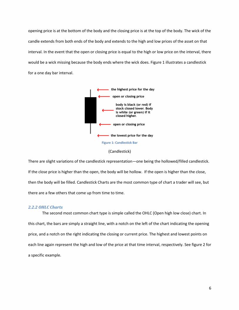
2.2.1 Candlestick Charts
Named for the shape of the bars, Candlestick charts display the price information using bars that
contain two parts, the body and the wick. The body of the candlestick is the central, wider part of the
bar which shows the open and closing prices of the bar. If the candlestick is red or black (depending on
the chart makers preference) then the bottom of the body is the closing price and the top is the opening
price, meaning the asset price decreased over the bar interval. If the candlestick is green then the
6
opening price is at the bottom of the body and the closing price is at the top of the body. The wick of the
candle extends from both ends of the body and extends to the high and low prices of the asset on that
interval. In the event that the open or closing price is equal to the high or low price on the interval, there
would be a wick missing because the body ends where the wick does. Figure 1 illustrates a candlestick
for a one day bar interval.
Figure 1: Candlestick Bar
(Candlestick)
There are slight variations of the candlestick representation—one being the hollowed/filled candlestick.
If the close price is higher than the open, the body will be hollow. If the open is higher than the close,
then the body will be filled. Candlestick Charts are the most common type of chart a trader will see, but
there are a few others that come up from time to time.
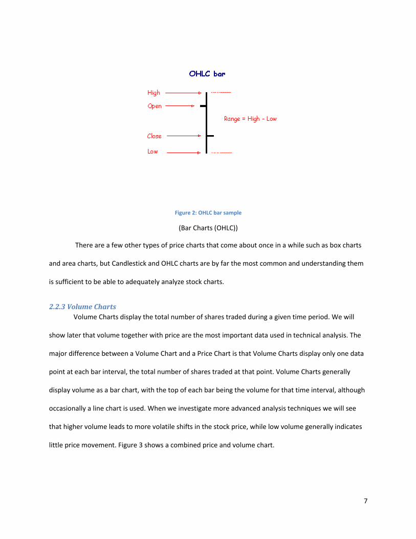
2.2.2 OHLC Charts
The second most common chart type is simple called the OHLC (Open high low close) chart. In
this chart, the bars are simply a straight line, with a notch on the left of the chart indicating the opening
price, and a notch on the right indicating the closing or current price. The highest and lowest points on
each line again represent the high and low of the price at that time interval, respectively. See figure 2 for
a specific example.
7
Figure 2: OHLC bar sample
(Bar Charts (OHLC))
There are a few other types of price charts that come about once in a while such as box charts
and area charts, but Candlestick and OHLC charts are by far the most common and understanding them
is sufficient to be able to adequately analyze stock charts.
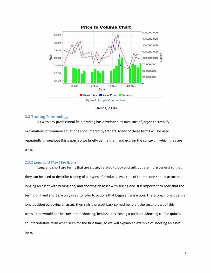
2.2.3 Volume Charts
Volume Charts display the total number of shares traded during a given time period. We will
show later that volume together with price are the most important data used in technical analysis. The
major difference between a Volume Chart and a Price Chart is that Volume Charts display only one data
point at each bar interval, the total number of shares traded at that point. Volume Charts generally
display volume as a bar chart, with the top of each bar being the volume for that time interval, although
occasionally a line chart is used. When we investigate more advanced analysis techniques we will see
that higher volume leads to more volatile shifts in the stock price, while low volume generally indicates
little price movement. Figure 3 shows a combined price and volume chart.
8
Figure 3: Sample Volume chart
(Haines, 2004)
2.3 Trading Terminology
As with any professional field, trading has developed its own sort of jargon to simplify
explanations of common situations encountered by traders. Many of these terms will be used
repeatedly throughout this paper, so we briefly define them and explain the context in which they are
used.
2.3.1 Long and Short Positions
Long and short are terms that are closely related to buy and sell, but are more general so that
they can be used to describe trading of all types of products. As a rule of thumb, one should associate
longing an asset with buying one, and shorting an asset with selling one. It is important to note that the
terms long and short are only used to refer to actions that begin a transaction. Therefore, if one opens a
long position by buying an asset, then sells the asset back sometime later; the second part of this
transaction would not be considered shorting, because it is closing a position. Shorting can be quite a
counterintuitive term when seen for the first time, so we will explain an example of shorting an asset
here.

9
Suppose we have been watching Apple’s stock price for a while, and have come to the
conclusion that the price is going to drop in the near future. To trade according to this theory we would
open a short position, meaning we would sell shares of Apple’s stock which we don’t own yet, but we
offer the promise to buy them back at a future date. This way, we are able to sell the stock while its
price is high, and buy it back to cover our debt when the price drops in the near future. The common
saying in trading that even those who have not ever studied financial markets is to “buy low and sell
high,” but shorting is another way to profit (in the opposite order) by selling high and buying low.
These definitions become slightly more complicated when dealing with options or futures
contracts, but one must keep in mind the association between long and buy and short and sell. To long
an option always means to purchase the option, making the person who opens the long position the
holder of the option. It is easy to be confused when dealing with put options where the person who
opens the long position actually has the option of selling the asset but it is still a long position because
the holder bought the option in the first place. Likewise, the person who writes the options (sells them)
is taking a short position in the transaction.
2.3.2 Bulls, Bears, Pigs, and Chickens
Bull, Bear, Pig, and Chicken are four terms that can be used to describe the trend of a market, or
a traders trading style. A bullish market is one that is trending upward, meaning the price is increasing.
Therefore, a bullish trader is a person who thinks the market is going to improve so he will open long
positions in the hopes of being able to sell his assets back when the rice goes up. A bearish market is the
opposite of a bullish one, so the price trend is downward and the bearish traders are opening short
positions. Bull and Bear refers to the trend or a trader’s perception of the future trend of a market,
while Pig and Chicken styles refer to the approach a trader takes after deciding on the market trend.

10
Chickens are traders that can be either bullish or bearish, but they are very cautious so they only
open positions when they are extremely confident about the direction of an asset, and even then they
will close a position shortly after opening it. Chickens will make marginal profits, but never risk losing a
large amount of money. Pigs on the other hand are reckless traders that open positions on the slightest
notion that the asset price is headed in a certain directions. Pigs are greedy traders who will hold their
positions for a long time so they can make big profits off of their investment. Accompanied with the
occasional large profit also comes the risk of large losses, because when a stock price is moving the
opposite direction that the Pig bet, they will wait longer to see if the price turns around, which often
leads to greater losses.
2.3.3 Overbought and Oversold Levels
Often an asset is referred to as overbought or oversold, depending on its current price. An
overbought asset is one which is at a very high price relative to its historical prices, so it is thought to
return to a more normal price level in the near future. The reason the term overbought is used is
because when a lot of people are buying an asset it increases the price of that stock or currency, so
when the price is very high it means that many people have bought the asset driving it out of its usual
price range, making it overbought. An oversold asset is one which has been sold excessively, driving its
price well below a normal level. Overbought and oversold levels are an essential tool in technical
analysis.
Closely related to the concept of overbought and oversold levels are support and resistance
levels. The support level for an asset is a low price that the asset will likely not go below, so when the
asset does approach or even go beyond the support level, it is thought that the assets prior history will
support the asset back to a usual price. Similarly, resistance levels are the unofficial upper bound on the
price such that when price levels above it are reached, they will resist further increases and tend back
11
down into the usual trading price range. As with overbought and oversold levels, the trouble with using
support and resistance is defining exactly where they are.
2.4 Markets
2.4.1 Foreign Exchange Market
We have already described what Forex trading is, but now we will go into more detail on the
specific details regarding the market in which currencies are traded.
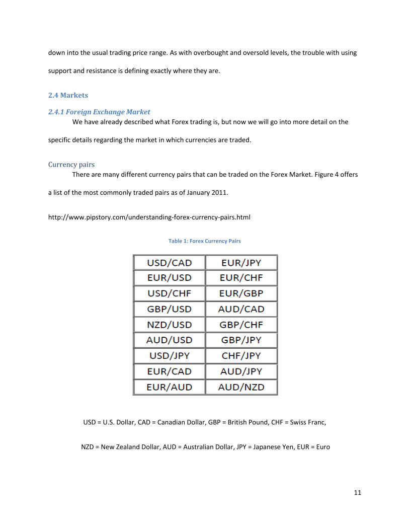
Currency pairs
There are many different currency pairs that can be traded on the Forex Market. Figure 4 offers
a list of the most commonly traded pairs as of January 2011.
http://www.pipstory.com/understanding-forex-currency-pairs.html
Table 1: Forex Currency Pairs
USD = U.S. Dollar, CAD = Canadian Dollar, GBP = British Pound, CHF = Swiss Franc,
NZD = New Zealand Dollar, AUD = Australian Dollar, JPY = Japanese Yen, EUR = Euro
12
Different currency pairs will vary in volatility, trend directions, trend times, and many other
aspects. One important variable in trading different currency pairs is the activity time for each pair.
Trading Times
A major upside to the Forex Market is that it is active 24 hours a day during the business week,
while stock exchanges have limited hours. While the market is constantly trading, there are hours that
are more active than others. The main trading times for the Forex market occur during the hours in
which the major stock exchanges (New York, London, and Tokyo) are open. During these hours, the
most trading goes on so the currency pairs are most volatile. Volatility is generally associated with the
most opportunity to make a profit (despite the highest risk), so these hours are continuously the most
active for the market.
Leveraging
Leveraging is a technique used in trading to obtain large profits with a minimal initial
investment. The Foreign Exchange Market boasts perhaps the highest achievable leverage of any
market. The means by which an investor can receive this leverage is by opening a Margin Account with a
broker. With a margin account, the investor is loaned money by the broker to invest in securities and
keep the marginal difference gained from each trade. Essentially, margin accounts magnify the profit or
losses incurred in the investor’s trades giving the possibility of greater returns and more severe losses. In
the Forex market, margin accounts generally offer 50:1, 100:1, or 200:1 leveraging. This means that
profits and losses could be multiplied up to 200 times what they would be if the investor had no
leveraging.
2.4. 2 Stock Exchange Markets
There are many stock exchanges throughout the world, but we will focus on the two large
American markets which are surprisingly different in the way they operate.
13
The New York Stock Exchange (NYSE)
The world’s largest stock exchange, the NYSE hosts most of the largest American businesses. The
NYSE is frequently depicted in media as a crowded room of businessmen screaming prices and
frantically trading stocks. There is some truth in this depiction because the NYSE is an Auction market,
meaning that all stocks are auctioned in a way such that participants offer prices they are willing to buy
or sell at until a compromise is reached. Until recently all trades going through the NYSE had to be called
in to someone on the floor of the exchange and executed by that person. Recently however the NYSE
has digitalized the trading process so that those outside of the market can exchange stocks immediately.
The downside to trading electronically versus having a seat in the exchange is that those who trade
electronically are charged a fee while those on the floor of the Exchange do not have to pay any such
fees. While this benefit is appealing, there are only 1366 seats available on the floor and they generally
cost about a million dollars to obtain.
The NASDAQ Stock Market
Unlike the NYSE, the NASDAQ is not tied to a room where humans trade stocks, it is completely
automated. The NASDAQ market relies on Market makers who deal stocks to buyers and sellers, while
on the NYSE buyers and sellers typically are trading with each other. Instead of orders being sent to an
auction floor, the NASDAQ has a network of computers that connects its users to market makers
instantly for trades. The NASDAQ was originally significantly smaller than the NYSE, but recently major
technology companies such as Microsoft and YAHOO! have boosted the size of the exchange.
2.5 Automated Trading
As a relatively recent technological upgrade to the trading industry, automated trading
strategies are still highly controversial even among experts. We hope to shed some light upon this
controversy by discussing both the positive and negative aspects to mechanical trading systems.

14
2.5.1 Benefits
To summarize the benefits of automated trading, one could say that computers can consistently
do things that humans can’t. Removing the human element to trading certainly also has many cons, but
here we will look at the positive aspects of it.
Instant Trading
Computers can boast reaction times that humans can’t physically hope to replicate. This
advantage can be critical in trading because often times a signal is generated in a security that triggers
everyone watching the security to invest in, and the ones who invest quickest will enjoy the most profit,
so in this case a computer’s response time could greatly improve profits.
Consistency
While humans make mistakes and can be forgetful, computers are not. While watching an asset
price move one might mistakenly forget a certain signal generally leads to a price movement in a certain
direction, and bet against that movement, costing the trader a lot of money. A computerized trading
system will never have this issue because it simply does everything you tell it to do, exactly that way,
every time it is executed. This way the user never has to worry about a human computational error or
lapse of memory. Eliminating this kind of mistake makes it easier to diagnose problems when losing
trades are made.
Emotionless
A major problem encountered by all traders is the inability to make difficult decisions without
the trader’s emotions becoming a factor. The most obvious winning trade could be available to a trader,
but if it involves the investment of a large percentage of their account, they may back out of the trade
just because they’re too concerned about what would happen if the trade doesn’t work out. Likewise,
being greedy and trying to get even bigger profits can cause a trader to hold a winning position for too
long until it becomes a losing one. Automated trading systems eliminate this problem because they are
completely emotionless, so they simply make the rational decision every time they trade.

15
Constant market monitoring
While humans watching the markets have limited attention spans and ability to observe what is
going on at all times, computers do not. A computer can watch an almost unlimited number of charts,
and it never has to take a break. This is especially critical when it comes to Forex trading where the
hours of operation can be difficult for a person to work through consistently, due to the time differences
in different parts of the world. As a result computer trading systems have an advantage over humans in
their increased capacity for watching markets.
2.5.2 Cons
As we have discussed, removing the human element from trading can lead to many benefits, but
not having a person making the decisions about when to trade can be harmful as well. Here we will
discuss several downfalls to automated trading systems and consider ways in which they can be
overcome.
Lack of Human Intuition
The primary fear in using a computerized system is the fact that it is impossible to write a
program that can perfectly simulate human logic. As a result, many are often concerned that automated
trading systems will make trades that a human would certainly be able to identify as losing, but they
somehow made it through the computers approval system so it made the trade anyways. This is a valid
concern as it is true that a computer program can only do as much as its writer tells it to, but with
enough bug testing this can be overcome. Programming languages today, particularly Tradestation’s
Easylanguage, offer coders the ability to tell a program to make just about every decision a human can
make. Therefore, with enough testing, it should be possible to write out in an automated trading
strategy every logical decision a human would make before opening a trade, so that there is no concern
about illogical trading.

16
Difficulty
A second limiting factor in the advancement of automated trading strategies is the difficulty of
writing such programs. It is uncommon enough to find a person with the appropriate skillset to be able
to profitably trade equities, but even more uncommon to find among that small group a person who is
familiar with computer programming. As a result, the advancement of automated trading systems has
been relatively slow, although as the computer science field grows in size we expect to see the number
of traders with coding experience to grow as well. As the field becomes more populated, it is likely that
the programming languages for trading will become more powerful and easier to use, so automated
trading systems will become much more effective and common.
Limited News Access
As we will go on to discuss, news announcements play a major role in any financial market. Any
news regarding a company or country or commodity can and usually will cause a major increase or
decrease in the price of the corresponding asset, depending on whether the news is good or bad.
Traders worry that automated trading systems can’t interpret news announcements and decide if they
are good or bad, so the system will possibly suffer major losses due to not understanding trends that
result from news. While there is no easy solution to this problem yet, some trading platforms such as
Tradestation offer the ability to check within a computer trading strategy when news announcements
are made. Therefore, it is possible to detect news announcements and halt actions performed by the
system for a reasonable amount of time after the announcement is made. This approach isn’t perfect
because if the system currently has an open position and a news announcement sends an asset price the
opposite direction, the strategy will still suffer a major loss. That being said, it is not much easier for a
person to predict when news announcements will be and how they will affect asset prices, so this
problem is shared among human and computer traders. It should be noted though that some news
announcements, such as the release of a countries monthly unemployment data, can be predicted so a
17
program could be written to avoid having positions open both before and after the news
announcement.
2.6 Systems Trading
2.6.1 Why are systems necessary?
No market goes up forever. The buy and hold strategy popular in the U.S. today is based on a
statistical anomaly. The U.S. and U.K. markets are the only countries in the world who have not had
markets completely disappeared at one point in time (Burnham, 2005). This has caused a misleading
assumption that markets in general will continue to rise.
However, technical and fundamental methods alone are not profitable either, often depending
on the market circumstances of the time. The greatest misconception by traders and investors is that
the market has a "magic formula" that can predict the market. Money is made on the use of well-
controlled entries and exits, especially those designed with to limit the loss that can occur. A systems
approach to trading can aid the trader or investor in controlling the timing of such entries and exits.
2.6.2 Discretionary versus Non-discretionary Systems
Systems are either discretionary, non-discretionary, or a combination of both. In discretionary
systems, intuition decides the entries and exits. Non-discretionary systems are those whose entries and
exits are determined mechanically by a set of formulas or rules.
Many exceptionally talented traders often use the discretionary approach, taking advantage of
their unique intuition and perception of the market. Looking for the "home run" this type of trader or
investor is likely to be more of the fearless romantic archetype: Exhibiting courage and skill with style
and resourcefulness under pressure not unlike The Three Musketeers. However, most traders do not
have the fortitude of mind, knowledge, and intuition to continue trading like this, often going broke or
"burning out."
18
On the other hand, the non-discretionary trader or investor is often a calm, calculating
individual. The majority of successful traders and investors use non-discretionary systems (Etzkorn
interview of Babcock, 1996). Usually engineers or of like mind, these individuals have studied the
markets, the various methods and indicators, and tested the systems through statistical analysis and
retrospective testing. Realizing that the market is imperfect and that history does not precisely repeat
itself, the non-discretionary individual designs and tests a system that minimizes risk and maximizes
return.
2.6.3 Composition of a system
A system is composed of rules. The rules can be simple such as "buy when the moving average
crosses above this line." However, rules can easily become more complicated such as "buy when moving
average A crosses above moving average B but oscillator C is between values D and E." Systems are
made of up rules which in turn are comprised of variables, the quantities used in rules, and parameters,
the actual values used in variables (Kirkpatrick and Dahlquist, 2007).
Pros and Cons of Non-discretionary Systems
The most important aspect of a non-discretionary system is the lack of emotion involved in the
actual trading. Traders and investors often fall prey to emotions leading to trading pitfalls--overtrading,
premature action, no action, and constant decision making (Kirkpatrick and Dahlquist, 2007). Properly
designed mechanical systems prevent large losses and risk of ruin. By providing strict risk control, the
system provides the trader or investor with certainty, confidence, and less stress. Anxiety, which stems
from uncertainty, is drastically reduced as the system can help structure how to read and understand,
and then react, to outcomes in the market.
Mechanical systems often make profits in clumps. The system will then often lose small
amounts of capital biding its time for the next "big clump." A loss of confidence in the system can result

19
in the premature modification of rules or abandonment of a system all-together right before it is about
to kick in. Therefore, considerable discipline is required in the creation and implementation of a system
including adhering to carefully outlined testing protocols.
2.6.4 How to Design a Nondiscretionary System
Requirements
• Understand what a discretionary or nondiscretionary system will do—be realistically knowledgeable,
and lean toward a nondiscretionary, mechanical system that can be quantified precisely and for which
rules are explicit and constant.
• Do not have an opinion of the market. Profits are made from reacting to the market, not by anticipating
it. Without a known structure, the markets cannot be predicted. A mechanical system will react, not
predict.
• Realize that losses will occur—keep them small and infrequent.
• Realize that profits will not necessarily occur constantly or consistently.
• Realize that your emotions will tug at your mind and encourage changing or fiddling with the system.
Such emotions must be controlled.
• Be organized—winging it will not work.
• Develop a plan consistent with one's time available and investment horizon—daily, weekly, monthly,
and yearly.
• Test, test, and test again, without curve-fitting. Most systems fail because they have not been tested or
have been over-fitted.
• Follow the final tested plan without exception—discipline, discipline, discipline. No one is smarter than
the computer, regardless of how painful losses may be, and how wide spreads between price and stops
may affect one's staying power.
(Kirkpatrick and Dahlquist, 2007)
Redefining Risk
A 50% loss will take a 100% return in order to break even. Likewise, a 100% gain can be brought
back by a 50% loss. Thus, it is important to understand that larger losses can require even larger gains to
be offset. Understanding risk is critical to trading and investing. While there are many definitions from
the world of academia in the world of financial markets risk is one thing. "How much capital am I going
to lose?" The amount of capital lost, or potentially lost is referred to as "drawdown." Drawdown is the
amount of decline in an equity from a peak. Drawdowns can occur, and often do, during entries and
exits.
20
Structure of the System
There are five critical steps in the initial design of a system: Philosophy and Logic; Market; Time-
horizon; Risk-control; and time-routine.
First, before putting the parts of a system together, it is important that the trader understands
how all rules implemented come together in the overall grand scheme of the system. The trader must
know why the methods chosen are the ones being used and what it conveys to the system. It is equally
crucial that the trader understands himself or herself and their various levels of comfort in making
trades.
Second, it is critical to identify the market the system is to target. Determining the market will
help the trader further consider the volatility and liquidity of the market and what it is specifically that
the system will be trading.
Third, a trader must analyze the time-horizon for the system. It is crucial that the trader
classifies his system in order to decide the appropriate time-horizon. For example, in trend-following
systems: longer periods; pattern systems: hours or days. This classification will further allow the trader
to decide what primary trades his system will perform such as swing trading or long-term investment.
Equally important is the time the trader has available to monitor his system. Whether the trader or
investor has all day or a few brief hours a week is something to be considered in the design of the
system.
Fourth is risk. Utilizing protective and trailing stops, price targets, and adjustments for volatility
and market state is critical in minimizing losses and preventing emotional swings from large and sudden
losses. A rule of thumb often followed by traders is a maximum risk of 2% of capital per trade.
Finally, establish a time routine involving the maintenance of the system. This encompasses
updating the system to account for changing market conditions, new trades, different entry points for
21
new trades and exits points for both existing and new trades. Along with system administration, keep a
trading plan, journal, and daily equity chart.
Types of Systems
Trend Following
Instead of following the buy-low sell-high philosophy, trend following is a buy-high sell-higher
system. Due to larger moves and fewer transactions, and transaction costs, the trend following system is
often the non-discretionary system of choice for hedge funds and commodity traders. By acting as soon
as a trend has been reliably identified, this system ignores the peaks and valleys that occur throughout
the time-horizon trading the directional trend. However trend following is prone to a stagnation in
performance during a "trading range" market.
Moving Average
Moving averages are simple systems that calculate a dynamic average over a given time span. It
is important to note that while two moving averages have shown to be more successful than one
moving average, systems that implement three or more are often weaker due to the more complex
rules involved.
Breakout
A variation of the moving average, the breakout system implements channels or bands, which
use moving averages. When the price action moves outside the aforementioned indicators, the system
will signal a buy or sell. Breakout systems usually include a volatility indicator as well.
Pattern Recognition
Pattern recognition systems can be divided into two subcategories: large scale and small, or
short, pattern systems. Pattern systems require considerable testing due to the sheer amount of
variables and their respective influences in a given market. Large patterns are generally less compatible
to computer recognition due to the ambiguity involved in correctly indentifying the beginning and end
of a given pattern. Short pattern systems are designed to quickly identify fast movements that
22
potentially indicate upcoming extreme movements. Due to the slow nature of moving averages, short
patterns provide an advantage in that they provide indications or warnings of potential changes that
would be lost on longer term data systems.
Pattern recognition systems are not ideal for pure mechanical systems. These systems are often
better used in conjunction with trader experience and intuition to aid the trader in his or her decisions.
It is also interesting to note that despite the vast advances in computing technology, the human brain
outperforms computers in recognizing patterns (Feng, 2007).
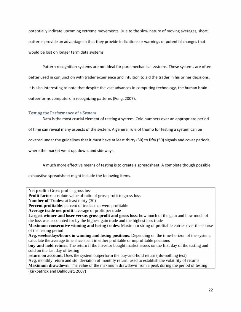
Testing the Performance of a System
Data is the most crucial element of testing a system. Cold numbers over an appropriate period
of time can reveal many aspects of the system. A general rule of thumb for testing a system can be
covered under the guidelines that it must have at least thirty (30) to fifty (50) signals and cover periods
where the market went up, down, and sideways.
A much more effective means of testing is to create a spreadsheet. A complete though possible
exhaustive spreadsheet might include the following items.
Net profit : Gross profit - gross loss
Profit factor: absolute value of ratio of gross profit to gross loss
Number of Trades: at least thirty (30)
Percent profitable: percent of trades that were profitable
Average trade net profit: average of profit per trade
Largest winner and loser versus gross profit and gross loss: how much of the gain and how much of
the loss was accounted for by the highest gain trade and the highest loss trade
Maximum consecutive winning and losing trades: Maximum string of profitable entries over the course
of the testing period
Avg. weeks/days/hours in winning and losing positions: Depending on the time-horizon of the system,
calculate the average time slice spent in either profitable or unprofitable positions
buy-and-hold return: The return if the investor bought market issues on the first day of the testing and
sold on the last day of testing
return on account: Does the system outperform the buy-and-hold return ( do-nothing test)
Avg. monthly return and std. deviation of monthly return: used to establish the volatility of returns
Maximum drawdown: The value of the maximum drawdown from a peak during the period of testing
(Kirkpatrick and Dahlquist, 2007)
23
2.7 Fundamental Analysis
As we have discussed, there is a general (not exact) correlation between how profitable a
country or company is and the value per unit of that entities currency or stock. A common question
among financial analysts is how one can determine exactly how well a country or company is
performing. Due to the complex nature of global economies and large corporations there are many
different theories on the best approach to answer this question, and over time the approaches have
become increasingly intricate. The approaches for Forex and Stocks vary greatly so we will look at each
independently.
2.7.1 Stocks
Since the Sarbanes-Oxley Act of 2002 was passed, corporations have been required to keep
extremely accurate records of their financial performance available to the public. These records serve as
the basis for a great deal of financial analysis done on companies. There are three primary documents
that all corporations publish and are used for gauging a company’s profitability; they are the Balance
Sheet, Income Statement, and Cash Flow Statement. We will look at ways the first two statements are
used in determining when to invest.
Balance Sheet
The balance sheet is recorded at the end of every month and is generally described as a
snapshot of a company’s financial status at the instant it was released. The balance sheet follows the
equation Assets = Liabilities + Owner’s Equity, where a few examples of items in each category are listed
below.
Assets
Current assets
1. Cash and cash equivalents 2. Inventories 3. Accounts receivable Non-current assets (Fixed assets)
24
1. Property, plant and equipment 2. Investment property, such as real estate held for investment purposes 3. Intangible assets
Liabilities
1. Accounts payable 2. Financial liabilities, such as promissory notes and corporate bonds 3. Liabilities and assets for current tax
Equity
1. Issued capital and reserves attributable to equity holders of the parent company (controlling interest)
2. Non-controlling interest in equity
Equity is perhaps the hardest of the three to understand, but one can just think of it as funds the
company owes to its shareholders.
The question of how a balance sheet can be used to determine if a company is a good
investment is a valid one that remains unanswered. As has been stated a balance sheet provides a view
of how the company is doing at a certain point in time, so if other factors lead an investor to believe that
a certain stock is worth buying, that investor can look at the company balance sheet to see how the
company is doing in terms of cash and debt at that time. It is common to compare current balance sheet
values with those of previous business periods to see how the company is doing relative to its previous
record. For example, if a company’s balance sheet shows its cash value is half of what it was a year ago
and its debt is twice what it was a year ago, one can conclude that that company is probably not doing
well so buying their stock would be a bad idea. Many values and ratios are calculated using values found
on the balance sheet and income statement that are used to quantify different factors affecting how
good of an investment a company is. We will study these figures after a quick summary of the income
statement.
25
Income Statement
While the balance sheet shows how a company stands at an instant in time, the income
statement displays how the company performed over its last business period. The equation summarizing
the income statement is Net Income = Revenue – Expenses. Income Statements then become
interesting to investors because they show exactly how profitable a company was over the last period.
Again a common practice would be to compare the net income of the most recent period to that of
previous periods to see if the companies business is growing or shrinking. A company whose net income
has shrank every period for the past five periods is a prime example of an investment that an income
statement would ward one away from. While interpreting things directly from financial statements can
be useful, there are many more ways we can use the information in the financial statements to help us
invest.
Financial Ratios
Financial ratios are values derived from commonly available company data that determine the
profitability of an investment. These ratios fall into three categories, liquidity, solvency, and profitability.
Liquidity
Liquidity refers to how much of a company’s assets could be sold without suffering a major loss
in value. Cash is an example of a perfectly liquid asset since there is no conversion required to have it
turned to currency, while inventory must be sold in order to be turned into cash. The reason investors
care about liquidity is that it tells us a business’s ability to meet its financial obligations. If a company
lacks liquidity, investors should be worried that the company may have debt issues in the near future
which would reduce the company’s stock value.
We have two common measures for calculating the liquidity of a company; they are the Current
Ratio and the Current Cash Debt Coverage Ratio(CCDCR). The formulas for the two ratios are given by
equations 1 and 2.
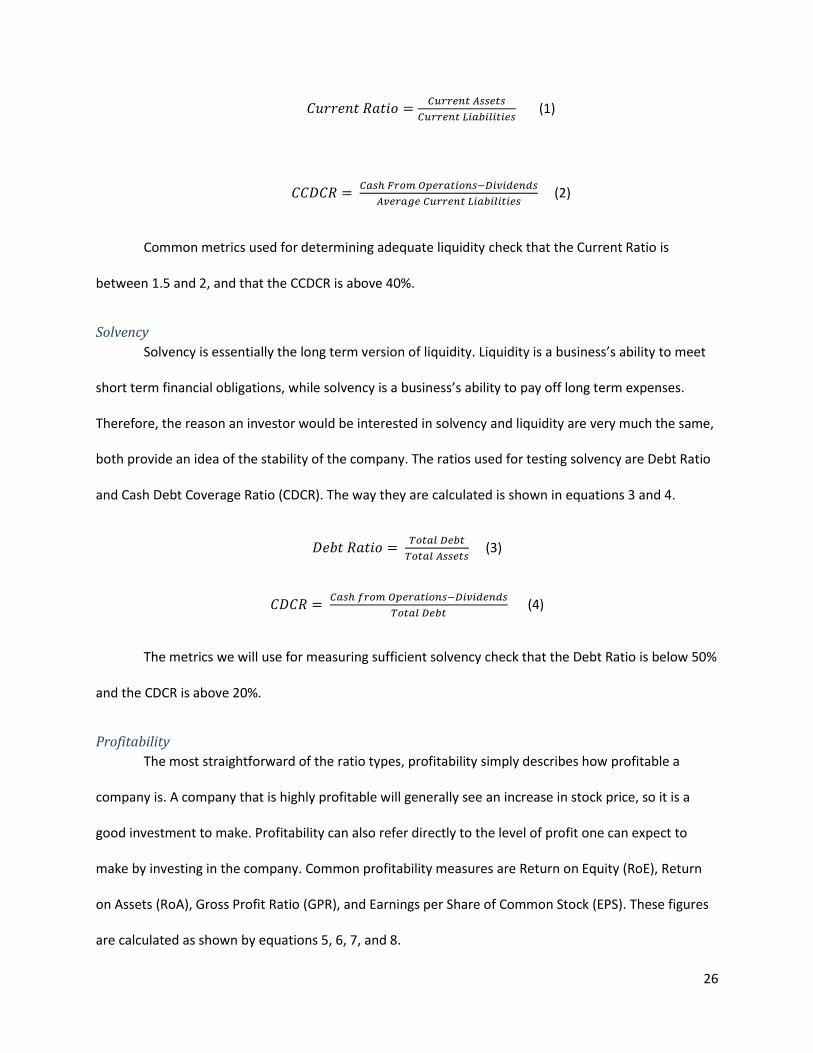
26
(1)
(2)
Common metrics used for determining adequate liquidity check that the Current Ratio is
between 1.5 and 2, and that the CCDCR is above 40%.
Solvency
Solvency is essentially the long term version of liquidity. Liquidity is a business’s ability to meet
short term financial obligations, while solvency is a business’s ability to pay off long term expenses.
Therefore, the reason an investor would be interested in solvency and liquidity are very much the same,
both provide an idea of the stability of the company. The ratios used for testing solvency are Debt Ratio
and Cash Debt Coverage Ratio (CDCR). The way they are calculated is shown in equations 3 and 4.
(3)
(4)
The metrics we will use for measuring sufficient solvency check that the Debt Ratio is below 50%
and the CDCR is above 20%.
Profitability
The most straightforward of the ratio types, profitability simply describes how profitable a
company is. A company that is highly profitable will generally see an increase in stock price, so it is a
good investment to make. Profitability can also refer directly to the level of profit one can expect to
make by investing in the company. Common profitability measures are Return on Equity (RoE), Return
on Assets (RoA), Gross Profit Ratio (GPR), and Earnings per Share of Common Stock (EPS). These figures
are calculated as shown by equations 5, 6, 7, and 8.
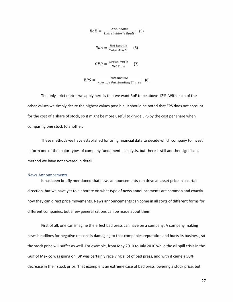
27
(5)
(6)
(7)
(8)
The only strict metric we apply here is that we want RoE to be above 12%. With each of the
other values we simply desire the highest values possible. It should be noted that EPS does not account
for the cost of a share of stock, so it might be more useful to divide EPS by the cost per share when
comparing one stock to another.
These methods we have established for using financial data to decide which company to invest
in form one of the major types of company fundamental analysis, but there is still another significant
method we have not covered in detail.
News Announcements
It has been briefly mentioned that news announcements can drive an asset price in a certain
direction, but we have yet to elaborate on what type of news announcements are common and exactly
how they can direct price movements. News announcements can come in all sorts of different forms for
different companies, but a few generalizations can be made about them.
First of all, one can imagine the effect bad press can have on a company. A company making
news headlines for negative reasons is damaging to that companies reputation and hurts its business, so
the stock price will suffer as well. For example, from May 2010 to July 2010 while the oil spill crisis in the
Gulf of Mexico was going on, BP was certainly receiving a lot of bad press, and with it came a 50%
decrease in their stock price. That example is an extreme case of bad press lowering a stock price, but

28
less drastic versions of that happen every day. An investor who is holding shares of a company should be
mindful of these news announcements so they can sell their shares immediately should a negative
announcement come.
News announcements aren’t always a bad thing though; they can work in the positive direction
as well. Apple has been performing extremely well on the Market as of late and a lot of their success is
attributed to the frequency with which they release new products. With each new product release
comes a news announcement that is interpreted as a positive sign for the company so the stock price
increases. Other types of positive news announcements could be a company announcing the acquisition
of another company, a major charitable donation, or the release of some sort of major business ranking
list that gives a certain company a high placement(like Fortune’s list of America’s Most Admired
Companies).
A common philosophy regarding trading stocks based on news announcements is described by
the statement “buy on the rumor, sell on the news.” What this saying means is that when good news is
speculated to come in the future, one should buy the stock, and as soon as the news is released, sell it.
The reasoning behind this is that in general traders will overhype a new development in the company,
and when the actual news about the new development comes out, it will be less impressive than what
they expected. An example of this would occur when a company is set to release a new product in a
month and speculators think the product will do extremely well so the stock price soars. This philosophy
predicts that when the news comes out about how many units were actually sold in the new product’s
first day(s) on the market, the numbers will be underwhelming and the stock price will drop. The
interesting thing about this philosophy is that it has even held true in cases where product sales set
world records, just because speculation before the news release can get so out of hand. “Buy on the
29
rumor, sell on the news” is a historically tested statement that has had plenty of success over time, but
as with any overly simplified trading strategy, it is also wrong quite frequently.
Another type of news announcement we can consider is a combination of a news
announcement and the financial data we discussed previously. Immediately upon the release of major
financial documents, stock prices will generally see a short term trend related to how the market
interprets the newly published data. If an income statement is released that shows net income that is
100% larger than that of the previous period, the stock will likely see an increase. Likewise a significant
decrease in net income published would cause an immediate decrease in stock price. News
announcements play a major role in the trading of stocks and understanding how they drive prices will
greatly enhance our ability to develop a profitable trading algorithm.
2.7.2 Foreign Exchange
Fundamental analysis takes a much different form when applied to Forex trading because of the
global scope of the trading, the difference between national economies and company profitability, and
the nature of paired currencies. There isn’t necessarily an exact counterpart to the financial statements
we used to analyze stocks for Forex, but there are a few common types of data we can gather for any
country.
National Economic Data
Just like the profitability of a company drives the price of its stock up, the success of a nation’s
economy brings up the value of its currency. Success of a countries economy can be somewhat harder to
define for this reason. A thriving economy would ideally feature a low national debt (or even a surplus)
and a large Gross Domestic Product (GDP), but the problem is that these two things have been inversely
related in the recent history. One would seek to find a balance between the two data points so that the
GDP is at a high level with a relatively low national debt. Regardless, these two economic statistics are

30
just a couple of many figures used to quantify the success of a national economy, so we will examine a
few other indicators to see if we can more easily calculate a successful national economy.
Perhaps the most common economic indicator next to GDP and national debt is the
unemployment rate in a country. When many people are unemployed, the economy is perceived as
struggling so its currency is weaker. The converse is also true that an economy with a low
unemployment rate is performing well. Another factor closely related to unemployment rate is average
duration of unemployment, which explains the amount of time the average unemployed person spends
looking for work. The longer the average person is looking for work, the worse the economy looks, and
vice versa.
The other major statistic used for looking at the strength of an economy is the countries interest
rate. When a country has a higher interest rate, its currency will perform well because investors will
want to deposit their money where they earn a higher interest rate. Lower interest rates drive investors
away from countries, weakening their currency. With Forex there is a link between these sorts of
statistics and a major group of news announcements that drive prices; both revolve around the
government.
Government Announcements
These statistics we have been discussing are all generally recorded by governments of the
countries, like the Bureau of Labor Statistics calculated unemployment data in the U.S. The government
can influence the strength of its currency through other means as well. One common example is through
the passing of new legislation. If a law is passed that favors business, the currency will generally grow
stronger, while laws restricting business will hurt the currency value. Similarly, when politicians are
elected that business thinks will help them, the economy booms and so does the currency value. This all
follows the philosophy outlined before that the value of a currency depends on perceived future
31
direction of the country’s economy. There are also several factors that are not government centric but
can still strongly influence a currency value.
Other Events
Often much harder to predict, major unexpected events can play a big part in effectively trading
currencies. One example that we have seen recently is the way in which a major natural disaster can
decimate a currency. In early March 2011 when major earthquakes struck Japan, its currency suffered a
significant decrease in value, although it did rebound quickly afterward. Similar to natural disaster
driven price movements are the trend in prices following acts of war.
A turbulent domestic situation might be the one factor most likely to scare off investors. No one
wants to invest their money in something that is very uncertain, so whenever there is a conflict in a
country its currency tends to suffer. A recent example was when Egyptian President Hosni Mubarak
refused to immediately step down, and the people of Egypt rioted. At that time the Egyptian pound hit
an extreme low value as many investors wanted to take their money out of Egyptian currency as quickly
as possible.
Major national events can be positive as well, helping strengthen a nation’s currency. The World
Cup certainly helped South Africa, whose currency has been growing in strength recently. Other major
events like the Olympics or a technological advancement will also tend to strengthen the currency of a
country. These events are often difficult to predict but are key to understand to effectively trade
currencies.
2.8 Technical Analysis
Technical analysis differs from fundamental analysis in that rather on focusing on features of a
company or country or things going on in the world, it instead looks only at the asset price data over
time. The time frame inspected can range from 2 hours to 100 years, and the way data is used also
varies greatly, leaving the possibility for a wide variety of technical analysis. Technical analysis is

32
generally a much bigger factor in the decision making process for day traders than fundamental analysis
is, so it is especially important for us to focus on as it will have a large role in our automated trading
systems.
2.8.1 Technical Indicators
It is impossible to talk about technical analysis of stock or currency price data without
mentioning technical indicators. The reason for this is that technical indicators essentially summarize all
technical analysis. A technical indicator is an equation calculated based on either price or volume data
(or both) in an effort to display a new type of information about the asset. The type of information
displayed varies greatly, as does the way a trader should interpret it, so we will look at a few
generalizations that can be made about indicators.
Type of Information Displayed
The first question one should ask when looking at an indicator chart is “What is this graph
showing me?” There are a few common answers to that question when dealing with technical
indicators, but they can be misleading too. The reason for that is that there are multiple indicators that
demonstrate the same type of information but in different ways. For example, many indicators show
overbought and oversold levels for an asset, but some of the indicators take on low values when the
asset is overbought, while others take on high values for overbought assets. One must be careful when
using indicators to properly interpret the data provided.
A few other common characteristics that appear in indicators are volatility, trend strength, and
volume. Volatility indicators usually take on high values when asset prices are fluctuating strongly, while
an asset whose price is not oscillating very much will have a low volatility and that usually means a low
value on the indicator. Trend strength indicators attempt to predict the magnitude of a trend that a
security is currently following. For example, if observing an equity that has had an increasing price for
the last few periods, a strong trend would continue increasing at a fast rate, while a weak one would

33
probably slow down or reverse direction shortly after. Volume indicators are similar to volatility ones,
because they show how frequently shares are being exchanged, and more shares that are being traded
means the price will move more. These types of information are the most frequently seen in technical
indicators, although others are possible. We will now look at the different ways in which indicators can
display this information.
Leading and Lagging Indicators
One way to classify indicators is whether they generate buy/sell signals, or simply support them.
This is the distinction one can draw between leading and lagging indicators, which either attempt to
predict trend data (leading), or reflect previous trends (lagging). The way leading indicators are used is
quite intuitive; they predict where the price is going to go, although not always right, so the investor
knows whether to long or short and asset. Lagging indicators tend to be slightly more confusing, but
after some consideration should make complete sense. Since lagging indicators tend to trail the pattern
of the market, they can confirm the strength of a trend. If an asset price starts dropping rapidly, one
can’t expect the price to stop decreasing until the lagging indicator has recovered. As a result lagging
indicators are a valuable tool in confirming long term trends in price changes for assets.
Oscillators
Oscillators are a type of indicator that fluctuate around a center point or between two boundary
points. These boundary points can be hard or soft limits, meaning that it may be mathematically
impossible to exceed them, or just extremely unlikely that a value will be found outside of the bounds.
Overbought/oversold oscillators are by far the most common type of oscillator. Oscillators can provide
buy and sell signal in many different ways, depending on the specific oscillator observed.
Crossovers
Crossover indicators are possibly the easiest kind of indicator to read. They simply require the
user to draw a horizontal line across the graph, and wait for the indicator line to cross over it. Some of
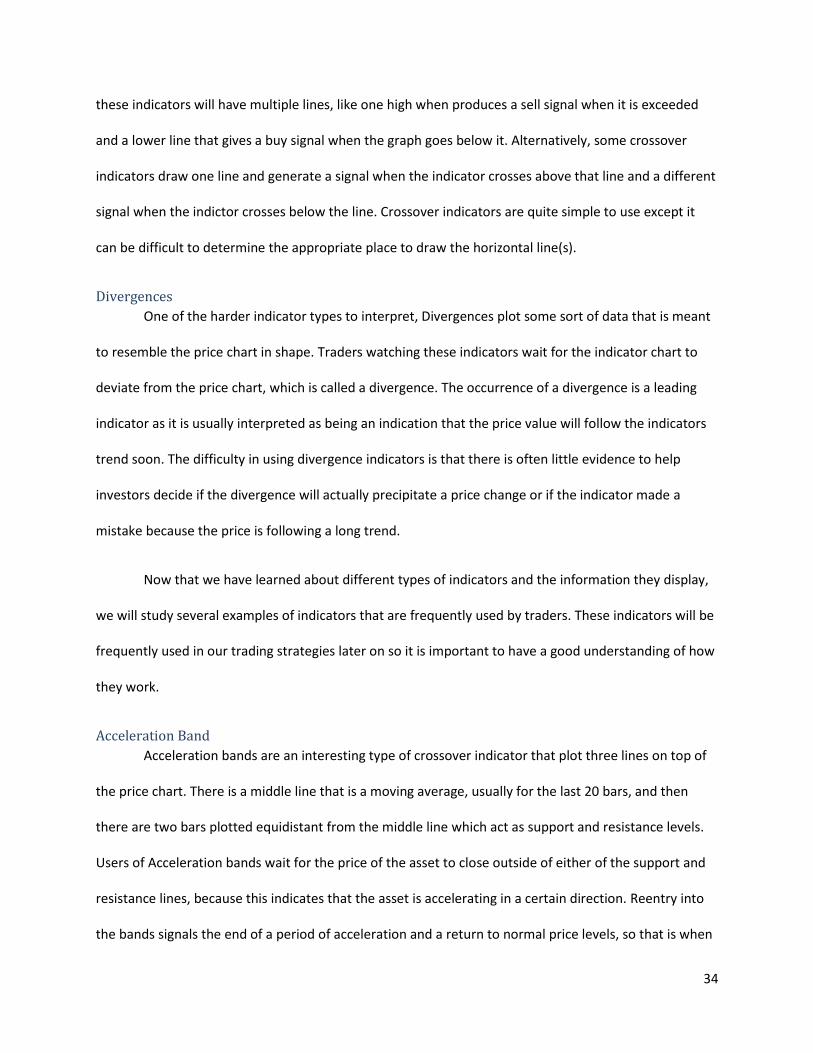
34
these indicators will have multiple lines, like one high when produces a sell signal when it is exceeded
and a lower line that gives a buy signal when the graph goes below it. Alternatively, some crossover
indicators draw one line and generate a signal when the indicator crosses above that line and a different
signal when the indictor crosses below the line. Crossover indicators are quite simple to use except it
can be difficult to determine the appropriate place to draw the horizontal line(s).
Divergences
One of the harder indicator types to interpret, Divergences plot some sort of data that is meant
to resemble the price chart in shape. Traders watching these indicators wait for the indicator chart to
deviate from the price chart, which is called a divergence. The occurrence of a divergence is a leading
indicator as it is usually interpreted as being an indication that the price value will follow the indicators
trend soon. The difficulty in using divergence indicators is that there is often little evidence to help
investors decide if the divergence will actually precipitate a price change or if the indicator made a
mistake because the price is following a long trend.
Now that we have learned about different types of indicators and the information they display,
we will study several examples of indicators that are frequently used by traders. These indicators will be
frequently used in our trading strategies later on so it is important to have a good understanding of how
they work.
Acceleration Band
Acceleration bands are an interesting type of crossover indicator that plot three lines on top of
the price chart. There is a middle line that is a moving average, usually for the last 20 bars, and then
there are two bars plotted equidistant from the middle line which act as support and resistance levels.
Users of Acceleration bands wait for the price of the asset to close outside of either of the support and
resistance lines, because this indicates that the asset is accelerating in a certain direction. Reentry into
the bands signals the end of a period of acceleration and a return to normal price levels, so that is when
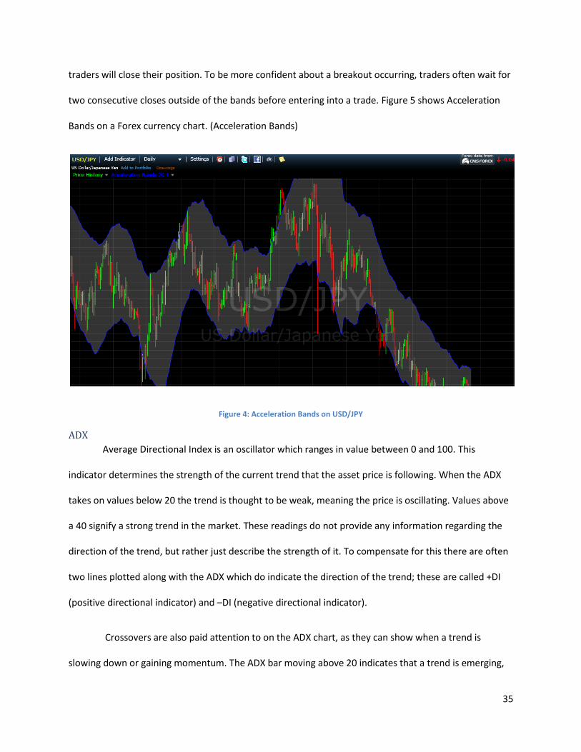
35
traders will close their position. To be more confident about a breakout occurring, traders often wait for
two consecutive closes outside of the bands before entering into a trade. Figure 5 shows Acceleration
Bands on a Forex currency chart. (Acceleration Bands)
Figure 4: Acceleration Bands on USD/JPY
ADX
Average Directional Index is an oscillator which ranges in value between 0 and 100. This
indicator determines the strength of the current trend that the asset price is following. When the ADX
takes on values below 20 the trend is thought to be weak, meaning the price is oscillating. Values above
a 40 signify a strong trend in the market. These readings do not provide any information regarding the
direction of the trend, but rather just describe the strength of it. To compensate for this there are often
two lines plotted along with the ADX which do indicate the direction of the trend; these are called +DI
(positive directional indicator) and –DI (negative directional indicator).
Crossovers are also paid attention to on the ADX chart, as they can show when a trend is
slowing down or gaining momentum. The ADX bar moving above 20 indicates that a trend is emerging,

36
while ADX crossing below 40 predicts the end of a trending period. Another type of crossover that is
looked at is when +DI and –DI intersect. +DI crossing above –DI indicates a bullish signal, while –DI
crossing above +DI is a bearish signal. Figure 6 displays a sample ADX. (Average Directional Index (ADX),
1999)
Figure 5: ADX Plotted below AAPL
Average True Range
The Average True Range (ATR) is a very simple indicator which determines the volatility of an
asset price over the last few bars. The true range of an asset is simply the high price minus the low price
for the current bar. As one might expect, the ATR is simply an average of the true ranges for a set
number of bars, generally the last 14. To smooth out the ATR, it is more common to see it be computed
as an average of each of the ATR values for the last 13 bars and the current true range. Doing this
reduces the effect that previous outliers will have on the computation, but if the current bar is an outlier

37
it will have a strong effect, which is a good thing because the most recent point most strongly describes
the current situation. See figure 7 for an example of ATR. (Average True Range)
Figure 6: ATR below AAPL
Stochastics
Stochastics is an oscillator based on comparing the current closing price to its price range over
the last X periods, which is done by finding what percentile of the overall range the closing price falls in.
The theory behind using this figure is that prices tend to close near critical points before turning points
because momentum tends to change direction before price does.
The name for this first number is %K, there is also a second calculation done to find %D, which is a 3
period moving average of %K. %D is meant to be used as a long term figure to compare with %K, the
short term figure.
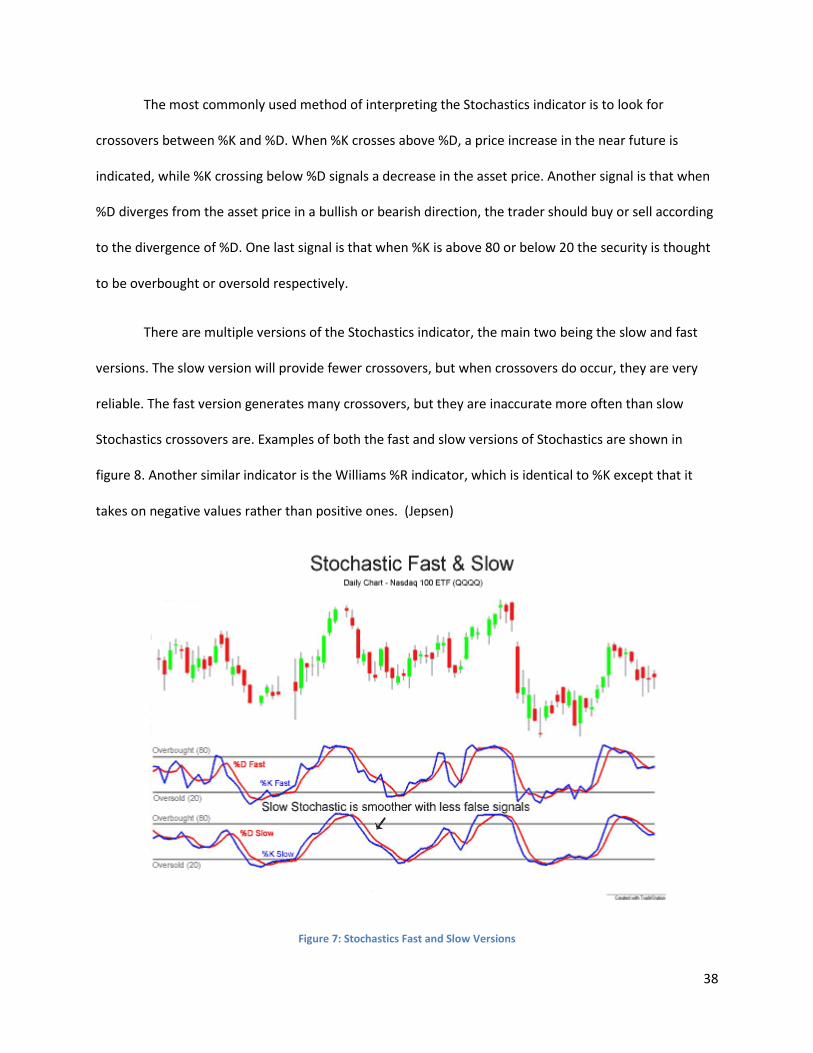
38
The most commonly used method of interpreting the Stochastics indicator is to look for
crossovers between %K and %D. When %K crosses above %D, a price increase in the near future is
indicated, while %K crossing below %D signals a decrease in the asset price. Another signal is that when
%D diverges from the asset price in a bullish or bearish direction, the trader should buy or sell according
to the divergence of %D. One last signal is that when %K is above 80 or below 20 the security is thought
to be overbought or oversold respectively.
There are multiple versions of the Stochastics indicator, the main two being the slow and fast
versions. The slow version will provide fewer crossovers, but when crossovers do occur, they are very
reliable. The fast version generates many crossovers, but they are inaccurate more often than slow
Stochastics crossovers are. Examples of both the fast and slow versions of Stochastics are shown in
figure 8. Another similar indicator is the Williams %R indicator, which is identical to %K except that it
takes on negative values rather than positive ones. (Jepsen)
Figure 7: Stochastics Fast and Slow Versions

39
Bollinger Bands
Bollinger Bands are very similar in usage to the Acceleration Bands indicator which was
discussed early. As with the Acceleration Bands, Bollinger Bands plot three lines around the price chart,
where there is a middle line, high line, and low line. The middle line is a simple moving average of the
price over the last N bars, and the high and low lines are computed by adding or subtracting a certain
number of standard deviations from the middle line. The way in which Bollinger Bands are used is
basically identical to the way we described using Acceleration Bands, so we will not go into detail about
it, but the general idea is again to look for the price to move outside of the high or low bands. An
example of Bollinger Bands is shown in figure 9. (Bollinger Bands)
Figure 8: Bollinger Bands plotted on the S&P 500 chart

40
Elliott Wave Oscillator
The Elliott Wave Oscillator is an indicator designed to be used for the purpose of applying
Elliott Wave Theory, which we will summarize briefly.
Two ideas are central to Elliott Wave theory; they are that every action is followed by a
reaction and that throughout time prices have frequently followed one pattern and will
continue to in time. The pattern is that the price will have five movements (waves) in the
direction of the trend it is following, and each movement is followed by a correcting wave that
takes the price back to its normal level. This process is clearly shown in figure 10 for an asset
following an upward trend.
Figure 9: Elliott Wave Theory predicted price movement
Further, the waves in the direction of the trend will have five waves within them, while
the correcting waves will only have three waves within them. The inside of the first type of
wave is shown in figure 10. (Elliot Wave Theory)

41
Figure 10: Intrawave Elliot Waves
Elder Ray Bear/Bull Power
Elder Ray Bull and Bear power are very closely related technical indicators that are used to
quantify the feeling of investors regarding a certain security. Bear power is the total bearish feelings of
investors about the security while bull power is the bullish feelings, so naturally the two are inversely
related. Bull Power is calculated by subtracting an exponential moving average (EMA) of closing prices
over N periods from the daily high price, while bear power subtracts the EMA from the daily low price.
The resulting figures provide a look at where the closing prices have been in relation to the high or low
price for that period, giving additional wait to the more recent closing prices so the indicators more
strongly reflect the current situation. When closing prices have been relatively high, bull power will be
low, maybe even negative, and bear power will be very negative.
In general a high value of bull power and bear power is a bullish sign, while both indicators
taking on low values is a bearish sign. Traders generate signs from these indicators in a few different
ways, generally not just by looking at the current values of the two. One method is to open a long
position if the most recent peak of bear power is higher than the previous peak, and bear power is
negative but rising. A signal to short occurs when latest bear power minimum is lower than the previous
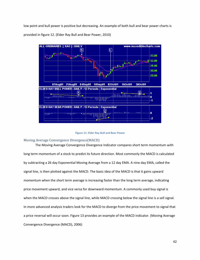
42
low point and bull power is positive but decreasing. An example of both bull and bear power charts is
provided in figure 12. (Elder Ray Bull and Bear Power, 2010)
Figure 11: Elder Ray Bull and Bear Power
Moving Average Convergence Divergence(MACD)
The Moving Average Convergence Divergence Indicator compares short term momentum with
long term momentum of a stock to predict its future direction. Most commonly the MACD is calculated
by subtracting a 26 day Exponential Moving Average from a 12 day EMA. A nine day EMA, called the
signal line, is then plotted against the MACD. The basic idea of the MACD is that it gains upward
momentum when the short term average is increasing faster than the long term average, indicating
price movement upward, and vice versa for downward momentum. A commonly used buy signal is
when the MACD crosses above the signal line, while MACD crossing below the signal line is a sell signal.
In more advanced analysis traders look for the MACD to diverge from the price movement to signal that
a price reversal will occur soon. Figure 13 provides an example of the MACD indicator. (Moving Average
Convergence Divergence (MACD), 2006)
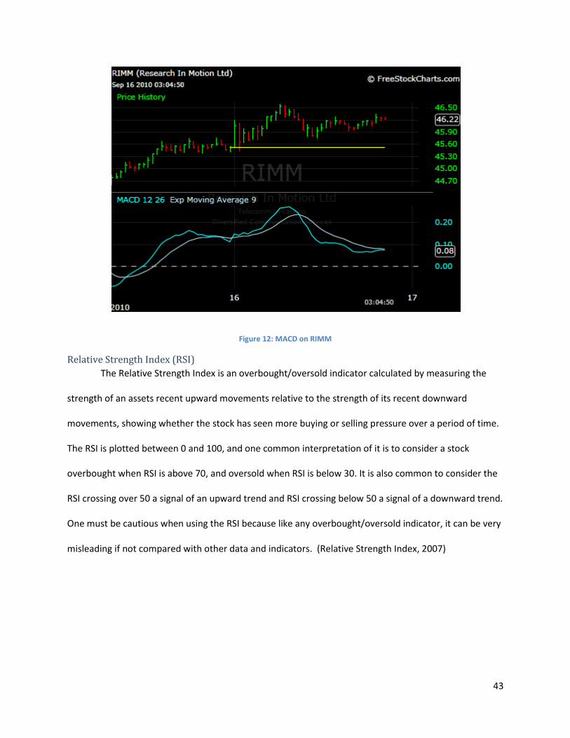
43
Figure 12: MACD on RIMM
Relative Strength Index (RSI)
The Relative Strength Index is an overbought/oversold indicator calculated by measuring the
strength of an assets recent upward movements relative to the strength of its recent downward
movements, showing whether the stock has seen more buying or selling pressure over a period of time.
The RSI is plotted between 0 and 100, and one common interpretation of it is to consider a stock
overbought when RSI is above 70, and oversold when RSI is below 30. It is also common to consider the
RSI crossing over 50 a signal of an upward trend and RSI crossing below 50 a signal of a downward trend.
One must be cautious when using the RSI because like any overbought/oversold indicator, it can be very
misleading if not compared with other data and indicators. (Relative Strength Index, 2007)
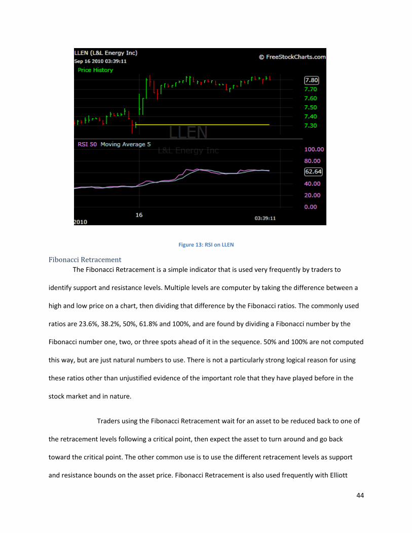
44
Figure 13: RSI on LLEN
Fibonacci Retracement
The Fibonacci Retracement is a simple indicator that is used very frequently by traders to
identify support and resistance levels. Multiple levels are computer by taking the difference between a
high and low price on a chart, then dividing that difference by the Fibonacci ratios. The commonly used
ratios are 23.6%, 38.2%, 50%, 61.8% and 100%, and are found by dividing a Fibonacci number by the
Fibonacci number one, two, or three spots ahead of it in the sequence. 50% and 100% are not computed
this way, but are just natural numbers to use. There is not a particularly strong logical reason for using
these ratios other than unjustified evidence of the important role that they have played before in the
stock market and in nature.
Traders using the Fibonacci Retracement wait for an asset to be reduced back to one of
the retracement levels following a critical point, then expect the asset to turn around and go back
toward the critical point. The other common use is to use the different retracement levels as support
and resistance bounds on the asset price. Fibonacci Retracement is also used frequently with Elliott

45
Wave Theory. Figure 15 illustrates Fibonacci Retracement levels being drawn for an asset. (Deaton,
2008)
Figure 14: Fibonacci Retracement
Ichimoku Cloud
The Ichimoku Cloud is made up of four components that are each computer based on historical
critical points. Three of the components, the Tenkan Sen, Kijun Sen, and the Senkou Span B are
computed by averaging the highest high and lowest low over the past 8, 22, and 44 periods,
respectively. The Senkou Span A is computed by averaging the Tenkan Sen and Kijun Sen, then plotting
the point 26 bars ahead of the current price action, and Senkou Span B is plotted 22 bars ahead. The
cloud is considered the area in between the two Senkou Spans, and creates support and resistance
levels for the asset price. It is also common to see a fifth component, the Chikou Span, which the closing
price from 26 periods ago.
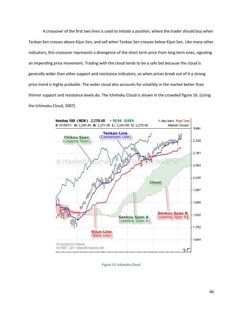
46
A crossover of the first two lines is used to initiate a position, where the trader should buy when
Tenkan Sen crosses above Kijun Sen, and sell when Tenkan Sen crosses below Kijun Sen. Like many other
indicators, this crossover represents a divergence of the short term price from long term ones, signaling
an impending price movement. Trading with the cloud tends to be a safe bet because the cloud is
generally wider than other support and resistance indicators, so when prices break out of it a strong
price trend is highly probable. The wider cloud also accounts for volatility in the market better than
thinner support and resistance levels do. The Ichimoku Cloud is shown in the crowded figure 16. (Using
the Ichimoku Cloud, 2007)
Figure 15: Ichimoku Cloud

47
True Strength Index
The True Strength Index combines a momentum type indicator with a moving average to
address the problem that momentum indicators tend to be leading and moving averages are lagging and
create an overbought/oversold indicator. This is done by applying an averaging function to a momentum
indicator to smooth out the result, making it less sensitive to current price movements. The momentum
indicator used in the formula is calculated by subtracting the close from one day ago from the current
day’s closing price. The averaging process is done by first taking the EMA of this momentum indicator
over the last 25 periods, then taking EMA of the result over 13 periods. The process is repeated except
the absolute value of the closing price difference is used, then the first set of data is divided by the
second one and multiplied by 100 to give the True Strength Index. This calculation is shown in equation
9.
( )
( ) (9)
This calculation causes the TSI to be bounded by 100 and -100, and its creator, William Blau,
suggests using 25 and -25 as overbought and oversold levels. Blau also created the SMI Ergotic
Oscillator, which is calculated by finding the difference between the True Strength Index and a 5 period
EMA of the TSI. The SMI Ergotic Oscillator is considered a better version of the MACD, and an example
of it and the TSI are shown in figure 17. (Townsend, 2010)
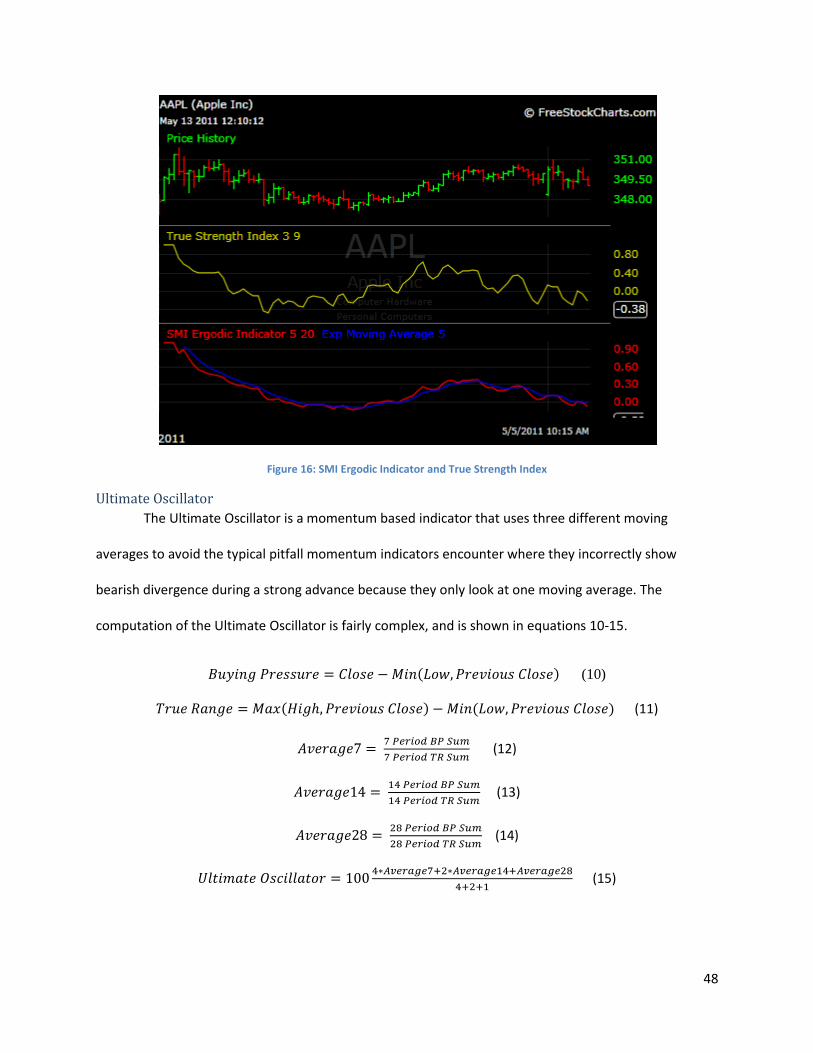
48
Figure 16: SMI Ergodic Indicator and True Strength Index
Ultimate Oscillator
The Ultimate Oscillator is a momentum based indicator that uses three different moving
averages to avoid the typical pitfall momentum indicators encounter where they incorrectly show
bearish divergence during a strong advance because they only look at one moving average. The
computation of the Ultimate Oscillator is fairly complex, and is shown in equations 10-15.
(10)
(11)
(12)
(13)
(14)
(15)
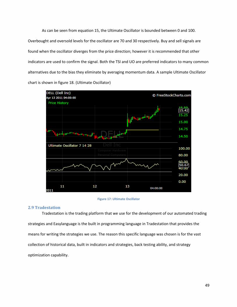
49
As can be seen from equation 15, the Ultimate Oscillator is bounded between 0 and 100.
Overbought and oversold levels for the oscillator are 70 and 30 respectively. Buy and sell signals are
found when the oscillator diverges from the price direction; however it is recommended that other
indicators are used to confirm the signal. Both the TSI and UO are preferred indicators to many common
alternatives due to the bias they eliminate by averaging momentum data. A sample Ultimate Oscillator
chart is shown in figure 18. (Ultimate Oscillator)
Figure 17: Ultimate Oscillator
2.9 Tradestation
Tradestation is the trading platform that we use for the development of our automated trading
strategies and Easylanguage is the built in programming language in Tradestation that provides the
means for writing the strategies we use. The reason this specific language was chosen is for the vast
collection of historical data, built in indicators and strategies, back testing ability, and strategy
optimization capability.
50
2.9.1 Strategies
The main feature of Tradestation that we use is the strategy building section of Easylanguage
which is the place where we write trading strategies. In these strategies we are able to access any prior
price or volume data, indicator data, custom made functions, and fundamental data. Using all of this
data, we can verify any of the common buy or sell signals such as crossovers, indicator levels, time of
day, and to some extent news announcements. The limit to news announcements is that we can only
determine when a news announcement occurs, but not interpret the message. As a result, we simply
shut down our strategies in the period immediately following the announcement. See the appendices
for examples of the strategies we develop.
2.9.2 Indicators and ShowMes
Two tools in Tradestation that are helpful for traders but not as useful for automated trading
strategies are indicators and ShowMes. They allow the user to plot indicator charts for either custom or
built in indicators on asset charts, or in the case of ShowMes they identify points on the asset chart
where certain criteria are met. These capabilities can be useful for testing the indicators and criteria that
our strategies will be using. Aside from this feature though, indicators and ShowMes are of little use to
us.
2.9.3 Back testing
Historical back testing is one of the most important features offered in Tradestation and the one
that sets it apart from other trading platforms. We have the ability to apply our strategy for any amount
of previous data for every stock or currency and receive a great number of statistics on our trading.
Some of these statistics include total profit, percent of profitable trades, average size of winning and
losing trades, average number of bars a position was held on to for, and details of each individual trade.
These statistics are essential for analyzing strategies and improving their performance, although not
quite as useful as the strategy optimizer.
51
2.9.4 Strategy Optimization
Strategy optimization is a very important part of our work and we will go into great detail with it
later in the paper, but for now we will give a brief overview of the basic functions of Tradestation’s
strategy optimizer. The strategy optimizer allows the user to apply their strategy to a set of price data
for an asset over a given period of time, and the optimizer determines a set of optimal parameters. The
parameters can be optimized to yield the largest profit, the highest percentage of profitable trades, or
one of several other statistics. Optimal parameters are a significant component to developing effective
strategies and are a major issue that we focus on in our work.
2.9.5 Data Exportation
During our research we looked at finding a way to export calculations and data to another
program, such as MATLAB or Microsoft Excel, to try to accelerate the speed of calculations. While there
is at least one product available that does this, it was questionable if it is still supported in the current
versions of Tradestation, so we did not invest in it. In a future project we hope to be able to write such a
program.
52
3. Trading Plans, Journals, and Equity Charts
3.1 Trading Plan
It is the summary of the overall goals of the trader or investor. In a trading plan, the trader will
start off by recording how much capital is to be invested. Then a desired long-term return on the
investment is recorded as well as the methods and approaches that the trader will take in order to
achieve his or her desired goal. In this plan, the trader should also outline how much capital he or she
will chose to reinvest into gaining more leverage and how much should be saved.
3.2 Trading Journal
A trading journal allows a trader to scrutinize his trades after they have been carried out. It
should include an observation and description of market movement, a formulation of hypothesis to
explain the movement, and finally the use of the aforementioned hypothesis to predict new
movements. The journal should also contain other information such as the emotional state during the
period of trading and any interesting ideas pertinent to the market that the trader may conceive. Also
included should be reason for any entries and exits as well as events that may have an effect on the
market.
3.3 Equity Charts
They are the charts that contain information regarding all trades and their profit or loss. These
can then be periodically examined to check if profits and losses are within normal distribution. Plots can
be made from the moving average profit factor over the last 20 trades to determine the sustained
success of a system as well as a means to quickly identify potential problems or shortcomings in the
system as time progresses.
53
4. Algorithm from Tradestation Labs Tradestation Labs provides several premade strategies that can be downloaded and used by
anyone, so we worked with one of them and made some modifications to improve its' performance.
This strategy was not a primary focus of the project, but rather good preparation for developing
algorithms of our own.
4.1 Contrarian Z-Score Algorithm The Contrarian Z-Score Algorithm finds the Z-Score of the current stock price based on the last
10 bars, and also the momentum of the average Z-Score based on the last 5 bars, then uses that data to
generate buy and sell signals. Users are instructed to buy when the average Z-Score is negative, and sell
when it is positive. (Guevara, 2010)
We will briefly summarize performance results here. At first we tested the algorithm on AAPL,
RIMM, and GOOG, for 2 minute, 10 minute, and 1 day bars. The pattern seemed to be that the shorter
bar intervals were more profitable, and the longer the bar interval got the less profitable the strategy
was. The irony of this is that the strategy description from its author stated that the strategy works
better on longer bar intervals, so this result was surprising.
One minor modification to the buy and sell signals drastically improved the performance of the
algorithm on 1 day bars, but didn't have a clear impact on the shorter term strategies. The modified buy
and sell signals are to buy when the average Z-Score momentum is negative and the current price is
small than the average price minus one standard deviation, and sell when the Average Z-Score
momentum is positive and the current price is larger than the average price plus one standard deviation.
Again, we offer a brief summary of the full results, but as mentioned, the new results are
significantly better results than the unmodified strategy returned because we are now being more
selective on when we open a position. One interesting observation about both the modified and
54
unmodified algorithm is that in almost every case observed either the long or the short positions would
yield a large profit, while the other would yield a loss. Further investigation into this problem should be
done because if we can find a way to have profitable results for both our long and short positions then
this algorithm would be very profitable overall. Another observation is that the average number of bars
a position was open in losing trades was always significantly larger than it was in winning trades. To
combat this, it would help to add an exit condition based on the number of bars since the position was
opened.

55
5. Slope Calculating Algorithm
5.1 Overview This algorithm predicts trends in the price movement of a stock by looking at the slopes of the
price at different bar intervals. The strategy will first calculate the average rate of change of the closing
price over the last 5 bars for a 1, 5, and 10 minute time interval, call the slopes a, b, and c respectively.
The idea is that the shorter bar interval slopes will reflect changing trends faster than the others, but are
much less accurate. Therefore, we require a sufficient deviation between the slopes before we open a
position. Further, we compare the current close price to the highs or lows over the last 30 or so bars(1
minute bars) to make sure it is sufficiently close to them to be worth investing in. Specifically, buy and
sell signals are determined as shown in equations 16 and 17 respectively, and exit conditions are shown
in equations 18 and 19.
>
>
for d,e,f parameters with d > e > f AND
(16)
<
<
AND
(17)
(Profit percent > .2) OR (bars_since_entry > 15 AND Profit percent > .05) OR (Profit percent < -.15) (18)
These parameters were not optimized exactly, but rather tested approximately against several
different stocks to yield results that are generally profitable. Also considered was adding on a fourth and
maybe fifth bar interval to see if that would be more accurate at predicting trends. Several problems
were observed throughout the testing process so the algorithm was altered drastically throughout our
work.
5.2 Improvements The first realization made was that in markets consistently trending in a certain direction, one of
the two types of opening positions would underperform. For example, when trading AAPL, which has
56
been reliably increasing in price, short positions were almost always losing money. To counteract this
issue, we sought a way to detect when a market is trending in a certain direction. The ideal way to
detect a trend is to look at the price movement of the stock over a fairly long period of time, such as the
previous year or month. Unfortunately Tradestation only provides access to a few High, Low, Open and
Close prices over these large time gaps, so we were forced to work with that data. We compare the
current weekly and monthly critical points to the optimal values of the previous week and month. We
only allow long positions to be opened if the current weekly and monthly high values are greater than
the previous weekly and monthly high values. This shows that the stock has been performing better
recently than it was previously, so it is most likely on an upward trend. Similarly, to open short positions
we require that the current weekly and monthly low price values are lower than the previous low points.
These criteria make it unlikely that both long and short positions will be made at the same time for a
given equity, but they have been dependably providing positive results, so it seems that this may be an
ideal approach. Something that could be added later is a check to see if the current price is still within a
reasonable range of the observed critical points, so in the event that a stock reached a global critical
point and immediately started trending in the opposite direction, we would be protected.
Also, it should be noted that the weekly and monthly critical points can be misleading if it is very
early in the week or month. For example, if we check the weekly high value on Monday at 10 AM, there
is almost no price data for the week so the high value will tell us very little about the price trend. We
implemented a mechanism to prevent this by checking the day of the week and the month, and if we
are too early into the time interval, we compare critical values of one period ago to those of two periods
ago. The exact check performed is to see if it is at least Wednesday, and at least seven days into a new
month. This assures that there will be plenty of data in the sample from which we draw our critical
points.

57
We also tested an alternative way of detecting trends based on the change in the closing price.
The closing price at the beginning of the chart was compared to one in the middle of the chart, and then
the middle value was compared to the current closing price. To be able to open long positions it was
required that these three values be ascending, showing that the price has been going upward over the
observed time period. For opening short positions the constraint was that the three values be
descending, so the stock price has been on a downward slope over time. The difference in this approach
is that it detects trends over a shorter time interval while the other method detects long term trends,
assuming the user is looking at an intraday chart.
Both of these tests tell the user different information about the stock, so the ideal strategy may
be to use both. The longer term trend data not only tells the user where the stock is likely to be headed
in the distant future, but also it gives an idea of how traders will react to certain price changes. For
example, if AAPL takes a sharp downward turn over the course of an hour, then traders will look at the
chart and probably decide to buy the stock since AAPL has been so dependable in increasing recently,
and their buying the stock will in fact force the price back up. In that example we see that a long term
trend can actually be used to predict a short time price movement. The shorter term price data is less
reliable due to the volatility of the market, so while it helps to consider, it will often send the opposite
sign about where the price is going. An example of this would be a price that has a strong upward trend
until it reaches a global maximum, but this trend conflicts with the long term trend of the equity. In this
case investors would believe that the high price precludes a major price drop coming soon, so they short
their shares before the fall, which in turn makes the price fall. It seems like the ideal way to use the two
types of trend data would be to compare the two, and if they match, then the price is probably heading
in that direction, but if they disagree then follow the direction of the long term trend. Technical
indicators are often built based on this idea, and could also be used for predicting trends.
58
Following many attempts at finding an ideal market for the shorting algorithm approach, we
were unable to determine many markets with long term downward trends. Despite experimenting with
several tests for determining appropriate conditions for applying the algorithm, we could not find a test
that consistently worked. As a result, we decided only to continue work on the long position portion of
the algorithm.
While we used the averages of the recent slopes at each bar interval, some other methods for
computing the predicted trends were considered. Another possible approach to our problem that was
suggested but not examined is to use an exponential average giving greater weight to recent slopes over
older ones when calculating the final averaged slope. That way recent trends would become more
visible in less time, which is exactly what a successful trader should want. One more approach would be
simply to calculate one slope between the closing price five bars ago and the current price, so that the
slope shows exactly how the price has moved overall in that time period. This method would give a
clearer picture of longer term movements in the price, but not as good an idea of how volatile the price
movements are between bars.
One problem that was noticed almost immediately was that positions that remained open at the
end of the day were extremely dangerous because the opening price the next day is generally drastically
different than the closing price. While this sometimes led to significant gains, it more frequently resulted
in major losses, so we decided to seek a way to try and avoid having open positions at the end of the
day. To solve this problem, we limited the algorithm by closing any remaining open positions at 3:59.
The difficulty in implementing this change is that it makes it impossible to simultaneously apply the
algorithm to the stock market and the Forex market because they have different business days, so we
must be wary of this when switching between markets. The benefit of the change certainly did not go
unnoticed, as it successfully filtered out major losing trades caused by open positions carrying over to
59
the next day. An alternative solution to the problem would simply be not open any new trades after a
certain point chosen to guarantee that there would almost never be open positions at the day end. We
investigated this approach, but decided that the ideal solution would be to try and predict the major
volatility swing at the opening of the next day.
Since this algorithm trades so frequently, the assumption we took in approaching the multi day
trading strategy was that stock prices oscillate in one range. While this assumption would not be true
over long periods of time because stock prices tend upward, in a matter of a few days it is generally true
that a stock will stay within similar bounds that it did the day before. Therefore, we first calculated the
percent change in the stock from the days open to the current time (3:59PM). The algorithm closes our
position if the percent change was anywhere above -.5%. However, if the stocks percent change in price
was anywhere below that level, we anticipate its price rebounding at opening the next day, so we either
hold our open position or open a new long position. This approach proved to be quite successful at
turning what had previously been a problem into a significant source of profit.
Due to the success of strategic days end trading we decided to also attempt to profit from it by
looking at the stock in its first minute of opening. It was observed that when the first one minute bar of
the day closes higher than it opened, the next few bars do the same. To capitalize on this pattern, we
compute the net change in price over the first bar and immediately buy the stock if the net change is
positive, or hold a long position if we already have one. This was yet another simple way we were able
to capitalize on simple market patterns.
One more change made in the algorithm was to not only look at the first derivative of the stock
prices, but also to consider the second derivatives. The reasoning behind this was so that we can look at
how the stock price is changing more carefully. The first derivative tells us how fast the stock price is
changing, but the second derivative tells us the direction of the price changes. Upward trends rarely

60
transition from major price increases to major price decreases without any steps in between. Rather it is
more likely that the price will increase rapidly, then will start to increase at a slower rate before it
ultimately starts trending downward. By looking at the second derivative, we can see when these
increases start to level off and use that information to better decide when it is time to short the stock.
Likewise, we can use second derivative information to decide when a downward trend is about to be
reversed so we should buy the stock.
We calculate the second derivatives exactly the same way that we found the first derivatives,
except we replace the closing prices in the formula with the first derivatives. The second derivatives are
then added into our buying condition, where we require the short term second derivatives to be greater
than the longer term ones to open a position. Larger values for short term second derivatives symbolizes
the fact that the price increases are getting more drastic in the recent periods, so a large upward trend
is likely to be coming soon and it would be profitable to open a long position. For the short position we
look for the shorter term second derivatives to be smaller(more negative) than the longer term ones.
That tells us that recent price decreases are more drastic, so the downward trend is gaining strength and
that opening a short position will be profitable.
5.3 Conclusion Overall the algorithm has proved to be consistently profitable through simulations; however,
there are several concerns. The main issue perceived in the algorithm is that it trades so frequently that
it is more susceptible to certain factors. The first of these is simply the transaction costs, which using
Tradestation amount to 1 cent per share of stock bought, which makes marginal profits generated on
the one minute bar intervals even less. Trading on such short intervals means that we will need to trade
more to make a large profit, but more trades means more transaction costs, so that issue is inherent in
this approach. Also inhibiting the profitability of the algorithm is the bid-ask spread that could not be
accounted for in our performance testing of the algorithm. Since we are making a very small profit on

61
many trades, it is difficult to guarantee that profits will be sufficiently large to cover the bid-ask spread
discrepancy in our profit calculation. Despite these issues, we remain confident that with the proper
attention to determining ideal parameters this algorithm could be made to be very profitable.
62
6. Factor Weight Algorithm
6.1 Overview The goal of this algorithm is to weight different factors that can be used to predict price changes
in a stock, and combine them all in to one expectation for the future price. These factors can come in
the form of fundamental data, technical indicators, mathematical models, binary data, temporal data,
price changes of similar assets and anything else that can be expressed in numerical form. At its
simplest level the algorithm will be a linear combination of these different factors, with each factor
weighted based on its accuracy in predicting price changes in the past. As the algorithm is tested further,
we hope it will evolve beyond a linear equation to something that may fit the data better, if necessary.
6.2 Factors Used As a starting point we began with a few basic overbought/oversold technical indicators. These
indicators are all a single line based on previous price and volume data that attempt to predict price
movements in an asset by finding patterns in the way the asset is being traded. Several of these
indicators are briefly described below.
Commodity Channel Index(CCI): Designed to determine cyclical turns in the price of a
commodity(or stock), the CCI is set so that when it’s value is high (above 100 is a common signal) the
asset is in an uptrend signaling to traders that they should buy the asset, and when the asset when it
takes on low negative values (below -100 is a common signal) traders should sell the stock. We will
investigate both using this indicator literally and using it for binary data (1 if it is outside of the itnterval
(100, -100), 0 otherwise.) to optimize algorithm performance.
Elliott Wave Oscillator (EWO): The Elliott Wave Oscillator is a 34 period moving average of prices
subtracted from a 5 period moving average of prices. While typically this oscillator is used to identify the
location of points for traders using Elliott Wave Theory, we will use it as another overbought/oversold

63
oscillator. High values of the oscillator tend to indicate a potential price decrease, while low values for
the indicator generally precipitate a price increase.
Elder Ray Bear/Bull Power(ERBeP/ERBuP): The Elder Ray Bear Power Indicator is calculated by
subtracting the exponential moving average(EMA) of closing prices from either the high or low price of
the day (high for Bear, low for Bull). Both indicators are usually used with the slope of the EMA, so that
may also be a factor in our equation. These indicators in a basic sense show the power(volume) of
bearish and bullish traders respectively. When the ERBeP takes on a large value, there is a lot of bear
power in the market, meaning traders are pessimistic of where asset is going, so it is likely to fall soon.
When the ERBuP takes on a large value, it is likely that the stock price will witness an upward trend in
the near future.
There are many other indicators that can be applied to our algorithm, and for ideal accuracy we
hope to apply as many of them as possible. Again, any technical indicator that can output a single
numerical value can be used with the algorithm to predict stock prices. There are several other forms of
data that we hope to apply to our algorithm to add valuable information about price trends.
Fundamental data about companies is often used by traders to back up any theories drawn from
technical indicators about future price movements. So too will we use fundamental data to support our
algorithm. Since we plan to ultimately have a completely automated trade strategy, we account for the
fact that there will be no human to double check what our algorithm is doing. Therefore, we present
several fields of fundamental data into our equation to automate this process. To elaborate on this, is it
reasonable to expect a major stock price increase in a company that had a very negative net income one
period ago? Therefore, accounting for important company details such as the company’s recent net
income can help to alleviate concerns about the automated process making illogical decisions based
solely on technical indicators. Below are a few more examples of fundamental data for stocks that we
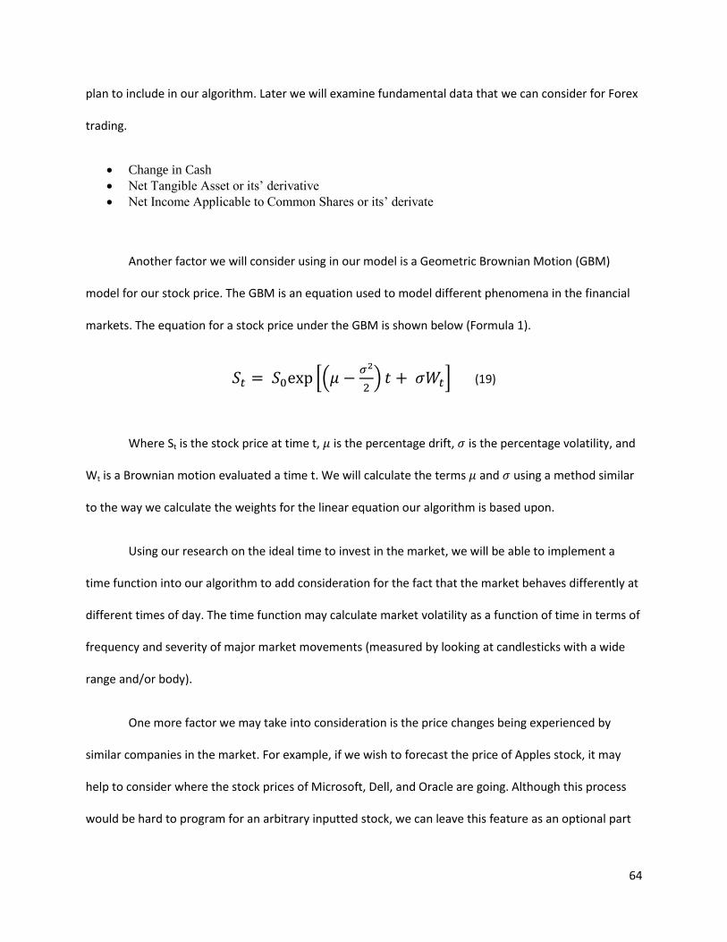
64
plan to include in our algorithm. Later we will examine fundamental data that we can consider for Forex
trading.
Change in Cash
Net Tangible Asset or its’ derivative
Net Income Applicable to Common Shares or its’ derivate
Another factor we will consider using in our model is a Geometric Brownian Motion (GBM)
model for our stock price. The GBM is an equation used to model different phenomena in the financial
markets. The equation for a stock price under the GBM is shown below (Formula 1).
*(
) + (19)
Where St is the stock price at time t, is the percentage drift, is the percentage volatility, and
Wt is a Brownian motion evaluated a time t. We will calculate the terms and using a method similar
to the way we calculate the weights for the linear equation our algorithm is based upon.
Using our research on the ideal time to invest in the market, we will be able to implement a
time function into our algorithm to add consideration for the fact that the market behaves differently at
different times of day. The time function may calculate market volatility as a function of time in terms of
frequency and severity of major market movements (measured by looking at candlesticks with a wide
range and/or body).
One more factor we may take into consideration is the price changes being experienced by
similar companies in the market. For example, if we wish to forecast the price of Apples stock, it may
help to consider where the stock prices of Microsoft, Dell, and Oracle are going. Although this process
would be hard to program for an arbitrary inputted stock, we can leave this feature as an optional part
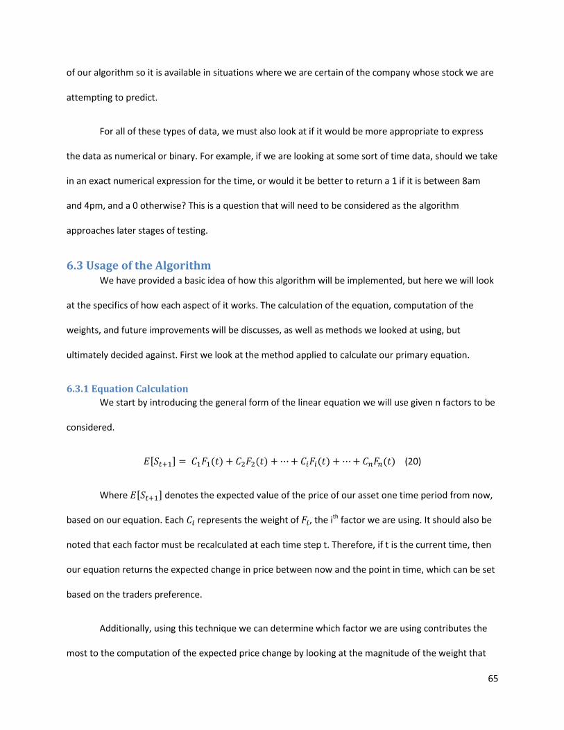
65
of our algorithm so it is available in situations where we are certain of the company whose stock we are
attempting to predict.
For all of these types of data, we must also look at if it would be more appropriate to express
the data as numerical or binary. For example, if we are looking at some sort of time data, should we take
in an exact numerical expression for the time, or would it be better to return a 1 if it is between 8am
and 4pm, and a 0 otherwise? This is a question that will need to be considered as the algorithm
approaches later stages of testing.
6.3 Usage of the Algorithm We have provided a basic idea of how this algorithm will be implemented, but here we will look
at the specifics of how each aspect of it works. The calculation of the equation, computation of the
weights, and future improvements will be discusses, as well as methods we looked at using, but
ultimately decided against. First we look at the method applied to calculate our primary equation.
6.3.1 Equation Calculation
We start by introducing the general form of the linear equation we will use given n factors to be
considered.
[ ] (20)
Where [ ] denotes the expected value of the price of our asset one time period from now,
based on our equation. Each represents the weight of , the ith factor we are using. It should also be
noted that each factor must be recalculated at each time step t. Therefore, if t is the current time, then
our equation returns the expected change in price between now and the point in time, which can be set
based on the traders preference.
Additionally, using this technique we can determine which factor we are using contributes the
most to the computation of the expected price change by looking at the magnitude of the weight that
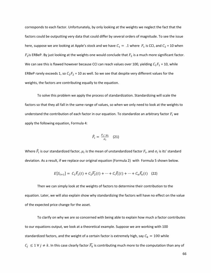
66
corresponds to each factor. Unfortunately, by only looking at the weights we neglect the fact that the
factors could be outputting very data that could differ by several orders of magnitude. To see the issue
here, suppose we are looking at Apple’s stock and we have where is CCI, and = 10 when
is ERBeP. By just looking at the weights one would conclude that is a much more significant factor.
We can see this is flawed however because CCI can reach values over 100, yielding = 10, while
ERBeP rarely exceeds 1, so = 10 as well. So we see that despite very different values for the
weights, the factors are contributing equally to the equation.
To solve this problem we apply the process of standardization. Standardizing will scale the
factors so that they all fall in the same range of values, so when we only need to look at the weights to
understand the contribution of each factor in our equation. To standardize an arbitrary factor we
apply the following equation, Formula 4:
(21)
Where is our standardized factor, is the mean of unstandardized factor , and is its’ standard
deviation. As a result, if we replace our original equation (Formula 2) with Formula 5 shown below.
[ ] (22)
Then we can simply look at the weights of factors to determine their contribution to the
equation. Later, we will also explain show why standardizing the factors will have no effect on the value
of the expected price change for the asset.
To clarify on why we are so concerned with being able to explain how much a factor contributes
to our equations output, we look at a theoretical example. Suppose we are working with 100
standardized factors, and the weight of a certain factor is extremely high, say while
. In this case clearly factor is contributing much more to the computation than any of
67
the other factors. The conclusion one can draw from this is that either that one factor is extremely good
at predicting price changes, or that the other 99 factors are contributing almost nothing. In practice it is
unlikely that we will choose 99 factors that are so much worse than one factor, so it is probable that
there is some error in the computation of the weights. So we can see that standardizing the factors is
useful in helping identify potential errors in our code.
A particular use of standardization is for improving our model. If we see that a certain factor is
weighted more heavily than others on a consistent basis, we may be able to improve our model by
replacing the linear function with something of a higher growth rate. For example, if is much larger
than the other weights, then we can replace with some function of , perhaps which has a higher
growth rate. This would be a fitting replacement if grows so fast that modeling it with a linear
equation is inaccurate. Likewise if we had a consistently small weight, we could replace its’ factor with a
function that grows more slowly, like replacing with . In this case standardizing our factors and
paying attentions to the weights can help the accuracy of our algorithm as it develops.
Now that we have seen extensively how our main equation is calculated and how it can be
interpreted, we direct our attention to the challenging problem of actually computing the weights.
6.3.2 Weight Parameter Estimation
It is very unlikely that coefficients exist that fit our model to the data exactly, so instead we will
investigate numerical methods that can approximate the weights. This process requires three separate
functions. The first one must simply calculate the equation as shown above. The second function will
subtract the values returned by the equation over the last X+1 bars from the actual price changes over
the last X bars, square the differences, then sum them. The third function will minimize the output of
another function by finding the ideal inputs to it, which in this case are our weights. We will examine the
way each of these functions to determine the ideal approach to each.
68
The first function is the most straightforward of them all. All we require it to do is complete the
calculation of the expected change in price for the next time step, given a certain starting change in
price for the next time step, given a certain starting point. We require the function to output the
expected price change, and we may also consider having it output the time step to avoid errors in later
functions.
The second function serves to compute the correlation between the equation and the actual
price changes. We align the computed price change with the actual price change experiences for a given
number of recent bars. A difficult question to consider here is what price we should compute. We could
do this process for each price on a candlestick (high, low, open, and close), so we have an expected
value for each of these. The problem with this approach is that it would require four times as many
approximations, so it would slow down the code significantly. Other ideas to be considered are to look
at the mean of the candlestick points, or the norm of them. It is believed that these two options would
run faster, but be less accurate. Future analysis will be performed to identify an appropriate option that
is the best balance of speed and accuracy for our purposes. Regardless of this choice, we will ultimately
compute the sum of the squares of the differences between our predicted price changes and the actual
price changes. This value essentially tells us how far off our predicted prices are from the actual price
changes, so we want to minimize this function.
To perform this minimization we need to develop a multivariate optimization algorithm. Once
we have a function that can minimize our second function, we can determine our ideal weights for our
equation. Again we must consider the fact that our algorithm will be running on its own without the
chance for human intervention, so our minimization algorithm must be able to work accurately and
efficiently so our trading results do not suffer. Below we discuss the optimization methods considered
for use in our code.
69
The Nelder-Meade Algorithm is a common choice for minimization problems. Despite the
frequent use however, it is immediately unappealing for our purposes because it is designed for
unimodal functions. The issue that arises with this is that when applied to a multimodal function, it
frequently converges to a local minimum rather than the global one. In our context, this means that we
would get a set of weights that are suboptimal fits for our equation. Since we require optimal accuracy,
this issue is not acceptable so we must consider other optimization schemes.
The Simulated Annealing algorithm was researched and served as the basis for the algorithm we
develop. This algorithm is ideal for finding the global minimum of a function with many local minimums.
It is designed specifically to get away from local minimums as it iterates. We plan to implement this
algorithm at a later date to compare it’s efficiency with the one we develop below.
Another option considered but not tested was to replace the optimization algorithm with an
Extended Kalman Filter, and use that to filter our equation and historical data together to both estimate
the weight values and ultimately produce a more accurate equation for the expected change in price at
the next bar. This option was neglected because it seems that to produce accurate parameter estimates
the filter would require a large amount of data points. The reason this is a problem is because obtaining
all of that data would involve tracing the market back a long time, so we risk basing our estimates off of
data from a market experiencing very different conditions than the current market is in. However, it is
still a future goal of this project to be able to implement the Extended Kalman Filter and compare the
accuracy of its results and its runtime to the current method.
Due to a lack of prominent optimization algorithms for multimodal systems, we decided to
design our own approach to the problem. The basis for our approach is to take a very large sample of
points over the interval where we expect to values of the weights to range, then find the minimum
among those points, zoom in on that, then repeat the process until we are very close to a global
70
minimum. Our initial assumption was that the weights will fall somewhere in the interval (-100, 100), so
our algorithm starts by generating 10000 random points in that interval, evaluating our equation at each
of them, then finding the point with the minimum value. Once we have that point, we make it the
center of our interval; shrink the size of our interval while still taking 10000 random points in it, then
repeat the process. Preliminary testing of this algorithm in MATLAB found that it could compute the
minimum of a multivariate function in about half a second with an error of less than 10-5. This is largely
due to the stopping condition we added which terminates the algorithm when it iterates 10 consecutive
times without finding a smaller minimum. Having found an algorithm that is both fast and accurate, we
can begin to link our functions together to create our automated trading strategy.
6.3.3 Equation Implementation
Once we have our equation with optimal weights determined we can accurately predict where
the price of the stock is going. So what we do is take the current values for all of the factors we are using
and plug them in to our first function to compute the expected change in price by the end of the next
time interval. The next step varies based on whether we choose to estimate all of the points in the
candlestick or just the mean or norm of them.
Let us suppose we just have the expected change in the mean of candlesticks. We are interested
in buying when this value is very high, and selling when it is very low. Therefore, we must devise a way
of automating this decision so the algorithm can decide for itself what “very high” and “very low” mean
exactly, and act accordingly.
One method for doing this would be to find the mean and standard deviation of price
changes over the past few bars, then we can say if the current expected price change falls outside of the
interval ( then we should buy or sell based on which side of the interval our point is on.
Another thing we can optimize for this approach is what multiple of we should use to determine
71
appropriate bounds for the interval. The larger the multiple is, the less trades we will engage in, but the
more profitable they will be. Conversely, choosing smaller intervals will lead to more, less profitable,
trades. This problem is something we can solve by estimating the multiples in a manner similar to the
way we estimated the weights for our equation. It would be inefficient to repeat this process every time
we trade however, so it may be wiser to do one experiment with a great deal of historical data to
calculate an appropriate value for the interval then stick with that number.
Another approach we can take to choosing when to long or short stocks is to compare a current
expected price change to the last X of them, and if it is either the maximum or the minimum then we
long or short accordingly. Here we again run into a problem where we would need to decide how many
bars back we should go to compare our price change expectation. Similarly to before, we have a tradeoff
between quality and quantity. The more bars we look at, the less likely we are to trade, but the more
profitable our trades will be. The contrast being that less bars will lead to more trades and less profit per
trade. Once again, we have a number X that we can attempt to optimize for profit.
Yet another approach could be to choose constant bounds for the expected price change, and
buy or sell when we go outside of the bounds. Similar to the other cases, we have to answer the
question of how to choose these bounds. Once more, we can use backtesting to optimize these bounds
for our profit then use them going forward.
It is hard to say if any of these approaches is any better or worse than one another without
extensive testing which needs to be performed using all of them. In each case we have an additional
parameter we need to estimate just like we had to estimate the weights for our equation. A potential
issue that may arise both with our equation and with these bounds is how often should we recalculate
our parameters. To answer this question we need detailed information about the run time of the
optimization to see how much delay it adds to our trading strategy. If it is somehow possible to

72
recalculate these bounds independently while our algorithm continues to run using the previous
bounds, that seems like it would be the ideal scenario because then we could constantly recalculate the
bounds for optimal accuracy without suffering any delay in our trading.
Now that we have a long or short position in our asset, we must determine when it is an
appropriate time to close our position. It is our hope that our price change predicting algorithm can
again be applied to answer this question. Without much investigation, one can see that this problem
closely resembles the one previously encountered. Once we have opened our position, we want to look
for when the price change is expected to go in the opposite direction, or when it is close enough to
changing direction that we should close our position. If we have a long position, then we want to set a
lower bound on the expected price change, so that when it goes below that lower bound we should
close our position. Likewise if we have an open short position, then we want to place some sort of upper
bound on the price change so that we can optimize our profits.
Another factor to consider is the profit we can make by closing a position at the current time.
While the expected price change may still be in our favor, we must also consider that the risk in staying
in a position is relative to the profit we could have by exiting at the current time. If we could close a
position and make 2 million dollars, the risk of loss is much greater than a situation where closing the
position would lead to a 200 dollar gain. Likewise, we must also consider a bound on our losses in the
event of a losing investment. Just as before these bounds need to be computer and factored into our
calculation so that we can maximize our profits. Once again we will look to back testing to provide us
with an optimal choice of bounds to maximize our profits.
6.4 Potential Errors Now that we have seen how to build the algorithm from the ground up as well as how to
automate it into a dynamic trading strategy, we will look at potential errors our strategy may encounter.

73
To this point, we have discovered one major problem that inhibits our program severely. This major
problem is the occurrence of major events in the world that strongly influence traders. Almost every
trading platform now lists major news announcements involving companies when displaying their stocks
information. Upon immediate inspection one can observe that with these news announcements usually
comes a drastic change in the stock price.
We begin to experiment with ways in which we can avoid this problem in our strategy. Our first
approach was to search for some function that allows us to immediately disable our strategy when a
news announcement comes out. We were able to find an EasyLanguage function called NewsCount
which provides the number of news headlines for a stock in the current day. This function allows us the
luxury of checking for any new news announcements at any bar. Once we are aware of a news
announcement we can tell stop our strategy from opening any new positions for 2 bars which should
provide due time for the stock price to level out. In order to deal with already open positions we
propose using the price bound technique, but setting the bar in the loss direction much smaller so in the
event of a news announcement that drives the stock in the direction we don’t want it to go, we can
minimize our losses. We may also consider setting the profit bound higher since a news announcement
in our favor could lead to a very profitable opportunity. To properly determine appropriate bounds we
must yet again look to back testing and calculate optimal bounds for when we have open positions at
the time of a news announcement.
A risky but potentially profitable alternative to sitting out for 2 bars after a news announcement
would be to set up yet another set of bounds for the case where we do not have an open position at the
time of a news announcement. Due to the high risk of these sort of trades however a large amount of
back testing of this type of strategy would be required. Even with a great deal of testing it is probable
that an effective strategy cannot be derived due to the extreme randomness present in these

74
announcements. Unfortunately this may just be a case where the human decision making is
irreplaceable by an automated strategy.
Another issue we may encounter with our algorithm has already been alluded to; the issue with
not being able to recalculate the optimal parameters constantly. Since prices are constantly changing we
would ideally update our parameters continuously, however the speed of our algorithm does not allow
for that. We will spend much time working to optimize the efficiency of our algorithm, but the high
volume of calculations required makes elongated computation time inevitable. This problem forces us to
consider the aforementioned alternative methods for parameter estimation such as the Simulated
Annealing optimization algorithm and the Extended Kalman Filter.

75
7. Indicator Scorecard Algorithm
7.1 Overview This algorithm was developed with strong influence from the Factor Weight Algorithm. The basis
for this algorithm is to look at several factors regarding the asset price, whether it is overbought or
oversold, its volatility, and the type of trend it is following. For each piece of data we apply technical
indicators to apply to an overall equation that determines whether or not it is a good time to open a
long position. These indicators are normalized and put into a linear equation that generates a numerical
value that will achieve high values when it is an appropriate time to buy the asset. The equation is given
by Formula 6.
(23)
Where each is a normalized indicator and each is its corresponding weight coefficient. A is
the value indicating the strength of the buy signal generated by the equation.
For overbought/oversold information two indicators were used, CCI and RSI. Each indicator is
oversold when it achieves low values, so the coefficients corresponding to these indicators take on
negative values. These inputs will simply suggest when a price increase is likely to come in the future but
offer little in regard to the magnitude or duration of the price change.
To understand magnitude and trend information we use the volatility indicator Average True
Range in our equation so that when we invest before price changes, we will know the price changes will
be large enough to generate sufficient profit. ATR takes on larger values when the volatility is higher, so
it is reasonable that our coefficient for this indicator will be a positive one, because we want our buy
signals to be stronger when the asset price changes are more drastic since that is when we can make
larger profits.

76
The last indicator applied is one that looks at the strength of trends currently facing the asset
price. At first thought it would seem that strong price trends would be ideal for investing, but testing
revealed that the opposite is true. Working with the ADX indicator, which takes on higher values when
price trends are stronger, our optimization showed that the best corresponding coefficient would be
negative, so weaker price trends are better for investing. Perhaps this can be interpreted as showing
that markets that are oscillating frequently offer more opportunities to invest profitably.
Testing was done on 15 minute bars to make it so that the algorithm would perform less trades,
which will optimize its profit with respect to exchange commissions paid on each transaction. Further
accounting for these commissions, the optimization assumed an exchange commission of $.01 per share
per trade taken into account to further account for the exchange commission's encountered in real
trading.
As for exit conditions, a fairly standard set of computations are done to exit when profit is high,
or to avoid a large loss. Six numbers are optimized to provide the best set of exit conditions, and they
are:
MaxProfit: A profit margin that is sufficiently large to close the position.
MaxProfitlong and Longprofitwait: A profit level which if reached after waiting so long will signal a time
to exit.
MaxLoss: A loss large enough to trigger an exit from the position before more loss is sustained.
Maxlossshort + Shortlosswait: If the position has been open long enough and this loss is sustained, an
exit sign is triggered.
To summarize this, we will exit quickly if we have reached an desired profit or a loss, or after
having an open position for a long period of time, we will exit at lower profit/loss thresholds.

77
7.2 Alternative Approach to Parameter Estimation Perhaps the biggest difference between this algorithm and the Factor Weight Algorithm is the
way in which the two determine the factor weights used in the equation. While the Factor Weight
Algorithm depended on fitting a curve to the experienced price changes, this algorithm determines a
scorecard like metric that suggests how much an investor should want to buy a stock. With this method,
each factor in our equation except for the indicator data is optimized together with the exit conditions
using Tradestation's built in strategy optimization tool to find the set of parameters that will most
strongly relate the algorithm strategy to high profits on investment. The limitations associated with
Tradestation's optimization program do bring about some interesting questions regarding how to make
the best use of it.
The main limitation of the optimizer is that it only allows you to calculate maximum profit based
on one set of data, so only one stock over a relatively short period of time. Surprisingly related to this
issue is the fact that the optimizer is very slow, so it can only work with a small number of possibilities
for parameters at a time. As a result, we developed an approach, which we will refer to as diversified
optimization, which uses the limited number of parameter options as an opportunity to look at more
data sets during optimization.
The way that diversified optimization achieves this is by first selecting a group of data sets to
look at, generally a set of multiple stocks, but if investing in one company it would be more favorable to
look at that companies stock data over different time periods. The next step in the process is to make a
very broad guess at the range in which the parameters fall, and pick a few evenly spaced points in that
range and optimize over that general setting. Next, an alternative data set is brought in and another
range of parameters is computed by observing the new optimal values and creating another range of
values around each parameter, although with a slightly narrower range this time. This process continues
until the parameter values have been computed to such a specific level that any changes make little or

78
no difference in investment strategy (this was found to happen after 7-10 optimizations). A question
that arises in this process is what would be the ideal way to choose the order of data sets analyzed in
the process.
There are several ways to approach this problem, the simplest being to randomly choose an
ordering of the data sets and substitute in data sets during each optimization in that order.
Unfortunately in this case the simple approach is also quite ineffective because simply following an
order that does not change as the optimizer results change will lead to convergence of parameters to
local rather than global extremes in the process of trying to optimize the profit for the overall data set. A
better approach is to look at the profit based on the current parameter set following each optimization,
and then logically decide which stock data set to optimize over next time. This process comes with more
options, such as is the best choice for the next optimization the one which currently yields the smallest
profit, or perhaps the stock whose profit decreased the most during the last optimization.
While the difference in profit amount should be paid careful attention to, only using it to select
the next data set would be hazardous. The reasoning behind this is because after optimizing over a
certain stock, the parameters are most strongly geared toward optimizing that stock, so once they are
optimized over another stock, the first one will almost always see the most drastic repercussions. As a
result, it would seem targeting the stock that suffers the greatest loss or smallest profit is the best
approach to this issue.
Overall this approach generates a more inaccurate equation than the Factor Weight Algorithm
would because the Factor Weight Algorithm did not account for the difficulty of combining stock data
for multiple stocks into one data set, nor did it take into account the slow execution speed of
Tradestation. In the ideal scenario the Factor Weight Algorithm would be superior to the Scorecard
79
Algorithm, but based on the limitations we are forced to deal with the Scorecard Algorithm is the best
we can do, and with enough tweaking it can still be quite effective.
7.3 Results The results of the optimizations revealed some very interesting information regarding the
weights of each of the factors in our equation. It was initially thought that the overbought/oversold
indicators would be the most significant part of the equation, but testing revealed that those indicators
were quite less significant than the other two, particularly the ADX. This conclusion shows that high
levels of volatility and a lack of trends are more indicative of a price increase than the perceived price
trends. It is still possible that the indicators chosen simply aren't indicative of the overall type of
indicators they are representing, but the difference is so staggering that it shouldn't be ignored either.
7.4 Future Work Some future work to be done on this algorithm will attempt to look at a few major unanswered
questions with the algorithm, such as the bar interval being used, the indicators being used, and the
hazards of multiday trading. We have already discussed how day openings generally precipitate large
price movements, so it may be ideal to avoid having open positions before seeing where the price will
go at the beginning of the day, although it is questionable how to combat these situations because they
are so frequent on the larger bar interval. At first the 15 minute bar interval was selected to avoid
trading too often due to short bar intervals and to thus avoid excessive commission payments, but we
will compare this risk to multiday trading risk and come to an optimal conclusion. As has been discussed,
there is a lingering question of which indicators would be the best for the algorithm, and there are so
many different choices that answering that question would be another project all together. Additionally,
adding more indicators into the function may also increase its accuracy but at the cost of the already
quite limited speed of the algorithm. All of these issues can be investigated to improve the overall
performance of the work completed here already.

80
8. Indicator Multi Test Algorithm The Indicator Multi Test Algorithm (IMT) is another slight modification to the Factor Weight
Algorithm. In this version, we take four separate indicators on a 5 minute bar interval and look for when
each of them generate a buy or sell signal, and compute a score based on the strength of each signal.
The four indicators we use are CCI, RSI, Ultimate Oscillator, and Bollinger Bands. The first three each
generate a buy signal when they exceed a certain threshold, so we add a point to our overall score for
each standard deviation above the threshold the indicator reaches, starting from one standard deviation
below it. Equation 24 provides an example of how we add points to the score.
IF [ ] Add i to the score, for i = 1,2,3,4 (24)
The reasoning behind equation 24 is that the CCI deems an asset to be oversold if it takes on a
value below 100. Equation 24 essentially says that the score is increased by 1 if CCI is within one
standard deviation of its oversold level, 2 if it is above the oversold level, 3 if it is far above the oversold
level, and 4 if it is extremely far above it. The same scoring technique is applied to the Ultimate
Oscillator, and RSI. For the Bollinger Bands, we simply add 3 to the score if the asset is below the lower
band and 0 otherwise. When a score of at least 6 is attained, we open a long position.
The exit condition for the algorithm was originally set to wait until the score has returned to 0,
indicating that there is no feeling that the asset is oversold, so it has returned to a normal price. One
problem arose immediately in this in that a single bar does not provide sufficient evidence to signal that
an exit is appropriate. Further, we found that many of the indicators would remain within the extreme
regions for a very long time after entering them, so exits would be delayed excessively. To solve this
problem, the exit condition was altered to close positions if the score is constant for six consecutive
bars. This condition solves both problems previously discussed because it takes into account scores from
81
multiple bars, and will not have the problem of waiting too long for indicator values to be retraced to
their normal range.
Another two conditions are applied to the indicator to help avoid excessively risky transactions.
The first is to check the time to make sure that no positions are opened in the first half hour, or last hour
of the trading period. We do this for the same reason we avoided trading during this time in other
algorithms, the extreme volatility between trading sessions and shortly after a session begins. All
positions are closed at the end of each day regardless of the profit to further ensure that no positions
will be held over multiple days.
One issue that became immediately apparent was that on days when an asset opens much at a
value much higher than it has achieved recently, retracement over the course of the day generates
inaccurate buy signals. Following a very high valued opening price, stocks generally follow a slow
downward trend as they return to their normal range of values. Left alone, the IMT would see the price
decreases immediately and trigger a buy signal when the price was reaching low values for the day, but
an experiences trader would realize that the price decreases are likely to continue until the asset is back
to its normal range, making a long position a very bad investment. We circumvented this problem by
forcing the algorithm to check that the current price is below the average of the high prices from the
previous two days. This solves our problem because it prevents IMT from opening long positions while
the asset is at a relatively high value, so the false buy signals we encountered before won’t be used.
In our usage, this algorithm takes a chickens perspective on trading. A score of 7 is very high and
quite uncommon, so we are really only opening long positions when we can be very confident that they
will be profitable. Further, the exit condition tends to close positions very quickly after opening the
position, so profits are reliable yet small. We could make more trades by lowering the value we require
to open a long position, and hold the positions longer by altering the exit condition.
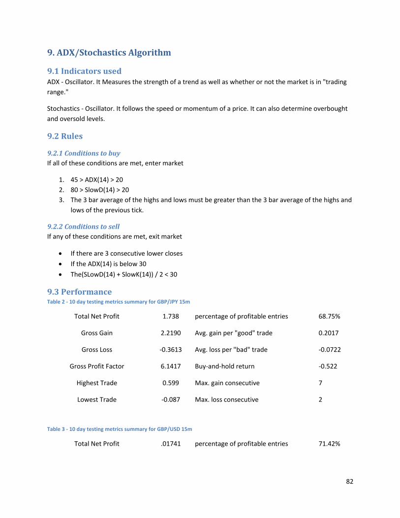
82
9. ADX/Stochastics Algorithm
9.1 Indicators used ADX - Oscillator. It Measures the strength of a trend as well as whether or not the market is in "trading
range."
Stochastics - Oscillator. It follows the speed or momentum of a price. It can also determine overbought
and oversold levels.
9.2 Rules
9.2.1 Conditions to buy
If all of these conditions are met, enter market
1. 45 > ADX(14) > 20
2. 80 > SlowD(14) > 20
3. The 3 bar average of the highs and lows must be greater than the 3 bar average of the highs and
lows of the previous tick.
9.2.2 Conditions to sell
If any of these conditions are met, exit market
If there are 3 consecutive lower closes
If the ADX(14) is below 30
The(SLowD(14) + SlowK(14)) / 2 < 30
9.3 Performance Table 2 - 10 day testing metrics summary for GBP/JPY 15m
Total Net Profit 1.738 percentage of profitable entries 68.75%
Gross Gain 2.2190 Avg. gain per "good" trade 0.2017
Gross Loss -0.3613 Avg. loss per "bad" trade -0.0722
Gross Profit Factor 6.1417 Buy-and-hold return -0.522
Highest Trade 0.599 Max. gain consecutive 7
Lowest Trade -0.087 Max. loss consecutive 2
Table 3 - 10 day testing metrics summary for GBP/USD 15m
Total Net Profit .01741 percentage of profitable entries 71.42%
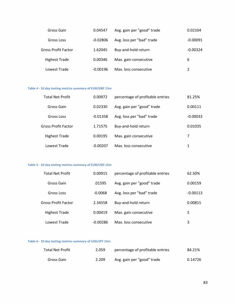
83
Gross Gain 0.04547 Avg. gain per "good" trade 0.02104
Gross Loss -0.02806 Avg. loss per "bad" trade -0.00091
Gross Profit Factor 1.62045 Buy-and-hold return -0.00324
Highest Trade 0.00346 Max. gain consecutive 6
Lowest Trade -0.00196 Max. loss consecutive 2
Table 4 - 10 day testing metrics summary of EUR/GBP 15m
Total Net Profit 0.00972 percentage of profitable entries 81.25%
Gross Gain 0.02330 Avg. gain per "good" trade 0.00111
Gross Loss -0.01358 Avg. loss per "bad" trade -0.00033
Gross Profit Factor 1.71575 Buy-and-hold return 0.01035
Highest Trade 0.00195 Max. gain consecutive 7
Lowest Trade -0.00207 Max. loss consecutive 1
Table 5 - 10 day testing metrics summary of EUR/USD 15m
Total Net Profit 0.00915 percentage of profitable entries 62.50%
Gross Gain .01595 Avg. gain per "good" trade 0.00159
Gross Loss -0.0068 Avg. loss per "bad" trade -0.00113
Gross Profit Factor 2.34558 Buy-and-hold return 0.00815
Highest Trade 0.00419 Max. gain consecutive 5
Lowest Trade -0.00286 Max. loss consecutive 3
Table 6 - 10 day testing metrics summary of USD/JPY 15m
Total Net Profit 2.059 percentage of profitable entries 84.21%
Gross Gain 2.209 Avg. gain per "good" trade 0.14726
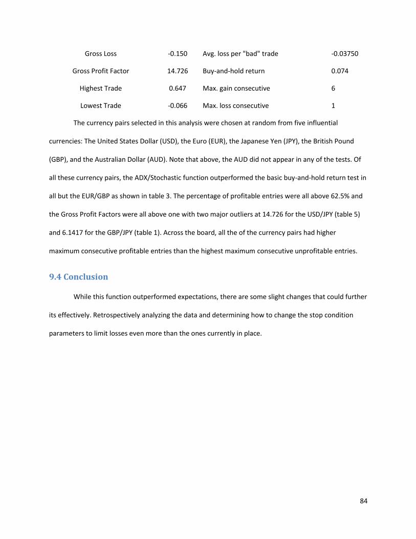
84
Gross Loss -0.150 Avg. loss per "bad" trade -0.03750
Gross Profit Factor 14.726 Buy-and-hold return 0.074
Highest Trade 0.647 Max. gain consecutive 6
Lowest Trade -0.066 Max. loss consecutive 1
The currency pairs selected in this analysis were chosen at random from five influential
currencies: The United States Dollar (USD), the Euro (EUR), the Japanese Yen (JPY), the British Pound
(GBP), and the Australian Dollar (AUD). Note that above, the AUD did not appear in any of the tests. Of
all these currency pairs, the ADX/Stochastic function outperformed the basic buy-and-hold return test in
all but the EUR/GBP as shown in table 3. The percentage of profitable entries were all above 62.5% and
the Gross Profit Factors were all above one with two major outliers at 14.726 for the USD/JPY (table 5)
and 6.1417 for the GBP/JPY (table 1). Across the board, all the of the currency pairs had higher
maximum consecutive profitable entries than the highest maximum consecutive unprofitable entries.
9.4 Conclusion
While this function outperformed expectations, there are some slight changes that could further
its effectively. Retrospectively analyzing the data and determining how to change the stop condition
parameters to limit losses even more than the ones currently in place.

85
10. Portfolio Algorithm Because the portfolio investment of different ratio can cause the different risk-return carves
among all the 38 currency ratios. In this cast, we can come up with the idea using Risk-free Asset, using
different division of the investment to get the best investment choice.
Figure 18: Choice of optimal portfolio combinations on the CML (Capital Marketing Line)
We use the theory of asset pricing models in Investment Analysis Portfolio Management by
Frank Reilly Keith Brown, and apply it to the currency ratio analysis.
Two rations analyze
How to choose the rations?
Based on the research we did in B term, referring to we came up the conclusion about the high
correlations about two different ratios. For example, for NZD/CAD, AUD/CAD has the highest
correlation, 0.835953 among other ratios; For EUR/GPY, AUD/JPY has the highest correlation, 0.970973,
compare others; and for AUD/USD and EUR/AUD, they have the highest correlation, 0.997838, among
all those ratios.

86
So I used the different sets of data to compare.
All the data are based on the close price. All the data calculated as following:
Average: average of all the close price of audjpy, eurjpy
Risk: variance of all the close price of audjpy, eurjpy
Cov: the covariance of all the close price of audjpy and eurjpy
Corr: the correlation of all the close price of audjpy and eurjpy.
W1 and W2: the sum of W1 and W2 =1, each number changes by 0.1

87
E(HPY): the ratio(W1 or W2) * related average return.
Expected variance for a two asset portfolio: ((x1^2)*v1) + (x2^2)*v2) + 2*x1*x2*c12
Standard (RFR)= (((x1^2)*v1) + (x2^2)*v2) + 2*x1*x2*c12)^0.5;
Min: minimum number of expected variance for a two-asset portfolio
Expected return=(E(HPY)-expected return of the year/360/24)/expected variance for a two asset
portfolio(risks) ( in this case, the expected return is 7%)
Max: maximum value of Expected return
CML: the line of capital market line based on the above analysis.Based on the research I
mentioned above, we can use this method further more. Instead, . I apply the portfolio
algorithm on the same data stream instead of portfolio management. Also I made some
implement on it. Instead of focusing on 5 bars if the historical data, I also apply it to 3 bars. The
basic strategy is
If weight_store_3 cross above weight_store_5 then
Buy next bar at open;
If weight_store_5 cross above weight_store_3 then
Sellshort next bar at open;
88
11. Historical Data Analysis:
As an investor, there are many strategies to employ to make investment decisions such as using
a specific technical indicator, Average True Range for example. Whatever the strategy may be, relevant
information must be provided in such a way so that it will ultimately lead to a profit. Our goal was to do
a pure technical analysis on the useful historical price data of the foreign exchange currencies through
TradeStation, disregarding any fundamental data. Although fundamental analysis techniques are
needed in the decision-making process, technical data and analysis was our main focus.
An important piece of technical data is when the market is active, or the activity time of the
market. By using TradeStation’s large collection of historical data as a means of data collection, we can
use the data to create further analyses and find out when the best times to enter or exit are for a given
ratio. Since the data is purely historical, the investor’s intuition based on current new events and other
such fundamental data will obviously still affect the trade decision.
Another important aspect when using historical data, is finding the correlation among all the
currency ratios. Finding similar trends among ratios could provide a basis on when to trade and also
some insight on when a trend is ending or beginning.
11.1 Method We used TradeStation to collect data for the open, close, high, and low prices for three scopes:
monthly, daily and hourly. We calculated the body range and the wick range for each time interval
(Figure 1) for each ratio in order to analyze the correlation and price activity, which will be helpful for
strategy implementation.

89
For example, to find the hourly price data for the Australian Dollar and the Canadian Dollar,
AUD/CAD, we exported data from the TradeStation Data Window through Chart Analysis into a text
document. From there, it was converted to an Excel spreadsheet so that further analysis could be done .
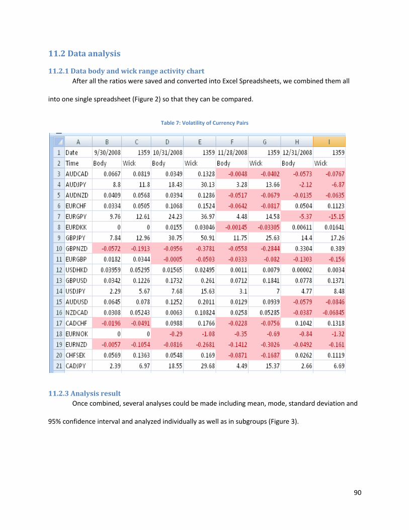
90
11.2 Data analysis
11.2.1 Data body and wick range activity chart
After all the ratios were saved and converted into Excel Spreadsheets, we combined them all
into one single spreadsheet (Figure 2) so that they can be compared.
Table 7: Volatility of Currency Pairs
11.2.3 Analysis result
Once combined, several analyses could be made including mean, mode, standard deviation and
95% confidence interval and analyzed individually as well as in subgroups (Figure 3).

91
11.2.4 Correlation
Using this data, we were able to find out the best times to trade using a series of calculations.
With the data available on TradeStation now converted into Excel spreadsheets, we went through the
following process for each ratio:
First, we standardized the body and wick ranges for the ratio so that we could compare them to
the body and wick ranges for the other ratios. Next, we took the average values of the per day body and
wick range averages for monthly data or per hour body and wick range averages for daily data and
found the standardized averages per day and per hour for daily and monthly data respectively. Refer to
the Evaluation of Data section for results.
We also calculated the correlation among each of the ratios, which shows how similar one
currency ratio is to another historically. We used monthly data when finding these correlations to find a
more general trend with the mentality that as the time interval becomes smaller and smaller, the
correlation among the ratios will have less of a deciding factor.
Table 8: Confidence Intervals of Currency Pairs (Appendix 9)

92
11.3 Evaluation of Data There are trends that can be seen from the data we have collected. Most notable is the daily
activity chart for wick ranges. There is a definite general trend for times when active trading is
occurring. For example, the chart below illustrates the activity for currency ratios that include the US
Dollar or the Canadian Dollar. The active times of most of these ratios are around 2 AM, 9 AM, and 7
PM Eastern Standard Time according to our data. See Appendices for more results.
Figure 19 - Normalized Average Currency Pair Activity
-1.5
-1
-0.5
0
0.5
1
1.5
1 2 3 4 5 6 7 8 9 10 11 12 13 14 15 16 17 18 19 20 21 22 23 24
No
rmal
ize
d w
ick
ran
ge a
vera
ges
by
ho
ur
Time of Day
Activity Chart (Ratios including USD, CAD)
AUDUSD
CADCHF
CADJPY
EURCAD
EURUSD
GBPCAD
GBPUSD
NZDCAD
NZDUSD
USDCAD
USDCHF
USDDKK
USDHKD
USDJPY

93
12. Active Time Analysis
First get the body and wick range use close-open and high- low. And in order to compare data
with all the ratios, we standardize the all the ratios with the average of wick range and body range.
We used the normalized value which has been stand zed by the mean and standard derivation in this
way , it possible to be efficiently compared against other values.
Interval activity period explanation
According to the data we got from Tradestation, I use the hourly and the daily data as the
reference. The reason is the hourly data is more valuable for the activity time research. Also, the day of
week can also help because according to people’s psychology.
Body or Wick?
At first I did the research on the wick range. In this case, the research we get can be used for
activity period. And then I use the body change, which is the close price minus the previous day close
price. In this case we can not only get the activity period for trading, which ratio is more valuable but
also, which time interval has more chance to get profit.
Directly compare & STANDARDIZE
Because the spread of the different ratios is different, so it would hard to compare between
different ratios. So I use the STANDARDIZE function, which can compare the different current ratios at
the same time.
Final Result

94
Day of Week:
Figure 20: Currency Volatilities by Day
Combine all the ratios, we find on Tuesday and Friday, forex market is very active, and for the wick, we
can see Thursday Trading can get more profit
Hour of the day
Figure 21: Currency Volatilities by Hour
According to the data, we divide them into big wave activity time and small wave activity time.
During the big wave activity period, the forex market gets more active than the small wave activity. The
big waves are: 2am, 7-9am, and 5pm. The small Wave is 1pm.
-0.15
-0.1
-0.05
0
0.05
0.1
-2.08
-2.06
-2.04
-2.02
-2
-1.98
-1.96
-1.94
-1.92
Mon Tue Wed Thur Fri
Body
Wick
0
0.01
0.02
0.03
0.04
0.05
0.06
0.07
-0.15
-0.1
-0.05
0
0.05
0.1
0.15
1 2 3 4 5 6 7 8 9 10 11 12 13 14 15 16 17 18 19 20 21 22 23 24
Body
Wick
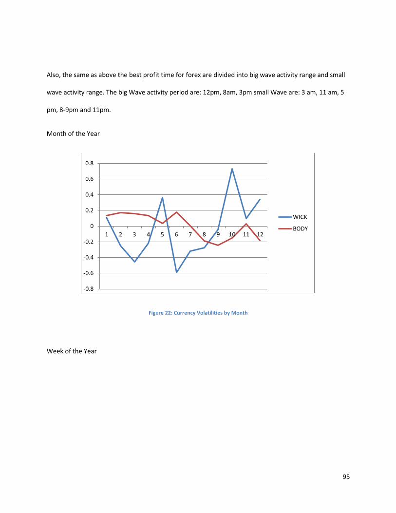
95
Also, the same as above the best profit time for forex are divided into big wave activity range and small
wave activity range. The big Wave activity period are: 12pm, 8am, 3pm small Wave are: 3 am, 11 am, 5
pm, 8-9pm and 11pm.
Month of the Year
Figure 22: Currency Volatilities by Month
Week of the Year
-0.8
-0.6
-0.4
-0.2
0
0.2
0.4
0.6
0.8
1 2 3 4 5 6 7 8 9 10 11 12
WICK
BODY
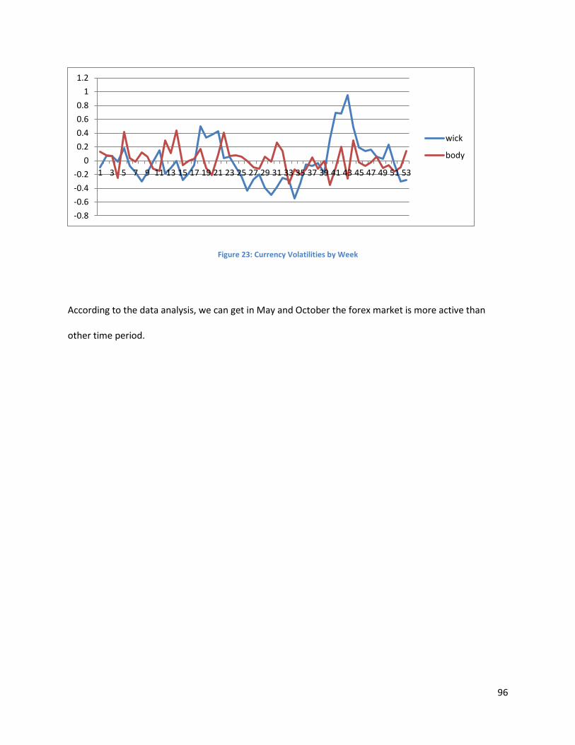
96
Figure 23: Currency Volatilities by Week
According to the data analysis, we can get in May and October the forex market is more active than
other time period.
-0.8
-0.6
-0.4
-0.2
0
0.2
0.4
0.6
0.8
1
1.2
1 3 5 7 9 11 13 15 17 19 21 23 25 27 29 31 33 35 37 39 41 43 45 47 49 51 53
wick
body
97
13. Live Trading Up to this point our discussion of trading has been based solely upon analyzing how our
algorithms performed on historical data. While this testing is vital to developing and testing successful
strategies, it does not provide the complete experience of trading. In fact, there are quite a few
significant differences that make it so that a strategy developed through historical testing will not
necessarily be profitable when used for actual trading. We will exam each of these disparities so that we
can determine how to accommodate for them in transitioning from historical to live strategy
applications.
13.1 Bid and Ask Prices As discussed in the background section, the actual exchanging of stocks revolves around market
makers. These market makers are performing a service for traders by facilitating the exchange process,
so of course they must be paid. The way in which market makers are able to profit is by including a
commission in the price that they are buying and selling stocks at. The commission adjusted asset prices
are called the bid and ask prices, and are the actual prices that are applied to traders. The bid price is
the price at which the market maker will buy a security, and the ask price is the price that the market
maker will sell a security for. To ensure that a profit is made, the bid price is always less than or equal to
the asset price, and the ask price is always greater than or equal to the asset price. Bid and ask prices are
constantly fluctuating and can be very inconsistent, so they are generally not included in historical data,
which is the case in Tradestation. This means that strategies tested on historical data do not account for
the market maker commission, so profits are exaggerated.
One could just simply acknowledge that profits made from real trading are strictly less than
those from historical trading and move on, but more consideration should be given to developing
strategies that can account for the adjusted prices. First of all, it should be noted that a trader that
doesn’t trade frequently, but holds positions for long periods of time will be less affected by the

98
commission than a trader who trades frequently for smaller profits. More simply put, less trades means
less commissions, but profits are not necessarily altered. As a result, we should favor longer term
trading strategies when moving to live trading. Another improvement that could be made to our
algorithms would be to check the bid and ask prices of assets before opening positions, and avoiding
investments when the market maker commission is too high. Finally, some comprehensive analysis
should be done to find a relationship between the bid and ask prices and asset price movement to see if
they can be helpful in predicting price movements.
13.2 Intra Bar Data A benefit to live trading over historical data analysis is that the trader is able to watch the asset
price move within the current bar. Historical plots only display four points that are achieved in each bar,
but live trading displays all of them. The additional information provides traders with a much stronger
basis for predicting trends in the stock price on a shorter term basis, so it could be very helpful in our
algorithms. Unfortunately, this turns out to be another advantage to manual rather than automated
trading, because Tradestation does not offer any functionality for constant price data analysis in real
time. We expect future development in automated trading systems to correct this issue, but for now we
must simply work around it.
13.3 Constant Operation In the United States, the normal trading day starts at 9:30 AM and ends at 4:00 PM, a total
period of six and a half hours. It is difficult for any one person to constantly be watching stock charts for
this entire period of time without taking a break, while a computer doesn’t have that problem. One
issue that does arise is that leaving a computer running unattended for that long of a time can be
hazardous. Computers can overheat, automatically restart for updates, the power can go out, internet
can go down, and many other things can occur. If any of these things were to happen while the
computer has an open position, it can lead to a large loss. As a result we note that automated trading
99
strategies are not perfectly self-sufficient, as they do require some monitoring to make sure they
haven’t been shut down for some reason.
13.4 Results We used the IMT to perform some live trading and see how well it could perform in the actual
trading environment. The algorithm was applied to ten stocks: AAPL, BIDU, PFE, MS, MSFT, RIMM,
GOOG, AMZN, EBAY, and VZ. We did some monitoring of the algorithm while it was performing live
trading, but it was allowed to make all of its own decisions on trades without any personal intervention.
In its trading the algorithm encountered the .01$ per share commission cost, real bid and ask prices
following the stocks in real time. When a buy signal was triggered, the algorithm would buy one share of
the given stock.
The results in general were good and the algorithm was profitable every day that it was applied.
On each day of trading, there were between zero and three trades generated, and over the testing
period only one trade yielded a loss. The average profit per day was about $2, and we would not have
needed to invest any money to be able to perform the trades with a margin trading account.
One issue encountered was a lack of aggressiveness by the algorithm, in that it did not make
very many trades. In terms of managing the risk of our investment this is a good thing however,
especially with an unmonitored automated trading strategy. We were fortunate in our testing that due
to the nature of our algorithm, it did not spend a large amount of time with open trades, so on a few
occasions where we temporarily lost internet access, we didn’t have any open positions anyways. A
comprehensive analysis of live trading results can be found in the appendix.

100
14. Conclusion Overall we can say that the work done here was a great success. We successfully achieved our
goal of developing an algorithm that can run by itself and make decisions with minimal risk that
profitably trade assets. It took a great deal of research and patience to get to this point, which is
understandable because so many people try and fail at determining how to invest profitably. While our
primary goal was achieved however, there are areas in which further work could be done on this topic.
14.1 Future Work First of all, our work found an algorithm to successfully trade on an intraday time frame. This is
useful for our purposes, but for some it requires too much time commitment. Many traders are very
busy and do not wish to have to monitor their investments every day, so they opt to partake in longer
term investments. As a result, in the future we hope to be able to look more at developing long term
trading strategies that involve a minimal amount of market monitoring.
In each of our algorithms, we mainly focused on trading in one particular bar interval. An
interesting question however, would be to determine which bar intervals are the best to trade on. The
word “best” here could mean many things, such as most profitable, easiest to use, or requires the least
work, but some sort of comprehensive analysis of the different trading intervals would be very useful to
traders.
14.2 Suggestions It is our hope that the work done here can be used to help people that also hope to develop
automated techniques for investment. Our experiences in learning about asset trading and the
programming methods involved in it has provided a great body of knowledge that can be helpful to
beginner traders.
The first recommendation we can offer is to start watching live chart movements early and
often. While watching charts begin to decide when to buy, short, and close positions. So many traders

101
are successful because they have spent so much time watching the markets and have learned the
common patterns it follows. Therefore, it is essential for beginners to start trying to identify patterns
right away, because being able to see where patterns emerge is the key to successful trading.
A major mistake traders often make is to use technical indicators without understanding how
they work. It is so tempting to rely heavily on indicator data because it seems so simply to just buy or
sell when they provide such a signal. Unfortunately, trading is not that easy. The only way to be able to
effectively use indicators is by having a deeper understanding of the way each indicator is calculated and
where it does and doesn’t work. It cannot be overstated how important it is to know exactly what an
indicator is saying.
When using automated trading strategies, one is placing a large amount of faith in the
algorithms to not make mistakes. To be able to have such faith requires a great deal of testing and
analysis of the algorithm. The slightest mistakes in an algorithm can still cause major problems in actual
trading, so they need to be ironed out long before one should ever trade with an algorithm. With the
right degree of testing and preparation however, automated trading strategies can be very profitable.
102
15. References
Works Cited Acceleration Bands. (n.d.). Retrieved October 5, 2010, from Forex Indicators: http://forex-
indicators.net/acceleration-bands
Average Directional Index (ADX). (1999). Retrieved November 30, 2010, from Chart School:
http://stockcharts.com/help/doku.php?id=chart_school:technical_indicators:average_directional_
Average True Range. (n.d.). Retrieved October 8, 2010, from MQL4 Technical Analysis:
http://ta.mql4.com/indicators/oscillators/average_true_range
Bar Charts (OHLC). (n.d.). Retrieved 10 8, 2010, from Incrediblecharts:
http://www.incrediblecharts.com/technical/bar_charts.php
Candlestick. (n.d.). Retrieved 11 13, 2010, from Investopedia:
http://www.investopedia.com/terms/c/candlestick.asp
Deaton, M. (2008). Fibonacci Retracements. Retrieved October 27, 2010, from Fibonacci Genious:
http://www.fibonaccigenius.com/fibonacci-retracements.html
Elder Ray Bull and Bear Power. (2010). Retrieved December 7, 2010, from Free Stock Charts:
http://www.freestockcharts.com/Help/Content/Indicators/Elder%20Ray%20Bull%20and%20Bear%20Po
wer.htm
Elliot Wave Theory. (n.d.). Retrieved September 15, 2010, from Acrotec:
http://www.acrotec.com/ewt.htm
Guevara, A. (2010, December 14). Tradestation Labs. Retrieved January 29, 2011, from Tradestation:
https://www.tradestation.com/support/tslabs/default.aspx?report=14
Haines, S. (2004, November 18). Price Volume Chart. Retrieved from InformIt:
http://www.informit.com/guides/content.aspx?g=java&seqNum=76
Introduction. (n.d.). Retrieved September 15, 2010, from Bollinger Bands:
http://www.bollingerbands.com/services/bb/
Jepsen, L. (n.d.). Use The Stochastic Oscillator Wrong And Stay Poor Or Use It Right And Become Rich.
Retrieved October 29, 2010, from Guerilla Stock Trading:
http://www.guerillastocktrading.com/technical-analysis/use-the-stochastic-oscillator-wrong-and-stay-
poor-or-use-it-right-and-become-rich
Moving Average Convergence Divergence (MACD). (2006). Retrieved September 9, 2010, from Yahoo!
Finance: http://biz.yahoo.com/charts/guide15.html

103
Relative Strength Index. (2007). Retrieved September 18, 2010, from Online Trading Concepts:
http://www.onlinetradingconcepts.com/TechnicalAnalysis/RelativeStrengthIndex.html
Townsend, J. (2010, August 5). True Strength Index (TSI) - Settings and Techniques. Retrieved December
5, 2010, from Daily Markets: http://www.dailymarkets.com/stock/2010/08/05/true-strength-index-tsi-
settings-and-techniques/
Ultimate Oscillator. (n.d.). Retrieved December 9, 2010, from Forex Realm:
http://www.forexrealm.com/technical-analysis/technical-indicators/ultimate-oscillator.html
Using the Ichimoku Cloud. (2007). Retrieved November 28, 2010, from FX Words:
http://www.fxwords.com/u/ichimoku-cloud.html
Yu-Hon Lui, David Mole. use of fundamental and technical analyses. Hong Kong: Journal of International
Money and Finance.
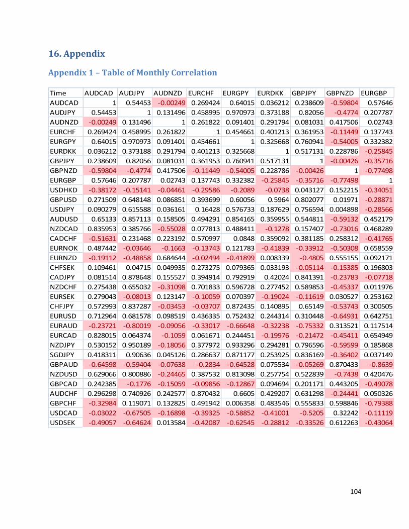
104
16. Appendix
Appendix 1 – Table of Monthly Correlation
Time AUDCAD AUDJPY AUDNZD EURCHF EURGPY EURDKK GBPJPY GBPNZD EURGBP
AUDCAD 1 0.54453 -0.00249 0.269424 0.64015 0.036212 0.238609 -0.59804 0.57646
AUDJPY 0.54453 1 0.131496 0.458995 0.970973 0.373188 0.82056 -0.4774 0.207787
AUDNZD -0.00249 0.131496 1 0.261822 0.091401 0.291794 0.081031 0.417506 0.02743
EURCHF 0.269424 0.458995 0.261822 1 0.454661 0.401213 0.361953 -0.11449 0.137743
EURGPY 0.64015 0.970973 0.091401 0.454661 1 0.325668 0.760941 -0.54005 0.332382
EURDKK 0.036212 0.373188 0.291794 0.401213 0.325668 1 0.517131 0.228786 -0.25845
GBPJPY 0.238609 0.82056 0.081031 0.361953 0.760941 0.517131 1 -0.00426 -0.35716
GBPNZD -0.59804 -0.4774 0.417506 -0.11449 -0.54005 0.228786 -0.00426 1 -0.77498
EURGBP 0.57646 0.207787 0.02743 0.137743 0.332382 -0.25845 -0.35716 -0.77498 1
USDHKD -0.38172 -0.15141 -0.04461 -0.29586 -0.2089 -0.0738 0.043127 0.152215 -0.34051
GBPUSD 0.271509 0.648148 0.086851 0.393699 0.60056 0.5964 0.802077 0.01971 -0.28871
USDJPY 0.090279 0.615588 0.036161 0.16428 0.576733 0.187629 0.756594 0.004898 -0.28566
AUDUSD 0.65133 0.857113 0.158505 0.494291 0.854165 0.359955 0.544811 -0.59132 0.452179
NZDCAD 0.835953 0.385766 -0.55028 0.077813 0.488411 -0.1278 0.157407 -0.73016 0.468289
CADCHF -0.51631 0.231468 0.223192 0.570997 0.0848 0.359092 0.381185 0.258312 -0.41765
EURNOK 0.487442 -0.03646 -0.1663 -0.13743 0.121783 -0.41839 -0.33912 -0.50308 0.658559
EURNZD -0.19112 -0.48858 0.684644 -0.02494 -0.41899 0.008339 -0.4805 0.555155 0.092171
CHFSEK 0.109461 0.04715 0.049935 0.273275 0.079365 0.033193 -0.05114 -0.15385 0.196803
CADJPY 0.081514 0.878648 0.155527 0.394914 0.792919 0.42024 0.841391 -0.23783 -0.07718
NZDCHF 0.275438 0.655032 -0.31098 0.701833 0.596728 0.277452 0.589853 -0.45337 0.011976
EURSEK 0.279043 -0.08013 0.123147 -0.10059 0.070397 -0.19024 -0.11619 0.030527 0.253162
CHFJPY 0.572993 0.837287 -0.03453 -0.03707 0.872435 0.140895 0.65149 -0.53743 0.300505
EURUSD 0.712964 0.681578 0.098519 0.436335 0.752432 0.244314 0.310448 -0.64931 0.642751
EURAUD -0.23721 -0.80019 -0.09056 -0.33017 -0.66648 -0.32238 -0.75332 0.313521 0.117514
EURCAD 0.828015 0.064374 -0.1059 0.061671 0.244451 -0.19976 -0.21472 -0.45411 0.654949
NZDJPY 0.530152 0.950189 -0.18056 0.377972 0.933296 0.294281 0.796596 -0.59599 0.185868
SGDJPY 0.418311 0.90636 0.045126 0.286637 0.871177 0.253925 0.836169 -0.36402 0.037149
GBPAUD -0.64598 -0.59404 -0.07638 -0.2834 -0.64528 0.075534 -0.05269 0.870433 -0.8639
NZDUSD 0.629066 0.800886 -0.24465 0.387532 0.813098 0.257754 0.522839 -0.7438 0.420476
GBPCAD 0.242385 -0.1776 -0.15059 -0.09856 -0.12867 0.094694 0.201171 0.443205 -0.49078
AUDCHF 0.296298 0.740926 0.242577 0.870432 0.6605 0.429207 0.631298 -0.24441 0.050326
GBPCHF -0.32984 0.119071 0.132825 0.491942 0.006358 0.483546 0.555833 0.598846 -0.79388
USDCAD -0.03022 -0.67505 -0.16898 -0.39325 -0.58852 -0.41001 -0.5205 0.32242 -0.11119
USDSEK -0.49057 -0.64624 0.013584 -0.42087 -0.62545 -0.28812 -0.33526 0.612263 -0.43064
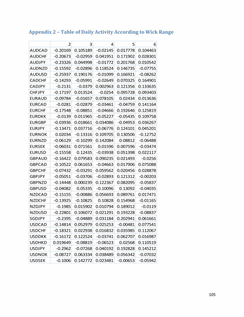
105
Appendix 2 – Table of Daily Activity According to Wick Range
2 3 4 5 6
AUDCAD -0.20169 0.105189 -0.02145 0.017778 0.104463
AUDCHF -0.20673 -0.02959 0.041951 0.171902 0.028301
AUDJPY -0.23326 0.044998 -0.01772 0.201768 0.010542
AUDNZD -0.15592 -0.02896 0.118524 0.146735 -0.07755
AUDUSD -0.25937 0.190176 -0.01099 0.166921 -0.08262
CADCHF -0.14293 -0.05991 -0.02649 0.070325 0.164901
CADJPY -0.2131 -0.0379 0.002963 0.121356 0.133635
CHFJPY -0.17197 0.013524 -0.0254 0.095728 0.093403
EURAUD -0.09784 -0.01657 0.078105 0.02434 0.013636
EURCAD -0.0281 -0.02879 -0.03461 -0.04759 0.141164
EURCHF -0.17548 -0.08851 -0.04666 0.192646 0.125819
EURDKK -0.0139 0.011965 -0.05227 -0.05435 0.109758
EURGBP -0.03936 0.018661 0.034086 -0.04953 0.036267
EURJPY -0.13471 0.037716 -0.06776 0.124101 0.045201
EURNOK 0.02034 -0.13316 0.109705 0.130506 -0.12752
EURNZD -0.06129 -0.10299 0.142084 0.08812 -0.06488
EURSEK -0.06031 0.071561 0.01596 0.007596 -0.03474
EURUSD -0.15558 0.12435 -0.03938 0.051398 0.022117
GBPAUD -0.16422 0.079583 0.090235 0.021493 -0.0256
GBPCAD -0.10522 0.061653 -0.04663 0.017906 0.075088
GBPCHF -0.07432 -0.03291 0.059562 0.020456 0.028878
GBPJPY -0.05051 -0.03706 -0.02893 0.121312 -0.00203
GBPNZD -0.14448 0.000239 0.122367 0.082095 -0.05837
GBPUSD -0.04082 0.05335 -0.10096 0.13092 -0.04035
NZDCAD -0.15155 -0.00886 0.056693 0.089761 0.017471
NZDCHF -0.13925 -0.10825 0.10828 0.154968 -0.01165
NZDJPY -0.1985 0.015902 0.010794 0.189012 -0.0119
NZDUSD -0.22801 0.106072 0.021291 0.193228 -0.08837
SGDJPY -0.2395 -0.04889 0.031184 0.202941 0.061661
USDCAD -0.14814 0.052979 0.025253 -0.00481 0.077541
USDCHF -0.18321 0.022938 0.016832 0.035985 0.112067
USDDKK -0.16172 0.122524 -0.03741 0.062707 0.016987
USDHKD 0.019649 -0.08819 -0.06523 0.02568 0.110519
USDJPY -0.2962 -0.07268 0.040192 0.192828 0.145212
USDNOK -0.08727 0.063334 0.038489 0.056342 -0.07032
USDSEK -0.1006 0.142772 0.023481 -0.00653 -0.05942
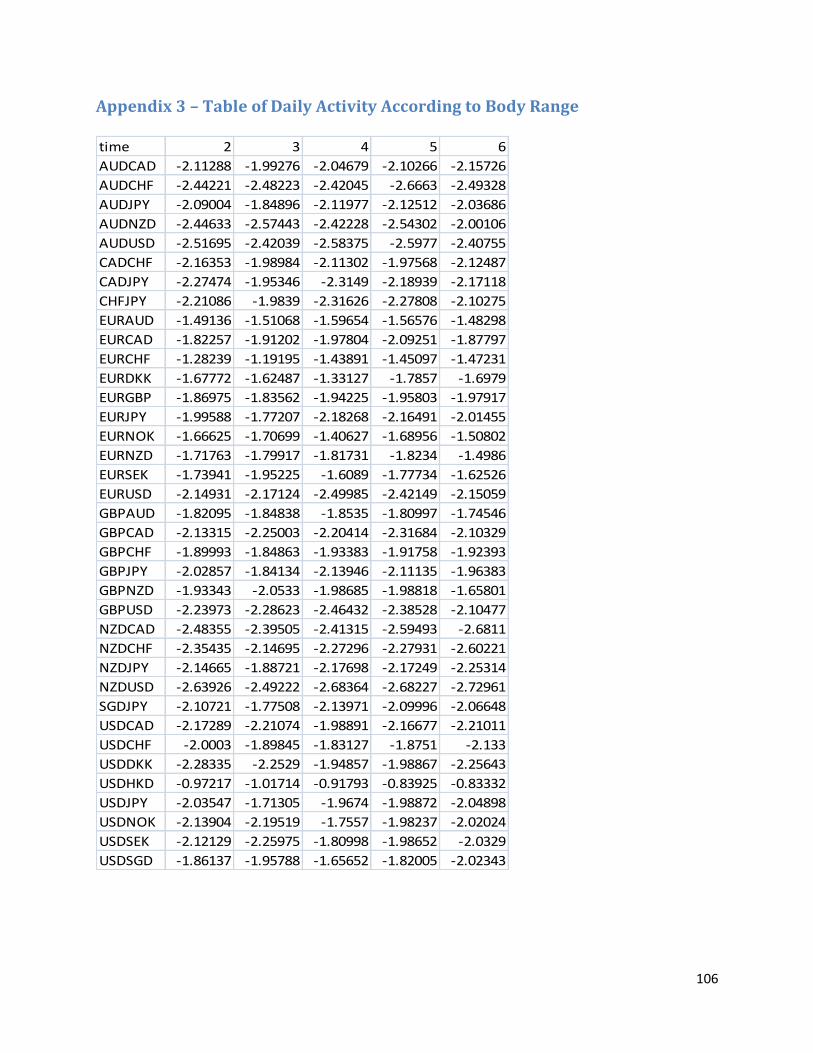
106
Appendix 3 – Table of Daily Activity According to Body Range
time 2 3 4 5 6
AUDCAD -2.11288 -1.99276 -2.04679 -2.10266 -2.15726
AUDCHF -2.44221 -2.48223 -2.42045 -2.6663 -2.49328
AUDJPY -2.09004 -1.84896 -2.11977 -2.12512 -2.03686
AUDNZD -2.44633 -2.57443 -2.42228 -2.54302 -2.00106
AUDUSD -2.51695 -2.42039 -2.58375 -2.5977 -2.40755
CADCHF -2.16353 -1.98984 -2.11302 -1.97568 -2.12487
CADJPY -2.27474 -1.95346 -2.3149 -2.18939 -2.17118
CHFJPY -2.21086 -1.9839 -2.31626 -2.27808 -2.10275
EURAUD -1.49136 -1.51068 -1.59654 -1.56576 -1.48298
EURCAD -1.82257 -1.91202 -1.97804 -2.09251 -1.87797
EURCHF -1.28239 -1.19195 -1.43891 -1.45097 -1.47231
EURDKK -1.67772 -1.62487 -1.33127 -1.7857 -1.6979
EURGBP -1.86975 -1.83562 -1.94225 -1.95803 -1.97917
EURJPY -1.99588 -1.77207 -2.18268 -2.16491 -2.01455
EURNOK -1.66625 -1.70699 -1.40627 -1.68956 -1.50802
EURNZD -1.71763 -1.79917 -1.81731 -1.8234 -1.4986
EURSEK -1.73941 -1.95225 -1.6089 -1.77734 -1.62526
EURUSD -2.14931 -2.17124 -2.49985 -2.42149 -2.15059
GBPAUD -1.82095 -1.84838 -1.8535 -1.80997 -1.74546
GBPCAD -2.13315 -2.25003 -2.20414 -2.31684 -2.10329
GBPCHF -1.89993 -1.84863 -1.93383 -1.91758 -1.92393
GBPJPY -2.02857 -1.84134 -2.13946 -2.11135 -1.96383
GBPNZD -1.93343 -2.0533 -1.98685 -1.98818 -1.65801
GBPUSD -2.23973 -2.28623 -2.46432 -2.38528 -2.10477
NZDCAD -2.48355 -2.39505 -2.41315 -2.59493 -2.6811
NZDCHF -2.35435 -2.14695 -2.27296 -2.27931 -2.60221
NZDJPY -2.14665 -1.88721 -2.17698 -2.17249 -2.25314
NZDUSD -2.63926 -2.49222 -2.68364 -2.68227 -2.72961
SGDJPY -2.10721 -1.77508 -2.13971 -2.09996 -2.06648
USDCAD -2.17289 -2.21074 -1.98891 -2.16677 -2.21011
USDCHF -2.0003 -1.89845 -1.83127 -1.8751 -2.133
USDDKK -2.28335 -2.2529 -1.94857 -1.98867 -2.25643
USDHKD -0.97217 -1.01714 -0.91793 -0.83925 -0.83332
USDJPY -2.03547 -1.71305 -1.9674 -1.98872 -2.04898
USDNOK -2.13904 -2.19519 -1.7557 -1.98237 -2.02024
USDSEK -2.12129 -2.25975 -1.80998 -1.98652 -2.0329
USDSGD -1.86137 -1.95788 -1.65652 -1.82005 -2.02343

107
Appendix 4– Table of Monthly Body and Wick Ranges
Date Time AUDCAD AUDJPY AUDNZD EURCHF EURGPY EURDKK GBPJPY GBPNZD
9/30/2008 Body 0.0667 8.8 0.0409 0.0334 9.76 0 7.84 -0.0572
1359 Wick 0.0819 11.8 0.0568 0.0505 12.61 0 12.96 -0.1913
10/31/2008 Body 0.0349 18.43 0.0394 0.1068 24.23 0.0155 30.75 -0.0956
1359 Wick 0.1328 30.13 0.1286 0.1524 36.97 0.03046 50.91 -0.3781
11/28/2008 Body -0.0048 3.28 -0.0517 -0.0642 4.48 -0.00145 11.75 -0.0558
1359 Wick -0.0402 13.66 -0.0679 -0.0817 14.58 -0.03305 25.63 -0.2844
12/31/2008 Body -0.0573 -2.12 -0.0135 0.0504 -5.37 0.00611 14.4 0.3304
1359 Wick -0.0767 -6.87 -0.0635 0.1123 -15.15 0.01641 17.26 0.389
1/30/2009 Body 0.0686 6.18 -0.0472 0.0035 11.02 -0.00757 2.46 -0.3263
1359 Wick 0.0909 12.02 -0.1055 0.0535 16.47 -0.00873 22.7 -0.4116
2/27/2009 Body -0.0335 -5.07 -0.0246 0.0026 -8.69 0.0025 -9.44 -0.0155
1359 Wick -0.0639 -9.03 -0.0398 0.045 -12.94 0.00604 -16.46 -0.1616
3/31/2009 Body -0.0548 -5.94 0.0447 -0.0305 -7.68 0.00224 -2.03 0.3025
1359 Wick -0.074 -8.61 0.0881 -0.0869 -12.78 0.01024 -13.64 0.4013
4/30/2009 Body 0.0062 -3.16 -0.0483 0.0013 0.61 -0.00084 -4.17 -0.0573
1359 Wick 0.0387 -6.66 -0.0895 0.0285 13.04 -0.00722 -12.5 -0.1592
5/29/2009 Body -0.0081 -4.81 0.0324 -0.0023 -4.5 0.00123 -8.42 0.0836
1359 Wick -0.035 -6.39 0.0447 -0.0229 -8.72 0.00824 -12.72 0.1432
6/30/2009 Body -0.0605 -1.19 0.0052 -0.0156 -0.62 -0.00098 -4.45 -0.023
1359 Wick -0.0673 -6.4 0.0444 -0.0373 -7.8 -0.00587 -9.09 -0.1069
7/31/2009 Body 0.0371 -1.41 -0.0147 0.0012 0.28 0.00017 0.44 0.0237
1359 Wick 0.0592 -8.71 -0.035 0.0237 9.87 0.00549 13.23 0.1247
8/31/2009 Body -0.0233 0.62 0.0341 0.0058 1.74 0.00377 6.8 0.1551
1359 Wick -0.0324 5.32 0.054 0.0229 6.58 0.0056 13.05 0.1869
9/30/2009 Body -0.0212 -0.63 0.0103 0.0011 2.12 -0.00172 8.27 0.1665
1359 Wick -0.0426 -3.65 0.0445 0.016 5.69 -0.00559 13.53 0.2279
10/30/2009 Body -0.0297 -1.77 -0.0301 0.0058 -1.39 0.00212 -4.83 -0.0793
1359 Wick -0.0503 -8.99 -0.0619 0.0122 -9.46 0.00312 -13.54 -0.167
11/30/2009 Body 0.0048 1.25 -0.0231 0.0013 2.35 0.00058 5.07 0.0009
1359 Wick 0.0347 7.66 -0.0379 0.0136 8.86 0.00453 12.34 0.0964
12/31/2009 Body 0.0224 -4.38 0.0397 0.0249 -3.68 0.00007 -8.44 0.0698
1359 Wick 0.06 -5.27 0.0519 0.032 -7.24 0.00463 -9.05 0.103
1/29/2010 Body -0.0009 3.77 -0.0192 0.0128 7.84 -0.00385 5.54 -0.0542
1359 Wick -0.0268 6.54 -0.0377 0.0253 9.58 -0.00662 7.07 -0.1382
2/26/2010 Body 0.0006 -0.38 -0.0265 0.0072 3.54 0.00305 7.86 0.094
1359 Wick 0.0248 -6.63 -0.0516 0.025 7.33 0.00386 10.64 0.1291
3/31/2010 Body 0.0137 -6.08 -0.0085 0.0391 -5.2 -0.00123 -7.25 0.0312
1359 Wick 0.0218 -6.65 -0.0322 0.0446 -6.81 -0.00615 -10.01 0.1044
4/30/2010 Body -0.0096 -0.98 0.0197 -0.009 1.5 0.00153 -1.46 0.0356
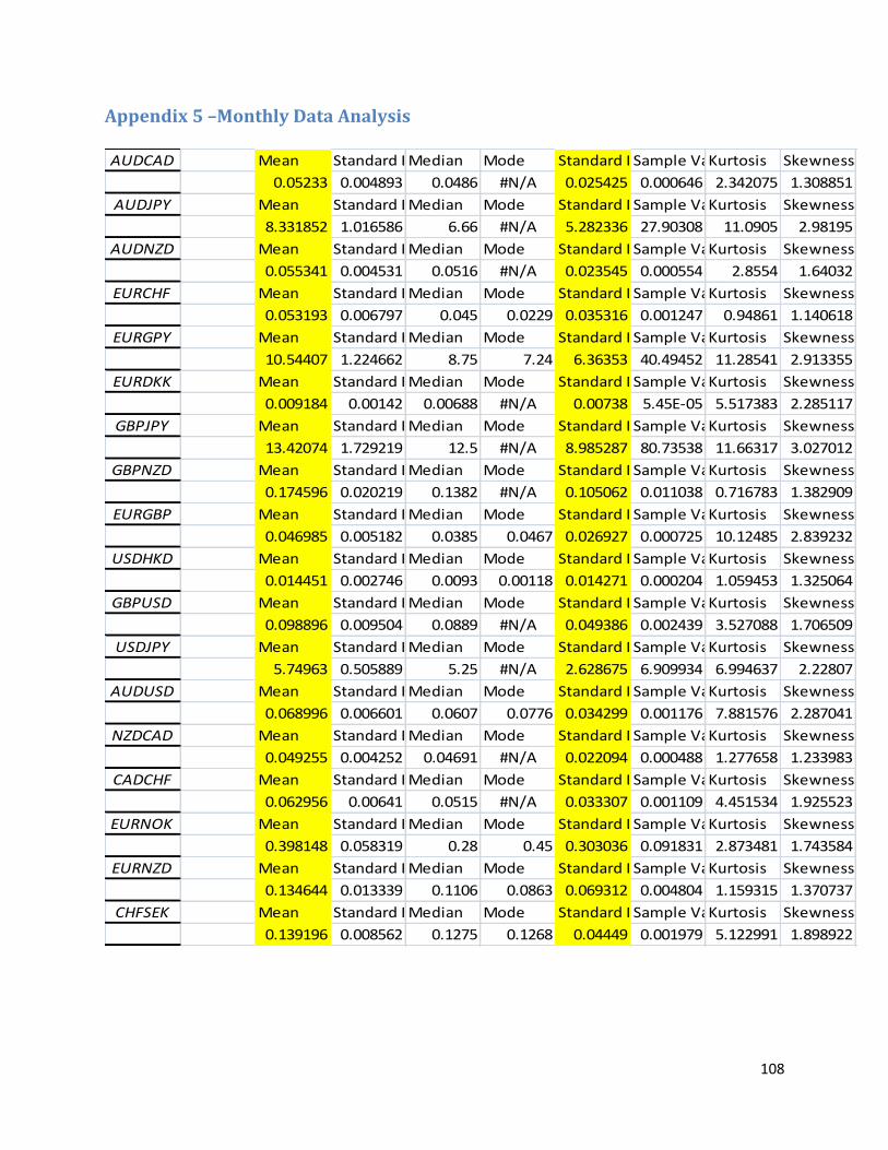
108
Appendix 5 –Monthly Data Analysis
AUDCAD Mean Standard ErrorMedian Mode Standard DeviationSample VarianceKurtosis Skewness
0.05233 0.004893 0.0486 #N/A 0.025425 0.000646 2.342075 1.308851
AUDJPY Mean Standard ErrorMedian Mode Standard DeviationSample VarianceKurtosis Skewness
8.331852 1.016586 6.66 #N/A 5.282336 27.90308 11.0905 2.98195
AUDNZD Mean Standard ErrorMedian Mode Standard DeviationSample VarianceKurtosis Skewness
0.055341 0.004531 0.0516 #N/A 0.023545 0.000554 2.8554 1.64032
EURCHF Mean Standard ErrorMedian Mode Standard DeviationSample VarianceKurtosis Skewness
0.053193 0.006797 0.045 0.0229 0.035316 0.001247 0.94861 1.140618
EURGPY Mean Standard ErrorMedian Mode Standard DeviationSample VarianceKurtosis Skewness
10.54407 1.224662 8.75 7.24 6.36353 40.49452 11.28541 2.913355
EURDKK Mean Standard ErrorMedian Mode Standard DeviationSample VarianceKurtosis Skewness
0.009184 0.00142 0.00688 #N/A 0.00738 5.45E-05 5.517383 2.285117
GBPJPY Mean Standard ErrorMedian Mode Standard DeviationSample VarianceKurtosis Skewness
13.42074 1.729219 12.5 #N/A 8.985287 80.73538 11.66317 3.027012
GBPNZD Mean Standard ErrorMedian Mode Standard DeviationSample VarianceKurtosis Skewness
0.174596 0.020219 0.1382 #N/A 0.105062 0.011038 0.716783 1.382909
EURGBP Mean Standard ErrorMedian Mode Standard DeviationSample VarianceKurtosis Skewness
0.046985 0.005182 0.0385 0.0467 0.026927 0.000725 10.12485 2.839232
USDHKD Mean Standard ErrorMedian Mode Standard DeviationSample VarianceKurtosis Skewness
0.014451 0.002746 0.0093 0.00118 0.014271 0.000204 1.059453 1.325064
GBPUSD Mean Standard ErrorMedian Mode Standard DeviationSample VarianceKurtosis Skewness
0.098896 0.009504 0.0889 #N/A 0.049386 0.002439 3.527088 1.706509
USDJPY Mean Standard ErrorMedian Mode Standard DeviationSample VarianceKurtosis Skewness
5.74963 0.505889 5.25 #N/A 2.628675 6.909934 6.994637 2.22807
AUDUSD Mean Standard ErrorMedian Mode Standard DeviationSample VarianceKurtosis Skewness
0.068996 0.006601 0.0607 0.0776 0.034299 0.001176 7.881576 2.287041
NZDCAD Mean Standard ErrorMedian Mode Standard DeviationSample VarianceKurtosis Skewness
0.049255 0.004252 0.04691 #N/A 0.022094 0.000488 1.277658 1.233983
CADCHF Mean Standard ErrorMedian Mode Standard DeviationSample VarianceKurtosis Skewness
0.062956 0.00641 0.0515 #N/A 0.033307 0.001109 4.451534 1.925523
EURNOK Mean Standard ErrorMedian Mode Standard DeviationSample VarianceKurtosis Skewness
0.398148 0.058319 0.28 0.45 0.303036 0.091831 2.873481 1.743584
EURNZD Mean Standard ErrorMedian Mode Standard DeviationSample VarianceKurtosis Skewness
0.134644 0.013339 0.1106 0.0863 0.069312 0.004804 1.159315 1.370737
CHFSEK Mean Standard ErrorMedian Mode Standard DeviationSample VarianceKurtosis Skewness
0.139196 0.008562 0.1275 0.1268 0.04449 0.001979 5.122991 1.898922

109
Appendix 6 - Live Trading Results
Entered Filled/Canceled Symbol Spread Type Quantity Qty Filled Qty Left Stop Limit
04/28/11 09:22:09 PM 04/28/11 09:22:09 PM NZDUSD Sell 500,000 500,000 0 0.80118
04/28/11 09:17:59 PM 04/28/11 09:22:19 PM NZDUSD Sell 500,000 0 0.8015
04/28/11 09:17:26 PM 04/28/11 09:17:41 PM NZDUSD Sell 500,000 0 0.80157
04/28/11 09:17:02 PM 04/28/11 09:17:02 PM NZDUSD Sell 500,000 500,000 0 0.8016
04/28/11 09:02:11 PM 04/28/11 09:02:11 PM NZDUSD Buy 1,000,000 1,000,000 0 0.80105
04/28/11 03:54:32 PM 04/28/11 03:54:32 PM USDCAD Sell 400,000 400,000 0 0.95092
04/28/11 03:46:00 PM 04/28/11 03:46:25 PM USDCAD Buy 400,000 400,000 0 0.95078
04/18/11 08:01:41 PM 04/18/11 08:01:41 PM NZDUSD Sell 400,000 400,000 0 0.78708
04/18/11 07:51:03 PM 04/18/11 07:58:21 PM NZDUSD Buy 400,000 400,000 0 0.78626
04/14/11 04:19:25 PM 04/14/11 04:21:44 PM AUDNZD Sell 200,000 200,000 0 1.32859
04/14/11 04:19:13 PM 04/14/11 04:19:13 PM AUDNZD Sell 200,000 200,000 0 1.3283
04/14/11 04:17:19 PM 04/14/11 04:17:25 PM AUDNZD Buy 400,000 400,000 0 1.32761
04/14/11 03:10:02 PM 04/14/11 03:10:02 PM NZDUSD Buy 1,000,000 1,000,000 0 0.79529
12/11/2004 18:09 12/11/2004 18:09 NZDUSD Sell 200,000 200,000 0 0.78312
12/11/2004 18:07 12/11/2004 18:07 NZDUSD Sell 800,000 800,000 0 0.78283
12/11/2004 18:00 04/13/11 05:00:00 PM NZDUSD Buy 1,000,000 0 0.7825
11/11/2004 18:04 11/11/2004 18:11 NZDUSD Sell 200,000 200,000 0 0.78075
11/11/2004 18:01 11/11/2004 18:04 NZDUSD Sell 200,000 200,000 0 0.7806
11/11/2004 17:44 11/11/2004 17:44 NZDUSD Buy 400,000 400,000 0 0.7801
10/11/2004 22:32 10/11/2004 22:32 GBPUSD Sell 200,000 200,000 0 1.63786
7/11/2004 11:40 7/11/2004 11:43 GBPUSD Sell 200,000 0 1.631
7/11/2004 11:40 7/11/2004 11:40 GBPUSD Sell 200,000 200,000 0 1.6307
7/11/2004 11:37 7/11/2004 11:37 GBPUSD Buy 400,000 400,000 0 1.6303
6/11/2004 16:37 6/11/2004 16:37 NZDJPY Buy 400,000 400,000 0 66.6
6/11/2004 16:34 6/11/2004 16:34 NZDJPY Buy 1,300,000 1,300,000 0 66.61
6/11/2004 16:31 6/11/2004 16:31 NZDUSD Sell 300,000 300,000 0 0.77996
6/11/2004 16:26 6/11/2004 16:26 NZDUSD Sell 300,000 300,000 0 0.77976
6/11/2004 16:14 6/11/2004 16:14 NZDUSD Buy 400,000 400,000 0 0.77972
6/11/2004 16:14 6/11/2004 16:14 NZDUSD Buy 100,000 0 0.77973
6/11/2004 16:14 6/11/2004 16:14 NZDUSD Buy 100,000 100,000 0 0.77971
6/11/2004 16:14 6/11/2004 16:14 NZDUSD Buy 100,000 100,000 0 0.77972
6/11/2004 16:12 6/11/2004 16:13 NZDUSD Buy 100,000 0 0.77972
6/11/2004 16:11 6/11/2004 16:11 NZDUSD Buy 200,000 200,000 0 77972
6/11/2004 16:10 6/11/2004 16:10 NZDUSD Buy 200,000 0 0.77972
6/11/2004 16:10 6/11/2004 16:10 NZDUSD Buy 200,000 0 0.77987
6/11/2004 16:08 6/11/2004 16:08 NZDUSD Buy 200,000 200,000 0 0.77987
6/11/2004 15:58 6/11/2004 15:58 NZDUSD Sell 400,000 400,000 0 0.78
6/11/2004 14:24 6/11/2004 14:24 AUDUSD Sell 100,000 100,000 0 1.04306
6/11/2004 14:20 6/11/2004 14:20 NZDUSD Sell 600,000 600,000 0 0.77845

110
Appendix 7 - IMT Function variables: cciscore(0), UOscore(0), RSIscore(0), BBandscore(0), finalscore(0);
For Value1 = 0 to 3 begin
if (cci(14) < (-100 - (Value1-1)*StdDev( cci(14), 14))) then begin
cciscore = Value1;
end;
end;
For Value2 = 0 to 3 begin
if (UltimateOscillator(7,14,28) < (.30 - (Value2-1)*StdDev( UltimateOscillator(7,14,28), 14))) then begin
UOscore = Value2;
end;
end;
For Value3 = 0 to 3 begin
if (RSI(c,14) < (30 - (Value3-1)*StdDev( RSI(c,14), 14))) then begin
RSIscore = Value3;
end;
end;
If (C < BollingerBand(c, 20, -2)) then
BBandscore = 3
Else
BBandscore = 0;
multitests = cciscore + UOscore + RSIscore + BBandscore;
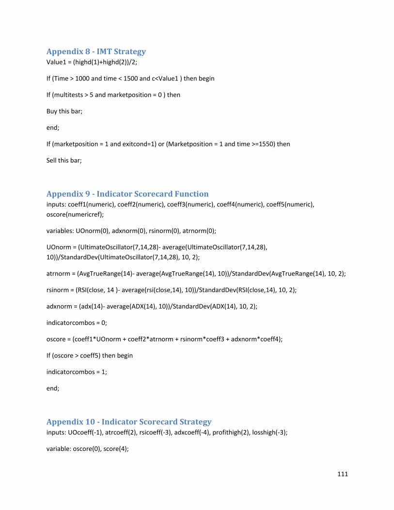
111
Appendix 8 - IMT Strategy Value1 = (highd(1)+highd(2))/2;
If (Time > 1000 and time < 1500 and c<Value1 ) then begin
If (multitests > 5 and marketposition = 0 ) then
Buy this bar;
end;
If (marketposition = 1 and exitcond=1) or (Marketposition = 1 and time >=1550) then
Sell this bar;
Appendix 9 - Indicator Scorecard Function inputs: coeff1(numeric), coeff2(numeric), coeff3(numeric), coeff4(numeric), coeff5(numeric),
oscore(numericref);
variables: UOnorm(0), adxnorm(0), rsinorm(0), atrnorm(0);
UOnorm = (UltimateOscillator(7,14,28)- average(UltimateOscillator(7,14,28),
10))/StandardDev(UltimateOscillator(7,14,28), 10, 2);
atrnorm = (AvgTrueRange(14)- average(AvgTrueRange(14), 10))/StandardDev(AvgTrueRange(14), 10, 2);
rsinorm = (RSI(close, 14 )- average(rsi(close,14), 10))/StandardDev(RSI(close,14), 10, 2);
adxnorm = (adx(14)- average(ADX(14), 10))/StandardDev(ADX(14), 10, 2);
indicatorcombos = 0;
oscore = (coeff1*UOnorm + coeff2*atrnorm + rsinorm*coeff3 + adxnorm*coeff4);
If (oscore > coeff5) then begin
indicatorcombos = 1;
end;
Appendix 10 - Indicator Scorecard Strategy inputs: UOcoeff(-1), atrcoeff(2), rsicoeff(-3), adxcoeff(-4), profithigh(2), losshigh(-3);
variable: oscore(0), score(4);

112
value4 = indicatorcombos(UOcoeff, atrcoeff, rsicoeff, adxcoeff, score, oscore);
If ((Value4 = 1) or (Close< BollingerBand(C, 20, -2))) then begin
Buy this bar;
end;
If (Barssinceentry < 50) then begin
Value2 = C[barssinceentry];
Value3 = 100*((c-value2)/Value2);
end;
If (((((Value3>profithigh) or(Value3<losshigh)) and value4 <1 ) or C>BollingerBand(C,20,2)) and
C>Bollingerband(c,20, -2)) then begin
Sell this bar;
end;
Appendix 11 - Slope Calculating Function inputs: interval1(numeric), interval2(numeric), interval3(numeric), chartinterval(numeric);
variables: interval1u(0), interval2u(0), interval3u(0), slope11(0), slope21(0), slope31(0), hightest(0),
lowtest(0), currenthighest(0), currentlowest(0), secondderiv1(0), secondderiv2(0), secondderiv3(0);
arrays: slope1[5](0), slope2[5](0), slope3[5](0);
interval1u = interval1/chartinterval;
interval2u = interval2/chartinterval;
interval3u = interval3/chartinterval;
For Value1 = 1 to 5 begin
slope1[value1] = ((C of interval1u*(value1-1) bars ago) - (C of interval1u*value1 bars ago))/interval1;
slope2[value1] = ((C of interval2u*(value1-1) bars ago) - (C of interval2u*value1 bars ago))/interval2;
slope3[value1] = ((C of interval3u*(value1-1) bars ago) - (C of interval3u*value1 bars ago))/interval3;
end;
secondderiv1 = (slope1[1] - slope1[2])/interval1;
secondderiv2 = (slope2[1] - slope2[2])/interval2;
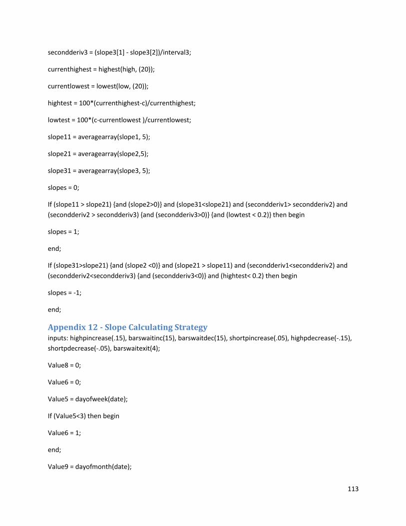
113
secondderiv3 = (slope3[1] - slope3[2])/interval3;
currenthighest = highest(high, (20));
currentlowest = lowest(low, (20));
hightest = 100*(currenthighest-c)/currenthighest;
lowtest = 100*(c-currentlowest )/currentlowest;
slope11 = averagearray(slope1, 5);
slope21 = averagearray(slope2,5);
slope31 = averagearray(slope3, 5);
slopes = 0;
If (slope11 > slope21) {and (slope2>0)} and (slope31<slope21) and (secondderiv1> secondderiv2) and
(secondderiv2 > secondderiv3) {and (secondderiv3>0)} {and (lowtest < 0.2)} then begin
slopes = 1;
end;
If (slope31>slope21) {and (slope2 <0)} and (slope21 > slope11) and (secondderiv1<secondderiv2) and
(secondderiv2<secondderiv3) {and (secondderiv3<0)} and (hightest< 0.2) then begin
slopes = -1;
end;
Appendix 12 - Slope Calculating Strategy inputs: highpincrease(.15), barswaitinc(15), barswaitdec(15), shortpincrease(.05), highpdecrease(-.15),
shortpdecrease(-.05), barswaitexit(4);
Value8 = 0;
Value6 = 0;
Value5 = dayofweek(date);
If (Value5<3) then begin
Value6 = 1;
end;
Value9 = dayofmonth(date);

114
If (value9<7) then begin
Value8 = 1;
end;
If ( ((highw(Value6 +1) - highw(value6))< 0) and ((highm(Value8 +1) - highm(value8))<0) ) then begin
Value7 = time;
If (Value7 < 1550) then begin
Value1 = slopes(1, 5, 10, 1);
if (Value1 = 1) then begin
Buy this bar;
end;
end;
If (Barssinceentry < 50) then begin
Value2 = C[barssinceentry];
Value3 = 100*((c-value2)/Value2);
end;
If (barssinceentry>barswaitexit) then begin
If (value1<1 and (Value3>highpincrease) or ((Barssinceentry>barswaitinc) and (Value3 > shortpincrease))
or (Value3<highpdecrease) or ((barssinceentry>barswaitdec) and (Value3 < shortpdecrease)) or
(slowk(14) crosses above slowd(14))) then begin
Sell this bar;
end;
end;
end;
If Time =1559 then begin
Value12 = 100*(Close - opend(0))/close;
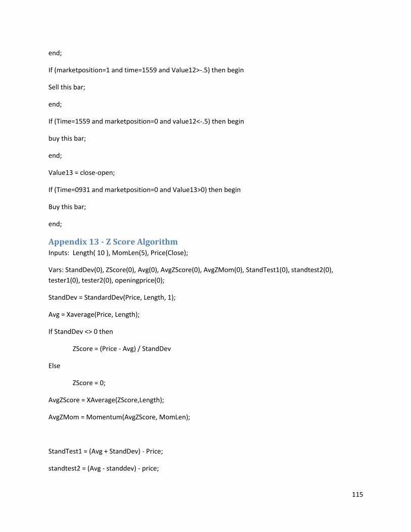
115
end;
If (marketposition=1 and time=1559 and Value12>-.5) then begin
Sell this bar;
end;
If (Time=1559 and marketposition=0 and value12<-.5) then begin
buy this bar;
end;
Value13 = close-open;
If (Time=0931 and marketposition=0 and Value13>0) then begin
Buy this bar;
end;
Appendix 13 - Z Score Algorithm Inputs: Length( 10 ), MomLen(5), Price(Close);
Vars: StandDev(0), ZScore(0), Avg(0), AvgZScore(0), AvgZMom(0), StandTest1(0), standtest2(0),
tester1(0), tester2(0), openingprice(0);
StandDev = StandardDev(Price, Length, 1);
Avg = Xaverage(Price, Length);
If StandDev <> 0 then
ZScore = (Price - Avg) / StandDev
Else
ZScore = 0;
AvgZScore = XAverage(ZScore,Length);
AvgZMom = Momentum(AvgZScore, MomLen);
StandTest1 = (Avg + StandDev) - Price;
standtest2 = (Avg - standdev) - price;
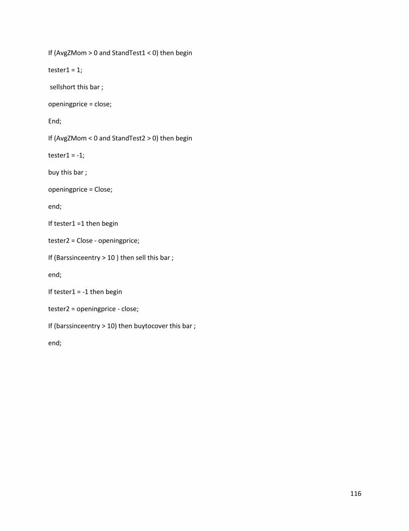
116
If (AvgZMom > 0 and StandTest1 < 0) then begin
tester1 = 1;
sellshort this bar ;
openingprice = close;
End;
If (AvgZMom < 0 and StandTest2 > 0) then begin
tester1 = -1;
buy this bar ;
openingprice = Close;
end;
If tester1 =1 then begin
tester2 = Close - openingprice;
If (Barssinceentry > 10 ) then sell this bar ;
end;
If tester1 = -1 then begin
tester2 = openingprice - close;
If (barssinceentry > 10) then buytocover this bar ;
end;