Embed Size (px)
Citation preview

© 2
013 T
he M
ath
Work
s, In
c.
Developing Customized Measurements and
Automated Analysis Routines using MATLAB®
Guillaume Millot
MathWorks France

2
MathWorks Overview
Founded in 1984 in the US
Several software platforms : MATLAB
Headquarters in Boston
Offices throughout Europe including France, Germany, and the United Kingdom
Used by more than 1,000,000 users in over 175 countries
Used in over 3,500 universities

3
Technical computing language
Development environment
More than 1500 functions Math
2D, 3D graphics and GUI design
File I/O
Calling C/C++, Fortran, Java, COM
Toolboxes for signal and image
processing, connection to hardware
or databases, statistics, optimization, …
Available from MathWorks or Agilent with
Infiniium and InfiniiVision oscilloscopes
and other instruments
MATLAB The leading environment for technical computing

4
Technical Computing Workflow
Reporting and
Documentation
Outputs for Design
Deployment
Share
Explore & Discover
Data Analysis
& Modeling
Files
Software
Hardware
Access
Code & Applications
Automate
Algorithm
Development
Application
Development

5
Measurement, analysis, and testing challenges
for high speed serial and other systems
1. Creating analysis and measurement routines for
designing and testing your system
2. Interfacing and verifying these routines with live
measured data
3. Visualizing analysis routines to improve signal
integrity

6
Measurement, analysis, and testing challenges
for high speed serial and other systems
1. Creating analysis and measurement routines
for designing and testing your system
2. Interfacing and verifying these routines with live
measured data
3. Visualizing analysis routines to improve signal
integrity

7 7
Example: Developing an analysis routine to
perform device characterization
CRj
jT
1
1
In
Out
Goals: 1. Characterize the unknown device (it will be a low-pass filter)
2. Analyze the device (in this case the low-pass filter) to determine if
it behaves as designed
CRFo
2
1
Transfer Function:
Cutoff Frequency:
0 2000 4000 6000 8000 10000 12000-1
0
1
0 2000 4000 6000 8000 10000 12000-1
0
1
0 2000 4000 6000 8000 10000 12000-1
0
1
0 2000 4000 6000 8000 10000 12000-1
0
1 ? V+
V-
V+
V-
R
C In Out

8
Agilent
Signal Generator
8
CR
CRjjT
o
1
1
1
V+
V-
V+
V-
R = 1kW
C = .1mF
Syste
m I
nput
Response
GPIB, LAN, or USB
Agilent
Oscilloscope
Device Characterization Interactively develop your transfer function and analysis
routines
MATLAB

9
Device Characterization Ideal end result
Circuit to be
characterized
Automated Circuit Tool application
developed in MATLAB to characterize
the circuit and determine if it behaves
as designed

10
Demo Clip
11
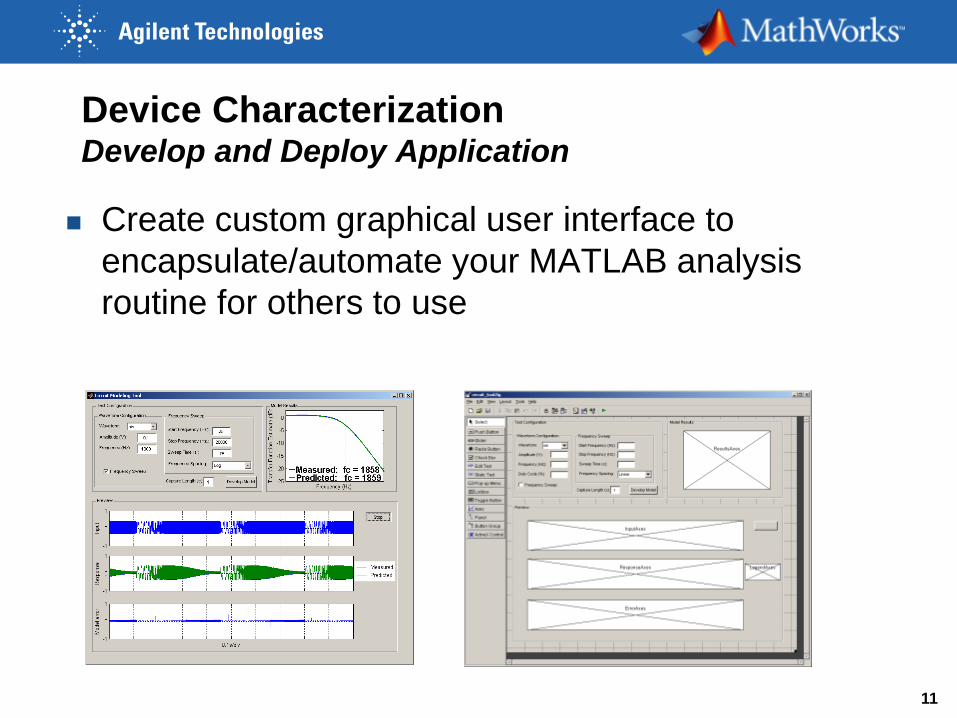
Device Characterization Develop and Deploy Application
Create custom graphical user interface to
encapsulate/automate your MATLAB analysis
routine for others to use

12
Measurement, analysis, and testing challenges
for high speed serial and other systems
1. Creating analysis and measurement routines for
designing and testing your system
2. Interfacing and verifying these routines with
live measured data
3. Visualizing analysis routines to improve
signal integrity

13
MATLAB Connects to Your Hardware Devices
Data Acquisition Toolbox
Plug-in data acquisition devices
and sound cards
Instrument Control Toolbox
Instruments and RS-232
serial devices
MATLAB
Interfaces for communicating
with everything
Image Acquisition Toolbox
Image capture devices
Vehicle Network Toolbox
CAN bus devices using CAN
and XCP protocols

14
Creating a pre-distortion filter and verifying
it with live Agilent oscilloscope signals
Task
– Improve system BER
Solution
– Characterize system’s
response
– Use the characterization
to develop pre-distortion
filter

15
Step 1:
Waveform acquisition from Agilent Oscilloscope
Use Test & Measurement Tool on or off the scope
Test & Measurement Tool provided with MATLAB’s Instrument Control Toolbox

16
Step 2:
Use acquired signals to design pre-distortion filter
Use system identification functions to design FIR pre-distortion filter
-8 -7.95 -7.9 -7.85 -7.8 -7.75 -7.7 -7.65 -7.6 -7.55 -7.5
x 10-7
-0.25
-0.2
-0.15
-0.1
-0.05
0
0.05
0.1
0.15
0.2
0.25
Time
Voltage
With thumb
-8 -7.95 -7.9 -7.85 -7.8 -7.75 -7.7 -7.65 -7.6 -7.55 -7.5
x 10-7
-0.25
-0.2
-0.15
-0.1
-0.05
0
0.05
0.1
0.15
0.2
0.25
Time
Voltage
Sans thumb
In-phase Signal
Time (s)A
mplit
ude (
AU
)0 1 2 3 4 5 6 7
x 10-10
-1
-0.5
0
0.5
1
In-phase Signal
Time (s)
Am
plit
ude (
AU
)
0 1 2 3 4 5 6 7
x 10-10
-1
-0.5
0
0.5
1

17
Step 3: Execute your analysis routines directly on
an Agilent oscilloscope
• Agilent and MathWorks teamed up to create a
custom development environment using
Infiniium oscilloscopes and MATLAB to
address unique and special measurement
needs.
• Requires no knowledge of MATLAB
to operate on the scope
• Agilent automatically includes the MATLAB
software environment as part of the N8806A
UDF option.
17

18
Measurement, analysis, and testing challenges
for high speed serial and other systems
1. Creating analysis and measurement routines for
designing and testing your system
2. Interfacing and verifying these routines with live
measured data
3. Visualizing analysis routines to improve
signal integrity

19
Visualizing MATLAB analysis routines
to improve signal integrity
19
High-speed digital signals are
susceptible to signal integrity issues due
to limitations of the physical interface.
You need: 1. Analysis routines to analyse backplane
behaviour.
2. Acquire live signals from Agilent
instruments to create and verify these
analysis routines.
3. Applications to automate the execution of
these measurement and analysis
routines.
MATLAB provides the capabilities to create analysis routines, interface
to Agilent instruments to acquire live signals to verify them, and
language and tools to automate the execution.

20
MATLAB Code for Acquiring Live Signals from
Agilent instruments
%% Directly acquire digital signals from Agilent oscilloscope or
S-Parameters from Agilent network analyzer ... %% Convert the 16-Port to 4-Port S-Parameters SingleEnded4PortSParams = … snp2smp(SingleEnded16PortData.S_Parameters, … SingleEnded16PortData.Z0, [3 14 4 13]); %% Convert 4-Port to 2-Port Differential S-Parameters Differential2PortSparamsForChannel = … s2sdd(SingleEnded4PortSParams); %% Calculate the Frequency Response DifferentialFreqResponseForChannel = … s2tf(Differential2PortSparamsForChannel); %% Fit Differential Frequency Response to Rational Function ModelforForwardChannel = … rationalfit(Freq, DifferentialFreqResponseForChannel); ...

21
MATLAB Code for Visualizing Jitter of
Acquired Signals
%% First Input and its Output due to CrossTalk InputSignal_1 = GenerateInputsignal(TotalSampleNumber, …); OutputSignal_1 = timeresp(ModelforCrosstalk_1, InputSignal_1, …); %% Second Input and its Output (forward channel) InputSignal_2 = GenerateInputsignal(TotalSampleNumber, …); OutputSignal_2 = timeresp(ModelforForwardChannel,InputSignal_2, …); ... %% The Output Signal of the Second Channel OutputSignal = OutputSignal_1 + OutputSignal_2 + OutputSignal_3 … + OutputSignal_4; %% Eye Diagram of the Output Signal EyeDiagram = commscope.eyediagram('SamplingFrequency', … 1./SampleTime, 'SamplesPerSymbol', OverSamplingFactor) update(EyeDiagram, OutputSignal); %% Jitter Measurements analyze(EyeDiagram); Measurements = EyeDiagram.Measurements

22
Visualizing of Eye Diagram Characteristics
in MATLAB
Total jitter: deterministic jitter and random jitter

23
Visualizing of Eye Diagram Characteristics
in MATLAB (continued)
Deterministic jitter only, no random jitter

24
Measurement, Analysis, and Testing Challenges
Creating analysis and measurement routines for designing and testing your system
MATLAB is a software environment and a programming language made for design and test engineers to be productive
Supports analysis routine creation, data visualization, and application development
Interfacing and verifying these routines with live measured data Integrated measurement and analysis provided with MATLAB
Ability to execute your MATLAB analysis routines directly on Agilent oscilloscopes using N8806A UDF
Visualizing analysis routines to improve signal integrity Analysis routines created in MATLAB can be utilized to visualize
and understand eye diagram characteristics to help improve signal integrity of your high-speed systems

25
Agilent and MATLAB Resources for Developing
Customized Measurement and Analysis Routines
MATLAB overview: www.mathworks.com/matlab
Instrument Control Toolbox overview:
www.mathworks.com/products/instrument
Signal Processing Toolbox overview: www.mathworks.com/products/signal
Agilent resource page on MATLAB for Agilent Infiniium and InfiniiVision
scopes: www.agilent.com/find/matlab_oscilloscopes
Agilent resource page on MATLAB with Agilent instruments:
www.agilent.com/find/matlab
Agilent N8806A User Defined Function: www.agilent.com/find/udf
Using MATLAB to control Agilent oscilloscopes, function generators, and
other instruments www.mathworks.com/agilent

26
EXTRA SLIDES

27
Device Characterization Step 1: Stimulate device and acquire device responses
Configure Agilent signal generator and Agilent
oscilloscope with Instrument Control Toolbox

28
Device Characterization Step 2: Visualize Data
Plot data Select data to plot in the Workspace Browser
Select desired plot type from the Plot button
The equivalent command is displayed in the Command
Window

29
Device Characterization Step 3: Pre-process Data
Scale the data Interactively zoom to explore data – identify scaling problem
Correct scaling with simple MATLAB command

30
Device Characterization Step 4: Visualize Original and Processed Data
Build custom visualization with Plot Tools Enable Plot Tools (plottools) with button on Figure
Toolbar
Drag and drop to layout axes and add data to plots
Customize and annotate plots
Automatically generate MATLAB code to reproduce
visualization with new data

31
Device Characterization Step 5: Estimate Transfer Function
Estimate Transfer Function with the Signal
Processing Toolbox Search the Help for desired functionality
Run sample code directly from the Help Browser
Modify commands for our data

32
Device Characterization Step 6: Compare with Expected Results
Compute expected response with governing equations
Fit theoretical response to measured response with the
Curve Fitting Toolbox Use Curve Fitting Tool to interactively design and analyze a fit to
our data
Automatically generate MATLAB code to compute fit with new data

33
Device Characterization Step 7: Automate Repetition of Analysis
Write custom script to automate workflow Create MATLAB file from selected commands in Command
History
Add comments to generated code in Editor
Use %% to divide code into individual cells to improve
readability and support cell execution

34
Device Characterization Step 8: Publish Results
Publish MATLAB file directly to HTML document Click “Publish to HTML” button in Editor Toolbar
Each cell is converted to a section of the document
All code, comments, and output are captured in the document
35
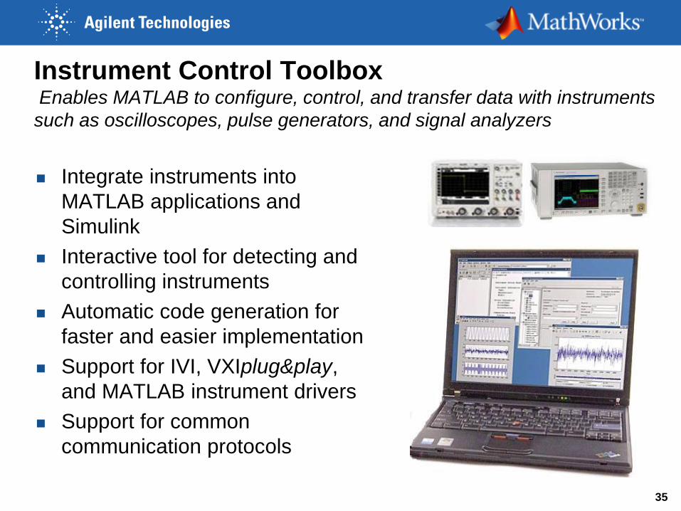
Instrument Control Toolbox Enables MATLAB to configure, control, and transfer data with instruments
such as oscilloscopes, pulse generators, and signal analyzers
Integrate instruments into
MATLAB applications and
Simulink
Interactive tool for detecting and
controlling instruments
Automatic code generation for
faster and easier implementation
Support for IVI, VXIplug&play,
and MATLAB instrument drivers
Support for common
communication protocols

36
Instrument Control Toolbox and
N8806A User Defined Function
Instrument Control Toolbox
Use MATLAB to control the oscilloscope, either on or off the scope, to automate measurements
Download data directly into MATLAB for analysis and to build complete GUI-based test applications.
User Defined Function
Use MATLAB directly on Infiniium oscilloscopes to make customized measurements.

37
N8806A User Defined Function
How to Access
In “Analyze” pull down
menu, click “Math…”
Then select your new
function from the “Operator”
pull down list
37


![MATLAB Mathematical Analysis [2014]](https://img.dokumen.tips/doc/110x75/56d6c06e1a28ab30169a5bff/matlab-mathematical-analysis-2014.jpg)