_____________

Anita Orlowska, Institute of Fundamental Technological Research, Polish Academy of Sciences, Świętokrzyska 21, Warsaw, 00-049, Poland. Jan Holnicki-Szulc, Institute of Fundamental Technological Research, Polish Academy of Sciences, Świętokrzyska 21, Warsaw, 00-049, Poland. Przemyslaw Kolakowski, Institute of Fundamental Technological Research, Polish Academy of Sciences, Świętokrzyska 21, Warsaw, 00-049, Poland.

Title: Monitoring of delamination defects in composite beams

Authors: Anita Orlowska

Jan Holnicki-Szulc

Przemyslaw Kolakowski

ABSTRACT

Damage detection systems based on array of piezoelectric transducers sending

and receiving strain waves have been the subject of intensive research in the last

decade. The signal processing problem is the major challenge in this concept and soft

computing methods are the most often suggested tools for developing a numerically

efficient solver.

Delamination in composite beams is an example of structural defect

considered in this paper. The objective is to propose a new approach to solve the

inverse dynamic problem of structural health monitoring. The first proposition

provides an a posteriori analysis. It is based on the Virtual Distortion Method (VDM),

using the concept of the dynamic influence matrix. The VDM method allows for

decomposition of the dynamic structural response into components caused by external

excitation in an undamaged structure (the linear part) and components describing

perturbations caused by the internal defects in the structure (the nonlinear part). As a

consequence, analytical formulae for calculation of these perturbations and the

corresponding gradients can be derived. Assuming the inspection zone of all possible

defects, a gradient-based optimization algorithm is applied to solve the problem of

defect identification. A numerical tool for delamination identification in double-

layered beams has been developed. An experimental verification of the concept has

been carried out.

The a posteriori VDM-based approach detects and identifies already existing

delaminations. However, sensor system mounted permanently on the operating

structure can also be used for real-time health monitoring. Therefore the second

proposition presented in the paper is the real-time detection system based on

monitoring the strain evolution (measured by piezo-patches) due to the delamination

defect. The advantages and shortcomings of both (a posteriori and real-time)

approaches as well as the possibilities of their application are discussed. Numerical

examples and experimental results are presented.

INTRODUCTION

Delamination is one of the most dangerous kinds of damage. Fast

development of layered materials and composites in last years, is an incentive to look

for effective identification methods. Some techniques based on signal processing have

been proposed, recently. From the mathematical point of view, determination of

damage location and size on the basis of structural response is an optimisation task.

One of the most often suggested approach to develop numerically efficient solver for

this task is soft computing e.g. neural networks, genetic alghoritms.

The crucial point for the identification tools is to have correct numerical model

of delamination. In this paper a proposition of such model will be presented in the

framework of the Virtual Distortion Method (VDM).

VDM FORMULATION

The Virtual Distortion Method allows for fast, efficient reanalysis due to

stiffness modification in structural elements. It means that using information from a

FEM model of the original structure, we are able to obtain structural response after

modification very quickly as a solution of local problem. The most important

definitions for VDM are:

- virtual distortion – a strain generated in an element modeling stiffness modification

in the element (its influence on the structure can be considered as a result similar to

the effect non-homogenous heating)

- influence matrix – collection of structural responses to unit virtual distortion

imposed in every element of the structure successively.

Computation of the influence matrix, which can be realized by introducing

compensative forces equivalent to unit virtual distortions, is the basis for VDM

analysis. The current strain in an element is a superposition of the linear response

(corresponding to undamaged structure) due to external load and the residual response

(corresponding to damaged structure) due to parameter modification:

∑+=+=j

jij

L

i

R

i

L

ii D0εεεεε (1)

The residual response is a linear combination of influence matrix components and

virtual distortions as shown in (1).

The constitutive relation for the structure with introduced virtual distortions yields:

( )0

iiiii AEP εε −= (2)

The internal forces Pi can be also expressed in terms of the modified structure

parameters in the following way:

**

iii AEP = (3)

where Ei, Ai – unmodified parameters, Ei*, Ai

* - parameters after modification. By

comparing (2) and (3), we obtain the formula for a modification coefficient:

i

ii

ii

ii

iAE

AE

ε

εεµ

0** −== (4)

Using this coefficient, equation (1) can be expressed as:

( )∑−+=+=j

jiji

L

i

R

i

L

ii D εµεεεε 1 (5)

Equation (5) can be converted into simple matrix equation bA =0ε , where

the virtual distortion vector is the only unknown.

Introducing the time dimension in VDM approach leads to the Impulse Virtual

Distortion Method (IVDM) formulation, which allows to model dynamic response for

modified structure. The fundamental equation (1) can be written as:

( ) ( ) ( ) ( ) ( ) ( ) ( )∑∑=

−−+=+=τ

τετµεεεε0

1t j

jiji

L

i

R

i

L

ii tDtttt (6)

Influence matrix elements in this case are computed as structural elements responses

to a time-dependent unit virtual distortion.

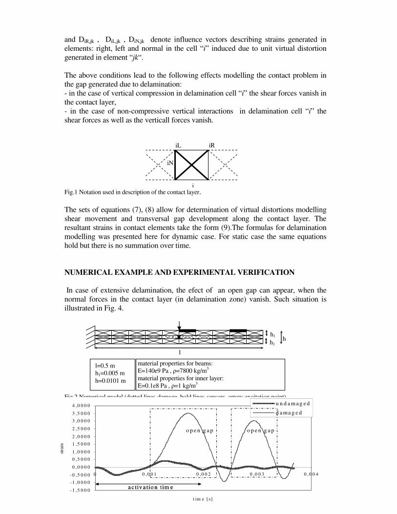
DELAMINATION MODELLING ALGHORITM

The VDM/IVDM have been applied for modeling of delamination in a double

layered beam. The idea was to build a numerical model of a structure (Fig. 2) with a

special, very thin layer between two beams. This extra layer, called in the paper

contact layer, can be interpreted as a glue layer in a real structure.

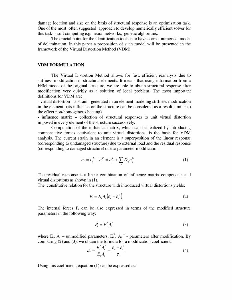
In the modelling of contact layer the following conditions have been imposed on the

pair of inclined elements (left and right) and on the vertical one in each delamination

modelling cell “i” (cf. Fig.1):

- in the case of vertical compression in delamination cell “i”:

( ) ( ) ( ) ( )tttt iLiLiRiR εεεε == 00

(7)

( ) ( )tt iNiN εε =0

- in the case of non-compressive vertical interactions in delamination cell “i”:

( ) ( ) ( ) ( )tttt iLiLiRiR εεεε == 00

(8)

( ) 00 =tiNε

where:

( ) ( ) ( ) ( )τετεετ

∑∑=

−+=0 ,

0

,

t kj

jkjkiR

L

iRiR tDtt ; ( ) ( ) ( ) ( )∑∑=

−+=τ

τετεε0 ,

0

,

t kj

jkjkiL

L

iLiL tDtt

(9)

( ) ( ) ( ) ( )τετεετ

∑∑=

−+=0 ,

0

,

t kj

jkjkiN

L

iNiN tDtt ; NLRk ,,=

and DiR,jk , DiL,jk , DiN,jk denote influence vectors describing strains generated in

elements: right, left and normal in the cell “i” induced due to unit virtual distortion

generated in element “jk“.

The above conditions lead to the following effects modelling the contact problem in

the gap generated due to delamination:

- in the case of vertical compression in delamination cell “i” the shear forces vanish in

the contact layer,

- in the case of non-compressive vertical interactions in delamination cell “i” the

shear forces as well as the verticall forces vanish.

Fig.1 Notation used in description of the contact layer.

The sets of equations (7), (8) allow for determination of virtual distortions modelling

shear movement and transversal gap development along the contact layer. The

resultant strains in contact elements take the form (9).The formulas for delamination

modelling was presented here for dynamic case. For static case the same equations

hold but there is no summation over time.

NUMERICAL EXAMPLE AND EXPERIMENTAL VERIFICATION

In case of extensive delamination, the efect of an open gap can appear, when the

normal forces in the contact layer (in delamination zone) vanish. Such situation is

illustrated in Fig. 4.

Fig.2 Numerical model (dotted lines-damage, bold lines-sensors, arrow-excitation point).

- 1 ,5 0 0 0

- 1 ,0 0 0 0

- 0 ,5 0 0 0

0 ,0 0 0 0

0 ,5 0 0 0

1 ,0 0 0 0

1 ,5 0 0 0

2 ,0 0 0 0

2 ,5 0 0 0

3 ,0 0 0 0

3 ,5 0 0 0

4 ,0 0 0 0

0 0 ,0 0 1 0 ,0 0 2 0 ,0 0 3 0 ,0 0 4

t im e [ s]

stra

in

u n d a m a g e d

d a ma g e d

a c tiv a tio n tim e

o p e n g a po p e n g a p

- 1 ,5 0 0 0

- 1 ,0 0 0 0

- 0 ,5 0 0 0

0 ,0 0 0 0

0 ,5 0 0 0

1 ,0 0 0 0

1 ,5 0 0 0

2 ,0 0 0 0

2 ,5 0 0 0

3 ,0 0 0 0

3 ,5 0 0 0

4 ,0 0 0 0

0 0 ,0 0 1 0 ,0 0 2 0 ,0 0 3 0 ,0 0 4

t im e [ s]

stra

in

u n d a m a g e d

d a ma g e d

a c tiv a tio n tim ea c tiv a tio n tim e

o p e n g a po p e n g a p

l

h1

h1 h

l=0.5 m

h1=0.005 m

h=0.0101 m

material properties for beams:

E=140e9 Pa , ρ=7800 kg/m3

material properties for inner layer:

E=0.1e8 Pa , ρ=1 kg/m3

iL iR

i

iN

Fig.3 Extensive delamination case - responses of the undamaged and damaged structure for vertical

element localized inside the delaminated zone.

The damage was localized in the middle part of the structure (elements marked as

dotted lines) and delamination crack size was near 1/3 length of the beam.

As it is shown in Fig. 4c, when the strains for a vertical element placed in the

damaged region (bold line) become positive, virtual distortions 0

iβ take non-zero

values (it’s the open gap situation).

The experimental verification of the delamination modeling alghoritm was

done for a simple structure built from two beams connected in ten points by screws.

The structure was excited by a windowed signal, which was applied to the

piezoelectric actuator mounted near the clamped end. Structural response was

collected using piezoelectric patch glued near the free end. The results are presented in

Fig. 4.

Fig.4 Experimental verification results: real structure with vertical lines as screws and numerical model

with contact layer (dotted lines correspond damaged screws) (a), experimental and numerical response

comparison (b).

VDM APPROACH IN DELAMINATION MONITORING

We shall pose the optimisation problem of structural damage identification

(constraining ourselves temporarily to the static case) within the framework of the

Virtual Distortion Method (cf. [4]). Let us minimise the following function:

( )∑ ε−εA

2

A

M

Amin (10)

sensor

sensor actuator

actuator

a)

b)

-0,06

-0,04

-0,02

0

0,02

0,04

0,06

0 500 1000 1500

time [au.]

stra

in [

au.]

damaged - experimental responseundamageddamaged - numerical response

which can be interpreted as an average departure of the total structural strain

εA from the in-situ measured strain εAM

in damaged locations A. Taking advantage of

the VDM formulation we can decompose the strain εA into two parts:

∑ ε+ε=ε+ε=εA

o

iAi

L

A

R

A

L

AA D (11)

As the component εAL is constant for a given external load, the so-called

residual strain component εAR may only be varying in the optimisation process with

the virtual distortion εo as the design variable.

We shall measure the structural damage in each member i with the help of the

coefficient µi i.e. with the ratio of cross-sectional areas of a damaged member to the

undamaged one. Consequently we have to impose appropriate constraints on this

coefficient. As we examine the physical process of deterioration of the member cross-

section we are interested in such µi, which complies with the following constraints:

10.e.i10i

o

iii ≤

ε

ε−ε≤≤µ≤

(12)

For delamination problems the coefficient µ will finally (after optimisation) take only

two values: 0 (delamination) or 1 (full connection).

The gradients of the objective function and the constraints are expressed in

terms of the design variable εo as follows:

( )∑ ε−ε−=ε∂

∂=∇

AA

M

AAko

k

D2f

f

(13)

and

( )2

l

o

llkllk

o

k

lkl

DgnN

ε

ε−εδ=

ε∂

∂==

(14)

In order to solve the damage identification problem posed by (10) and (12) the

Gradient Projection Method (cf. [1], [2], [3]) can be used as optimisation tool. The

Gradient Projection Method is based on the idea of projecting the search direction (i.e.

the direction in which the objective function value decreases) into the subspace

tangent to the active constraints.

NUMERICAL TESTS

Let’s discuss the case of damage located in section 5 (Fig. 5). The excitation signal is

one period of the sinusoidal wave of the frequency corresponding to 4th natural

frequency of the undamaged structure (666.16 Hz). The initial gradient values are

very important for the optimization routine. For the one-section delamination damage

case, the gradient disturbance has a localized character. It means that optimal sensor

location is near the damaged section (initial gradients for sensors placed long distance

from damage are flat).

There will be two cases of sensor location compared. In the case of one sensor

placed near the free end of the structure, gradient values at the begining of the

optimization process are at the same level (do not show that damage is localized in

section 5). After 80 iterations the goal function value is approaching zero but still

decreasing. As shown in Fig. 6a the damage coefficient for section 5 is also near zero.

It seems to be promising for identification but very time-consuming.

In the case of three sensors the first gradient with index 5 is at higher level

than others, and we have quite good identification results already after 20 iterations

(Fig. 6b).

The computation of gradients for this case was done for every of the three sensors (in

every optimization iteration). The way for doing computation faster is to evaluate the

most possible location of damage (using results from a few sensors) and compute

gradients only for the sensor with the biggest difference between the damaged and

undamaged response.

Fig.5 Truss-structure model (not scaled) with the sensors (bold lines) and the excitation point (arrow) .

Fig. 6 Identification results for one sensor (a) and for three sensors (b).

REAL-TIME DETECTION OF DELAMINATION

The previously discussed cases can be considered as a posteriori testing detecting

and identifying already existing delaminations. However, in many applications a real-

time health monitoring is the challenge. Having sensor system mounted permanently

on the operating structure, the damage detection “in motion” seems to be feasible. Let

us discuss the case of our testing beam under steady-state excitation with delemination

(in section No.5) generated during exploitation.

l=0.5 m

h1=0.005 m

h=0.0101 m

material properties for beams:

E=140e9 Pa , ρ=7800 kg/m3

material properties for inner layer:

E=140e9 Pa , ρ=1 kg/m3

l

h1

h1 h

0,00

0,50

1,00

1,50

1 2 3 4 5 6 7 8 9 10

section number

damage coefficient

0,00

0,50

1,00

1,50

1 2 3 4 5 6 7 8 9 10 section number

damage coefficient

a)

b)

Fig.7 Field between damaged and undamaged response for delamination in section 5.

Fig.8 Field between damaged and undamaged response for delamination in sections 5 and 6.

The field between standard response on steady-state excitation and response changed

by delamination computed for each sensor are shown in Fig. 7, 8.

Alghoritm for automatic identification of delamination based on the above results can

be proposed. The algorithm can be based on determination of the pair of two sensors

with maximal average signal. The delamination area is located in-between these

maximally loaded sensors. The example with more extended delamination (in

elements No. 5 and 6) is shown in Fig. 8, where locations of maximally loaded

sensors determine the length of the defect.

Acknowledgement We kindly acknowledge the research programs DIADYN, PBZ-KBN-105/T10/2003, 2005-

2008 and RTN SMART-SYSTEMS, HPRN-CT-2002-00284, 2002-2006

REFERENCES

1. Rosen J. B. (1960) The Gradient Projection Method for Nonlinear Programming, Part I – Linear

Constraints, SIAM Journal of Applied Mathematics, 8(1), pp. 181-217

2. Rosen J. B. (1961) The Gradient Projection Method for Nonlinear Programming, Part II –

Nonlinear Constraints, SIAM Journal of Applied Mathematics, 9(4), pp. 514-532

3. Haug E. J., Arora J. S. (1979) Applied Optimal Design: Mechanical and Structural Systems,

John Wiley & Sons, New York, U.S.A.

4. Holnicki-Szulc,J, T.Zielinski, New damage Identification Method Through the Gradient Based

Optimisation, Proc. COST International Conference on System Identification & Structural

Health Monitoring, Madrid, 6-9 Jun 2000

0,0E+00

4,0E-09

8,0E-09

1,2E-08

1,6E-08

1 2 3 4 5 6 7 8 9 10 section number

fiel

d b

etw

een

dam

aged

and

undam

aged

res

ponse

fiel

d b

etw

een

dam

aged

and

undam

aged

res

ponse

section number

0,0E+00

1,0E-08

2,0E-08

3,0E-08

1 2 3 4 5 6 7 8 9 10