Embed Size (px)
Citation preview

Australian Rainfall & Runoff
Revision Projects
PROJECT 18
Interaction of Coastal Processes And Severe Weather Events
P18/S2/010
JUNE 2012
Engineers Australia Engineering House 11 National Circuit Barton ACT 2600 Tel: (02) 6270 6528 Fax: (02) 6273 2358 Email:[email protected] Web: www.engineersaustralia.org.au
AUSTRALIAN RAINFALL AND RUNOFF REVISION PROJECT 18: INTERACTION OF COASTAL PROCESSES AND SEVERE WEATHER EVENTS
STAGE 2 REPORT
JUNE, 2012
Project Revision Project 18: Interaction of Coastal Processes and Severe Weather Events
AR&R Report Number P18/S2/010
Date 13 June 2012
ISBN 978-085825-8747
Contractor UNSW Water Research Centre
Contractor Reference Number 2011/2
Authors Seth Westra
Verified by
Revision Project
P18/S2/010 : 13 June 2012
This project was made possible by fundin
Department of Climate Change. This report and the associate
significant amount of in kind hours provided by Engineers Australia Members.
Revision Project 18: Interaction of Coastal Processes and Severe Weather Events
ACKNOWLEDGEMENTS
This project was made possible by funding from the Federal Government through the
epartment of Climate Change. This report and the associated project are the result of a
significant amount of in kind hours provided by Engineers Australia Members.
Contractor Details
UNSW Water Research Centre The University of New South Wales
Sydney, NSW, 2052
Tel: (02) 9385 5017 Fax: (02) 9313 8624
Web: http://water.unsw.edu.au
18: Interaction of Coastal Processes and Severe Weather Events
i
Federal Government through the
project are the result of a
significant amount of in kind hours provided by Engineers Australia Members.

Revision Project 18: Interaction of Coastal Processes and Severe Weather Events
P18/S2/010 : 13 June 2012 ii
FOREWORD
AR&R Revision Process
Since its first publication in 1958, Australian Rainfall and Runoff (ARR) has remained one of the
most influential and widely used guidelines published by Engineers Australia (EA). The current
edition, published in 1987, retained the same level of national and international acclaim as its
predecessors.
With nationwide applicability, balancing the varied climates of Australia, the information and the
approaches presented in Australian Rainfall and Runoff are essential for policy decisions and
projects involving:
• infrastructure such as roads, rail, airports, bridges, dams, stormwater and sewer
systems;
• town planning;
• mining;
• developing flood management plans for urban and rural communities;
• flood warnings and flood emergency management;
• operation of regulated river systems; and
• prediction of extreme flood levels.
However, many of the practices recommended in the 1987 edition of AR&R now are becoming
outdated, and no longer represent the accepted views of professionals, both in terms of
technique and approach to water management. This fact, coupled with greater understanding of
climate and climatic influences makes the securing of current and complete rainfall and
streamflow data and expansion of focus from flood events to the full spectrum of flows and
rainfall events, crucial to maintaining an adequate knowledge of the processes that govern
Australian rainfall and streamflow in the broadest sense, allowing better management, policy
and planning decisions to be made.
One of the major responsibilities of the National Committee on Water Engineering of Engineers
Australia is the periodic revision of ARR. A recent and significant development has been that
the revision of ARR has been identified as a priority in the Council of Australian Governments
endorsed National Adaptation Framework for Climate Change.
The update will be completed in three stages. Twenty one revision projects have been identified
and will be undertaken with the aim of filling knowledge gaps. Of these 21 projects, ten projects
commenced in Stage 1 and an additional 9 projects commenced in Stage 2. The remaining two
projects will commence in Stage 3. The outcomes of the projects will assist the ARR Editorial

Revision Project 18: Interaction of Coastal Processes and Severe Weather Events
P18/S2/010 : 13 June 2012 iii
Team with the compiling and writing of chapters in the revised ARR.
Steering and Technical Committees have been established to assist the ARR Editorial Team in
guiding the projects to achieve desired outcomes. Funding for Stages 1 and 2 of the ARR
revision projects has been provided by the Federal Department of Climate Change and Energy
Efficiency. Funding for Stages 2 and 3 of Project 1 (Development of Intensity-Frequency-
Duration information across Australia) has been provided by the Bureau of Meteorology.
Project 18: Interaction of coastal processes and severe weather events
Flooding in the downstream regions of many coastal catchments is the result of the interaction
between runoff generated by a weather event that elevates sea levels and/or estuary water
levels. Historically assumptions have been made regarding either the independence of these
events or the timing of rainfall or flood peaks and peak ocean and/or estuarine conditions, for
example peak runoff and peak ocean or estuary levels coinciding. Assuming that the weather
events that generated elevated ocean or estuary conditions and significant catchment runoff are
independent can underestimate flood levels in coastal areas. Conversely an assumption that
the flood peak coincides with the peak elevated ocean or estuary conditions can overestimate
flood levels in coastal areas. In order to better understand flooding in coastal areas it is
necessary to have an understanding of the role that severe weather conditions that create
elevated ocean or estuary conditions have in generating catchment runoff that floods coastal
areas.
The importance of this understanding will increase in time as existing coastal communities are
threatened increasingly by sea level rise as a result of climate change.
Mark Babister Assoc Prof James Ball
Chair Technical Committee for ARR Editor
ARR Research Projects

Revision Project 18: Interaction of Coastal Processes and Severe Weather Events
P18/S2/010 : 13 June 2012 iv
AR&R REVISION PROJECTS
The 21 AR&R revision projects are listed below:
ARR Project No. Project Title Starting Stage
1 Development of intensity-frequency-duration information across Australia 1
2 Spatial patterns of rainfall 2
3 Temporal pattern of rainfall 2
4 Continuous rainfall sequences at a point 1
5 Regional flood methods 1
6 Loss models for catchment simulation 2
7 Baseflow for catchment simulation 1
8 Use of continuous simulation for design flow determination 2
9 Urban drainage system hydraulics 1
10 Appropriate safety criteria for people 1
11 Blockage of hydraulic structures 1
12 Selection of an approach 2
13 Rational Method developments 1
14 Large to extreme floods in urban areas 3
15 Two-dimensional (2D) modelling in urban areas. 1
16 Storm patterns for use in design events 2
17 Channel loss models 2
18 Interaction of coastal processes and severe weather events 1
19 Selection of climate change boundary conditions 3
20 Risk assessment and design life 2
21 IT Delivery and Communication Strategies 2
AR&R Technical Committee:
Chair: Mark Babister, WMAwater
Members: Associate Professor James Ball, Editor AR&R, UTS
Professor George Kuczera, University of Newcastle
Professor Martin Lambert, Chair NCWE, University of Adelaide
Dr Rory Nathan, SKM
Dr Bill Weeks, Department of Transport and Main Roads, Qld
Associate Professor Ashish Sharma, UNSW
Dr Bryson Bates, CSIRO
Steve Finlay, Engineers Australia
Related Appointments:
ARR Project Engineer: Monique Retallick, WMAwater
Assisting TC on Technical Matters: Dr Michael Leonard, University of Adelaide

Revision Project 18: Interaction of Coastal Processes and Severe Weather Events
P18/S2/010 : 13 June 2012 v
PROJECT TEAM
Project team: This project was led by Dr Seth Westra (UNSW Water Research Centre) with
specialist statistical input from Dr Scott Sisson (UNSW Department of Mathematics and
Statistics).
Acknowledgements: Discussions with a number of people assisted in the compilation of this
report. Specifically, I would like to acknowledge Dr John Hunter who provided valuable feedback
on the Australian storm surge record and the meteorological drivers of surge; Mr Kirby
Campbell-Wood for assisting with data compilation and testing; Drs Peter Hawke (HR
Wallingford) and Cecilia Svensson (UK Centre of Ecology and Hydrology) for providing
information on the methodology currently used in the UK; Mr Paul Davill (National Tidal Centre)
for providing input on the storm tide data used in this project; and Mr Mark Babister and Ms Erin
Askew (WMAwater) for providing the hydrodynamic modelling results for the Hawkesbury-
Nepean estuary.
The tidal data was collated by Mr Alex Osti from EngTest at Adelaide University, with further
details on the dataset provided in a separate report (EngTest, 2010). This involved obtaining
licences to use data from a range of harbour and port authorities, which are listed as follows:
• Sydney Ports Corporation;
• Maritime Authority of NSW;
• Newcastle Port Corporation;
• Port Kembla Port Corporation;
• Department of Planning and Infrastructure, Northern Territory;
• Maritime Safety Queensland;
• Flinders Ports;
• TasPorts;
• Victorian Regional Channels Authority;
• Port of Melbourne Corporation;
• Bureau of Meteorology;
• Port of Portland;
• Patrick Ports;
• Albany Port Authority;
• Broome Port Authority;
• Bunbury Port Authority;
• Coastal Data Centre,
• WA Department of Transport;
• Esperance Ports Sea and Land;
Revision Project 18: Interaction of Coastal Processes and Severe Weather Events
P18/S2/010 : 13 June 2012 vi
• Fremantle Ports;
• Geraldton Port Authority;
• Dampier Port Authority; and
• Port Headland Port Authority.
This report was independently reviewed by:
• Associate Professor Andrew Metcalfe, University of Adelaide
• Associate Professor Pieter van Gelder, Delft University of Technology
Revision Project 18: Interaction of Coastal Processes and Severe Weather Events
P18/S2/010 : 13 June 2012 vii
EXECUTIVE SUMMARY
Flooding in the lower reaches of many coastal catchments can result from runoff generated by
an extreme precipitation event occurring over the catchment, and/or elevated tail water levels
attributable to a combination of high astronomical tide and storm surge. In many cases these
flood-producing processes are the result of common meteorological conditions, with elevated
storm surges being more likely to occur on days with extreme inland precipitation than on other
days. This issue, referred to as joint dependence, can result in higher flood levels compared to
the case where these processes are independent. The degree to which these processes tend to
co-occur around the Australian coastline, however, is still not known.
This report presents the outcomes of a pilot study into the application of statistical joint
probability methods on extreme rainfall and storm surge in the coastal zone, with a view to
providing guidance on the degree of interaction between these two physical process, as well as
describing how this information should be applied for the estimation of flood risk along the
Australian coastline. As part of this study, three separate areas of work were conducted: (1) the
compilation of a large dataset of historical storm tide records at a number of locations along the
Australian coastline, which when combined with the existing records of daily and sub-daily
rainfall, can form the basis of an empirical study on the joint dependence between these
variables; (2) a review of the statistical extreme value modelling literature with the objective of
developing a model that can identify the strength of dependence between these variables; and
(3) the identification of a methodology by which information on dependence between extreme
rainfall and storm surge can be translated to a flood variable (such as a flood level or flow rate)
at any location along the Australian coastline. The outcomes of each of these items are
summarised briefly below.
The storm tide data collected for this project was obtained from two sources. The first, obtained
from the Australian Baseline Sea Level Monitoring Project (ABSLMP), comprises 16 tide gauges
along the coastline, with records spanning from 1991 to 2010. This dataset is near complete
(less than 2% missing), and additional information including sea level pressure and wind speed
is also available at each location. The second dataset comprises a set of 74 tide gauges
obtained from a number of different port authorities around Australia, of which there are 12
gauges with more than 45 years of record, and a further 12 gauges with more than 30 years of
record. This dataset does not provide information on other meteorological variables, however,
and in some cases there are significant periods of missing records. Nevertheless, it is the latter
dataset which has been used for further analysis in this report, due to the longer length of some
of the records.
Revision Project 18: Interaction of Coastal Processes and Severe Weather Events
P18/S2/010 : 13 June 2012 viii
After a review of a range of bivariate extreme value models which have been applied to model
extremal dependence, a bivariate point process model described in Coles and Tawn (1994) was
ultimately selected. The advantage of this formulation is that extremes are defined in terms of a
distance from the origin (after transformation of both marginal distributions to a unit-Fréchet
distribution), such that it is possible to account for situations where flooding is caused by only a
single process variable being extreme (i.e., an extreme rainfall event occurring in the absence of
any storm surge, or an extreme ocean level occurring in the absence of any rainfall), or by both
processes being extreme simultaneously. In contrast, the better known bivariate threshold
excess models are only applicable when both variables are above some high threshold, and
therefore do not cover the case where extreme flooding occurs as a result of only a single
process being extreme.
To evaluate the performance of this model and identify the extent to which extreme rainfall and
storm surge are dependent, this model was applied to three locations along the east Australian
coastline: Sydney, Brisbane and Mackay. The outcomes of this analysis were as follows:
(1) Statistically significant dependence between extreme rainfall and storm surge could be
found at each of these locations, with greatest dependence in Brisbane and least
dependence at Mackay. It is possible that the high dependence in Brisbane is partly due
to the location of the tide gauge at the mouth of the Brisbane River, as the storm tide
records may be influenced by catchment flows as well as ocean influences. In contrast,
in the case of Sydney and Mackay it is less likely that the storm tide records are
contaminated by catchment flows, and thus the dependence at these locations is
expected to represent the true dependence between rainfall and storm surge.
(2) When considering the effect of distance between tide gauge and the rain gauge,
dependence could be observed over distances of at least several hundred kilometres at
each of the three tide gauge locations. Similarly, the effect of lag between rainfall event
and storm tide event was also considered, with the greatest level of dependence found
when the events occurred concurrently, although the dependence remained high for lags
of up to several days. These combined results suggest that dependence issues need to
be considered even for large catchments with response times of several days.
(3) The effect of storm burst duration was tested by considering storm bursts from 6 minutes
through to 72 hours. Based on this analysis it was concluded that the dependence
between rainfall and storm tide is heavily influenced by storm burst duration, with
relatively small levels of dependence for short durations (particularly sub-hourly
durations) and dependence increasing gradually for longer durations. This has significant
implications for flood estimation, as floods from small catchments with sub-hourly
Revision Project 18: Interaction of Coastal Processes and Severe Weather Events
P18/S2/010 : 13 June 2012 ix
response times are likely to be less affected by joint dependence issues than would be
the case for larger catchments.
Having identified the strength of dependence between rainfall and storm tide, the final issue is to
convert this information into a flood variable such as the flood level at any desired location.
Using hydrologic and hydrodynamic modelling in the Hawkesbury-Nepean as a case study, an
approach was developed in which the flood levels are estimated at a given location for a range
of combinations of catchment flows and ocean levels (represented in terms of their respective
exceedance probabilities), and these levels superimposed onto the bivariate dependence
model. The flood levels at a range of exceedance probabilities up to the 1% AEP (annual
exceedance probability) were estimated for the situations of complete dependence, complete
independence and two intermediate dependence levels, with these results showing that even
with relatively small dependence between rainfall and storm surge, the implication on flood
levels can be significant.
A methodology is proposed which may be suitable for inclusion in the forthcoming Australian
Rainfall and Runoff flood estimation guidelines. This methodology commences with a pre-
screening step which identifies whether joint probability modelling is in fact necessary, based on
(1) whether the dependence is likely to be significant at the location of interest; and (2) whether
the difference in flood levels between the complete independence and complete dependence
situation is sufficient to warrant more detailed modelling. Having determined that joint probability
modelling is necessary at a particular location, the next step is to estimate the dependence
parameter relevant for that specific location, potentially using the catchment response time as
the basis for identifying the critical storm burst duration. It is proposed that maps be provided
around the Australian coastline with an estimate of the dependence parameter, derived for a
range different storm burst durations, and that these be used as the basis of this information.
Finally, the approach used for the Hawkesbury-Nepean river system to convert dependence into
a flood variable is recommended for more general use, and will involve running a
hydrologic/hydrodynamic model a number of times with different combinations of catchment
flows and ocean levels, in order to estimate the flood variable at the desired exceedance
probability.
Given the pilot nature of this study, a range of outstanding research areas were identified which
should be addressed prior to the development of the guidelines. Of these areas, three are likely
to require most attention: (1) further investigation into the specific form of dependence model,
focusing on the capability of the models to simulate the case where the data are either
independent or nearly independent; (2) application of the selected dependence model to a larger
number of locations throughout Australia, to develop the spatial maps of dependence parameter
around the Australian coastline; and (3) further testing of the approach at different case study

Revision Project 18: Interaction of Coastal Processes and Severe Weather Events
P18/S2/010 : 13 June 2012 x
locations, to provide guidance on implementation of the hydrologic and hydrodynamic modelling
to account for this dependence.

Revision Project 18: Interaction of Coastal Processes and Severe Weather Events
P18/S2/010 : 13 June 2012 xi
Table of Contents
1. Introduction ............................................................................................................... 1
1.1. Background ................................................................................................ 1
1.2. Scope of pilot study and report outline ........................................................ 3
2. Data ............................................................................................................................ 5
2.1. Tidal records ............................................................................................... 5
2.2. Rainfall Records ....................................................................................... 13
2.3. Additional data .......................................................................................... 15
3. Methodology ........................................................................................................... 17
3.1. Brief Overview of Univariate Extreme Value Theory ................................. 18
3.2. Modelling Dependence of Bivariate Extremes ........................................... 21
3.2.1. Component-wise block maxima approach ................................................ 21
3.2.2. Threshold excess approach ...................................................................... 23
3.2.3. Point process approach ............................................................................ 24
3.2.4. Structure variable approach ...................................................................... 25
3.2.5. Additional issues ....................................................................................... 26
4. Applying the joint dependence model to Fort Denison storm surge data .......... 29
5. Modelling dependence at selected locations ........................................................ 38
5.1. Dependence with daily rainfall and influence of distance to tide gauge ..... 39
5.2. Influence of lag between daily rainfall and storm surge ............................. 44
5.3. Influence of storm burst duration ............................................................... 46
6. Case study: Hawkesbury Nepean model .............................................................. 48
6.1. Background .............................................................................................. 48
6.2. Modelling flood height ............................................................................... 49
7. Conclusions and Recommendations .................................................................... 58
7.1. Research summary ................................................................................... 58
7.2. Recommended form of guidance into joint dependence of extreme rainfall
and storm surge in the coastal zone ......................................................... 60
7.3. Recommendations for further research ..................................................... 63

Revision Project 18: Interaction of Coastal Processes and Severe Weather Events
P18/S2/010 : 13 June 2012 xii
8. References .............................................................................................................. 66
Appendix 1 – Information on the rain gauges used in the analysis of Chapter 5. .............. 69
A1.1: Rain gauges near Fort Denison tide gauge ...................................................... 69
A1.2: Rain gauges near Brisbane tide gauge ............................................................ 70
A1.3: Rain gauges near Mackay tide gauge .............................................................. 71
Revision Project 18: Interaction of Coastal Processes and Severe Weather Events
P18/S2/010 : 13 June 2012 1
1. Introduction
1.1. Background
Flooding in the lower reaches of many coastal catchments can result both from the runoff
generated by an extreme precipitation event occurring over the catchment, or from elevated
ocean levels due to a combination of high astronomical tide and storm surge. In many cases
these flood-producing mechanisms are the result of common meteorological forcings, with
elevated storm surges being more likely to occur on days with extreme inland precipitation than
at other times. This can result in higher flood risk along the coastal zone compared to what
would be the case if these processes were independent, highlighting the need for flood
estimation methods which take such interactions into account.
The presence of statistical dependence between the extremes of precipitation and storm surge
is well known, and is due to the common meteorologic conditions that often give rise to both
types of extremes. For example, Pugh (1987) highlights the important role of winds and
atmospheric pressure anomalies in determining the magnitude of storm surge, with similar low
pressure systems often associated with heavy rainfall. Such interactions also have been
described statistically by numerous authors (e.g. Hawkes, 2006; Hawkes and Svensson, 2005;
Loganathan et al., 1987; Svensson and Jones, 2002; Svensson and Jones, 2004), with
Svensson and Jones (2004) showing that the relationship between storm surge and rainfall or
catchment discharge can be complex, governed by a range of factors including location,
catchment orientation and the lag between the extreme rainfall and extreme storm surge event.
In parallel or often preceding these findings has been the significant progress in the
development of statistical techniques for characterising dependence in multivariate extreme
events, which by definition occur at the tail ends of a probability distribution and are therefore
sparsely sampled. Commencing with early theoretical work by de Haan and Resnick (1977) and
Pickands (1981), such multivariate extreme value methods have proved much more difficult to
implement in practice compared to their univariate counterparts, due to the additional
mathematical complexities involved in characterising multivariate extremes, as well as
conceptual difficulties related to defining a multivariate extreme event (e.g. see discussions in
Katz et al., 2002; Yue and Rasmussen, 2002). Nevertheless, the class of bivariate and
multivariate extreme value distributions now provide the common modelling framework used to
simulate a range of extreme multivariate processes, with many of the published applications
related to extreme wave height and storm surge (Bortot et al., 2000; Coles et al., 1999; Coles
and Tawn, 1994), still water level and wave height (Hawkes et al., 2002), wave height and wave
period (Callaghan and Helman, 2008), and extreme storm surge and rainfall or catchment
discharge (Hawkes and Svensson, 2005; Svensson and Jones, 2004).

Revision Project 18: Interaction of Coastal Processes and Severe Weather Events
P18/S2/010 : 13 June 2012 2
Having characterised the strength of dependence between two or more physical processes
which have an influence on flooding at a particular location, the next logical question is: how can
this information be applied to estimate flood quantiles at some desired return interval? This is a
much more challenging problem than the situation where floods are caused by only a single
physical process, because the return period of the forcing processes are no longer equivalent to
the return period of the flood (Callaghan and Helman, 2008; Hawkes et al., 2002). To address
this issue, Coles and Tawn (1994) describe a method for translating the extremes of two or
more constituent processes into the design variable of interest via a boundary function (also
known as a ‘limit state function’ in the context of structural design, or simply as the ‘joint
probability method’ (e.g. Hawkes, 2008), whereas other authors focus on reducing the
multivariate process to the variable of interest followed by application of univariate extreme
value theory to estimate the design event (often referred to as the 'structure variable method';
see Bortot et al., 2000). In providing guidance to flood estimation practitioners, the UK
Department of Environment, Food and Rural Affairs (DEFRA) has outlined two methods for
estimating joint dependence of streamflow and surge, as well as rainfall and surge, in the
coastal zone (Hawkes and Svensson, 2005; Hawkes and Svensson, 2006; Svensson and
Jones, 2006), and then translating this into flood levels. These methods differ by their data
requirements and complexity of implementation; however both approaches are developed for
estimation of flood quantiles when two or more physical processes are expected to play
significant roles, and both are designed for implementation by the flood estimation practitioner.
In Australia there is currently only limited information on estimating floods in this ‘joint probability
zone’. Recognising the importance of accounting for joint dependence between catchment flow
and ocean levels, the NSW Department of Environment, Climate Change and Water recently
released guidelines on incorporating ocean boundary conditions into flood modelling (NSW
DECCW, 2009). This guideline recommends using an ‘envelope’ approach to combine different
upper and lower boundary conditions (e.g. 1% AEP ocean level with a 5% AEP catchment flood
and vice versa) to estimate the 1% AEP flood level. Furthermore, as already highlighted in the
current edition of Australian Rainfall and Runoff (Pilgrim, 1987, book 8 page 48), the magnitude
of the dependence between precipitation and storm surge is strongly related to the duration of
the storm burst, with short duration storms less likely to be associated with high storm surge
compared with synoptic-scale events. Such considerations can be expected to play an important
role in identifying which types of catchments will be most affected by joint dependence issues,
as there is a strong relationship between various catchment properties (size, slope, percentage
impervious area) and the duration of the storm burst that will lead to the greatest flood
magnitudes. Nevertheless, precise guidance on statistical methods which can be adopted for
estimating flood quantiles that are caused by two or more constituent processes is still lacking.
Revision Project 18: Interaction of Coastal Processes and Severe Weather Events
P18/S2/010 : 13 June 2012 3
Given the importance of properly capturing the joint dependence between inland and coastal
processes, nationally consistent estimates of the magnitude of dependence are urgently
needed. These estimates need to account for the implications of different storm burst durations,
lags between rainfall and storm surge event and distance between the tide gauge and the rain
gauge, as each of these factors will influence how much dependence needs to be taken into
account for any particular flood estimation study. In addition, guidance is required on how to
incorporate this information in hydrologic and hydrodynamic modelling studies such that
exceedance probability neutrality will be maintained all the way from the upper portions of the
catchment down to the catchment outlet, given the differing relative influence of inland and
coastal flood producing mechanisms throughout this zone. This report aims to outline some of
the available techniques which can be used to achieve both these aims.
1.2. Scope of pilot study and report outline
This report describes the outcomes of the first phase of Project 18 of the Australian Rainfall and
Runoff Revision. The ultimate aim of Project 18 is to provide practical guidance on how to
estimate design floods in the coastal zone, when they potentially can be caused by inland
catchment runoff, by elevated ocean levels, or by a combination of both processes. The specific
scope of the work described here is to undertake a pilot investigation into the data and
methodology which can underpin such guidance, and comprises four primary objectives.
The first objective is to conduct a detailed review of the availability of data which can be used for
estimating the joint dependence between rainfall and storm surge. This is the subject of Chapter
2, and includes a detailed description of a large dataset of storm tides at various locations
around the Australian continent, as well as a description of rainfall and other possible covariates
which can inform the analysis. Issues such as the length of available data, and the separation of
storm surge from storm tide, are also discussed briefly here. The emphasis of the data
compilation is on identifying information that can be used to characterise the historical joint
dependence, however one study which examines how joint dependence might change under a
future climate is also described.
The second objective is to review a number of statistical models for simulating joint dependence.
The focus of this review will be on bivariate extreme value models, as this forms the natural
statistical framework for modelling the tail ends of a statistical distribution. Within this class are
many variations, including a number of different frameworks for defining bivariate extremes,
such as component-wise maxima (which can be viewed as the multivariate extension to the
annual maxima model often used for flood frequency analysis), threshold-based methods (which
can be viewed as the multivariate extension to peaks over threshold models and are only
defined when both constituent variables are above a specified threshold), and point process

Revision Project 18: Interaction of Coastal Processes and Severe Weather Events
P18/S2/010 : 13 June 2012 4
methods which provide a unified approach that encompasses both preceding methods.
Furthermore, there are a range of parametric models which can be used within each of these
basic frameworks, and accommodations can be made for issues such as non-stationarity in
each of the constituent variables, as well as short-term clustering due to the day-to-day
persistence in rainfall and storm surges. Finally, the asymptotic assumptions of different
dependence models (specifically, whether the data are asymptotically independent or
dependent) has significant implications on how such models are used under extrapolation, as
often will be required in practice where the interest is in estimating floods with return periods
much longer than the period of record. A brief theoretical overview of these and other issues is
given in Chapter 3, and an application of the method that was adopted for this pilot study is
provided in Chapter 4.
The third objective relates to the application of these dependence models on records of rainfall
and storm surge at several locations along the Australian coastline, to both test whether it is
possible to detect any statistical dependence between these variables, and to better understand
the circumstances under which such dependence occurs. This is covered in Chapter 5, and
includes an investigation into the effect of distance between the storm surge event and the
rainfall event (measured by the distance between the respective gauges) on the strength of
dependence, the implication of different lags between storm surge and rainfall events, and the
implication of different storm burst durations.
The fourth objective is to describe how this dependence can be translated into a design flood
level (or other flood variable such as the peak flow rate), using a specific case study in the
Hawkesbury-Nepean by way of example. This is discussed in Chapter 6, in which by assuming
a given dependence parameter it becomes possible to estimate flood levels at any location in
the estuary. The emphasis of the method developed is to strike a balance between being
theoretically sound, while also being practical to apply, as the ultimate purpose of this study is to
develop methodology which can be applied generally across the Australian coastline.
Finally given the pilot study nature of this report, an important consideration is the identification
of further research which is required in order to provide Australia-wide guidance on accounting
for the interaction of extreme rainfall and storm surge in the coastal zone. This is the emphasis
of the last chapter, in which a range of issues are identified that will require further consideration
and testing prior to the development of a complete method for accounting for joint dependence
in the coastal zone.
Revision Project 18: Interaction of Coastal Processes and Severe Weather Events
P18/S2/010 : 13 June 2012 5
2. Data
As described in the introduction, this study represents an empirical review into the presence of
joint dependence between rainfall and storm surge. An important element of this work, therefore,
is the collation and review of long records of tides and storm surge, daily and sub-daily rainfall
as well as a range of other variables at a number of locations throughout Australia. A brief
overview of these data is provided in the following sections.
2.1. Tidal records
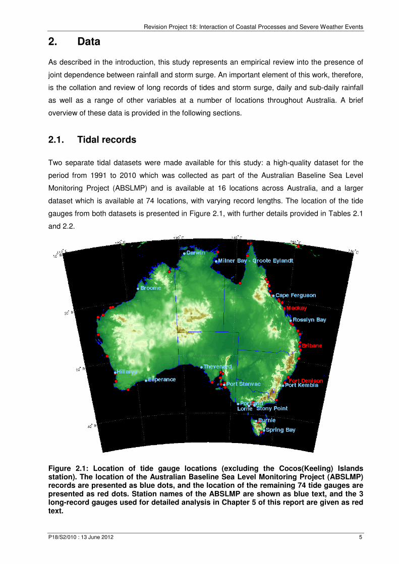
Two separate tidal datasets were made available for this study: a high-quality dataset for the
period from 1991 to 2010 which was collected as part of the Australian Baseline Sea Level
Monitoring Project (ABSLMP) and is available at 16 locations across Australia, and a larger
dataset which is available at 74 locations, with varying record lengths. The location of the tide
gauges from both datasets is presented in Figure 2.1, with further details provided in Tables 2.1
and 2.2.
Figure 2.1: Location of tide gauge locations (excluding the Cocos(Keeling) Islands station). The location of the Australian Baseline Sea Level Monitoring Project (ABSLMP) records are presented as blue dots, and the location of the remaining 74 tide gauges are presented as red dots. Station names of the ABSLMP are shown as blue text, and the 3 long-record gauges used for detailed analysis in Chapter 5 of this report are given as red text.

Revision Project 18: Interaction of Coastal Processes and Severe Weather Events
P18/S2/010 : 13 June 2012 6
Both datasets are available at an hourly resolution, with the ABSLMP record being based on six-
minute sea levels which were filtered with a cut-off of two hours and then decimated on the hour,
whereas the data from the other sites consisted of a combination of hourly point readings from
tide gauge traces and filtering from a range of other sampling intervals (personal
communication, Mr Paul Davill, National Tidal Centre, 4 March 2011).
Data from the 16 stations of the ABSLMP can be downloaded from
http://www.bom.gov.au/oceanography/projects/abslmp/data/index.shtml#table, with further
information on data formats, accuracy and other information provided there. Data from the 74
tide gauges maintained by various harbour and port authorities was collected by EngTest from
the National Tidal Centre (NTC), a division of the Bureau of Meteorology, and further information
on this dataset is available in the accompanying report (EngTest, 2010). These data are held
under licence from the relevant port and harbour authorities, and several qualifications have
been placed on its use. This includes the restriction that the data is to be used solely in the
context of the work of ARR Project 18, and that any changes to the scope of this work, including
commercialisation of tidal models, will require renegotiation of the licence agreements.
Furthermore, the relevant authorities have requested to be informed of the outcomes of Project
18. Further details on restrictions and qualifications is provided in (EngTest, 2010).
Each of the readings represent the total tidal level (referred to in the remainder of this report as
the ‘storm tide’), and which represents the combined influence of astronomical tides, storm
surges and other features such as tsunamis acting on the ocean. The component related to
astronomical tide is regular-periodic, and has been extracted from the storm tide record via a
harmonic analysis as described in Pugh (1987) and ((PCTMSL), 2007) using a total of 112 tidal
constituents (personal communication, Mr Paul Davill, National Tidal Centre, 4 March 2011).
The ‘residual’ component is the difference between the total tide level and the derived
astronomical tide, and thus by construction incorporates anything that is not regular-periodic.
This residual component will henceforth be referred to as the ‘storm surge’ component, which is
attributable to the combined influence of atmospheric pressure and wind anomalies acting on
the water body. It should be noted, however, that in certain cases where the tide gauge is
located at the mouth of a river, it is possible that catchment runoff also may be incorporated
within this storm surge component, and this may have a significant influence on the magnitude
of the estimation of the dependence between rainfall and storm surge. This will be discussed
further in Chapter 5.
Finally, in addition to information on astronomical tides and storm surges, the ABSLMP dataset
contains information on water temperature, air temperature, barometric pressure, and wind
speed and direction, which can be useful for a more detailed study into the behaviour of storm
Revision Project 18: Interaction of Coastal Processes and Severe Weather Events
P18/S2/010 : 13 June 2012 7
surges. Although this data was not used directly for the study described in this report, such data
may be useful for more in-depth scientific studies into the drivers of extreme storm surges in the
coastal zone.
Revision Project 18: Interaction of Coastal Processes and Severe Weather Events
P18/S2/010 : 13 June 2012 8
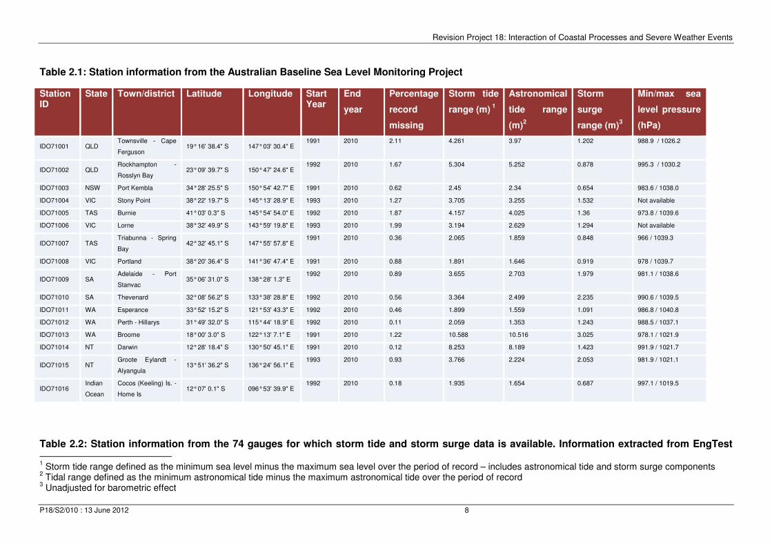
Table 2.1: Station information from the Australian Baseline Sea Level Monitoring Project
Station ID
State Town/district Latitude Longitude Start Year
End
year
Percentage
record
missing
Storm tide
range (m) 1
Astronomical
tide range
(m)2
Storm
surge
range (m)3
Min/max sea
level pressure
(hPa)
IDO71001 QLD Townsville - Cape
Ferguson 19° 16' 38.4" S 147° 03' 30.4" E
1991 2010 2.11 4.261 3.97 1.202 988.9 / 1026.2
IDO71002 QLD Rockhampton -
Rosslyn Bay 23° 09' 39.7" S 150° 47' 24.6" E
1992 2010 1.67 5.304 5.252 0.878 995.3 / 1030.2
IDO71003 NSW Port Kembla 34° 28' 25.5" S 150° 54' 42.7" E 1991 2010 0.62 2.45 2.34 0.654 983.6 / 1038.0
IDO71004 VIC Stony Point 38° 22' 19.7" S 145° 13' 28.9" E 1993 2010 1.27 3.705 3.255 1.532 Not available
IDO71005 TAS Burnie 41° 03' 0.3" S 145° 54' 54.0" E 1992 2010 1.87 4.157 4.025 1.36 973.8 / 1039.6
IDO71006 VIC Lorne 38° 32' 49.9" S 143° 59' 19.8" E 1993 2010 1.99 3.194 2.629 1.294 Not available
IDO71007 TAS Triabunna - Spring
Bay 42° 32' 45.1" S 147° 55' 57.8" E
1991 2010 0.36 2.065 1.859 0.848 966 / 1039.3
IDO71008 VIC Portland 38° 20' 36.4" S 141° 36' 47.4" E 1991 2010 0.88 1.891 1.646 0.919 978 / 1039.7
IDO71009 SA Adelaide - Port
Stanvac 35° 06' 31.0" S 138° 28' 1.3" E
1992 2010 0.89 3.655 2.703 1.979 981.1 / 1038.6
IDO71010 SA Thevenard 32° 08' 56.2" S 133° 38' 28.8" E 1992 2010 0.56 3.364 2.499 2.235 990.6 / 1039.5
IDO71011 WA Esperance 33° 52' 15.2" S 121° 53' 43.3" E 1992 2010 0.46 1.899 1.559 1.091 986.8 / 1040.8
IDO71012 WA Perth - Hillarys 31° 49' 32.0" S 115° 44' 18.9" E 1992 2010 0.11 2.059 1.353 1.243 988.5 / 1037.1
IDO71013 WA Broome 18° 00' 3.0" S 122° 13' 7.1" E 1991 2010 1.22 10.588 10.516 3.025 978.1 / 1021.9
IDO71014 NT Darwin 12° 28' 18.4" S 130° 50' 45.1" E 1991 2010 0.12 8.253 8.189 1.423 991.9 / 1021.7
IDO71015 NT Groote Eylandt -
Alyangula 13° 51' 36.2" S 136° 24' 56.1" E
1993 2010 0.93 3.766 2.224 2.053 981.9 / 1021.1
IDO71016 Indian
Ocean
Cocos (Keeling) Is. -
Home Is 12° 07' 0.1" S 096° 53' 39.9" E
1992 2010 0.18 1.935 1.654 0.687 997.1 / 1019.5
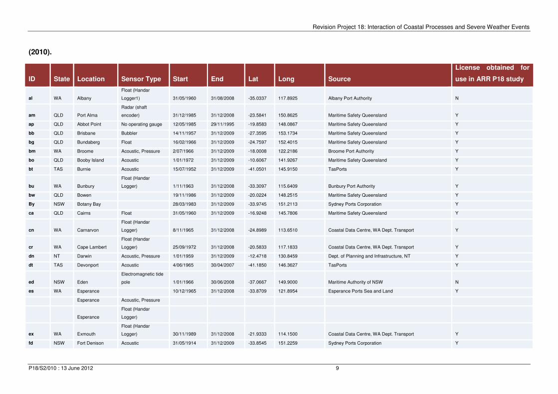
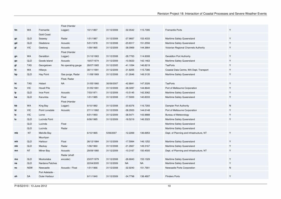
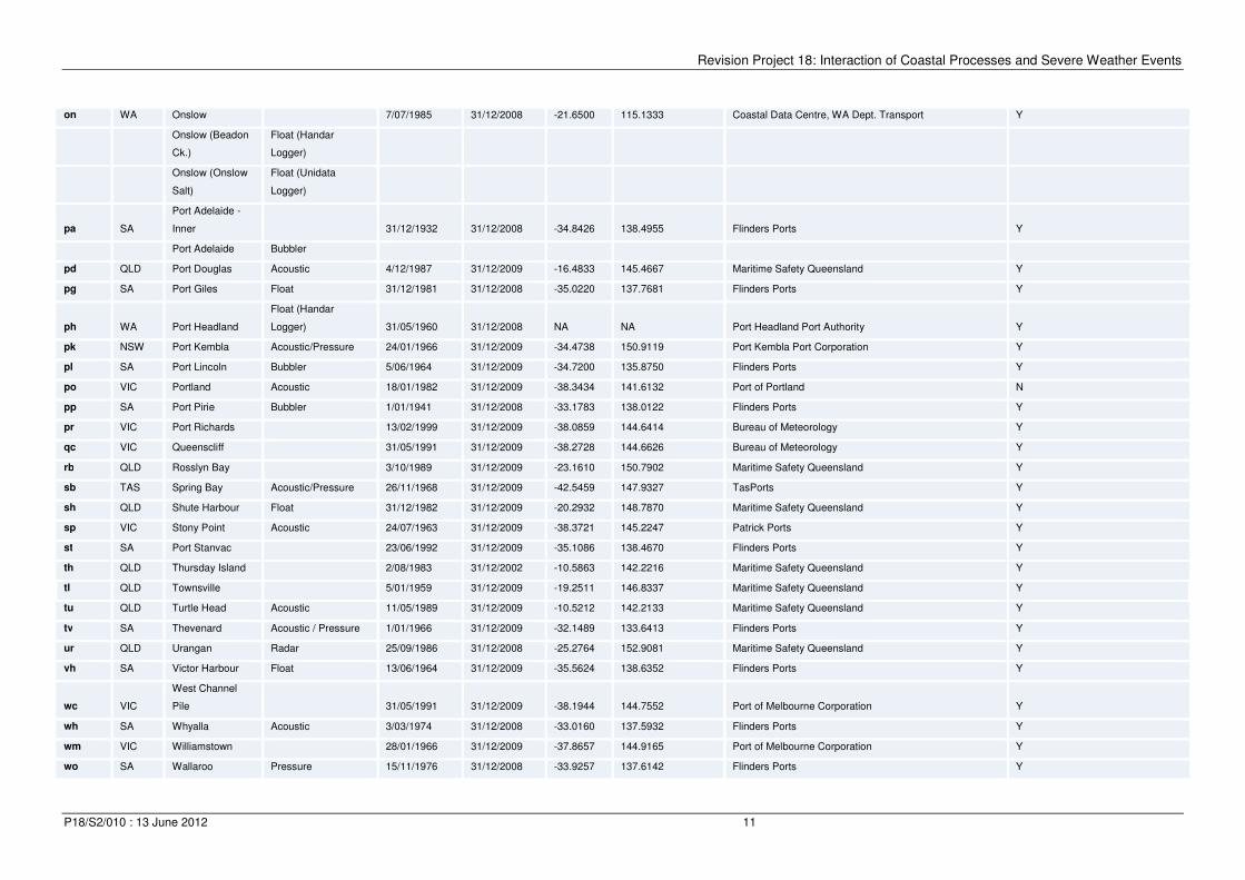
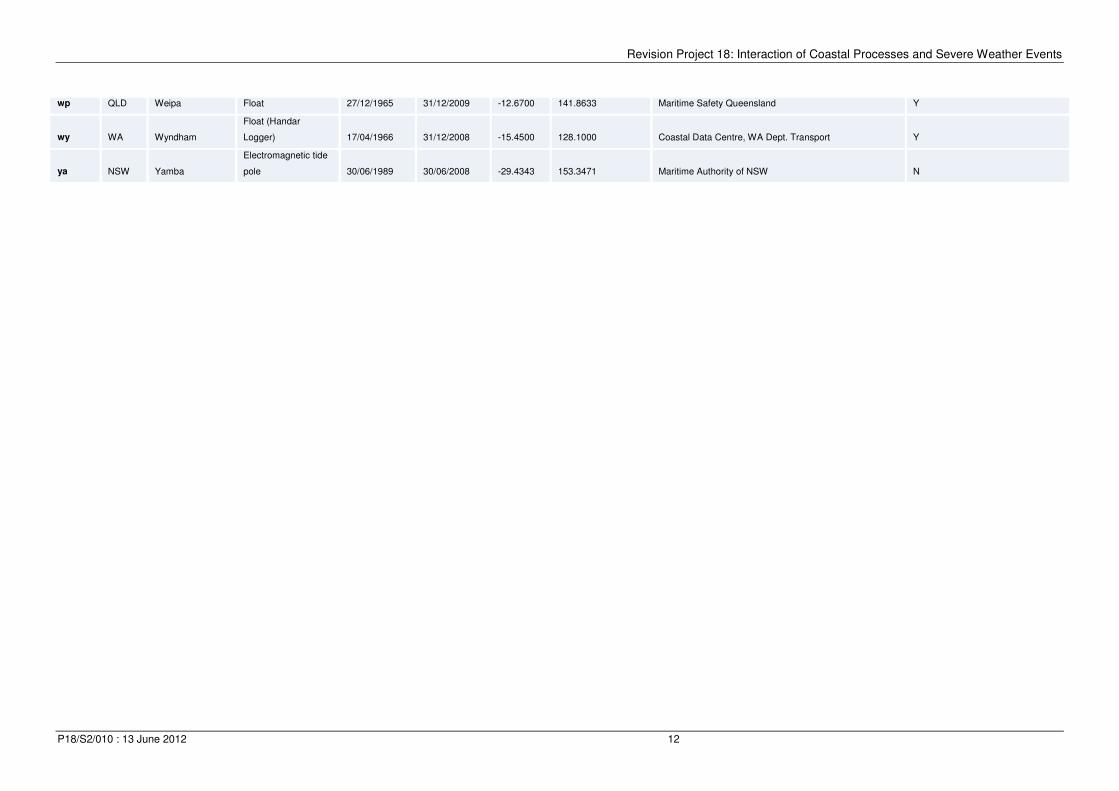
Table 2.2: Station information from the 74 gauges for which storm tide and storm surge data is available. Information extracted from EngTest 1 Storm tide range defined as the minimum sea level minus the maximum sea level over the period of record – includes astronomical tide and storm surge components
2 Tidal range defined as the minimum astronomical tide minus the maximum astronomical tide over the period of record
3 Unadjusted for barometric effect
Revision Project 18: Interaction of Coastal Processes and Severe Weather Events
P18/S2/010 : 13 June 2012 9
(2010).
ID State Location Sensor Type Start End Lat Long Source
License obtained for
use in ARR P18 study
al WA Albany
Float (Handar
Logger1) 31/05/1960 31/08/2008 -35.0337 117.8925 Albany Port Authority N
am QLD Port Alma
Radar (shaft
encoder) 31/12/1985 31/12/2008 -23.5841 150.8625 Maritime Safety Queensland Y
ap QLD Abbot Point No operating gauge 12/05/1985 29/11/1995 -19.8583 148.0867 Maritime Safety Queensland Y
bb QLD Brisbane Bubbler 14/11/1957 31/12/2009 -27.3595 153.1734 Maritime Safety Queensland Y
bg QLD Bundaberg Float 16/02/1966 31/12/2009 -24.7597 152.4015 Maritime Safety Queensland Y
bm WA Broome Acoustic, Pressure 2/07/1966 31/12/2009 -18.0008 122.2186 Broome Port Authority Y
bo QLD Booby Island Acoustic 1/01/1972 31/12/2009 -10.6067 141.9267 Maritime Safety Queensland Y
bt TAS Burnie Acoustic 15/07/1952 31/12/2009 -41.0501 145.9150 TasPorts Y
bu WA Bunbury
Float (Handar
Logger) 1/11/1963 31/12/2008 -33.3097 115.6409 Bunbury Port Authority Y
bw QLD Bowen 19/11/1986 31/12/2009 -20.0224 148.2515 Maritime Safety Queensland Y
By NSW Botany Bay 28/03/1983 31/12/2009 -33.9745 151.2113 Sydney Ports Corporation Y
ca QLD Cairns Float 31/05/1960 31/12/2009 -16.9248 145.7806 Maritime Safety Queensland Y
cn WA Carnarvon
Float (Handar
Logger) 8/11/1965 31/12/2008 -24.8989 113.6510 Coastal Data Centre, WA Dept. Transport Y
cr WA Cape Lambert
Float (Handar
Logger) 25/09/1972 31/12/2008 -20.5833 117.1833 Coastal Data Centre, WA Dept. Transport Y
dn NT Darwin Acoustic, Pressure 1/01/1959 31/12/2009 -12.4718 130.8459 Dept. of Planning and Infrastructure, NT Y
dt TAS Devonport Acoustic 4/06/1965 30/04/2007 -41.1850 146.3627 TasPorts Y
ed NSW Eden
Electromagnetic tide
pole 1/01/1966 30/06/2008 -37.0667 149.9000 Maritime Authority of NSW N
es WA Esperance 10/12/1965 31/12/2008 -33.8709 121.8954 Esperance Ports Sea and Land Y
Esperance Acoustic, Pressure
Esperance
Float (Handar
Logger)
ex WA Exmouth
Float (Handar
Logger) 30/11/1989 31/12/2008 -21.9333 114.1500 Coastal Data Centre, WA Dept. Transport Y
fd NSW Fort Denison Acoustic 31/05/1914 31/12/2009 -33.8545 151.2259 Sydney Ports Corporation Y
Revision Project 18: Interaction of Coastal Processes and Severe Weather Events
P18/S2/010 : 13 June 2012 10
fm WA Fremantle
Float (Handar
Logger) 10/1/1897 31/12/2009 -32.0542 115.7395 Fremantle Ports Y
gc QLD
Gold Coast
Seaway Radar 1/01/1987 31/12/2009 -27.9667 153.4333 Maritime Safety Queensland Y
gd QLD Gladstone Acoustic 5/01/1978 31/12/2008 -23.8317 151.2556 Maritime Safety Queensland Y
gl VIC Geelong Acoustic 1/09/1965 31/12/2009 -38.0969 144.3864 Victorian Regional Channels Authority Y
gn WA Geraldton
Float (Handar
Logger) 31/10/1963 31/12/2008 -28.7763 114.6008 Geraldton Port Authority Y
go QLD Goods Island Acoustic 18/07/1974 31/12/2009 -10.5633 142.1463 Maritime Safety Queensland Y
gt TAS Georgetown No operating gauge 28/07/1965 31/12/2005 -41.1094 146.8219 TasPorts Y
hi WA Hillarys 30/11/1991 31/12/2009 -31.8255 115.7386 Coastal Data Centre, WA Dept. Transport Y
hp QLD Hay Point Gas purge, Radar 11/08/1969 31/12/2008 -21.2646 149.3135 Maritime Safety Queensland Y
Float, Radar
ht TAS Hobart NA 31/05/1960 30/09/2007 -42.8841 147.3326 TasPorts Y
hv VIC Hovell Pile 31/05/1991 31/12/2009 -38.3287 144.8640 Port of Melbourne Corporation Y
ip QLD Ince Point Acoustic 7/03/1971 31/12/2009 -10.5145 142.3062 Maritime Safety Queensland Y
ka QLD Karumba Float 1/01/1985 31/12/2008 -17.5000 140.8333 Maritime Safety Queensland Y
kb WA King Bay
Float (Handar
Logger) 9/10/1982 31/12/2008 -20.6376 116.7293 Dampier Port Authority N
ld VIC Point Lonsdale Acoustic 27/11/1962 31/12/2009 -38.2933 144.6148 Port of Melbourne Corporation Y
lo VIC Lorne 6/01/1993 31/12/2009 -38.5471 143.9888 Bureau of Meteorology Y
lu QLD Lucinda Point 6/06/1985 31/12/2009 -18.5219 146.3323 Maritime Safety Queensland Y
QLD Lucinda Float Maritime Safety Queensland
QLD Lucinda Radar Maritime Safety Queensland
mb NT Melville Bay 6/10/1965 5/08/2007 -12.2269 136.6953 Dept. of Planning and Infrastructure, NT Y
mh QLD
Mourilyan
Harbour Float 26/12/1984 31/12/2009 -17.5994 146.1252 Maritime Safety Queensland Y
mk QLD Mackay Radar 1/06/1960 31/12/2008 -21.2667 149.3167 Maritime Safety Queensland Y
mn NT Milner Bay Acoustic 29/09/1980 31/12/2009 -10.3167 150.4500 Dept. of Planning and Infrastructure, NT Y
mo QLD Mooloolaba
Radar (shaft
encoder) 23/07/1979 31/12/2008 -26.6843 153.1329 Maritime Safety Queensland Y
na QLD Nardana Patches 22/04/2005 31/12/2009 NA NA Maritime Safety Queensland Y
nc NSW Newcastle Acoustic / Float 1/01/1966 31/12/2008 -32.9240 151.7901 Newcastle Ports Corporation N
oh SA
Port Adelaide -
Outer Harbour 9/11/1940 31/12/2009 -34.7798 138.4807 Flinders Ports Y
Revision Project 18: Interaction of Coastal Processes and Severe Weather Events
P18/S2/010 : 13 June 2012 11
on WA Onslow 7/07/1985 31/12/2008 -21.6500 115.1333 Coastal Data Centre, WA Dept. Transport Y
Onslow (Beadon
Ck.)
Float (Handar
Logger)
Onslow (Onslow
Salt)
Float (Unidata
Logger)
pa SA
Port Adelaide -
Inner 31/12/1932 31/12/2008 -34.8426 138.4955 Flinders Ports Y
Port Adelaide Bubbler
pd QLD Port Douglas Acoustic 4/12/1987 31/12/2009 -16.4833 145.4667 Maritime Safety Queensland Y
pg SA Port Giles Float 31/12/1981 31/12/2008 -35.0220 137.7681 Flinders Ports Y
ph WA Port Headland
Float (Handar
Logger) 31/05/1960 31/12/2008 NA NA Port Headland Port Authority Y
pk NSW Port Kembla Acoustic/Pressure 24/01/1966 31/12/2009 -34.4738 150.9119 Port Kembla Port Corporation Y
pl SA Port Lincoln Bubbler 5/06/1964 31/12/2009 -34.7200 135.8750 Flinders Ports Y
po VIC Portland Acoustic 18/01/1982 31/12/2009 -38.3434 141.6132 Port of Portland N
pp SA Port Pirie Bubbler 1/01/1941 31/12/2008 -33.1783 138.0122 Flinders Ports Y
pr VIC Port Richards 13/02/1999 31/12/2009 -38.0859 144.6414 Bureau of Meteorology Y
qc VIC Queenscliff 31/05/1991 31/12/2009 -38.2728 144.6626 Bureau of Meteorology Y
rb QLD Rosslyn Bay 3/10/1989 31/12/2009 -23.1610 150.7902 Maritime Safety Queensland Y
sb TAS Spring Bay Acoustic/Pressure 26/11/1968 31/12/2009 -42.5459 147.9327 TasPorts Y
sh QLD Shute Harbour Float 31/12/1982 31/12/2009 -20.2932 148.7870 Maritime Safety Queensland Y
sp VIC Stony Point Acoustic 24/07/1963 31/12/2009 -38.3721 145.2247 Patrick Ports Y
st SA Port Stanvac 23/06/1992 31/12/2009 -35.1086 138.4670 Flinders Ports Y
th QLD Thursday Island 2/08/1983 31/12/2002 -10.5863 142.2216 Maritime Safety Queensland Y
tl QLD Townsville 5/01/1959 31/12/2009 -19.2511 146.8337 Maritime Safety Queensland Y
tu QLD Turtle Head Acoustic 11/05/1989 31/12/2009 -10.5212 142.2133 Maritime Safety Queensland Y
tv SA Thevenard Acoustic / Pressure 1/01/1966 31/12/2009 -32.1489 133.6413 Flinders Ports Y
ur QLD Urangan Radar 25/09/1986 31/12/2008 -25.2764 152.9081 Maritime Safety Queensland Y
vh SA Victor Harbour Float 13/06/1964 31/12/2009 -35.5624 138.6352 Flinders Ports Y
wc VIC
West Channel
Pile 31/05/1991 31/12/2009 -38.1944 144.7552 Port of Melbourne Corporation Y
wh SA Whyalla Acoustic 3/03/1974 31/12/2008 -33.0160 137.5932 Flinders Ports Y
wm VIC Williamstown 28/01/1966 31/12/2009 -37.8657 144.9165 Port of Melbourne Corporation Y
wo SA Wallaroo Pressure 15/11/1976 31/12/2008 -33.9257 137.6142 Flinders Ports Y
Revision Project 18: Interaction of Coastal Processes and Severe Weather Events
P18/S2/010 : 13 June 2012 12
wp QLD Weipa Float 27/12/1965 31/12/2009 -12.6700 141.8633 Maritime Safety Queensland Y
wy WA Wyndham
Float (Handar
Logger) 17/04/1966 31/12/2008 -15.4500 128.1000 Coastal Data Centre, WA Dept. Transport Y
ya NSW Yamba
Electromagnetic tide
pole 30/06/1989 30/06/2008 -29.4343 153.3471 Maritime Authority of NSW N
Revision Project 18: Interaction of Coastal Processes and Severe Weather Events
P18/S2/010 : 13 June 2012 13
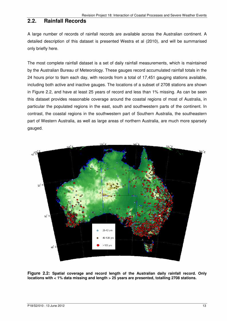
2.2. Rainfall Records
A large number of records of rainfall records are available across the Australian continent. A
detailed description of this dataset is presented Westra et al (2010), and will be summarised
only briefly here.
The most complete rainfall dataset is a set of daily rainfall measurements, which is maintained
by the Australian Bureau of Meteorology. These gauges record accumulated rainfall totals in the
24 hours prior to 9am each day, with records from a total of 17,451 gauging stations available,
including both active and inactive gauges. The locations of a subset of 2708 stations are shown
in Figure 2.2, and have at least 25 years of record and less than 1% missing. As can be seen
this dataset provides reasonable coverage around the coastal regions of most of Australia, in
particular the populated regions in the east, south and southwestern parts of the continent. In
contrast, the coastal regions in the southwestern part of Southern Australia, the southeastern
part of Western Australia, as well as large areas of northern Australia, are much more sparsely
gauged.
Figure 2.2: Spatial coverage and record length of the Australian daily rainfall record. Only locations with < 1% data missing and length > 25 years are presented, totalling 2708 stations.
Revision Project
P18/S2/010 : 13 June 2012
Although the daily dataset generally provides reasonable coverage of long, high
data, and is particularly useful
seasonal, annual or longer rainfall, the exact
recorded. For this information it is necessary to use the sub
collected using a combination of Dines pluviographs, Tipping Bucket Rain Gauges and other
instruments and which are able to
This record is also available from the Australian Bureau of Meteorology, and information on the
spatial location as well as the
gauging density is much sparser
locations with records extending back prior to the 1960s. Nevertheless
most populated areas along the coastal zone, particularly along t
Australian coastline, is reasonable.
Figure 2.3: Spatial coverage and record length of the Australian sub
record.
Revision Project 18: Interaction of Coastal Processes and Severe Weather Events
Although the daily dataset generally provides reasonable coverage of long, high
data, and is particularly useful for providing information on the properties of aggregated daily,
seasonal, annual or longer rainfall, the exact sub-temporal distribution of the rainfall is not
recorded. For this information it is necessary to use the sub-daily rainfall record,
collected using a combination of Dines pluviographs, Tipping Bucket Rain Gauges and other
are able to record rainfall at very fine sub-hourly temporal resolutions.
This record is also available from the Australian Bureau of Meteorology, and information on the
spatial location as well as the record length is summarised in Figure 2.3
gauging density is much sparser compared with the daily dataset, and there are very few
locations with records extending back prior to the 1960s. Nevertheless,
most populated areas along the coastal zone, particularly along the eastern and southeastern
Australian coastline, is reasonable.
: Spatial coverage and record length of the Australian sub
18: Interaction of Coastal Processes and Severe Weather Events
14
Although the daily dataset generally provides reasonable coverage of long, high-quality rainfall
information on the properties of aggregated daily,
temporal distribution of the rainfall is not
daily rainfall record, which is
collected using a combination of Dines pluviographs, Tipping Bucket Rain Gauges and other
hourly temporal resolutions.
This record is also available from the Australian Bureau of Meteorology, and information on the
2.3. As can be seen the
compared with the daily dataset, and there are very few
gauging density in the
he eastern and southeastern
: Spatial coverage and record length of the Australian sub-daily pluviograph
Revision Project 18: Interaction of Coastal Processes and Severe Weather Events
P18/S2/010 : 13 June 2012 15
2.3. Additional data
There are numerous additional datasets which can be used to derive a better understanding of
the nature extreme rainfall and storm surges in the coastal zone. Although these datasets were
not used in the present study, an important element of this pilot study is to review the data which
can be used to inform further and more in-depth studies in the future, and therefore a brief
overview will be given here.
Extreme rainfall and storm surge are both driven by atmospheric anomalies, and therefore
information on the state of the atmosphere during extreme events provides useful information
into the physical mechanisms by which such extremes occur. Historical data is typically
available as point measurements taken at regular intervals of ground-level atmospheric variable
such as sea level pressure, temperature and wind strength and direction, with near-complete
records of each of these variables being available as part of the ABSLMP record at 16 locations
throughout Australia. An alternative source of information on the historical atmosphere is
obtained from reanalysis datasets, which are datasets which assimilate ground and upper-
atmospheric data into an atmospheric climate model, in order to estimate a three-dimensional
representation of a range of measurable and non-measurable atmospheric fields. Examples of
such reanalysis datasets include the NCEP/NCAR reanalysis (Kalnay et al., 1996), the
European ERA-40 and ERA-Interim reanalyses (Uppala et al., 2006), the Japanese reanalysis
dataset (JRA25; Onogi et al., 2007) and a very recent higher spatial and temporal resolution
update of the NCEP reanalysis referred to as the NCEP Climate Forecast Systems Reanalysis
(CFSR; Saha et al., 2010). Such records are widely used for classifying different synoptic
systems, and therefore may be useful for any study which looks at the synoptic conditions that
drive simultaneous extreme rainfall and flooding, as well as conditions when only extreme
rainfall can be expected to occur in the absence of extreme storm surge, or vice versa.
Along similar lines, there are historical accounts of different extreme storms which can be used
to supplement the instrumental data. For example, Callaghan and Helman (2008) documented
severe storms on the east coast of Australia from 1770 to 2008, from Cape York to Tasmania,
using a range of documentary sources ranging from historical accounts in maritime records in
the early parts of the record through to Bureau of Meteorology and newspaper accounts from
the 1900’s onwards. Furthermore, information is available on cyclone tracks from the Joint
Typhoon Warning Centre (http://www.usno.navy.mil/JTWC/) or from the Australian Bureau of
Meteorology (http://www.bom.gov.au/cyclone/history/index.shtml), and may be useful to
characterise extreme rainfall and storm surge that are specifically attributable to tropical
cyclones.
Finally, work is currently underway by the CSIRO (Abbs and McInnes, 2010) on the interaction
Revision Project 18: Interaction of Coastal Processes and Severe Weather Events
P18/S2/010 : 13 June 2012 16
between extreme rainfall and storm surge under future climate conditions. This is achieved by
synoptic classification of large events using the ERA-40 and ERA-interim reanalyses for current
climate conditions, and then using the CSIRO Conformal-Cubic Atmospheric Model (CCAM)
forced to a GCM-derived bias-corrected sea surface temperature field for future climate
conditions. This study projects increases in coincident events in southwestern Australia
(including Fremantle and Esperance) due to increased occurrence of closed low systems, with
little change or a decrease in coincident rainfall and sea level events for eastern coastline south
of Brisbane. Quantitative assessments of the implications of this on flood risk, however, are
currently unavailable.

Revision Project 18: Interaction of Coastal Processes and Severe Weather Events
P18/S2/010 : 13 June 2012 17
3. Methodology
The second objective of this pilot study is to identify a suitable statistical methodology to
represent this dependence. The ultimate application of such a methodology is the estimation of
design flood quantiles such as peak flows or flood levels, which are often required at
magnitudes greater than the largest event that has been observed in the instrumental record. As
such, the identified methodology must: (a) accurately simulate the dependence between the
observed rainfall and storm surge data; (b) be suitable for the estimation of flood quantiles when
they result from multiple distinct physical processes; and (c) have a theoretically sound basis for
extrapolation beyond the largest recorded event. As the objective of this study is to identify a
methodology that can be included in the Australian Rainfall and Runoff flood estimation
guidelines, any such methodology will also need to be have a sound theoretical basis and be
well supported by the peer-reviewed statistical literature, while still being relatively simply to
apply by the practicing engineering community.
The approach that was selected is derived from the family of bivariate extreme value
distributions as described in Coles (2001) together with a number of additional references that
will be summarised in this section. The principal advantages of the extreme value approaches
lies in their asymptotic justification, in which the maxima Mn of a set of independent random
variables {X1,..., Xn} as � → ∞ will converge to a single family of distributions collectively known
as the Generalised Extreme Value (GEV) distribution (Coles, 2001; Fisher and Tippett, 1928;
Gnedenko, 1943; Katz et al., 2002; Kotz and Nadarajah, 2000). Although theoretically this
justification applies only in the limit as � → ∞, in practise extreme value models have been used
successfully to a wide variety of real world problems, including the statistical modelling of
extreme rainfall (Koutsoyiannis, 2004), floods (Davison and Smith, 1990; Katz et al., 2002;
Ribatet et al., 2009) and storm surges (Bernardara et al., 2011). Furthermore, the univariate
version of the GEV distribution is already being supported in other parts of the forthcoming
Australian Rainfall and Runoff guidelines, including the draft chapter on the estimation of peak
discharge (Australian Rainfall and Runoff, 2006), and thus is likely to be familiar to a large part
of the practicing engineering community. Finally, a conceptually simple approach for estimating
design parameters such as design floods when they are resulting from multiple distinct physical
processes (henceforth termed ‘constituent variables’) has been derived by Coles and Tawn
(1994), and will form the theoretical basis for much of the methodology described here.
The remainder of this chapter will be structured as follows. In the following section, a brief
overview will be provided of univariate probability concepts and univariate extreme value theory,
laying the foundation for the remainder of the chapter. This will be followed by four conceptual
approaches for modelling bivariate extremes, including component-wise maxima, threshold-
Revision Project 18: Interaction of Coastal Processes and Severe Weather Events
P18/S2/010 : 13 June 2012 18
excess and point process techniques for simulating bivariate distributions, as well as a structure
variable approach which involves translating the bivariate distribution into a univariate process
prior to the application of univariate extreme value models. Finally, a brief review of a number of
additional issues, including the accounting of temporal dependence and simulating the
implications of climate change, will be discussed. The treatment presented in this section is
largely based on that of Coles (2001), and the nomenclature used here has followed this
reference where possible.
3.1. Brief Overview of Univariate Extreme Value Theory
Extreme value theory concerns the statistical behaviour of the maxima (or equivalently, the
minima) of a set of n independent random variables X1,..., Xn with common distribution function
F:
Mn = max{X1,..., Xn} (3.1)
In particular, as � → ∞, the distribution of (Mn – bn) / an, for suitably chosen constants {an>0} and
{bn} will converge to a family of models collectively known as the generalised extreme value
(GEV) distribution. In this way extreme value theory is the extreme values analogue to the
central limit theorem for the sample mean, in which the mean of a sample converges to a normal
distribution for large n, for a large range of original distribution functions F. This is the attraction
of using extreme value distributions to simulate extremes of processes such as rainfall, floods or
storm surge: regardless of the statistical characteristics of the original process, the statistical
behaviour of the most extreme values of this process can be expected to follow a GEV
distribution, provided that the values of X are independent and identically distributed4, and that
the choice of n is sufficiently high.
The distribution function of the GEV distribution is given as:
���� = �� �− �1 + � ����� ����/�� (3.2)
where −∞ < � < ∞ is known as the location parameter, � > 0 is known as the scale parameter,
and −∞ < � < ∞ is known as the shape parameter. Here and in the remainder of this report, F()
and f() represent arbitrary distribution and density functions, respectively, whereas G() and g()
represent the extreme value distribution and density functions specifically. The forms of the GEV
4 This assumption is not strictly necessary, as extreme value approaches have also been developed for
stationary distributions that are dependent in time, as well as non-stationary distributions; see Coles S.G. (2001) An Introduction to Statistical Modelling of Extreme Values Springer, London.

Revision Project 18: Interaction of Coastal Processes and Severe Weather Events
P18/S2/010 : 13 June 2012 19
include the Fréchet and Weibull distributions, for which � > 0 and � < 0, respectively, and the
Gumbel distribution which is defined in the limit as � → 0. The estimation of model parameters,
given the data, can be achieved variously through the method of moments, the method of L-
moments (Hosking et al., 1985), maximum likelihood (Coles, 2001) or via Bayesian techniques
(Coles and Powell, 1996), with the method of maximum likelihood used as the estimation
method for the remainder of this report.
The form of extreme value model given in equation 3.2 is often referred to as a block maxima
model, as it is defined over a block of n values of X. When the block size is set to a year, the
model becomes an annual maximum model, with this being a common representation for a
range of environmental processes. In doing so it is implicitly assumed that this value of n is
sufficiently large such that the asymptotic properties of the extreme value theorem will hold
approximately, whereas in practice other distributions such as the log-Pearson III and log-
normal distributions sometimes provide better fits to some datasets (Australian Rainfall and
Runoff, 2006). The remainder of this report will nevertheless focus on the family of extreme
value distributions, however it should be noted that the recommended methodology for
addressing bivariate extremes addresses the marginal distribution of the constituent processes
separately from their joint distribution, and thus for practical applications it is possible to use
distributions other than the GEV distribution for modelling each marginal distribution.
An alternative model formulation to the block maximum model described above is the threshold
model (often referred to as a peak over thresholds (POT) model in the hydrological literature), in
which all the events Xi whose value exceeds a sufficiently high threshold u are classified as
‘extreme’ (e.g. Davison and Smith, 1990). In this case, the distribution function of (X – u) follows
a generalised Pareto distribution (GPD), and is given as:
Pr{% > �|% > '} = �1 + ����)��* ���/� (3.3)
and thus
G�x� = 1 − -) �1 + ����)��* ���/� (3.4)
where -) = Pr{% > '} and �. is the scale parameter for the threshold excess model, and relates
to the scale parameter from the GEV model via:
�. = � + ��' − �� (3.5)
Revision Project 18: Interaction of Coastal Processes and Severe Weather Events
P18/S2/010 : 13 June 2012 20
An important consideration in developing the threshold excess model is the choice of suitable
threshold, with this choice effectively representing a trade-off between bias and variance. In
particular if the threshold is too low, then the parameters will be estimated more precisely due to
the large amount of data available, but will most likely also be biased as the asymptotic
justification of the extreme value model will not be valid even as an approximation. Conversely,
if the threshold is too high then it will be more likely that the extreme value model will provide a
reasonable approximation to the data, but the limited sample size will mean that the parameter
estimates are highly variable and thus imprecise.
One diagnostic to evaluate whether an appropriate threshold value is selected is known as the
mean residual life plot. The basis for this diagnostic is as follows. Assuming the excesses (X-u0)
above a given threshold u0 conforms to a generalised Pareto distribution, then the expected
value of these excesses is given as:
/�% − '0|% > '0� = �12��� (3.6)
provided � < 1, where �)2 is used to denote the scale parameter corresponding to the excesses
over the threshold '0. If the generalised Pareto distribution was valid for all excesses above '0, it must also be valid for all thresholds ' > '0:
/�% − '|% > '� = �1��� = �12341��� (3.7)
with the second part of this equation derived from Equation 3.5. As a result of the above,
provided that the choice of '0 follows a generalised Pareto distribution, the expectation of (X-u),
given as:
�51∑ ���7� − '�5178� ∶ ' < �:;� (3.8)
where x(1),..., x(nu) represents the nu observations that exceed u, and this relationship should
change as a linear function of u. The mean residual life plot is simply a plot of the left hand side
of Equation 3.8 against u, with the critical threshold being the point at which the plot becomes
linear.
The second approach suggests that above the critical threshold, estimates of the shape
parameter � should be constant, while estimates of the �) should change linearly as a function
of u. Both these plots are used as diagnostics in checking the threshold selection, and are
Revision Project 18: Interaction of Coastal Processes and Severe Weather Events
P18/S2/010 : 13 June 2012 21
described further in Chapter 4.
3.2. Modelling Dependence of Bivariate Extremes
Analogous to univariate extreme value approaches, there are at least three ways of
characterising multivariate extremes: component-wise block maxima, threshold-excess and
point processes. A fourth characterisation involves developing a structure function to translate
the multivariate model to a univariate model, and is discussed briefly in the final section. Once
again the treatment largely follows the treatment in Coles (2001), although additional references
are provided where appropriate and some changes in nomenclature have been made to ensure
consistency with later sections.
To simplify the discussion, all the theory that follows will be in terms of bivariate distributions,
although higher-dimensional generalisations are usually available. Unfortunately, even in the
case of bivariate distributions there are a number of difficulties that arise in fitting and
interpreting these distributions compared to their univariate analogues. These are discussed
where appropriate, and methods to account for these difficulties are outlined where possible.
3.2.1. Component-wise block maxima approach
Firstly consider the block maxima approach. The bivariate models considered here are focus on
the distribution of bivariate block maxima, defined as:
<5 = �=�,5,=?,5� (3.9)
where
=�,5 = max78�,…,5{%7}
=?,5 = max78�,…,5{C7}
Here, Mn is referred to as the vector of componentwise maxima. To simplify the subsequent
description, we assume that Xi and Yi are random variables with unit Fréchet margins5 and
therefore can be described via the distribution function D�E� = exp�−1/E�, corresponding to a 5 Some publications and software packages, such as the evd software package, used for part of the
analysis in this report assumes unit exponential margins given by G(z) = exp(-z) rather than unit Fréchet margins described here. Another popular choice is transforming the data via the distribution function to a unit hypercube [0,1]
d, in which case the dependence function is known as a copula, C. All cases require
transformation of the marginal distributions to some standardised form, often via a univariate extreme value distribution, prior to fitting the relevant joint distribution function. As such, information used for characterising the marginal distributions of each variable is considered separately to information on the dependence between the variables. Options for estimating the likelihood of the marginal and joint distributions simultaneously also exist, but have not been implemented here.

Revision Project 18: Interaction of Coastal Processes and Severe Weather Events
P18/S2/010 : 13 June 2012 22
GEV distribution of Equation 3.2 with parameters � = 1, � = 1 and � = 1. Furthermore,
analogous to the univariate situation, the maxima are rescaled via <5∗ = �=�,5/�,=?,5/��. Then
as � → ∞, under a wide range of conditions it can be shown that the bivariate extreme value
distribution G(x,y) has the form:
���, J� = exp{−K��, J�} ,� > 0, J > 0 (3.10)
where
K��, J� = 2M max �N� , ��N? ��0 OP�Q� (3.11)
satisfying constraint:
M QOP�Q� = 1/2�0 (3.12)
where V is referred to as the exponent measure function, H is a non-negative measure, and w is
the angular component of x and y defined over [0,1], as will be discussed further in Section
3.2.3. If H is differentiable with density h, Equation 3.11 becomes:
K��, J� = 2M max �N� , ��N? ��0 ℎ�Q�OQ (3.13)
Although these results are described assuming unit-Fréchet margins, this implies no loss of
generality as any GEV distribution can be transformed to the unit Fréchet scale via:
E = �1 + � �T��� ���/� (3.14)
Thus, one can write the bivariate GEV distribution for the full class of GEV marginal distributions
as follows:
���, J� = exp{−K��., J.�} (3.15)
The above formulation gives a complete characterisation of bivariate extreme value
distributions, however it leads to a very wide class of possible distributions, with any distribution
function of H satisfying Equation 3.12 being admissible. A specific example of such a bivariate
extreme value distribution is the logistic model (Tawn, 1988):
Revision Project 18: Interaction of Coastal Processes and Severe Weather Events
P18/S2/010 : 13 June 2012 23
���, J� = ��U−V���/W + J��/WXWY0 < Z ≤ 1 (3.16)
Independence is obtained when α = 1, and complete dependence is obtained when α = 0. The
density function describing the dependence is given by:
ℎ�Q� = �\ �Z�� − 1�{Q�1 − Q�}����/W{Q��/W + �1 − Q���/W}W�\ (3.17)
This simply represents a one-parameter dependence model fitted to the angular component (w)
of the unit-Fréchet-transformed data above the minimum threshold rmin, such that a total of
seven parameters must be estimated (three for each marginal transformation from GEV to unit-
Fréchet, and a single dependence parameter α).
The limitation of the use of componentwise maxima is that the Mx,n and My,n need not occur
simultaneously, and therefore Mn will in general not correspond to a combination of Mx,n and My,n
which have actually co-occurred. In fact, as X and Y become increasingly mutually independent,
the probability of the sequence of maxima co-occurring usually will become increasingly low,
with for example the annual maximum daily rainfall expected to occur on the same day as the
annual maximum daily storm surge on average only once in every 365 years assuming
complete independence and ignoring seasonal effects. Thus, for applications such as flood
estimation where the question of whether the extreme storm surge event and the extreme
rainfall event will occur simultaneously will have a large bearing on the results, the simulation of
componentwise maxima will not provide the necessary information. Fortunately, much of the
theory developed above applies equally to the class of threshold-excess and point process
models, with both classes focusing on simulating events which occur simultaneously in time.
3.2.2. Threshold excess approach
The univariate representation of the threshold-excess model was provided in Equation 3.3.
Analogous to equation 3.2 for translating an arbitrary GEV model to a unit Fréchet model, one
can use Equation 3.3 to translate the excesses of an arbitrary GPD distribution to a unit-Fréchet
distribution via:
E = −]log �1 − -T �1 + �a�T�)a��*a ���/�a�b�� (3.18)
Applying this to both margins, it is possible to represent the class of bivariate extreme value
distributions via:

Revision Project 18: Interaction of Coastal Processes and Severe Weather Events
P18/S2/010 : 13 June 2012 24
���, J� = exp{−K��., J.�} � > '�, J > '? (3.19)
for sufficiently high thresholds ux and uy. The same set of bivariate models are available for this
class of models as for the componentwise maxima approach, such as the bivariate logistic
model described in Equations 3.16 and 3.17.
A difficulty with the bivariate threshold model is that this model only applies when the bivariate
pair exceeds both thresholds. The issue of how to estimate the likelihood under such conditions
is discussed in Coles (2001), however a more fundamental question exists concerning the
representation of flood events that might sometimes be due to a single process (for example
elevated rainfall but without any storm surge, or vice versa), and at other times be due to high
values of both processes. An alternative approach, in which it is possible to represent extremes
in either or both variables, makes use of point process theory, and is discussed further below.
3.2.3. Point process approach
This approach is based on the method described in Coles and Tawn (1994), and, as with the
previous approaches, commences by transforming the margins to unit-Fréchet distributions. A
point of difference, however, is that this model is defined for events that are both extreme and
non-extreme, and therefore it is necessary to apply the transformation across the full marginal
distribution.
Coles and Tawn (1994) achieve this by using a threshold-based extreme value distribution for
marginal values above a suitably high threshold, u, and a non-parametric transformation based
on the empirical distribution function otherwise. This is given by the transformation, ��, defined
as:
E7 = Ψ�E7� = d−]log �1 − [1 − D�'T�] �1 + �a�Tg�)a��*a ���/�a�b�� E7 > 'T−{logD�E7�}��E7 < 'T h (3.20)
where D�E7� is the empirical distribution function, estimated via a ‘plotting position’ formula such
as the Weibull plotting position:
D�E7� = 75i� (3.21)
where i represents the observation rank and n represents the total number of observations.
Furthermore, �. and � are the scale and shape parameters from the generalised Pareto
Revision Project 18: Interaction of Coastal Processes and Severe Weather Events
P18/S2/010 : 13 June 2012 25
distribution defined for E > 'T, with parameters once again estimated using maximum likelihood.
The radial and angular components can then be defined as:
j = � + J (3.22)
Q = ��i? (3.23)
The intensity of the limiting process P has the form:
k�Oj × OQ� = j�\OjOP�Q� (3.24)
where P is a non-homogenous Poisson process and H(w) is the same measure function as
described in Section 3.21 above. As with threshold-based extreme value models, this model
applies in the limit as � → ∞. For modelling observed data, it is necessary to identify a threshold, j > j:75, for which this assumption is approximately valid. Application of the above intensity
function requires that the distribution of the angular component w is independent of the radial
component above a suitable threshold. One approach recommended in (Coles and Tawn,
1994), based on the work of (Joe et al., 1992), is to develop a histogram of {wi: ri > r0} for various
choices of r0, and then take as the value of rmin the r0 for which the shape of the histogram is
reasonably stable. The application of this approach is shown in the worked example of Chapter
4.
3.2.4. Structure variable approach
A final approach which is relevant for the simulation of bivariate extremes is what is referred to
as the structure variable approach, in which the constituent process variables x and y are
transformed into the relevant univariate variable of interest (in this case, flood levels, flows or
some related variable) prior to conducting a frequency analysis. This simplifies the statistical
modelling considerably, as it is now only a matter of applying univariate extreme value
techniques such as described in Australian Rainfall and Runoff (2006) to either the annual
maxima or the peaks over threshold of this variable, in order to estimate the design flood.
Such an approach might be expected to perform similarly to the joint dependence approaches
described above (Bortot et al., 2000), however in practise it is likely to be difficult to implement
due to computational issues associated with the hydrodynamic modelling. In particular, it
probably will be necessary to adopt a continuous simulation approach using
hydrologic/hydrodynamic models which are forced by long sequences of observed rainfall and
Revision Project 18: Interaction of Coastal Processes and Severe Weather Events
P18/S2/010 : 13 June 2012 26
storm tides as the upper and lower boundary conditions, in order obtain the sequence of annual
maximum of peak of threshold values for this variable. Otherwise, in the absence of knowledge
of the dependence parameter, it will be difficult to identify the specific combination of rainfall and
storm surge which will yield the annual maximum event for each given year. Furthermore, issues
such as non-stationarity in either of the constituent processes will be much more difficult to
include in the model, and for these reasons the structure variable approach is not described
further in this report.
3.2.5. Additional issues
There are a number of additional issues associated with fitting extreme value distributions to the
data which should be considered prior to any detailed analysis. Here a brief discussion is given
on three issues in particular: (1) short-term clustering of extreme events; (2) seasonality and
longer term trends and step changes; and (3) asymptotic independence versus asymptotic
dependence in specifying the extreme value distributions. Each of these issues are well
understood, although research into methods to address these issues, particularly within a
multivariate extreme values framework, is ongoing.
The issue of short-term clustering of data is well known within the univariate extreme value
distributions, and has been discussed at length in Coles (2001). Two alternative methods have
been proposed for addressing clusters, namely declustering of the data by extracting only the
maximum observation within each cluster as described by Davidson and Smith (1990), and the
explicit representation of short-term dependence in the extreme value model as described by
Smith et al (1997). Only the declustering technique has been developed for the multivariate
context, as described by Coles and Tawn (1991). This has not yet been implemented in the
code developed as part of this pilot study, and is recommended for implementation in the next
project phase. As a preliminary examination, however, the sensitivity of the results to clustering
was examined by sampling only every second and every third day (with this providing a
reasonable representation for the decorrelation time for rainfall; see Gabriel and Newmann,
1962), and negligible changes to the dependence parameter was observed in all the cases
considered.
The second issue concerns non-stationarity of the data at seasonal and longer timescales.
Many environmental processes, including temperature, rainfall and presumably storm surge,
exhibit a natural seasonal cycle. Furthermore, it is increasingly understood that these same
environmental processes often exhibit variability at longer timescales, including natural
variations at interannual and interdecadal timescales, as well as long-term climate changes due
to the anthropogenic emission of greenhouse gases. In the context of univariate extremes, this
can be modelled by applying covariates to the model parameters; for example it is possible to
Revision Project 18: Interaction of Coastal Processes and Severe Weather Events
P18/S2/010 : 13 June 2012 27
model the location parameter in a GEV distribution as a function of one or more harmonics to
capture the seasonal cycle, or as a function of the southern oscillation index, Australia-wide
mean annual temperatures or any other covariate to capture longer-term climatic changes.
Similar approaches can be adopted in the multivariate context, in which covariates can be
selected for one or more of the marginal parameters together with the dependence parameter.
In this report the data was assumed to be stationary, as the storm tide data was detrended prior
to use, and the historical rainfall data was assumed to be stationary following the work of
(Australian Bureau of Meteorology, 2010).
The final issue concerns the asymptotic behaviour of the distribution, and particularly the
question of whether the distribution is asymptotically dependent or independent. This issue has
important implications for the application of bivariate extreme value models, particularly when
extrapolating beyond the highest observations as is likely to be the case in many flood
estimation applications. For example it is well known that the multivariate normal distribution is
asymptotically independent, as illustrated in a simple example in Figure 3.1, in which the
originating distribution F(x,y) is highly correlated, however the block maxima from this
distribution becomes increasingly independent as the block size increases. In contrast, the
logistic model described in the previous sections is asymptotically dependent, as are a large
number of multivariate extreme value distributions.
The issue of the asymptotic behaviour of the bivariate rainfall and storm surge distribution has
not been well researched, and will require more thorough investigation than is possible in this
pilot study. The bivariate logistic model is therefore used here as it is an asymptotically
dependent distribution which, if mis-specified, is likely to provide the ‘conservative’ solution of
overestimating flood risk. Limitations of this approach, and possible avenues for addressing
them, are discussed at the end of the next chapter.
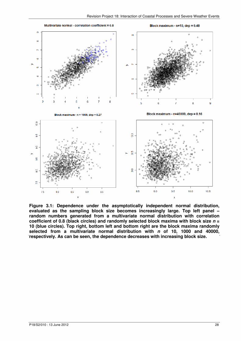
Revision Project 18: Interaction of Coastal Processes and Severe Weather Events
P18/S2/010 : 13 June 2012 28
.
Figure 3.1: Dependence under the asymptotically independent normal distribution, evaluated as the sampling block size becomes increasingly large. Top left panel –random numbers generated from a multivariate normal distribution with correlation coefficient of 0.8 (black circles) and randomly selected block maxima with block size n = 10 (blue circles). Top right, bottom left and bottom right are the block maxima randomly selected from a multivariate normal distribution with n of 10, 1000 and 40000, respectively. As can be seen, the dependence decreases with increasing block size.
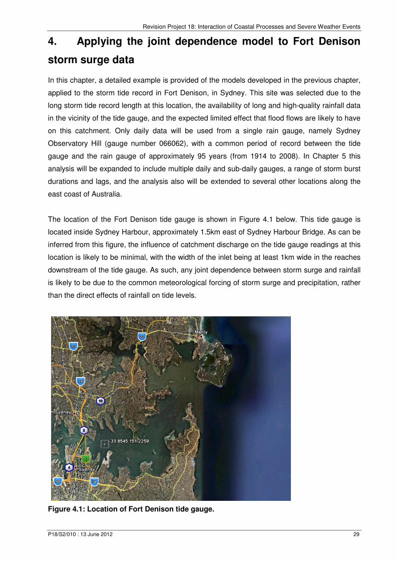
Revision Project 18: Interaction of Coastal Processes and Severe Weather Events
P18/S2/010 : 13 June 2012 29
4. Applying the joint dependence model to Fort Denison
storm surge data
In this chapter, a detailed example is provided of the models developed in the previous chapter,
applied to the storm tide record in Fort Denison, in Sydney. This site was selected due to the
long storm tide record length at this location, the availability of long and high-quality rainfall data
in the vicinity of the tide gauge, and the expected limited effect that flood flows are likely to have
on this catchment. Only daily data will be used from a single rain gauge, namely Sydney
Observatory Hill (gauge number 066062), with a common period of record between the tide
gauge and the rain gauge of approximately 95 years (from 1914 to 2008). In Chapter 5 this
analysis will be expanded to include multiple daily and sub-daily gauges, a range of storm burst
durations and lags, and the analysis also will be extended to several other locations along the
east coast of Australia.
The location of the Fort Denison tide gauge is shown in Figure 4.1 below. This tide gauge is
located inside Sydney Harbour, approximately 1.5km east of Sydney Harbour Bridge. As can be
inferred from this figure, the influence of catchment discharge on the tide gauge readings at this
location is likely to be minimal, with the width of the inlet being at least 1km wide in the reaches
downstream of the tide gauge. As such, any joint dependence between storm surge and rainfall
is likely to be due to the common meteorological forcing of storm surge and precipitation, rather
than the direct effects of rainfall on tide levels.
Figure 4.1: Location of Fort Denison tide gauge.
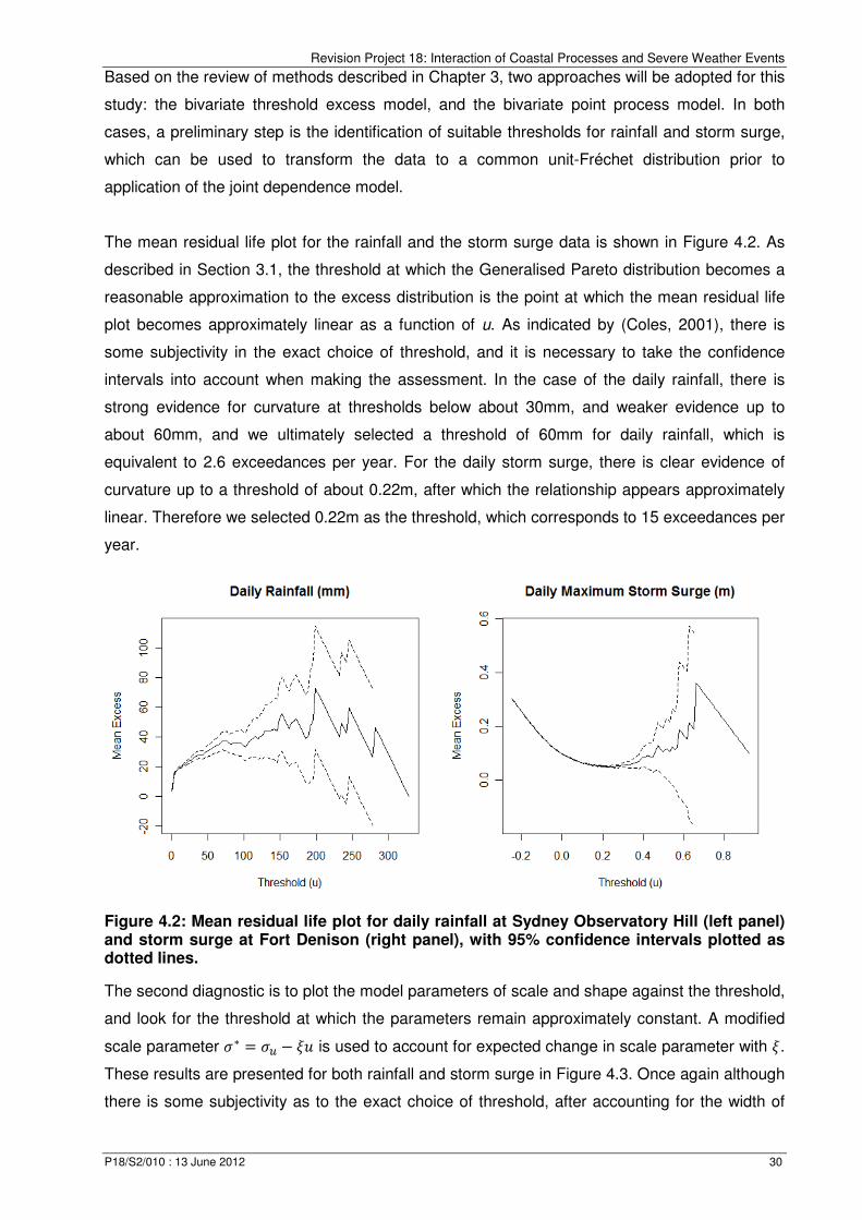
Revision Project 18: Interaction of Coastal Processes and Severe Weather Events
P18/S2/010 : 13 June 2012 30
Based on the review of methods described in Chapter 3, two approaches will be adopted for this
study: the bivariate threshold excess model, and the bivariate point process model. In both
cases, a preliminary step is the identification of suitable thresholds for rainfall and storm surge,
which can be used to transform the data to a common unit-Fréchet distribution prior to
application of the joint dependence model.
The mean residual life plot for the rainfall and the storm surge data is shown in Figure 4.2. As
described in Section 3.1, the threshold at which the Generalised Pareto distribution becomes a
reasonable approximation to the excess distribution is the point at which the mean residual life
plot becomes approximately linear as a function of u. As indicated by (Coles, 2001), there is
some subjectivity in the exact choice of threshold, and it is necessary to take the confidence
intervals into account when making the assessment. In the case of the daily rainfall, there is
strong evidence for curvature at thresholds below about 30mm, and weaker evidence up to
about 60mm, and we ultimately selected a threshold of 60mm for daily rainfall, which is
equivalent to 2.6 exceedances per year. For the daily storm surge, there is clear evidence of
curvature up to a threshold of about 0.22m, after which the relationship appears approximately
linear. Therefore we selected 0.22m as the threshold, which corresponds to 15 exceedances per
year.
Figure 4.2: Mean residual life plot for daily rainfall at Sydney Observatory Hill (left panel) and storm surge at Fort Denison (right panel), with 95% confidence intervals plotted as dotted lines.
The second diagnostic is to plot the model parameters of scale and shape against the threshold,
and look for the threshold at which the parameters remain approximately constant. A modified
scale parameter �∗ = �) − �' is used to account for expected change in scale parameter with �. These results are presented for both rainfall and storm surge in Figure 4.3. Once again although
there is some subjectivity as to the exact choice of threshold, after accounting for the width of
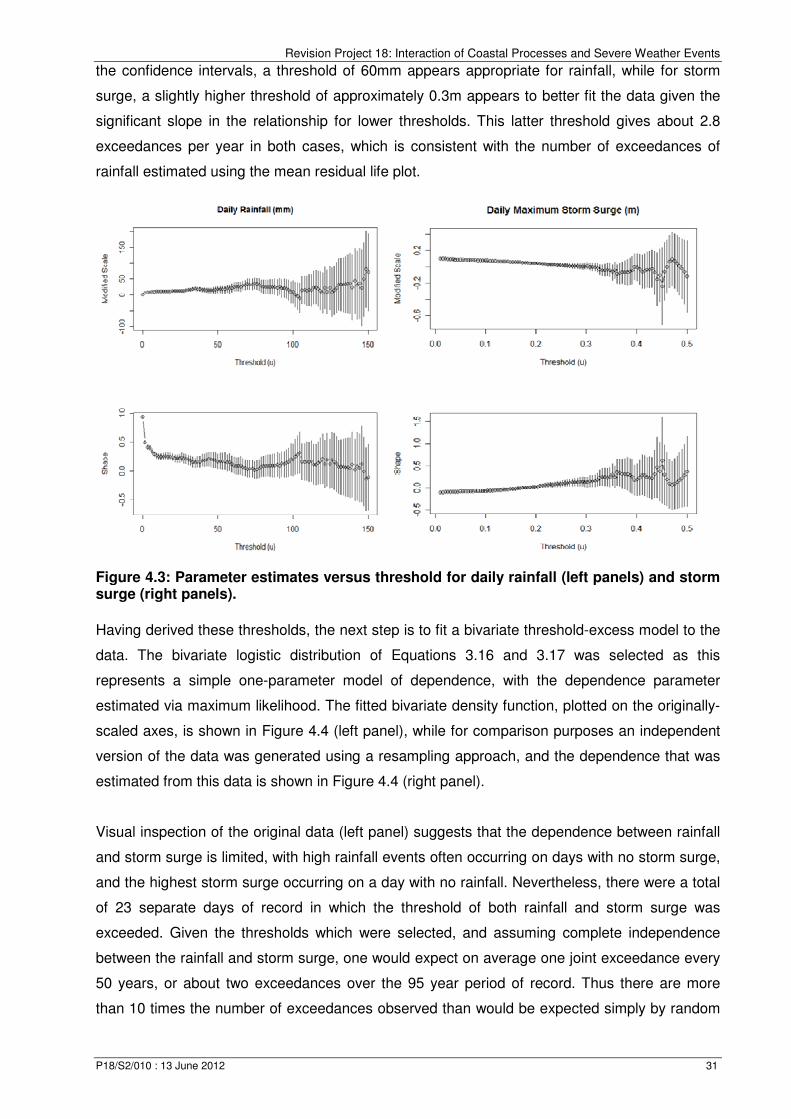
Revision Project 18: Interaction of Coastal Processes and Severe Weather Events
P18/S2/010 : 13 June 2012 31
the confidence intervals, a threshold of 60mm appears appropriate for rainfall, while for storm
surge, a slightly higher threshold of approximately 0.3m appears to better fit the data given the
significant slope in the relationship for lower thresholds. This latter threshold gives about 2.8
exceedances per year in both cases, which is consistent with the number of exceedances of
rainfall estimated using the mean residual life plot.
Having derived these thresholds, the next step is to fit a bivariate threshold-excess model to the
data. The bivariate logistic distribution of Equations 3.16 and 3.17 was selected as this
represents a simple one-parameter model of dependence, with the dependence parameter
estimated via maximum likelihood. The fitted bivariate density function, plotted on the originally-
scaled axes, is shown in Figure 4.4 (left panel), while for comparison purposes an independent
version of the data was generated using a resampling approach, and the dependence that was
estimated from this data is shown in Figure 4.4 (right panel).
Visual inspection of the original data (left panel) suggests that the dependence between rainfall
and storm surge is limited, with high rainfall events often occurring on days with no storm surge,
and the highest storm surge occurring on a day with no rainfall. Nevertheless, there were a total
of 23 separate days of record in which the threshold of both rainfall and storm surge was
exceeded. Given the thresholds which were selected, and assuming complete independence
between the rainfall and storm surge, one would expect on average one joint exceedance every
50 years, or about two exceedances over the 95 year period of record. Thus there are more
than 10 times the number of exceedances observed than would be expected simply by random
Figure 4.3: Parameter estimates versus threshold for daily rainfall (left panels) and storm surge (right panels).
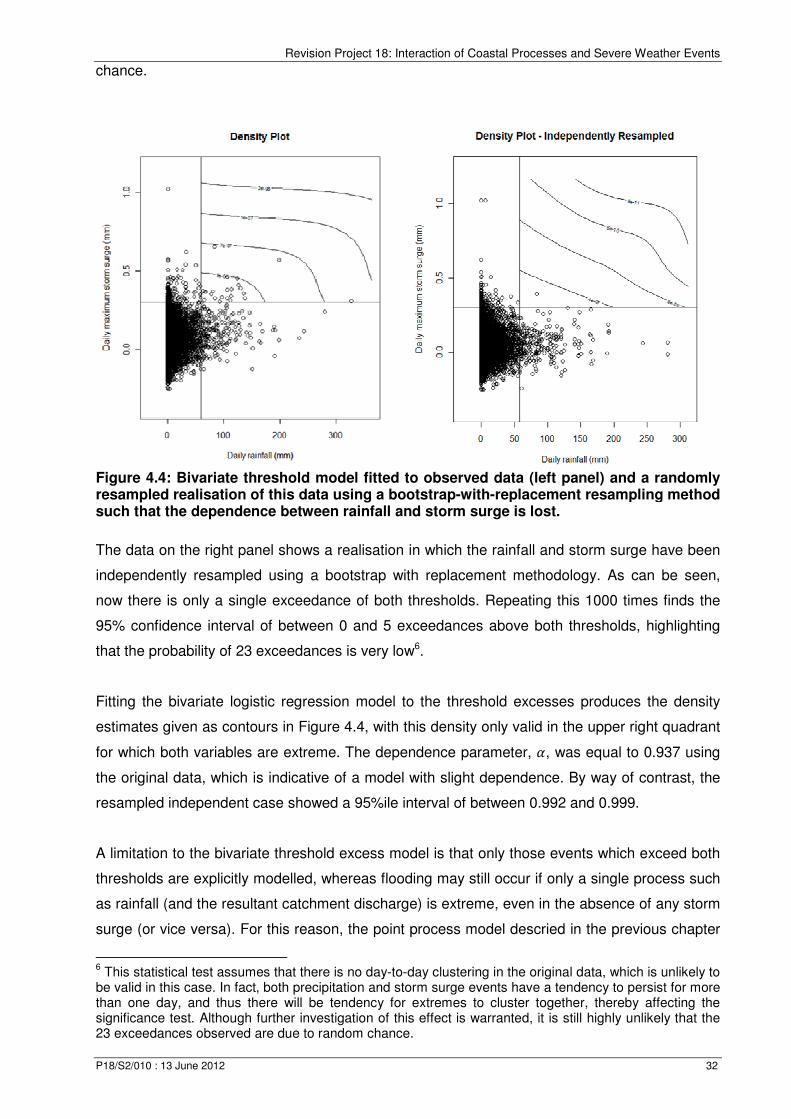
Revision Project 18: Interaction of Coastal Processes and Severe Weather Events
P18/S2/010 : 13 June 2012 32
chance.
The data on the right panel shows a realisation in which the rainfall and storm surge have been
independently resampled using a bootstrap with replacement methodology. As can be seen,
now there is only a single exceedance of both thresholds. Repeating this 1000 times finds the
95% confidence interval of between 0 and 5 exceedances above both thresholds, highlighting
that the probability of 23 exceedances is very low6.
Fitting the bivariate logistic regression model to the threshold excesses produces the density
estimates given as contours in Figure 4.4, with this density only valid in the upper right quadrant
for which both variables are extreme. The dependence parameter, Z, was equal to 0.937 using
the original data, which is indicative of a model with slight dependence. By way of contrast, the
resampled independent case showed a 95%ile interval of between 0.992 and 0.999.
A limitation to the bivariate threshold excess model is that only those events which exceed both
thresholds are explicitly modelled, whereas flooding may still occur if only a single process such
as rainfall (and the resultant catchment discharge) is extreme, even in the absence of any storm
surge (or vice versa). For this reason, the point process model descried in the previous chapter
6 This statistical test assumes that there is no day-to-day clustering in the original data, which is unlikely to
be valid in this case. In fact, both precipitation and storm surge events have a tendency to persist for more than one day, and thus there will be tendency for extremes to cluster together, thereby affecting the significance test. Although further investigation of this effect is warranted, it is still highly unlikely that the 23 exceedances observed are due to random chance.
Figure 4.4: Bivariate threshold model fitted to observed data (left panel) and a randomly resampled realisation of this data using a bootstrap-with-replacement resampling method such that the dependence between rainfall and storm surge is lost.
Revision Project 18: Interaction of Coastal Processes and Severe Weather Events
P18/S2/010 : 13 June 2012 33
is now considered.
The starting point to implementing the point process model is to transform the full record to a
unit-Fréchet distribution, using a combination of a Generalised Pareto distribution for values in
excess of a given threshold, and the empirical distribution function for the remainder of the
values, as described in Equation 3.20. The data are then converted to angular (w) and radial (r)
components as described in Equations 3.22 and 3.23.
To determine the minimum radial distance rmin for which the non-homogenous Poisson process
with limiting intensity function in Equation 3.24 is valid, the histograms of {wi: ri > r0} are
calculated for a range of different values of r0, and the value of r0 was selected at the point
where the shape of the histogram no longer changed significantly. The histograms for different
values of r0 are presented in Figure 4.5. Although some subjectivity exists with regard to the
selection of rmin, a value of = n-1exp(5) was ultimately selected, yielding a total of 446 samples
which exceeded the threshold. The value of the marginal thresholds which corresponded to this
value of rmin, were 62mm and 0.31m, and thus based on the analysis in the context of the
bivariate threshold excess model described earlier, the marginal distributions above this value of
rmin approximately follow a GPD distribution.
Having determined the value of rmin, the next step is to estimate the parameter(s) of the measure
function h(w). Commencing with the logistic model described in equation 3.17, the parameter Z
can be estimated by maximising the log likelihood:
m�Z� = log�Z�� − 1� + �−1 − Z��� logVQ�1 − Q�X + �Z − 2�log�Q��/W + �1 − Q���/W�
for all w with r > rmin. A value of Z of 0.814 was found, and the fitted h(w) was plotted against the
empirical histogram corresponding to this value of rmin and presented as Figure 4.6 (left panel),
with this measure function providing a reasonable fit to the data.
To estimate the significance of this value of Z, the same resampling approach was used as
described previously, such that the properties of the marginal distributions of rainfall and storm
surge are preserved but the joint dependence is eliminated. After repeating this 100 times, the
95% confidence intervals of Z were found to be between 0.861 and 0.867. The observed value
of Z of 0.814 therefore is indicative of mild dependence between storm surge at Fort Dension
and rainfall at Sydney Observatory Hill, consistent with the conclusions of the threshold excess
model described above.
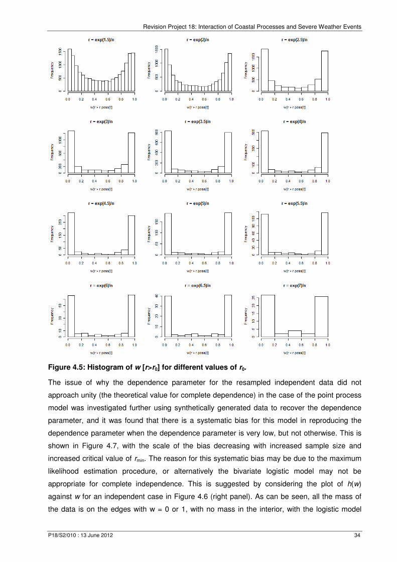
Revision Project 18: Interaction of Coastal Processes and Severe Weather Events
P18/S2/010 : 13 June 2012 34
Figure 4.5: Histogram of w [r>r0] for different values of r0.
The issue of why the dependence parameter for the resampled independent data did not
approach unity (the theoretical value for complete dependence) in the case of the point process
model was investigated further using synthetically generated data to recover the dependence
parameter, and it was found that there is a systematic bias for this model in reproducing the
dependence parameter when the dependence parameter is very low, but not otherwise. This is
shown in Figure 4.7, with the scale of the bias decreasing with increased sample size and
increased critical value of rmin. The reason for this systematic bias may be due to the maximum
likelihood estimation procedure, or alternatively the bivariate logistic model may not be
appropriate for complete independence. This is suggested by considering the plot of h(w)
against w for an independent case in Figure 4.6 (right panel). As can be seen, all the mass of
the data is on the edges with w = 0 or 1, with no mass in the interior, with the logistic model
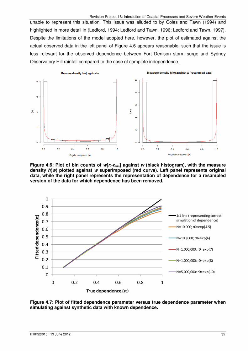
Revision Project 18: Interaction of Coastal Processes and Severe Weather Events
P18/S2/010 : 13 June 2012 35
unable to represent this situation. This issue was alluded to by Coles and Tawn (1994) and
highlighted in more detail in (Ledford, 1994; Ledford and Tawn, 1996; Ledford and Tawn, 1997).
Despite the limitations of the model adopted here, however, the plot of estimated against the
actual observed data in the left panel of Figure 4.6 appears reasonable, such that the issue is
less relevant for the observed dependence between Fort Denison storm surge and Sydney
Observatory Hill rainfall compared to the case of complete independence.
Figure 4.6: Plot of bin counts of w[r>rmin] against w (black histogram), with the measure density h(w) plotted against w superimposed (red curve). Left panel represents original data, while the right panel represents the representation of dependence for a resampled version of the data for which dependence has been removed.
Figure 4.7: Plot of fitted dependence parameter versus true dependence parameter when simulating against synthetic data with known dependence.
0
0.1
0.2
0.3
0.4
0.5
0.6
0.7
0.8
0.9
1
0 0.2 0.4 0.6 0.8 1
Fit
ted
de
pe
nd
en
ce(α
)
True dependence (α)
1:1 line (representing correct
simulation of dependence)
N=10,000; r0=exp(4.5)
N=100,000; r0=exp(6)
N=1,000,000; r0=exp(7)
N=1,000,000; r0=exp(8)
N=5,000,000; r0=exp(10)
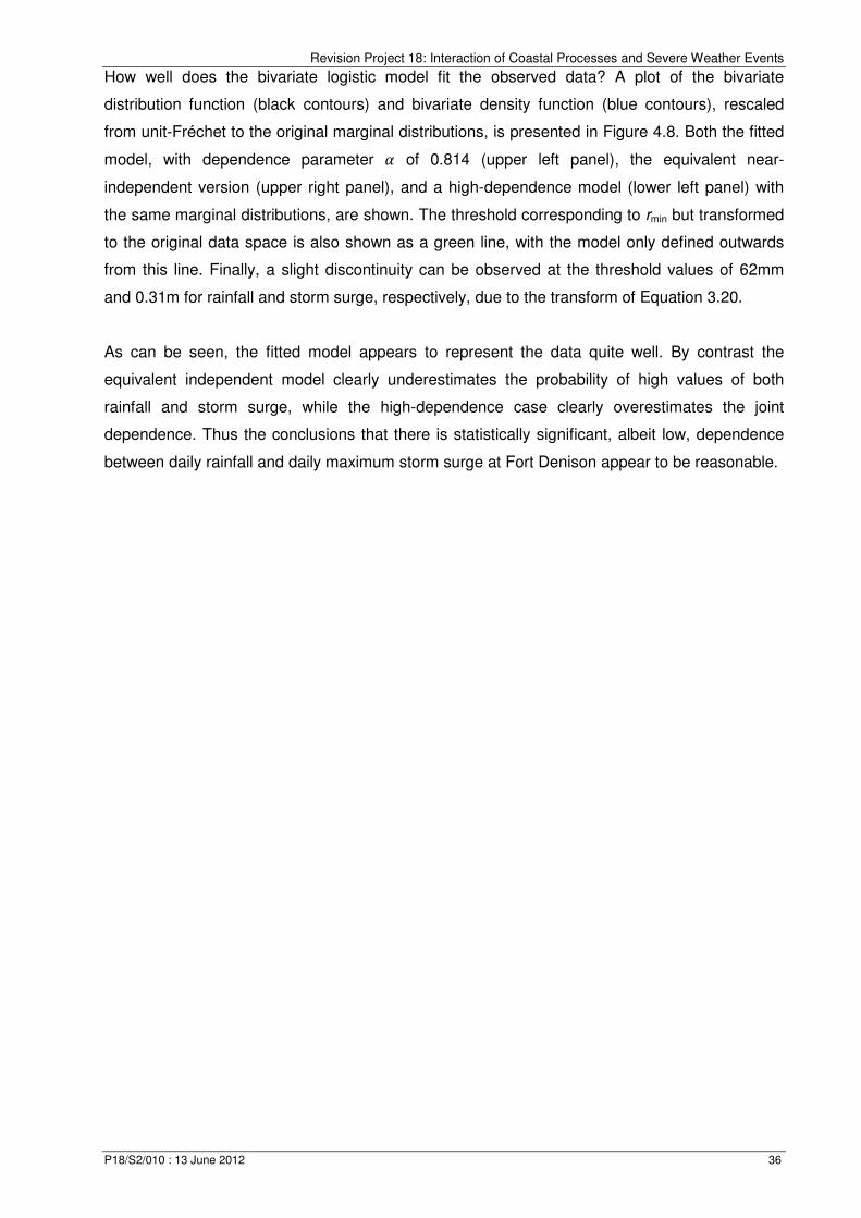
Revision Project 18: Interaction of Coastal Processes and Severe Weather Events
P18/S2/010 : 13 June 2012 36
How well does the bivariate logistic model fit the observed data? A plot of the bivariate
distribution function (black contours) and bivariate density function (blue contours), rescaled
from unit-Fréchet to the original marginal distributions, is presented in Figure 4.8. Both the fitted
model, with dependence parameter Z of 0.814 (upper left panel), the equivalent near-
independent version (upper right panel), and a high-dependence model (lower left panel) with
the same marginal distributions, are shown. The threshold corresponding to rmin but transformed
to the original data space is also shown as a green line, with the model only defined outwards
from this line. Finally, a slight discontinuity can be observed at the threshold values of 62mm
and 0.31m for rainfall and storm surge, respectively, due to the transform of Equation 3.20.
As can be seen, the fitted model appears to represent the data quite well. By contrast the
equivalent independent model clearly underestimates the probability of high values of both
rainfall and storm surge, while the high-dependence case clearly overestimates the joint
dependence. Thus the conclusions that there is statistically significant, albeit low, dependence
between daily rainfall and daily maximum storm surge at Fort Denison appear to be reasonable.

Revision Project 18: Interaction of Coastal Processes and Severe Weather Events
P18/S2/010 : 13 June 2012 37
In the following chapter, both the threshold-excess and point process models will be applied to a
larger dataset, including two other locations (Brisbane and Mackay). Furthermore, a larger set of
daily rainfall records, together with several pluviograph records, will be used to better explore
the importance of distance between tide gauge and rainfall gauge, the duration of the storm
event, and the lag between rainfall event and storm surge event, in determining the magnitude
of dependence between these two physical processes.
Figure 4.8: Joint distribution function (black contours) and density function (blue contours) plotted in the original data space. The upper left panel represents joint distribution with dependence parameter of 0.814, which is based on the maximum likelihood fit to the data. The upper right panel represents the near-independent case (dependence parameter 0.999), while the lower left panel represents a high-dependence case (dependence parameter 0.100). In all cases the marginal distribution of rainfall and storm surge are identical. The green line defines rmin, and thus the bivariate point process model is only defined to the exterior of this line.
Revision Project 18: Interaction of Coastal Processes and Severe Weather Events
P18/S2/010 : 13 June 2012 38
5. Modelling dependence at selected locations
The theoretical approach for modelling bivariate dependence was discussed in detail in Chapter
3, and a worked example of two approaches using Fort Denison storm tide data and Sydney
Observatory Hill daily rainfall data was provided in Chapter 4. In this chapter, the two modelling
approaches that were identified, namely the bivariate threshold-excess model and the point
process model, will be applied to three locations along the east coast of Australia. The focus of
this research will be to determine the influence of a range of factors on the strength of
dependence between rainfall and storm surge, with these factors being the distance between
tide gauge and rainfall gauge, the lag between rainfall and storm surge event, and the influence
of storm burst duration.
The first location considered in this analysis is Fort Denison in Sydney, which was already
shown in Figure 4.1. This gauge was selected due to the length of record at this location, and
because a calibrated hydrodynamic model of the Hawkesbury-Nepean catchment located
approximately 30km north of the tide gauge was available to form the basis for case study (see
Chapter 6).
The second location was a tide gauge in Brisbane, with records extending from 1957 to 2009,
with the location of the tide gauge shown in Figure 5.1 below. This site is largely protected from
the open ocean by the presence of Moreton Island and North Stradbroke Island approximately
25km to the east. Given that the gauge is located at the mouth of the Brisbane River, it is
possible that the water level might be affected by freshwater flows coming from upstream, which
may result in an artificial increase in the level of joint dependence found by statistical modelling
of the rainfall and storm surge. This issue may also be present in several other locations along
the Australian coastline, including Cairns and possibly Townsville which are two other long
storm tide records along the Queensland coastline, and thus needs to be considered as a
possible issue in any joint probability analysis.
The third and final location was Mackay, with storm tide records from 1960 to 2009. This station
is shown in Figure 5.2 below, and is also protected from the open ocean by the presence of the
Great Barrier Reef to the east. This station is located at the end of a pier well away from the
river mouth, and is therefore not likely to be affected by freshwater flows coming from upstream.
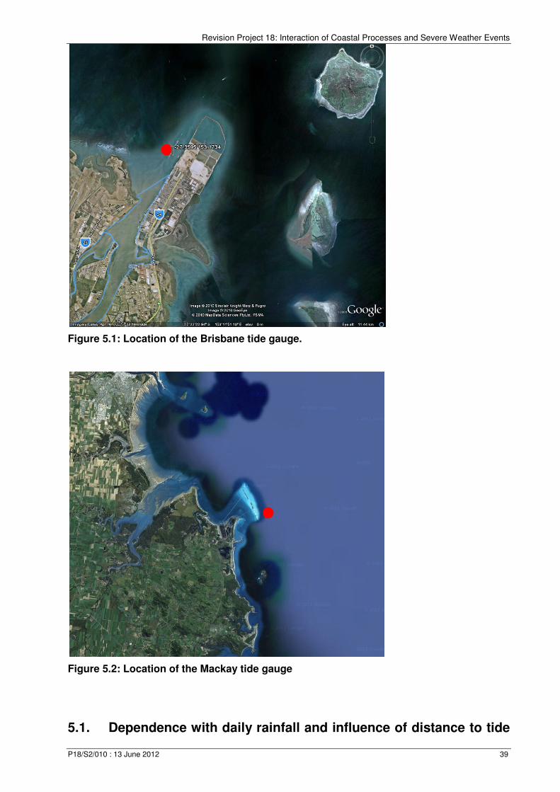
Revision Project 18: Interaction of Coastal Processes and Severe Weather Events
P18/S2/010 : 13 June 2012 39
Figure 5.1: Location of the Brisbane tide gauge.
Figure 5.2: Location of the Mackay tide gauge
5.1. Dependence with daily rainfall and influence of distance to tide
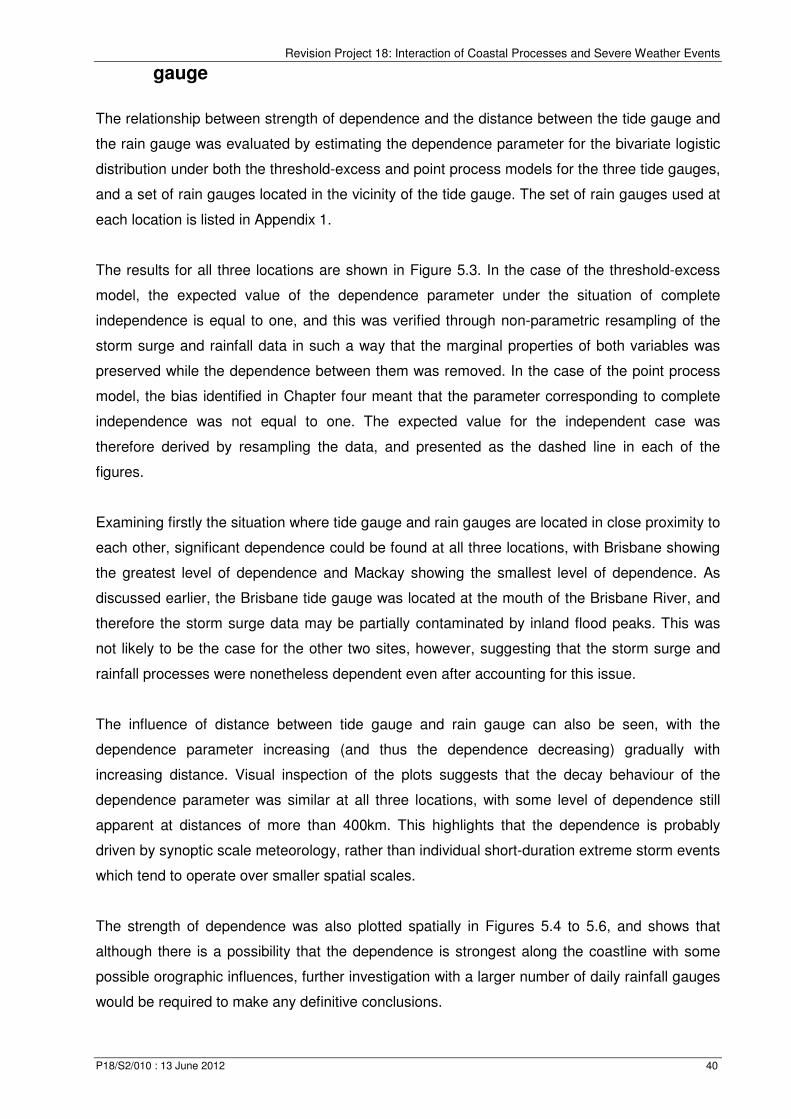
Revision Project 18: Interaction of Coastal Processes and Severe Weather Events
P18/S2/010 : 13 June 2012 40
gauge
The relationship between strength of dependence and the distance between the tide gauge and
the rain gauge was evaluated by estimating the dependence parameter for the bivariate logistic
distribution under both the threshold-excess and point process models for the three tide gauges,
and a set of rain gauges located in the vicinity of the tide gauge. The set of rain gauges used at
each location is listed in Appendix 1.
The results for all three locations are shown in Figure 5.3. In the case of the threshold-excess
model, the expected value of the dependence parameter under the situation of complete
independence is equal to one, and this was verified through non-parametric resampling of the
storm surge and rainfall data in such a way that the marginal properties of both variables was
preserved while the dependence between them was removed. In the case of the point process
model, the bias identified in Chapter four meant that the parameter corresponding to complete
independence was not equal to one. The expected value for the independent case was
therefore derived by resampling the data, and presented as the dashed line in each of the
figures.
Examining firstly the situation where tide gauge and rain gauges are located in close proximity to
each other, significant dependence could be found at all three locations, with Brisbane showing
the greatest level of dependence and Mackay showing the smallest level of dependence. As
discussed earlier, the Brisbane tide gauge was located at the mouth of the Brisbane River, and
therefore the storm surge data may be partially contaminated by inland flood peaks. This was
not likely to be the case for the other two sites, however, suggesting that the storm surge and
rainfall processes were nonetheless dependent even after accounting for this issue.
The influence of distance between tide gauge and rain gauge can also be seen, with the
dependence parameter increasing (and thus the dependence decreasing) gradually with
increasing distance. Visual inspection of the plots suggests that the decay behaviour of the
dependence parameter was similar at all three locations, with some level of dependence still
apparent at distances of more than 400km. This highlights that the dependence is probably
driven by synoptic scale meteorology, rather than individual short-duration extreme storm events
which tend to operate over smaller spatial scales.
The strength of dependence was also plotted spatially in Figures 5.4 to 5.6, and shows that
although there is a possibility that the dependence is strongest along the coastline with some
possible orographic influences, further investigation with a larger number of daily rainfall gauges
would be required to make any definitive conclusions.
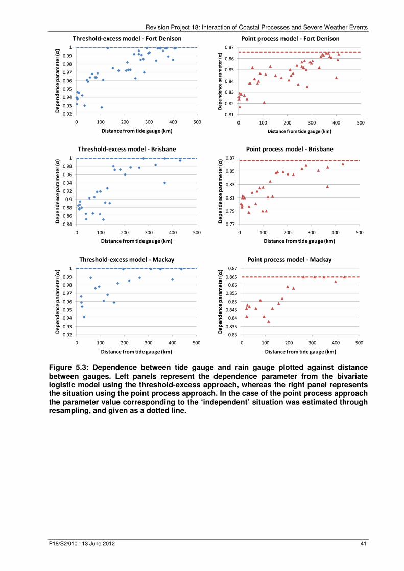
Revision Project 18: Interaction of Coastal Processes and Severe Weather Events
P18/S2/010 : 13 June 2012 41
Figure 5.3: Dependence between tide gauge and rain gauge plotted against distance between gauges. Left panels represent the dependence parameter from the bivariate logistic model using the threshold-excess approach, whereas the right panel represents the situation using the point process approach. In the case of the point process approach the parameter value corresponding to the ‘independent’ situation was estimated through resampling, and given as a dotted line.
0.92
0.93
0.94
0.95
0.96
0.97
0.98
0.99
1
0 100 200 300 400 500
De
pe
nd
en
ce p
ara
me
ter
(α)
Distance from tide gauge (km)
Threshold-excess model - Fort Denison
0.81
0.82
0.83
0.84
0.85
0.86
0.87
0 100 200 300 400 500
De
pe
nd
en
ce p
ara
me
ter
(α)
Distance from tide gauge (km)
Point process model - Fort Denison
0.84
0.86
0.88
0.9
0.92
0.94
0.96
0.98
1
0 100 200 300 400 500
De
pe
nd
en
ce p
ara
me
ter
(α)
Distance from tide gauge (km)
Threshold-excess model - Brisbane
0.77
0.79
0.81
0.83
0.85
0.87
0 100 200 300 400 500
De
pe
nd
en
ce p
ara
me
ter
(α)
Distance from tide gauge (km)
Point process model - Brisbane
0.92
0.93
0.94
0.95
0.96
0.97
0.98
0.99
1
0 100 200 300 400 500
De
pe
nd
en
ce p
ara
me
ter
(α)
Distance from tide gauge (km)
Threshold-excess model - Mackay
0.83
0.835
0.84
0.845
0.85
0.855
0.86
0.865
0.87
0 100 200 300 400 500
De
pe
nd
en
ce p
ara
me
ter
(α)
Distance from tide gauge (km)
Point process model - Mackay

Revision Project 18: Interaction of Coastal Processes and Severe Weather Events
P18/S2/010 : 13 June 2012 42
Figure 5.4: Dependence between daily maximum storm surge at Sydney tide gauge, and daily rainfall in the surrounding region. The tide gauge is represented as a yellow dot; large red dots represent dependence parameter < 0.83; small red dots represent dependence parameter between 0.85 and 0.83, and small blue dots represent dependence parameter > 0.85.

Revision Project 18: Interaction of Coastal Processes and Severe Weather Events
P18/S2/010 : 13 June 2012 43
Figure 5.5: Dependence between daily maximum storm surge at Brisbane tide gauge, and daily rainfall in the surrounding region. The tide gauge is represented as a yellow dot; large red dots represent dependence parameter < 0.83; small red dots represent dependence parameter between 0.85 and 0.83, and small blue dots represent dependence parameter > 0.85.
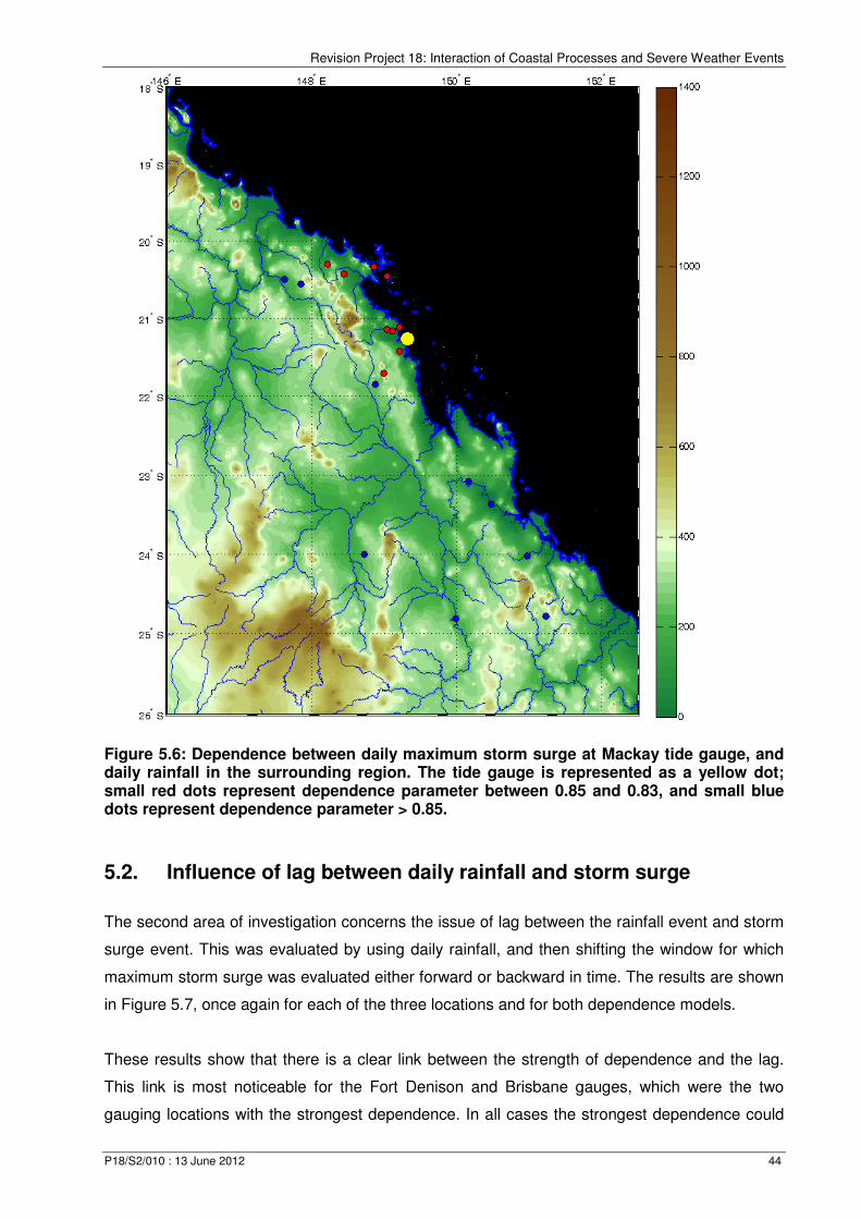
Revision Project 18: Interaction of Coastal Processes and Severe Weather Events
P18/S2/010 : 13 June 2012 44
Figure 5.6: Dependence between daily maximum storm surge at Mackay tide gauge, and daily rainfall in the surrounding region. The tide gauge is represented as a yellow dot; small red dots represent dependence parameter between 0.85 and 0.83, and small blue dots represent dependence parameter > 0.85.
5.2. Influence of lag between daily rainfall and storm surge
The second area of investigation concerns the issue of lag between the rainfall event and storm
surge event. This was evaluated by using daily rainfall, and then shifting the window for which
maximum storm surge was evaluated either forward or backward in time. The results are shown
in Figure 5.7, once again for each of the three locations and for both dependence models.
These results show that there is a clear link between the strength of dependence and the lag.
This link is most noticeable for the Fort Denison and Brisbane gauges, which were the two
gauging locations with the strongest dependence. In all cases the strongest dependence could
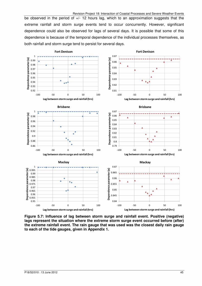
Revision Project 18: Interaction of Coastal Processes and Severe Weather Events
P18/S2/010 : 13 June 2012 45
be observed in the period of +/- 12 hours lag, which to an approximation suggests that the
extreme rainfall and storm surge events tend to occur concurrently. However, significant
dependence could also be observed for lags of several days. It is possible that some of this
dependence is because of the temporal dependence of the individual processes themselves, as
both rainfall and storm surge tend to persist for several days.
Figure 5.7: Influence of lag between storm surge and rainfall event. Positive (negative) lags represent the situation where the extreme storm surge event occurred before (after) the extreme rainfall event. The rain gauge that was used was the closest daily rain gauge to each of the tide gauges, given in Appendix 1.
0.92
0.93
0.94
0.95
0.96
0.97
0.98
0.99
1
-100 -50 0 50 100
De
pe
nd
en
ce p
ara
me
ter
(α)
Lag between storm surge and rainfall (hrs)
Fort Denison
0.81
0.82
0.83
0.84
0.85
0.86
0.87
-100 -50 0 50 100
De
pe
nd
en
ce p
ara
me
ter
(α)
Lag between storm surge and rainfall (hrs)
Fort Denison
0.86
0.88
0.9
0.92
0.94
0.96
0.98
1
-100 -50 0 50 100
De
pe
nd
en
ce p
ara
me
ter
(α)
Lag between storm surge and rainfall (hrs)
Brisbane
0.79
0.8
0.81
0.82
0.83
0.84
0.85
0.86
0.87
-100 -50 0 50 100
De
pe
nd
en
ce p
ara
me
ter
(α)
Lag between storm surge and rainfall (hrs)
Brisbane
0.95
0.955
0.96
0.965
0.97
0.975
0.98
0.985
0.99
0.995
1
-100 -50 0 50 100
De
pe
nd
en
ce p
ara
me
ter
(α)
Lag between storm surge and rainfall (hrs)
Mackay
0.84
0.845
0.85
0.855
0.86
0.865
0.87
-100 -50 0 50 100
De
pe
nd
en
ce p
ara
me
ter
(α)
Lag between storm surge and rainfall (hrs)
Mackay

Revision Project 18: Interaction of Coastal Processes and Severe Weather Events
P18/S2/010 : 13 June 2012 46
5.3. Influence of storm burst duration
The final factor considered is the duration of the storm burst. In the previous sections, the rainfall
data was obtained from a set of daily rain gauges which record accumulated total rainfall up to
9am each morning. Here, pluviograph data is used, for which rainfall data is available in
increments of 6 minutes, with the specific pluviograph stations used in the analysis listed in
Appendix 1. The storm burst duration was then calculated for durations from 6 minutes through
to 72 hours, and the dependence between daily maximum storm surge and storms at all
durations is evaluated.
The results are given in Figure 5.8 and show that there is a sharp increase in dependence from
the shortest duration of 6 minutes up to approximately an hourly duration. After this the strength
of dependence increases only gradually, up to durations of approximately one day. For longer
durations the dependence stays approximately constant. Interestingly, the same pattern is
apparent for all locations, and for all the pluviograph stations that were examined.
The implications for flood estimation practice are significant: for small catchments, including
many urban storm water catchments with rapid response times, the dependence between
rainfall and storm surge is likely to be relatively low, whereas for larger catchments the
dependence becomes much more significant. Such a link between dependence and catchment
response times suggest that the dependence between catchment flows and storm surge will be
heavily influenced by catchment characteristics.
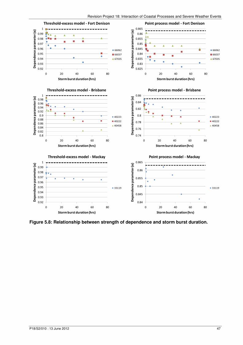
Revision Project 18: Interaction of Coastal Processes and Severe Weather Events
P18/S2/010 : 13 June 2012 47
Figure 5.8: Relationship between strength of dependence and storm burst duration.
0.92
0.93
0.94
0.95
0.96
0.97
0.98
0.99
1
0 20 40 60 80
De
pe
nd
en
ce p
ara
me
ter
(α)
Storm burst duration (hrs)
Threshold-excess model - Fort Denison
66062
66037
67035
0.825
0.83
0.835
0.84
0.845
0.85
0.855
0.86
0.865
0 20 40 60 80
De
pe
nd
en
ce p
ara
me
ter
(α)
Storm burst duration (hrs)
Point process model - Fort Denison
66062
66037
67035
0.8
0.82
0.84
0.86
0.88
0.9
0.92
0.94
0.96
0.98
1
0 20 40 60 80
De
pe
nd
en
ce p
ara
me
ter
(α)
Storm burst duration (hrs)
Threshold-excess model - Brisbane
40223
40222
40458
0.74
0.76
0.78
0.8
0.82
0.84
0.86
0 20 40 60 80
De
pe
nd
en
ce p
ara
me
ter
(α)
Storm burst duration (hrs)
Point process model - Brisbane
40223
40222
40458
0.92
0.93
0.94
0.95
0.96
0.97
0.98
0.99
1
0 20 40 60 80
De
pe
nd
en
ce p
ara
me
ter
(α)
Storm burst duration (hrs)
Threshold-excess model - Mackay
33119
0.84
0.845
0.85
0.855
0.86
0.865
0 20 40 60 80
De
pe
nd
en
ce p
ara
me
ter
(α)
Storm burst duration (hrs)
Point process model - Mackay
33119

Revision Project 18: Interaction of Coastal Processes and Severe Weather Events
P18/S2/010 : 13 June 2012 48
6. Case study: Hawkesbury Nepean model
6.1. Background
In the previous chapters, the emphasis was on the statistical modelling of the joint dependence
between rainfall and storm surge at different locations along the east Australian coastline. This
involved identifying a statistical model (in this case, a bivariate logistic model) and applying this
model to storm tide and rainfall datasets to obtain a dependence parameter which indicates the
extent to which the two variables co-vary. This dependence parameter was found to vary as a
function of various factors, including geographic location, distance between tide gauge and rain
gauge, storm burst duration and lag between rainfall event and storm surge event. Having
identified the appropriate amount of dependence, this chapter addresses the question: how
should this information be used to estimate the design flood level at any given location?
Once again following the methodology of Coles and Tawn (1994), the quantity of interest is the
exceedance probability of a ‘design parameter’ v, when this parameter is influenced by more
than one physically distinct – but potentially dependent – constituent process. In this chapter v is
assumed to be the design flood level at some location of interest, but it could equally refer to a
range of other variables which can be used for engineering design such as flood flow rate or
some other flood parameter. It is further assumed that the primary factors influencing flood
height will be a combination of precipitation-induced flows from the catchment (X), and storm
tide affecting the downstream boundary (Y).
A ‘failure region’, Av, is defined given in terms of these two constituent processes, as follows:
no = {�x, y� ∈ ℝ\: t�x, y� > u�} (6.1)
where b(x,y) is referred to as the ‘boundary function’ which translates the two-dimensional input
data to a one-dimensional variable of interest such as the flood level. Such a function may be a
simple functional such as the examples given in Coles and Tawn (1994), or much more
complex; in the current study, hydrologic and hydrodynamic modelling was performed to
estimate the flood levels which arise from different combinations of rainfall and storm surge/tide,
and thus the functional form of b(x,y) is embedded within these models. The failure region Av
therefore can be interpreted as the set of values of the constituent processes (x,y) which cause
the flood levels to be greater than a specified design flood level v, using the transformation
between constituent processes and flood levels as contained in the functional b(x,y). The
objective of this analysis is to find � = Pr{�%, C� ∈ no}; in other words, the probability that the
rainfall and storm surge is contained within the failure region Av and thus cause floods that are
greater than the design flood value. The inverse problem is also often of interest: namely, finding
Revision Project 18: Interaction of Coastal Processes and Severe Weather Events
P18/S2/010 : 13 June 2012 49
the flood level v which will be exceeded at a given probability p. For example we may wish to
know the value of the flood level which has a 1% Annual Exceedance Probability (AEP).
As with the previous chapters, the failure region no can be described in the unit-Fréchet scale
via:
nvo = ����no� (6.2)
where Ψ�� describes the transformation to unit-Fréchet using equation 3.20. With reference to
the form of bivariate extreme value distribution given in equation 3.10 and the non-homogenous
Poisson process in equation 3.24, one can write the probability of the constituent processes x
and y being within the ‘failure region’ nvo defined at a particular value of v via:
Pr{��7, J7� ∈ no; x = 1,… , �} = 1 − exp{−kVnvoX} (6.3)
where, in the pseudo-polar coordinate system described by transformations in equation 3.22
and 3.23,
kVnvoX = M j�\Ojℎ�Q�OQyz{ (6.4)
The interpretation of equations 6.3 and 6.4 is simple. Having identified a given form of the
measure function h(w) such as the bivariate logistic distribution in Equation 3.17, one needs to
integrate the function over the set of values of x and y (or equivalently, r and w) for which the
flood level is above v, to obtain the exceedance probability associated with that flood level.
Numerical methods can be used for this integration.
6.2. Modelling flood height
The ‘boundary function’ b(x,y) represents the transform from the bivariate input processes of
extreme rainfall and storm surge/tide, and the response variable of interest such as flood level.
In reality there are a number of steps involved in such a hydrologic/hydraulic modelling study,
which can differ considerably based on the availability of historical data and a range of other
factors such as available budget and the personal preferences of the modeller. The terminology
in the previous section was kept sufficiently general to encompass a wide range of possible
modelling approaches.
A case study was developed in which hydrologic and hydraulic models have been applied to
simulate the tidal and inland reaches of the Hawkesbury/Nepean system. This original model
was developed as part of an Environmental Impact Statement in the 1990s as part of
Revision Project 18: Interaction of Coastal Processes and Severe Weather Events
P18/S2/010 : 13 June 2012 50
investigations for works to upgrade the spillway capacity of Warragamba Dam. The study
included a detailed analysis of the existing flooding behaviour and was carried out by Webb
McKeown and Associates (Webb McKeown and Associates, 1996). The outcomes were subject
to rigorous technical reviews by a range of parties including Sydney Water, the then Department
of Land and Water Conservation, the Bureau of Meteorology and other established experts
within relevant fields.
The hydrologic model used was RORB, and the hydraulic model was RUBICON. The RORB
model was calibrated and then evaluated using historical records available for five of the events
between June 1964 and April 1988. The RUBICON hydrodynamic model software was used to
quantify the hydraulic aspects of the flood behaviour (e.g. flood levels and velocities). RUBICON
is a fully dynamic computer-based 1D model and uses different elements to simulate complex
flow over floodplains and through channel systems. The hydraulic model was established to
cover the entire area from Lake Burragorang to the ocean at Broken Bay. Ultimately the process
of calibrating and evaluating the RUBICON model was undertaken using recorded information
for 11 individual historical events. The models were then used to determine design flood
behaviour of the system.
The calibrated RUBICON model of the Hawkesbury/Nepean has been maintained by WMAwater
(previously Webb McKeown and Associates) since this original study and was selected for this
project as there is a very high flood gradient along the river even though the river is tidal for 140
km upstream of the estuary inlet under non-flood conditions. The flood height (stage) as a result
of different combinations of rainfall and storm tide are shown in Figure 6.1 across the full
modelling domain, and in Figure 6.2 for the portion of the domain near the coast which is most
affected by the interaction between catchment discharge and storm surge.
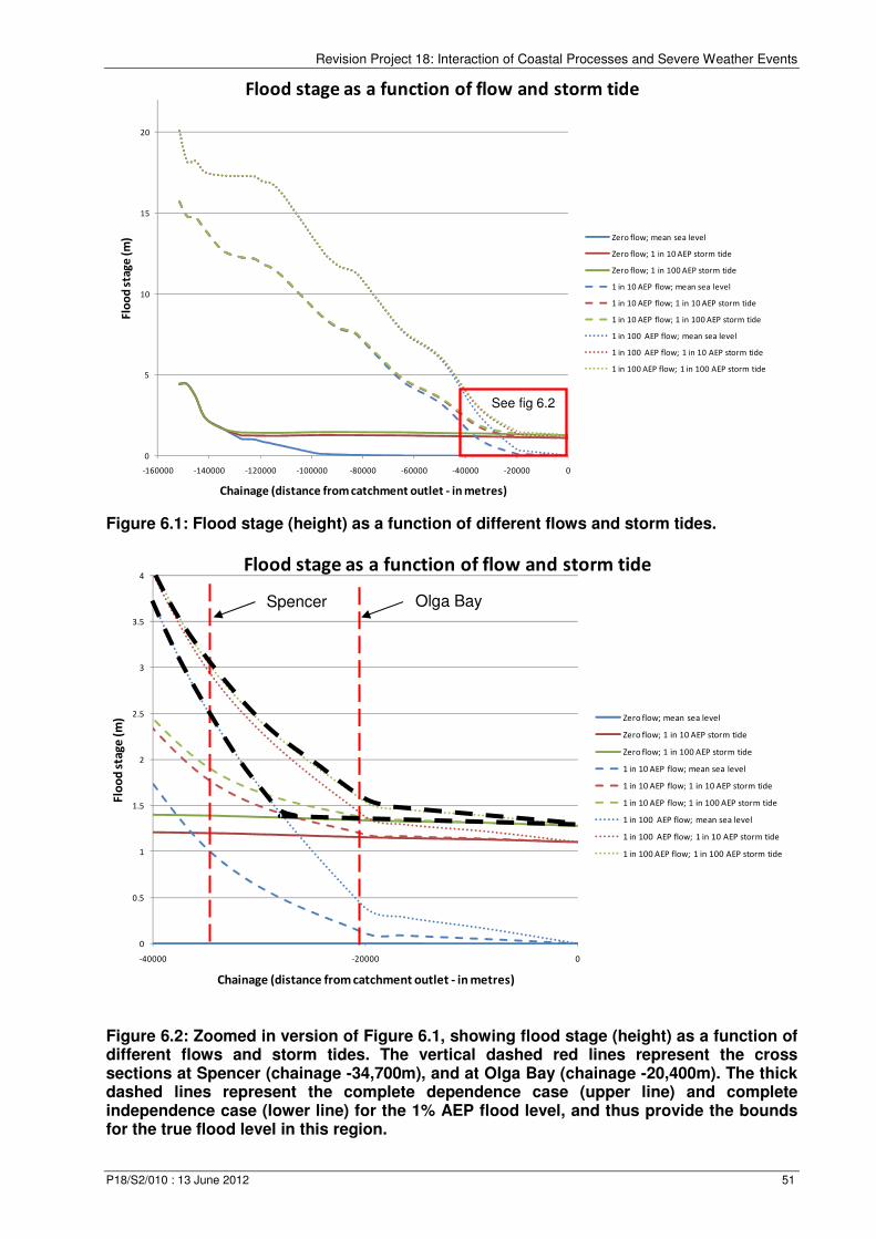
Revision Project 18: Interaction of Coastal Processes and Severe Weather Events
P18/S2/010 : 13 June 2012 51
Figure 6.1: Flood stage (height) as a function of different flows and storm tides.
Figure 6.2: Zoomed in version of Figure 6.1, showing flood stage (height) as a function of different flows and storm tides. The vertical dashed red lines represent the cross sections at Spencer (chainage -34,700m), and at Olga Bay (chainage -20,400m). The thick dashed lines represent the complete dependence case (upper line) and complete independence case (lower line) for the 1% AEP flood level, and thus provide the bounds for the true flood level in this region.
0
5
10
15
20
-160000 -140000 -120000 -100000 -80000 -60000 -40000 -20000 0
Flo
od
sta
ge
(m
)
Chainage (distance from catchment outlet - in metres)
Flood stage as a function of flow and storm tide
Zero flow; mean sea level
Zero flow; 1 in 10 AEP storm tide
Zero flow; 1 in 100 AEP storm tide
1 in 10 AEP flow; mean sea level
1 in 10 AEP flow; 1 in 10 AEP storm tide
1 in 10 AEP flow; 1 in 100 AEP storm tide
1 in 100 AEP flow; mean sea level
1 in 100 AEP flow; 1 in 10 AEP storm tide
1 in 100 AEP flow; 1 in 100 AEP storm tide
0
0.5
1
1.5
2
2.5
3
3.5
4
-40000 -20000 0
Flo
od
sta
ge
(m
)
Chainage (distance from catchment outlet - in metres)
Flood stage as a function of flow and storm tide
Zero flow; mean sea level
Zero flow; 1 in 10 AEP storm tide
Zero flow; 1 in 100 AEP storm tide
1 in 10 AEP flow; mean sea level
1 in 10 AEP flow; 1 in 10 AEP storm tide
1 in 10 AEP flow; 1 in 100 AEP storm tide
1 in 100 AEP flow; mean sea level
1 in 100 AEP flow; 1 in 10 AEP storm tide
1 in 100 AEP flow; 1 in 100 AEP storm tide
Olga Bay Spencer
See fig 6.2
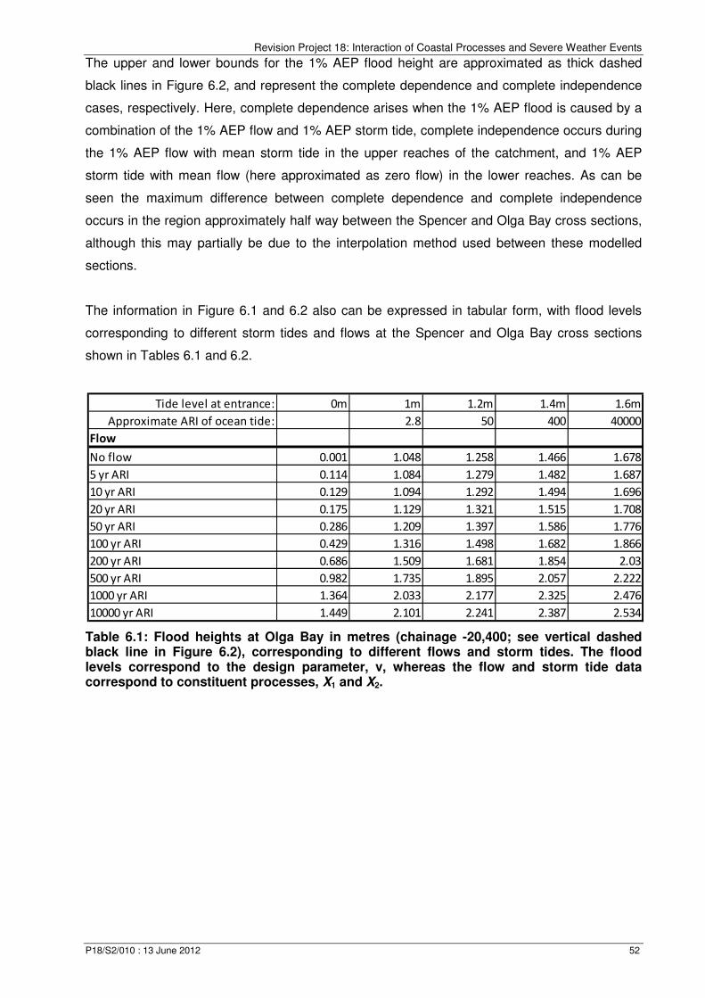
Revision Project 18: Interaction of Coastal Processes and Severe Weather Events
P18/S2/010 : 13 June 2012 52
The upper and lower bounds for the 1% AEP flood height are approximated as thick dashed
black lines in Figure 6.2, and represent the complete dependence and complete independence
cases, respectively. Here, complete dependence arises when the 1% AEP flood is caused by a
combination of the 1% AEP flow and 1% AEP storm tide, complete independence occurs during
the 1% AEP flow with mean storm tide in the upper reaches of the catchment, and 1% AEP
storm tide with mean flow (here approximated as zero flow) in the lower reaches. As can be
seen the maximum difference between complete dependence and complete independence
occurs in the region approximately half way between the Spencer and Olga Bay cross sections,
although this may partially be due to the interpolation method used between these modelled
sections.
The information in Figure 6.1 and 6.2 also can be expressed in tabular form, with flood levels
corresponding to different storm tides and flows at the Spencer and Olga Bay cross sections
shown in Tables 6.1 and 6.2.
Table 6.1: Flood heights at Olga Bay in metres (chainage -20,400; see vertical dashed black line in Figure 6.2), corresponding to different flows and storm tides. The flood levels correspond to the design parameter, v, whereas the flow and storm tide data correspond to constituent processes, X1 and X2.
Tide level at entrance: 0m 1m 1.2m 1.4m 1.6m
Approximate ARI of ocean tide: 2.8 50 400 40000
Flow
No flow 0.001 1.048 1.258 1.466 1.678
5 yr ARI 0.114 1.084 1.279 1.482 1.687
10 yr ARI 0.129 1.094 1.292 1.494 1.696
20 yr ARI 0.175 1.129 1.321 1.515 1.708
50 yr ARI 0.286 1.209 1.397 1.586 1.776
100 yr ARI 0.429 1.316 1.498 1.682 1.866
200 yr ARI 0.686 1.509 1.681 1.854 2.03
500 yr ARI 0.982 1.735 1.895 2.057 2.222
1000 yr ARI 1.364 2.033 2.177 2.325 2.476
10000 yr ARI 1.449 2.101 2.241 2.387 2.534

Revision Project 18: Interaction of Coastal Processes and Severe Weather Events
P18/S2/010 : 13 June 2012 53
Table 6.2: Flood heights at Spencer in metres (chainage -34,700; see vertical dashed black line in Figure 6.2), corresponding to different flows and storm tides. The flood levels correspond to the design parameter, v, whereas the flow and storm tide data correspond to constituent processes, X1 and X2.
Having estimated values of the boundary function b(x,y), producing flood levels for different
combinations of discharge and storm tide at both cross sections, the next step is to superimpose
this data onto the bivariate point process model. The dependence parameter of 0.814 was used
based on the parameter estimate at Fort Denison, although the sensitivity to this parameter also
was also considered.
This superposition is shown in Figure 6.3. Note the dependence contours here are equivalent to
the contours shown in Figure 4.8 (upper left panel), except now the marginal distributions are
presented in terms of their exceedance probabilities. The solid green region represents the
region below the critical threshold rmin, and therefore the point process model is unreliable in this
region.
A graphical interpretation of equations 6.3 and 6.4 is as follows. If the interest is the exceedance
probability of a flood level, say a level of 1.4m in Olga Bay, then one simply needs to integrate
the density function (blue contours) upwards from this line to derive the probability that this level
will be exceeded. This can be repeated for a range of flood levels, and the flood level
corresponding to a desired exceedance probability can be found accordingly. Note, however,
that only those flood levels wholly outside of the green region are defined via this method, and
therefore the method is only able to estimate high flood events. The plot of flood level against
exceedance probability is given in Figure 6.4, and as can be seen the lowest flood levels
correspond approximately to the 1 in 1 year flood event, and thus the limitations imposed by the
threshold do not pose a severe restriction for use of this method for most practical flood
estimation applications. The upper bound was selected somewhat arbitrarily to be the 1% AEP
event, although a more careful review of the extent to which the results can be extrapolated
Tide level at entrance: 0m 1m 1.2m 1.4m 1.6m
Approximate ARI of ocean tide: 2.8 50 400 40000
Flow
No flow 0.002 1.09 1.306 1.519 1.737
5 yr ARI 0.913 1.626 1.782 1.941 2.104
10 yr ARI 1.007 1.694 1.845 2 2.159
20 yr ARI 1.29 1.909 2.049 2.193 2.341
50 yr ARI 1.876 2.374 2.49 2.612 2.737
100 yr ARI 2.497 2.895 2.99 3.089 3.194
200 yr ARI 3.353 3.643 3.714 3.791 3.873
500 yr ARI 4.122 4.345 4.402 4.462 4.526
1000 yr ARI 4.919 5.091 5.134 5.181 5.231
10000 yr ARI 5.083 5.247 5.286 5.334 5.378

Revision Project 18: Interaction of Coastal Processes and Severe Weather Events
P18/S2/010 : 13 June 2012 54
Figure 6.3: Superposition of bivariate point process model fitted to Fort Denison storm surge and Sydney Observatory Hill daily rainfall data (dependence parameter α = 0.814), and the water levels at the Olga Bay (upper panel) and Spencer (lower panel) cross sections in the Hawkesbury-Nepean estuary. The model is only defined above the filled green region, with the distribution and density function given as black and blue contours, respectively. The original rainfall and storm surge data, given in terms of the estimated exceedance probabilities, are shown as black open circles. Finally, contours of water levels at the Olga Bay and Spencer cross sections, based on a linear interpolation of the exceedance probabilities shown in Tables 6.1 and 6.2, are given as red lines.

Revision Project 18: Interaction of Coastal Processes and Severe Weather Events
P18/S2/010 : 13 June 2012 55
Figure 6.4: Water levels at Olga Bay (upper panel) and Spencer (lower panel) cross sections in the Hawkesbury-Nepean model, plotted against exceedance probability, for different levels dependence between rainfall and storm surge. In particular, dependence ranges from near-independence (blue line; dependence parameter α = 0.999) through to high dependence (red line; dependence parameter α = 0.020). The observed dependence between Fort Denison tide gauge storm surge data and Sydney Observatory Hill daily rainfall (black line; dependence parameter α = 0.814) and a lower level of dependence (green line; dependence parameter α = 0.950) are also shown.
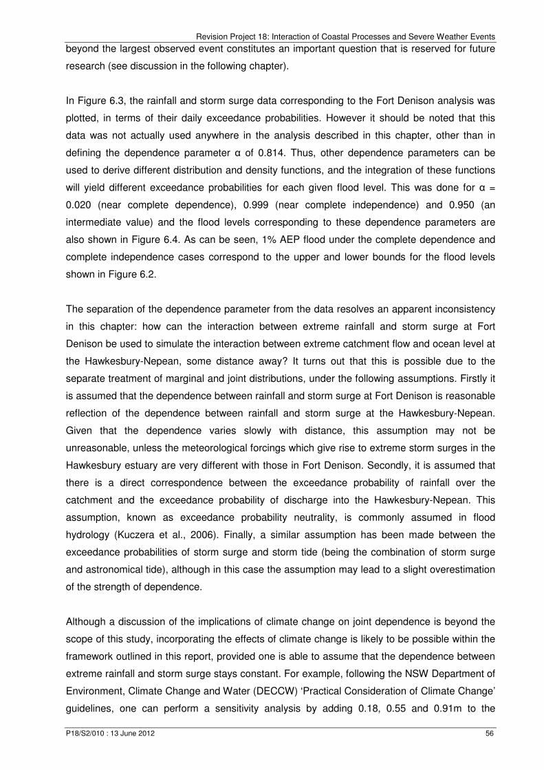
Revision Project 18: Interaction of Coastal Processes and Severe Weather Events
P18/S2/010 : 13 June 2012 56
beyond the largest observed event constitutes an important question that is reserved for future
research (see discussion in the following chapter).
In Figure 6.3, the rainfall and storm surge data corresponding to the Fort Denison analysis was
plotted, in terms of their daily exceedance probabilities. However it should be noted that this
data was not actually used anywhere in the analysis described in this chapter, other than in
defining the dependence parameter α of 0.814. Thus, other dependence parameters can be
used to derive different distribution and density functions, and the integration of these functions
will yield different exceedance probabilities for each given flood level. This was done for α =
0.020 (near complete dependence), 0.999 (near complete independence) and 0.950 (an
intermediate value) and the flood levels corresponding to these dependence parameters are
also shown in Figure 6.4. As can be seen, 1% AEP flood under the complete dependence and
complete independence cases correspond to the upper and lower bounds for the flood levels
shown in Figure 6.2.
The separation of the dependence parameter from the data resolves an apparent inconsistency
in this chapter: how can the interaction between extreme rainfall and storm surge at Fort
Denison be used to simulate the interaction between extreme catchment flow and ocean level at
the Hawkesbury-Nepean, some distance away? It turns out that this is possible due to the
separate treatment of marginal and joint distributions, under the following assumptions. Firstly it
is assumed that the dependence between rainfall and storm surge at Fort Denison is reasonable
reflection of the dependence between rainfall and storm surge at the Hawkesbury-Nepean.
Given that the dependence varies slowly with distance, this assumption may not be
unreasonable, unless the meteorological forcings which give rise to extreme storm surges in the
Hawkesbury estuary are very different with those in Fort Denison. Secondly, it is assumed that
there is a direct correspondence between the exceedance probability of rainfall over the
catchment and the exceedance probability of discharge into the Hawkesbury-Nepean. This
assumption, known as exceedance probability neutrality, is commonly assumed in flood
hydrology (Kuczera et al., 2006). Finally, a similar assumption has been made between the
exceedance probabilities of storm surge and storm tide (being the combination of storm surge
and astronomical tide), although in this case the assumption may lead to a slight overestimation
of the strength of dependence.
Although a discussion of the implications of climate change on joint dependence is beyond the
scope of this study, incorporating the effects of climate change is likely to be possible within the
framework outlined in this report, provided one is able to assume that the dependence between
extreme rainfall and storm surge stays constant. For example, following the NSW Department of
Environment, Climate Change and Water (DECCW) ‘Practical Consideration of Climate Change’
guidelines, one can perform a sensitivity analysis by adding 0.18, 0.55 and 0.91m to the
Revision Project 18: Interaction of Coastal Processes and Severe Weather Events
P18/S2/010 : 13 June 2012 57
extreme sea level at each exceedance probability, and 10%, 20% and 30% to the peak rainfall
at each exceedance probability, and via the hydrologic and hydrodynamic modelling, revise the
boundary function b(x,y) and thus the values in Tables 6.1 and 6.2. Such an analysis will result
in shifted red contours in Figure 6.3 following the new flood levels. However, assuming a
constant dependence parameter, the distribution and density functions in Figure 6.3 will not
change. Therefore, estimating the revised flood heights will use an identical methodology to
what has been described here, but with changed boundary function incorporating the changes in
the marginal distributions of rainfall/discharge and storm surge/tide. The extent to which the
dependence parameter can be assumed to stay constant is uncertain, however, and will require
further work along the lines of (Abbs and McInnes, 2010) to verify.

Revision Project 18: Interaction of Coastal Processes and Severe Weather Events
P18/S2/010 : 13 June 2012 58
7. Conclusions and Recommendations
7.1. Research summary
This report outlines the results of a pilot study into both the presence of joint dependence
between extreme rainfall and storm surge in the coastal zone, as well as the development of a
methodology to translate this information into design flood levels or other design flood quantiles.
The outcomes of this work are as follows:
1) A dataset has been compiled, with assistance from EngTest at Adelaide University,
which can support an empirical study into the joint dependence between rainfall and
storm surge across the Australian coastline. Specifically, the available dataset comprises
storm tide data at 16 locations from 1991-2010 from the Australian Baseline Sea Level
Monitoring Project (ABSLMP), a further 74 tide gauges locations from the National Tidal
Centre, as well as a large quantity of daily and sub-daily rainfall data from the Bureau of
Meteorology. Furthermore, additional data on synoptic systems including historical
records of cyclone tracks is also available, and may be used to support a more detailed
investigation into the conditions under which extreme rainfall and storm surge events are
likely to occur together.
2) A detailed review of the statistical literature was conducted to identify appropriate models
that can be used to estimate design floods when they are caused by more than one
physical process. Given the emphasis on extremes, this review focused on bivariate
extreme value models as the main class of model to simulate the tail ends of a statistical
distribution. Specifically, the bivariate point process extreme value model developed by
Coles and Tawn (1994) was found to be appropriate as it was able to handle the
situation where either only a single physical process or multiple physical processes are
extreme. Code to implement this model was developed as part of this pilot study, using
the R statistical programming language.
3) Two extreme value modelling frameworks – namely a bivariate threshold-excess
approach and a point process approach – were implemented at three locations along the
east Australian coastline: Sydney, Brisbane and Mackay. Statistically significant
dependence was detected at all these locations, with the greatest level of dependence
for Brisbane, and the lowest level for Mackay. It is possible that the strength of
dependence at Brisbane is partially attributable to the location of the tide gauge which is
at the mouth of the Brisbane River, however this is unlikely to be the case for both
Sydney and Mackay. Therefore it is concluded that there is a tendency for extreme
rainfall and extreme storm surges to co-occur, and as such will need to be incorporated

Revision Project 18: Interaction of Coastal Processes and Severe Weather Events
P18/S2/010 : 13 June 2012 59
into flood estimation practice.
4) Using these case study locations, a range of factors which might influence the strength
of dependence between rainfall and storm surge were investigated. Firstly, the spatial
range of dependence was considered, and statistically significant dependence could be
detected over spatial distances of up to several hundred kilometres, although the
strongest dependence could be detected where the tide gauge and the rainfall gauge
were about 30km apart. Secondly, the influence of a lag between rainfall event and
storm tide event was evaluated, and significant dependence could be found for lags of
up to several days between the rainfall event and the surge event. Finally, the
implications of storm burst duration were investigated, and once again a clear
relationship could be found with dependence increasing sharply from the finest 6-minute
timescale to the hourly timescale, and then gradually until a storm burst duration of about
one day, whereupon the dependence stayed approximately constant.
5) A number of possible biases have been identified in the estimation of dependence
parameters between rainfall and storm surge, and in most cases these biases are in the
direction of an overestimation of the strength of dependence. The first of these is that in
locations around Australia, including in Brisbane considered here, the tide gauge is
located at the mouth of a river, and therefore is partially influenced by catchment
flooding. The second relates to the use of storm surge data rather than storm tide data,
with the latter likely to show lower dependence with rainfall. This is because astronomic
tides are unlikely to co-vary with rainfall, and the range of tides is much greater than the
range of the storm surge in most locations where data is available (see Table 2.1). The
final issue relates to the asymptotic assumptions of the dependence model, with a
sensitivity study showing that the bivariate logistic model was biased for very low levels
of dependence. The combination of these biases is likely to result in a slight
overestimation of the ensuing flood levels, and possible approaches to reduce this bias
are identified in Section 7.3 below.
6) Finally, a methodology was described where information on the level of dependence
could be used to estimate flood heights at any given location, and a case study in the
Hawkesbury-Nepean river system was developed to illustrate this methodology. The
methodology involved combining information on the dependence between rainfall and
storm surge/tide with a set of hydrodynamic model runs forced by various combinations
of rainfall and storm tide, to derive flood levels at specified exceedance probabilities.
Importantly, once these model runs have been completed, the flood levels can be
estimated as a smoothly varying function throughout a given estuary, even though
relative influence of the different forcing processes are likely to change from upstream
Revision Project 18: Interaction of Coastal Processes and Severe Weather Events
P18/S2/010 : 13 June 2012 60
(rainfall-dominated) to further downstream (runoff-dominated).
Having conducted this study, how can this information be used to develop guidelines as part of
the Australian Rainfall and Runoff flood estimation guidelines? This is discussed in the following
section.
7.2. Recommended form of guidance into joint dependence of
extreme rainfall and storm surge in the coastal zone
Although there are a number of outstanding research questions, this pilot study was successful
in modelling the dependence between rainfall and storm surge, and translating this information
into a flood level at a specific estuary. Based on these results it is recommended that guidance
on joint dependence in Australian Rainfall and Runoff be provided on four separate issues.
Firstly, guidance is required on the magnitude of dependence between rainfall and storm surge
at all the locations for which sufficient data is available, with a view to providing spatial maps of
how the dependence changes along the Australian coastline. This could be combined with
information on how dependence changes with storm burst duration or lag between rainfall and
storm surge event, such that an estimate of the expected dependence parameter can be found
for any catchment of interest at any location along the Australian coastline.
Secondly, guidance is required on how to translate this information into a design flood level. The
methodology described in Chapter 6 is recommended, in which flood levels are estimated for
different combinations of rainfall/flow and storm surge/tide (in terms of their exceedance
probabilities) using a hydrodynamic model, and this information superimposed onto the
dependence model such as given in Figure 6.3, with the integration to the right of each flood
level contour providing the exceedance probability for that flood level. This could be
implemented as a simple software tool, taking as inputs the dependence parameter (and
possibly the dependence model), and the flood levels corresponding to different exceedance
probabilities of rainfall/runoff and storm tide such as provided in Tables 6.1 and 6.2. The R-code
length for implementing this part of the modelling is less than a single page, and the
computations take less than a minute to complete, highlighting the relatively low complexity of
implementing this in practice. Although further attention needs to be given to the number of
hydrodynamic modelling runs which would be required to yield accurate results, the number of
runs used for the Hawkesbury-Nepean model appeared to be adequate for this particular
purpose.
Thirdly, it may be necessary to provide guidance on how to estimate the strength of dependence

Revision Project 18: Interaction of Coastal Processes and Severe Weather Events
P18/S2/010 : 13 June 2012 61
between any two variables, such as was described in Chapter 3 and 4 of this report. This would
allow users to estimate dependence using different observational datasets which may be more
representative of the location of interest, testing different model types, and provide transparency
to the user on how the dependence was calculated. This may be particularly useful if long time
series of catchment discharge are available, as this would allow the user to calculate the
strength of dependence between discharge and storm surge/tide directly, rather than between
rainfall and storm surge/tide. Once again, accompanying code could be made available to the
user to implement the dependence models.
Finally, it is acknowledged that the consideration of the joint dependence between rainfall and
storm surge represents an increase in the complexity of flood estimation. Given the results
contained herein, it is recommended that a pre-screening analysis be conducted to identify
whether the issue of joint dependence should be considered for a given situation. Such an
analysis would focus on excluding as many cases as possible from the additional complexity of
joint probability modelling, such that this modelling is only conducted for cases where the
impacts are likely to be important.
A possible form of pre-screening is given in Figure 7.1, and is based on two separate
considerations. In the first consideration, the question of whether dependence is likely to exist is
addressed, based on excluding catchments with either very short or very long response times,
with the short response times being based on the increase in dependence with time as shown in
Figure 5.8, and the long response times being due to the issue of lag in Figure 5.7, with the
discharge from large catchments with multi-day response times likely to occur after the storm
surge event. In the second consideration, the question of whether accounting for dependence
will result in a significant change in the flood value (e.g. flood level) should be addressed. This
might be achieved by estimating the flood level under complete dependence and complete
independence conditions, and then determining whether the difference between flood estimates
is of sufficient magnitude to warrant further investigation.
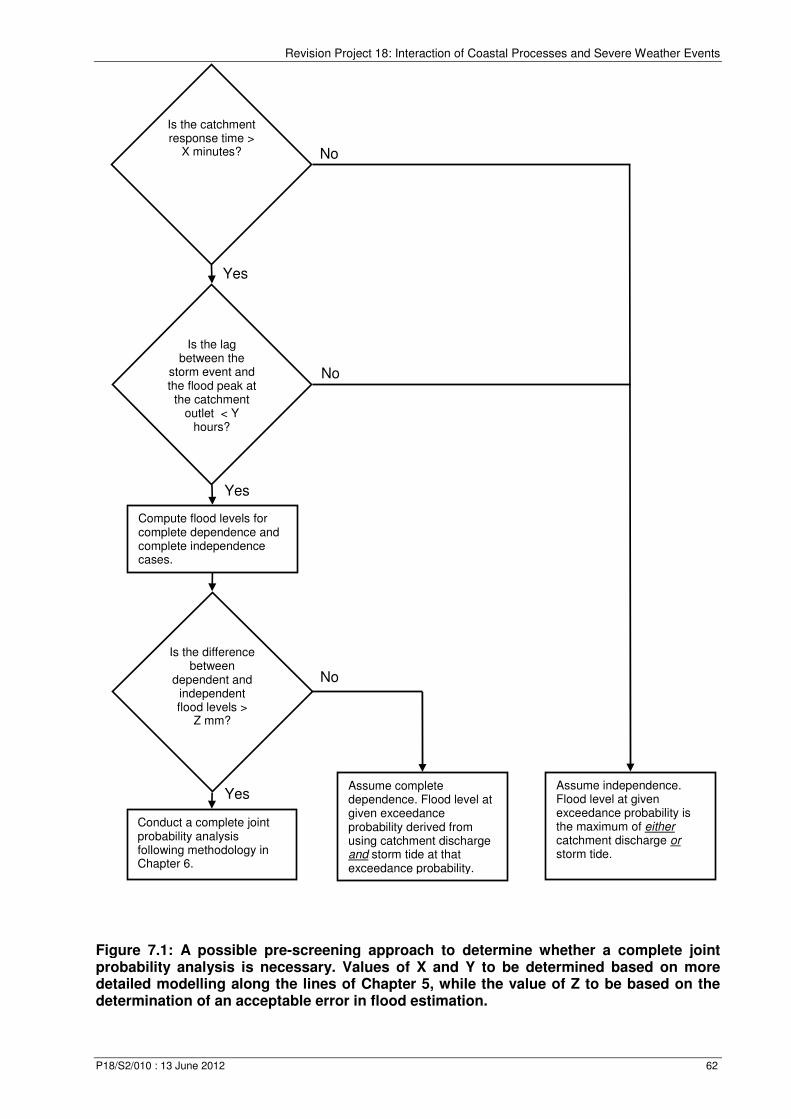
Revision Project 18: Interaction of Coastal Processes and Severe Weather Events
P18/S2/010 : 13 June 2012 62
Is the catchment response time >
X minutes?
Is the lag between the
storm event and the flood peak at the catchment
outlet < Y hours?
Is the difference between
dependent and independent flood levels >
Z mm?
No
Assume independence. Flood level at given exceedance probability is the maximum of either catchment discharge or storm tide.
Compute flood levels for complete dependence and complete independence cases.
Assume complete dependence. Flood level at given exceedance probability derived from using catchment discharge and storm tide at that exceedance probability.
Conduct a complete joint probability analysis following methodology in Chapter 6.
No
Yes
Yes
Yes
No
Figure 7.1: A possible pre-screening approach to determine whether a complete joint probability analysis is necessary. Values of X and Y to be determined based on more detailed modelling along the lines of Chapter 5, while the value of Z to be based on the determination of an acceptable error in flood estimation.
Revision Project 18: Interaction of Coastal Processes and Severe Weather Events
P18/S2/010 : 13 June 2012 63
7.3. Recommendations for further research
In order to complete the guidance required for this section of Australian Rainfall and Runoff, a
range of further research questions were identified. A list of priority research areas is listed
below.
(1) Only a single bivariate extreme value model, namely the bivariate logistic model, was
applied in this study. Although this model provided a reasonable fit to the data for the
higher-dependence cases (e.g. see Figure 4.6, left panel), the model was biased when
the data was actually independent (see Figure 4.7). Additional approaches to modelling
the dependence, along the lines of the models suggested in (Ledford and Tawn, 1996;
Ledford and Tawn, 1997) may be warranted. Kotz and Nadarajah (2000) describe a
range of other bivariate distributions, such as the bilogistic, negative bilogistic, Dirichlet,
Gaussian, circular, Beta, and polynomial distributions, which could be implemented
without too much additional difficulty. Exploration of a broader class of distributions,
including those which do not necessarily fall within the family of bivariate extreme value
distributions, can also be explored (e.g. Favre et al., 2004).
(2) In parallel with this analysis, an empirical review into the largest rainfall and storm surge
events which have occurred at different locations along the Australian coastline could be
conducted, to evaluate the degree to which the most extreme events of both variables
have occurred simultaneously. Both these lines of study are warranted to ensure that the
model performs well under extrapolation, as would be the case for many practical
applications.
(3) The issue of short-term dependence should be taken into account, probably using the
methodology of Coles and Tawn (1991). Provided the ocean level data have been
adequately detrended to account for sea level rise, the issue of non-stationarity at
interannual and longer timescales in both the rainfall and storm surge/tide data is unlikely
to have a large bearing on the results. In contrast the accounting of seasonal variability
could improve the model fit, and further investigation may be warranted.
(4) Having determined the appropriate dependence model(s) for use, these models should
then be applied at all the locations along the Australian coastline for which sufficient data
is available. Given that based on threshold considerations the point-process model used
at least 2 to 3 observations per year, it is possible that the 20-year Australian Baseline
Sea Level Monitoring Project database is sufficiently long for parameter estimation and
thus can be used together with some of the longer records within the 74 stations sourced

Revision Project 18: Interaction of Coastal Processes and Severe Weather Events
P18/S2/010 : 13 June 2012 64
by EngTest (2010). The results of this analysis can be used to evaluate whether there
are any clear patterns associated with the dependence parameter along the Australian
coastline, as well as the degree to which the location of the tide gauge affects the results
(by, for example, comparing the dependence parameters for locations situated along a
river mouth to those situated away from any catchment discharges).
(5) Having fitted the joint dependence model to all gauged locations along the Australian
coastline, the possibility of regionalising the dependence parameter to ungauged
locations will also require exploration. An improved understanding of the principal drivers
of joint dependence will be required for this task. For example, if the dependence is
governed largely by large-scale meteorology, then it may be possible to simulate the
dependence parameter as a smooth function of distance along the Australian coastline.
In contrast, if the dependence parameter varies as a function of local-scale features such
as orientation of the coast or bathymetry, then such factors should also be taken into
consideration in the regionalisation. A hierarchical approach is likely to provide the
simplest method of testing these hypotheses, and is recommended for further
investigation.
(6) Additional historical data beyond the two instrumental records described in this report
may also be available to provide additional information on the nature of joint
dependence, such as the record compiled by Callaghan and Helman (2008). This is
likely to be particularly important given the interest in very large events, since it is not yet
clear how dependence changes as a function of the magnitude of the event, with very
large events potentially exhibiting stronger dependence compared with smaller, more
frequent events. It should be noted that dealing with censored data in the context of
bivariate extremes may be non-trivial, such that methodology may also need to be
developed to properly accommodate such data into the analysis.
(7) To validate the results obtained from examining the rainfall/storm surge data, streamflow
data could be obtained at several locations, and these results compared with the results
derived using the rainfall data described in Chapter 2 of this report.
(8) Several additional case studies are required to implement the approach described in
Chapter 6. The implication for different types of hydrodynamic modelling, including
comparisons with static tail water levels or dynamic tides, should be assessed. The case
studies could also consider a comparison study with continuous simulation or emulation-
based approaches such as described by (Ahmer et al., 2005) to determine the
consistency of results and the relative tradeoffs (in terms of accuracy of flood estimates,
time and effort required for implementation, whether the methods can be extended to
Revision Project 18: Interaction of Coastal Processes and Severe Weather Events
P18/S2/010 : 13 June 2012 65
ungauged locations and so on). Furthermore, guidance on the minimum number of
model runs or the optimal combinations of model runs is required.
Finally, the implications of climate change on the dependence between extreme rainfall and
storm surge can be assessed, potentially using synoptic classification for historical (e.g.
reanalysis) and future (e.g. climate model-derived) climates. The tropical cyclone track data
described in Chapter 2 can also be used to estimate storm surge and rainfall behaviour during
tropical cyclones, which are often the source of some of the most extreme events in northern
Australia; this can then be combined with future projections for the intensity and frequency of
tropical cyclones to estimate how the dependence will change under a future climate. This is
likely to be a much more difficult area of research compared with items 1-5 listed above, and
thus the approximation that the marginal distributions of extreme rainfall and storm tide might
change but that the dependence will stay constant, may be adequate for the forthcoming
revision of Australian Rainfall and Runoff.
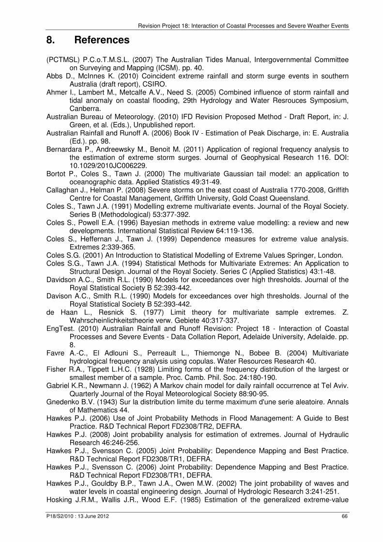
Revision Project 18: Interaction of Coastal Processes and Severe Weather Events
P18/S2/010 : 13 June 2012 66
8. References
(PCTMSL) P.C.o.T.M.S.L. (2007) The Australian Tides Manual, Intergovernmental Committee on Surveying and Mapping (ICSM). pp. 40.
Abbs D., McInnes K. (2010) Coincident extreme rainfall and storm surge events in southern Australia (draft report), CSIRO.
Ahmer I., Lambert M., Metcalfe A.V., Need S. (2005) Combined influence of storm rainfall and tidal anomaly on coastal flooding, 29th Hydrology and Water Resrouces Symposium, Canberra.
Australian Bureau of Meteorology. (2010) IFD Revision Proposed Method - Draft Report, in: J. Green, et al. (Eds.), Unpublished report.
Australian Rainfall and Runoff A. (2006) Book IV - Estimation of Peak Discharge, in: E. Australia (Ed.). pp. 98.
Bernardara P., Andreewsky M., Benoit M. (2011) Application of regional frequency analysis to the estimation of extreme storm surges. Journal of Geophysical Research 116. DOI: 10.1029/2010JC006229.
Bortot P., Coles S., Tawn J. (2000) The multivariate Gaussian tail model: an application to oceanographic data. Applied Statistics 49:31-49.
Callaghan J., Helman P. (2008) Severe storms on the east coast of Australia 1770-2008, Griffith Centre for Coastal Management, Griffith University, Gold Coast Queensland.
Coles S., Tawn J.A. (1991) Modelling extreme multivariate events. Journal of the Royal Society. Series B (Methodological) 53:377-392.
Coles S., Powell E.A. (1996) Bayesian methods in extreme value modelling: a review and new developments. International Statistical Review 64:119-136.
Coles S., Heffernan J., Tawn J. (1999) Dependence measures for extreme value analysis. Extremes 2:339-365.
Coles S.G. (2001) An Introduction to Statistical Modelling of Extreme Values Springer, London. Coles S.G., Tawn J.A. (1994) Statistical Methods for Multivariate Extremes: An Application to
Structural Design. Journal of the Royal Society. Series C (Applied Statistics) 43:1-48. Davidson A.C., Smith R.L. (1990) Models for exceedances over high thresholds. Journal of the
Royal Statistical Society B 52:393-442. Davison A.C., Smith R.L. (1990) Models for exceedances over high thresholds. Journal of the
Royal Statistical Society B 52:393-442. de Haan L., Resnick S. (1977) Limit theory for multivariate sample extremes. Z.
Wahrscheinlichkeitstheorie verw. Gebiete 40:317-337. EngTest. (2010) Australian Rainfall and Runoff Revision: Project 18 - Interaction of Coastal
Processes and Severe Events - Data Collation Report, Adelaide University, Adelaide. pp. 8.
Favre A.-C., El Adlouni S., Perreault L., Thiemonge N., Bobee B. (2004) Multivariate hydrological frequency analysis using copulas. Water Resources Research 40.
Fisher R.A., Tippett L.H.C. (1928) Limiting forms of the frequency distribution of the largest or smallest member of a sample. Proc. Camb. Phil. Soc. 24:180-190.
Gabriel K.R., Newmann J. (1962) A Markov chain model for daily rainfall occurrence at Tel Aviv. Quarterly Journal of the Royal Meteorological Society 88:90-95.
Gnedenko B.V. (1943) Sur la distribution limite du terme maximum d'une serie aleatoire. Annals of Mathematics 44.
Hawkes P.J. (2006) Use of Joint Probability Methods in Flood Management: A Guide to Best Practice. R&D Technical Report FD2308/TR2, DEFRA.
Hawkes P.J. (2008) Joint probability analysis for estimation of extremes. Journal of Hydraulic Research 46:246-256.
Hawkes P.J., Svensson C. (2005) Joint Probability: Dependence Mapping and Best Practice. R&D Technical Report FD2308/TR1, DEFRA.
Hawkes P.J., Svensson C. (2006) Joint Probability: Dependence Mapping and Best Practice. R&D Technical Report FD2308/TR1, DEFRA.
Hawkes P.J., Gouldby B.P., Tawn J.A., Owen M.W. (2002) The joint probability of waves and water levels in coastal engineering design. Journal of Hydrologic Research 3:241-251.
Hosking J.R.M., Wallis J.R., Wood E.F. (1985) Estimation of the generalized extreme-value
Revision Project 18: Interaction of Coastal Processes and Severe Weather Events
P18/S2/010 : 13 June 2012 67
distribution by the method of probability-weighted moments. Technometrics 27:251-261. Joe H., Smith R.L., Weissman I. (1992) Bivariate threshold models for extremes. Journal of the
Royal Statistical Society B 54:171-183. Kalnay E., Kanamitsu M., Ristler R., Collins W., Deaven D., Gandin L., Iredell M., Saha S.,
White G., Woollen J., Zhu Y., Chelliah M., Ebisuzaki W., Higgins W., Janowiak J., Mo K.C., Ropelewski C., Wang J., Leetmaa A., Reynolds R., Jenne R., Joseph D. (1996) The NCEP/NCAR 40-year Reanalysis Project. Bulletin of the American Meteorological Society 77.
Katz R.W., Parlange M.B., Naveau P. (2002) Statistics of extremes in hydrology. Advances in Water Resources 25:18.
Kotz S., Nadarajah S. (2000) Extreme Value Distributions: Theory and Applications Imperial College Press.
Koutsoyiannis D. (2004) Statistics of extremes and estimation of extreme rainfall: I. Theoretical investigation. Hydrological Sciences Journal 49:575-590.
Kuczera G., Lambert M., Heneker T.M., Jennings S., Frost A.J., Coombes P.J. (2006) Joint probability and design storms at the crossroads. Australian Journal of Water Resources 10.
Ledford A.W. (1994) Discussion of paper by S.G. Coles and J.A. Tawn. Applied Statistics 43:41-42.
Ledford A.W., Tawn J.A. (1996) Statistics for near independence in multivariate extreme values. Biometrika 83:169-187.
Ledford A.W., Tawn J.A. (1997) Modelling dependence within joint tail regions. Journal of the Royal Society. Series B (Methodological) 59:475-499.
Loganathan G.V., Kuo C.Y., Yannaccone J. (1987) Joint probability distribution of streamflows and tides in estuaries. Nordic Hydrology 18:237-246.
NSW DECCW. (2009) Draft Flood Risk Management Guide: Incorporating sea level rise benchmarks in flood risk assessments, NSW Department of Environment, Climate Change and Water.
Onogi K., Tsutsui J., Koide H., Sakamoto M., Kobayashi S., Hatsushika H., Matsumoto T., Yamazaki N., HKamahori H., Takahashi K., Kadokura S., Wada K., Kato K., Oyama R., Ose T., Mannoji N., Taira R. (2007) The JRA-25 Reanalysis. Journal of the Meteorological Society of Japan 85:369-432.
Pilgrim D.H. (1987) Australian Rainfall and Runoff, The Institution of Engineers, Australia. Pugh D.T. (1987) Tides, Surges, and Mean Sea-Level, Chichester. Ribatet M., Ouarda T.B.M.J., Sauquet E., Gresillon J.-M. (2009) Modelling all exceedances
above a threshold using an extremal dependence structure: inferences on several flood characteristics. Water Resources Research 45. DOI: 10.1029/2007WR006322.
Saha S., Moorthi S., Pan H.-L., al e. (2010) The NCEP Climate Forecast System Reanalysis. Bulletin of the American Meteorological Society:43. DOI: 10.1175/2010BAMS3001.1.
Smith R.L., Tawn J., Coles S. (1997) Markov chain models for threshold exceedances. Biometrika 84:249-268.
Svensson C., Jones D.A. (2002) Dependence between extreme sea surge, river flow and precipitation in east Britain. International Journal of Climatology 22:1149-1168.
Svensson C., Jones D.A. (2004) Dependence between sea surge, river flow and precipitation in south and west Britain. Hydrological Earth Systems Science 8:973-992.
Svensson C., Jones D.A. (2006) Joint Probability: Dependence between extreme sea surge, river flow and precipitation: A study in South and West Britain. R&D Technical Report FD2308/TR3, DEFRA.
Tawn J. (1988) Bivariate extreme value theory: Models and Estimation. Biometrika 75:397-415. Uppala S.M., KAllberg P.W., Simmons A.J., Andrae U., Da Costa Bechtold V., Fiorino M.,
Gibson J.K., Haseler J., Hernandez A., Kelly G.A., Li X., Onogi K., Saarinen S., Sokka N., Allan R.P., Anderson E., Arpe K., Balmaseda M.A., Beljaars A.C.M., Van de Berg L., Bidlot J., Bormann N., Caires S., Chevallier F., Dethof A., Dragosavac M., Fisher M., Fuentes M., Hagemann S., Holm E., Hoskins B.J., Isaksen L., Janssen P.A.E.M., Jenne R., Mcnally A.P., Mahfouf J.-F., Morcrette J.-J., Rayner N.A., Saunders R.W., Simon P., Sterl A., Trenberth K.E., Untch A., Vasiljevic D., Viterbo P., Woollen J. (2006) The ERA-40 re-analysis. Quarterly Journal of the Royal Meteorological Society 131:2961-3012.
Webb McKeown and Associates. (1996) Warragamba Dam Auxiliary Spillway EIS flood study
Revision Project 18: Interaction of Coastal Processes and Severe Weather Events
P18/S2/010 : 13 June 2012 68
parts A-E. Westra S., Mehrotra R., Sharma A. (2010) Australian Rainfall and Runoff Revision Project 4,
Stage 2: Continuous Rainfall Sequences at a Point Engineers Australia. Yue S., Rasmussen P. (2002) Bivariate frequency analysis: discussion of some useful concepts
in hydrological application. Hydrological Processes 16:2881-2898.

Revision Project 18: Interaction of Coastal Processes and Severe Weather Events
P18/S2/010 : 13 June 2012 69
Appendix 1 – Information on the rain gauges used in the
analysis of Chapter 5.
A1.1: Rain gauges near Fort Denison tide gauge
Table A1: Daily rainfall stations near Fort Denison tide gauge
ID Gauge name Latitude Longitude Distance (km) Start year End year
66006
Sydney Botanic
Gardens -33.8662 151.216
1.59
1885 2009
66062
Sydney Observatory
Hill -33.8607 151.205
2.05
1858 2009
66042
Mosman (Bapaume
Road) -33.8194 151.2428
4.20
1895 2005
66160 Centennial Park -33.8959 151.2341 4.67 1900 2009
66036 Marrickville Golf Club -33.9186 151.1402 10.7 1904 2009
66040 Mirandra -34.0405 151.0982 23.8 1906 2003
66008 Brooklyn -33.5479 151.2079 34.1 1913 2009
68028
Helensburgh (Sawan
St) -34.1908 150.9746
44.0
1889 2005
67015 Bringelly (Maryland) -33.9696 150.725 48.0 1867 2008
68007 Camden -34.0254 150.6455 56.8 1882 2009
63043 Kurrajong Heights -33.5343 150.6338 65.3 1866 2009
61082 Wyee -33.1792 151.4415 77.7 1899 2009
68022 Dapto Bowling Club -34.5 150.7885 82.3 1906 2009
61012
Cooranbong
(Avondale) -33.0853 151.4633
88.3
1903 2009
68009
Burrawang (Range
St) -34.5961 150.5187
105
1891 2009
63036
Oberon (Jenolan
Caves) -33.8199 150.0227
111
1895 2009
63063 Oberon (Springbank) -33.6774 149.8370 130 1888 2009
63032 Golspie (Ayrston) -34.279 149.6651 151 1897 2009
70025 Crookwell PO -34.4578 149.4693 175 1883 2009
61026 Gundy (Miller St) -32.0119 150.9971 206 1887 2009
70112 Dalton Post Office -34.7226 149.1816 211 1899 2009
61097 Moonan Flat -31.9201 151.2355 215 1897 2009
61079 Wingen -31.8679 150.8809 223 1877 2007
65010 Cudal PO -33.2869 148.7396 239 1884 2009
69006 Bettowynd -35.7011 149.7896 244 1897 2009
60023 Harrington -31.8714 152.6827 259 1887 2008
65019 Gooloogong PO -33.6146 148.435 259 1889 2009
55049 Quirindi PO -31.5086 150.6797 266 1882 2009
64026 Cobbora (EllisMayne) -32.0878 149.2349 270 1887 2009
70064 Michelago (Soglio) -35.6797 149.1601 277 1884 2009
69022 Narooma RVCP -36.2144 150.1358 281 1910 2009
65030 Dubbo -32.5192 148.5187 292 1894 2009
64013
Binnaway
(Hawthorne) -31.6417 149.427
298
1886 2009
65012 Dubbo (Darling St) -32.2385 148.6089 303 1870 2009
55004
Bendemeer (Charles
St) -30.8855 151.1533
330
1879 2009
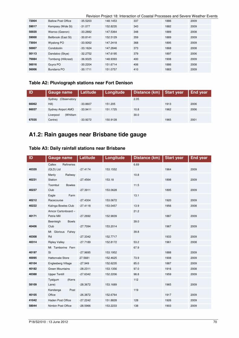
Revision Project 18: Interaction of Coastal Processes and Severe Weather Events
P18/S2/010 : 13 June 2012 70
72004 Batlow Post Office -35.5203 148.1453 337 1886 2009
59017 Kempsey (Wide St) -31.077 152.8235 343 1882 2009
50020 Warroo (Geeron) -33.2882 147.5364 348 1889 2008
59000 Bellbrook (East St) -30.8141 152.5129 359 1889 2009
73054 Wyalong PO -33.9262 147.2418 368 1895 2009
50007 Condobolin -33.1624 147.2846 373 1868 2008
50113 Dandaloo (Skye) -32.2752 147.6195 379 1897 2006
70084 Tombong (Hillcrest) -36.9325 148.9393 400 1908 2009
56016 Guyra PO -30.2204 151.6714 406 1886 2008
56006 Bundarra PO -30.1711 151.0757 410 1883 2009
Table A2: Pluviograph stations near Fort Denison
ID Gauge name Latitude Longitude Distance (km) Start year End year
66062
Sydney (Observatory
Hill) -33.8607 151.205
2.05
1913 2006
66037 Sydney Airport AMO -33.9411 151.1725 10.8 1962 2006
67035
Liverpool (Whitlam
Centre) -33.9272 150.9128
30.0
1965 2001
A1.2: Rain gauges near Brisbane tide gauge
Table A3: Daily rainfall stations near Brisbane
ID Gauge name Latitude Longitude Distance (km) Start year End year
40320
Caltex Refineries
(QLD) Ltd -27.4174 153.1552
6.69
1964 2009
40231
Manly Railway
Station -27.4564 153.18
10.8
1898 2009
40237
Toombul Bowles
Club -27.3911 153.0628
11.5
1895 2009
40212
Eagle Farm
Racecourse -27.4304 153.0672
13.1
1920 2009
40222 Kalinga Bowles Club -27.4118 153.0457 13.9 1956 2008
40171
Amcor Cartonboard –
Petrie Mill -27.2692 152.9839
21.2
1887 2009
40406
Beenleigh Bowls
Club -27.7094 153.2014
39.0
1967 2009
40308
Mt Glorious Fahey
Rd -27.3342 152.7717
39.8
1933 2009
40314 Ripley Valley -27.7189 152.8172 53.2 1961 2008
40197
Mt Tamborine Fern
St -27.9695 153.1952
67.9
1888 2009
40095 Hattonvale Store 27.5681 152.4625 73.9 1908 2009
40104 Englesberg Village -27.949 152.6235 85.0 1887 2009
40182 Green Mountains -28.2311 153.1356 97.0 1916 2008
40388 Upper Tentill -27.6342 152.2206 98.8 1959 2009
58109
Tyalgum (Kerrs
Lane) -28.3672 153.1689
112
1965 2009
40105
Kandanga Post
Office -26.3872 152.6764
119
1917 2009
41042 Haden Post Office -27.2242 151.8828 128 1926 2009
58044 Nimbin Post Office -28.5966 153.2233 138 1903 2009
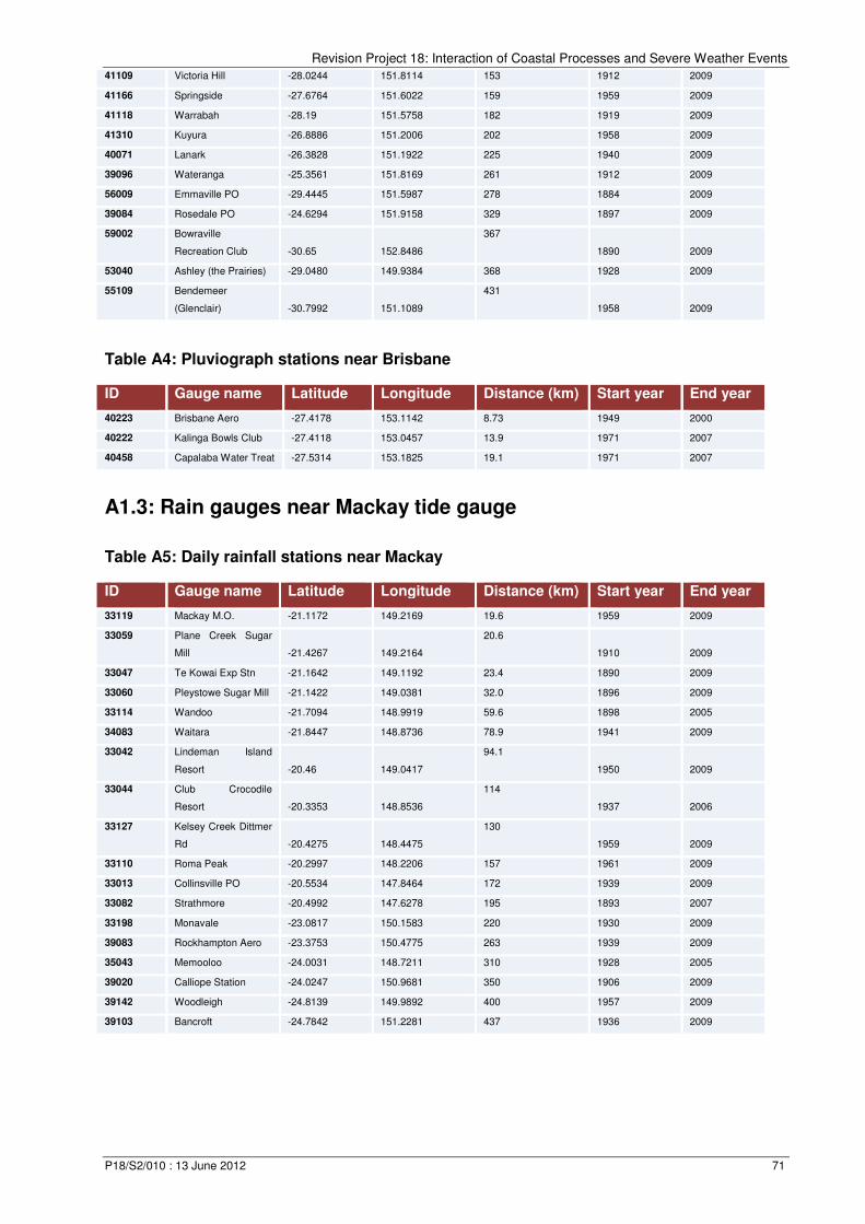
Revision Project 18: Interaction of Coastal Processes and Severe Weather Events
P18/S2/010 : 13 June 2012 71
41109 Victoria Hill -28.0244 151.8114 153 1912 2009
41166 Springside -27.6764 151.6022 159 1959 2009
41118 Warrabah -28.19 151.5758 182 1919 2009
41310 Kuyura -26.8886 151.2006 202 1958 2009
40071 Lanark -26.3828 151.1922 225 1940 2009
39096 Wateranga -25.3561 151.8169 261 1912 2009
56009 Emmaville PO -29.4445 151.5987 278 1884 2009
39084 Rosedale PO -24.6294 151.9158 329 1897 2009
59002 Bowraville
Recreation Club -30.65 152.8486
367
1890 2009
53040 Ashley (the Prairies) -29.0480 149.9384 368 1928 2009
55109 Bendemeer
(Glenclair) -30.7992 151.1089
431
1958 2009
Table A4: Pluviograph stations near Brisbane
ID Gauge name Latitude Longitude Distance (km) Start year End year
40223 Brisbane Aero -27.4178 153.1142 8.73 1949 2000
40222 Kalinga Bowls Club -27.4118 153.0457 13.9 1971 2007
40458 Capalaba Water Treat -27.5314 153.1825 19.1 1971 2007
A1.3: Rain gauges near Mackay tide gauge
Table A5: Daily rainfall stations near Mackay
ID Gauge name Latitude Longitude Distance (km) Start year End year
33119 Mackay M.O. -21.1172 149.2169 19.6 1959 2009
33059 Plane Creek Sugar
Mill -21.4267 149.2164
20.6
1910 2009
33047 Te Kowai Exp Stn -21.1642 149.1192 23.4 1890 2009
33060 Pleystowe Sugar Mill -21.1422 149.0381 32.0 1896 2009
33114 Wandoo -21.7094 148.9919 59.6 1898 2005
34083 Waitara -21.8447 148.8736 78.9 1941 2009
33042 Lindeman Island
Resort -20.46 149.0417
94.1
1950 2009
33044 Club Crocodile
Resort -20.3353 148.8536
114
1937 2006
33127 Kelsey Creek Dittmer
Rd -20.4275 148.4475
130
1959 2009
33110 Roma Peak -20.2997 148.2206 157 1961 2009
33013 Collinsville PO -20.5534 147.8464 172 1939 2009
33082 Strathmore -20.4992 147.6278 195 1893 2007
33198 Monavale -23.0817 150.1583 220 1930 2009
39083 Rockhampton Aero -23.3753 150.4775 263 1939 2009
35043 Memooloo -24.0031 148.7211 310 1928 2005
39020 Calliope Station -24.0247 150.9681 350 1906 2009
39142 Woodleigh -24.8139 149.9892 400 1957 2009
39103 Bancroft -24.7842 151.2281 437 1936 2009
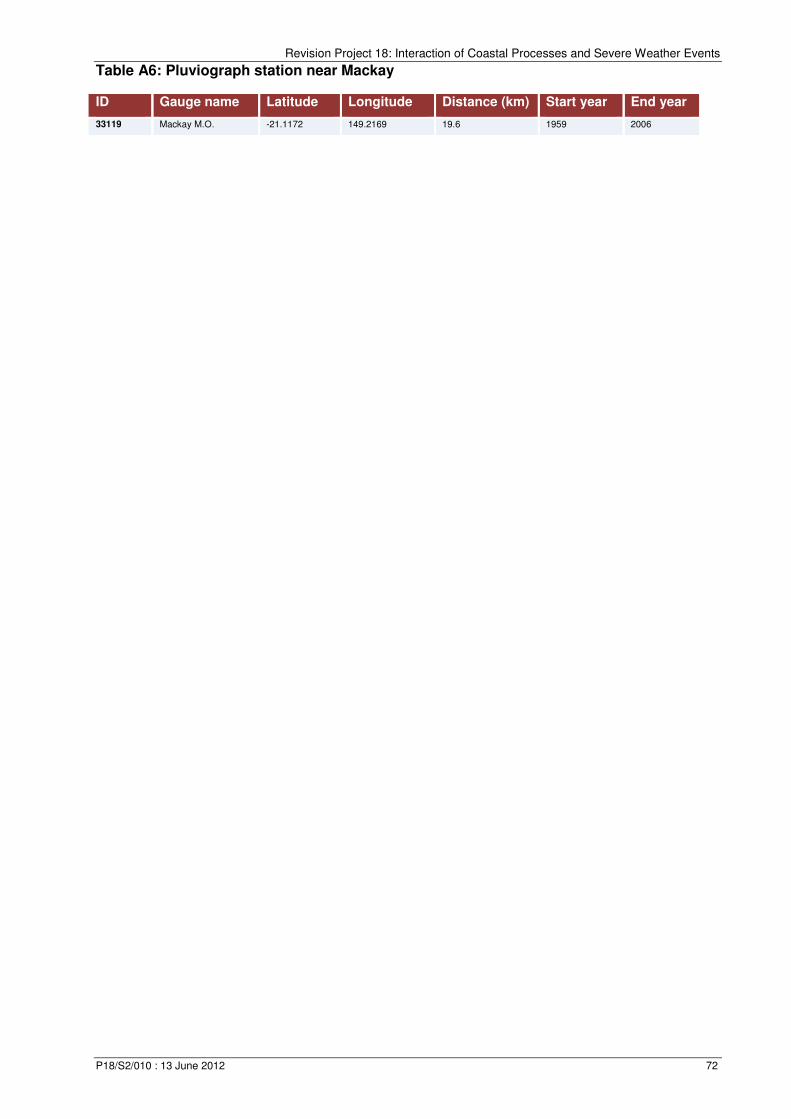
Revision Project 18: Interaction of Coastal Processes and Severe Weather Events
P18/S2/010 : 13 June 2012 72
Table A6: Pluviograph station near Mackay
ID Gauge name Latitude Longitude Distance (km) Start year End year
33119 Mackay M.O. -21.1172 149.2169 19.6 1959 2006