Augmented Split Plot Experiment Design

This article was downloaded by: [139.57.125.60]On: 27 September 2014, At: 18:52Publisher: Taylor & FrancisInforma Ltd Registered in England and Wales Registered Number: 1072954 Registeredoffice: Mortimer House, 37-41 Mortimer Street, London W1T 3JH, UK

Journal of Crop ImprovementPublication details, including instructions for authors andsubscription information:http://www.tandfonline.com/loi/wcim20

Augmented Split Plot Experiment DesignWalter T. Fédérer Jr. a & Florio O. Arguillas ba Department of Biological Statistics and Computational Biology ,Cornell University , Ithaca, NY, 14853, USAb Cornell Institute for Social and Economic Research , CornellUniversity , Ithaca, NY, 14853, USAPublished online: 23 Sep 2008.

To cite this article: Walter T. Fédérer Jr. & Florio O. Arguillas (2006) Augmented Split Plot ExperimentDesign, Journal of Crop Improvement, 15:1, 81-96, DOI: 10.1300/J411v15n01_07

To link to this article: http://dx.doi.org/10.1300/J411v15n01_07

PLEASE SCROLL DOWN FOR ARTICLE

Taylor & Francis makes every effort to ensure the accuracy of all the information (the“Content”) contained in the publications on our platform. However, Taylor & Francis,our agents, and our licensors make no representations or warranties whatsoever as tothe accuracy, completeness, or suitability for any purpose of the Content. Any opinionsand views expressed in this publication are the opinions and views of the authors,and are not the views of or endorsed by Taylor & Francis. The accuracy of the Contentshould not be relied upon and should be independently verified with primary sourcesof information. Taylor and Francis shall not be liable for any losses, actions, claims,proceedings, demands, costs, expenses, damages, and other liabilities whatsoever orhowsoever caused arising directly or indirectly in connection with, in relation to or arisingout of the use of the Content.

This article may be used for research, teaching, and private study purposes. Anysubstantial or systematic reproduction, redistribution, reselling, loan, sub-licensing,systematic supply, or distribution in any form to anyone is expressly forbidden. Terms &Conditions of access and use can be found at http://www.tandfonline.com/page/terms-and-conditions

http://www.tandfonline.com/loi/wcim20

http://www.tandfonline.com/action/showCitFormats?doi=10.1300/J411v15n01_07

http://dx.doi.org/10.1300/J411v15n01_07

http://www.tandfonline.com/page/terms-and-conditions

http://www.tandfonline.com/page/terms-and-conditions

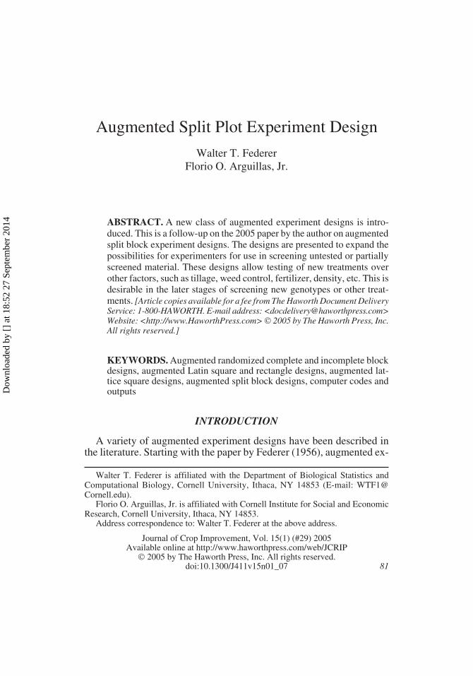
Augmented Split Plot Experiment Design

Walter T. FedererFlorio O. Arguillas, Jr.

ABSTRACT. A new class of augmented experiment designs is intro-duced. This is a follow-up on the 2005 paper by the author on augmentedsplit block experiment designs. The designs are presented to expand thepossibilities for experimenters for use in screening untested or partiallyscreened material. These designs allow testing of new treatments overother factors, such as tillage, weed control, fertilizer, density, etc. This isdesirable in the later stages of screening new genotypes or other treat-ments. [Article copies available for a fee from The Haworth Document DeliveryService: 1-800-HAWORTH. E-mail address: <[email protected]>Website: <http://www.HaworthPress.com> 2005 by The Haworth Press, Inc.All rights reserved.]

KEYWORDS. Augmented randomized complete and incomplete blockdesigns, augmented Latin square and rectangle designs, augmented lat-tice square designs, augmented split block designs, computer codes andoutputs

INTRODUCTION

A variety of augmented experiment designs have been described inthe literature. Starting with the paper by Federer (1956), augmented ex-

Walter T. Federer is affiliated with the Department of Biological Statistics andComputational Biology, Cornell University, Ithaca, NY 14853 (E-mail: [email protected]).

Florio O. Arguillas, Jr. is affiliated with Cornell Institute for Social and EconomicResearch, Cornell University, Ithaca, NY 14853.

Address correspondence to: Walter T. Federer at the above address.

Journal of Crop Improvement, Vol. 15(1) (#29) 2005Available online at http://www.haworthpress.com/web/JCRIP

2005 by The Haworth Press, Inc. All rights reserved.doi:10.1300/J411v15n01_07 81

Dow

nloa

ded

by [

] at

18:

52 2

7 Se

ptem

ber

2014

periment designs were introduced for screening large numbers of geno-types or other treatments, such as herbicides, fungicides, etc. Federer(1961) described augmented complete and incomplete block experi-ment designs. Federer and Raghavarao (1975), Federer et al. (1975),and Federer (1998) presented augmented Latin square designs. In Chap-ter 10 of the Federer (1993) book on intercropping experiments, a pre-sentation of augmented designs is discussed. Federer (2002) presentedthe class of augmented lattice square experiment designs. Computercodes for analyzing data from augmented experiment designs have ap-peared in Federer (2003), Federer and Wolfinger (2003), and Wolfingeret al. (1997). Federer (2005a) has described a class of augmented splitblock designs and analyses for these designs.

The purpose of this paper is to describe how to construct and analyzedata from an augmented split plot experiment design, ASPED, and topresent some variations for this class of designs. In the following sec-tion, a description of an augmented randomized experiment design withsplit plots is given. The statistical analysis is described and is illustratedwith a numerical example.

Under the heading ‘Augmented Genotypes as Split Plots’ the geno-type treatments in an augmented design form the split plot treatments.The statistical analysis is discussed and a numerical example is given toillustrate the procedure. Under the heading ‘Augmented Split-Split PlotExperiment Design,’ the design of ‘Augmented Genotypes as SplitPlots’ with split-split plot treatments is discussed and a statistical analy-sis illustrated with a numerical example is presented. Other variationsare described in the Discussion section. Computer codes are given in thethree appendices.

AUGMENTED GENOTYPES AS WHOLE PLOTS

To illustrate an experiment with augmented genotypes (lines) aswhole plots, consider this example. Suppose there are n new genotypesthat are to be screened for their performances using varying levels ofdensity, irrigation, insecticides, herbicides, or other variables that areused in the growing of a cultivar. These genotypes may have beenscreened in a previous cycle or cycles and have been reduced in number.Consider an augmented randomized complete block experiment designwith r replicates, c standards or checks, n new genotypes with n/r geno-types per replicate. Each of the new genotypes occurs only once in theexperiment.

82 JOURNAL OF CROP IMPROVEMENT

Dow

nloa

ded

by [

] at

18:

52 2

7 Se

ptem

ber

2014

Using a form of a parsimonious experiment design as described byFederer and Scully (1993) and Federer (1993), a whole plot experimen-tal unit, wpeu, would be planted in such a manner that the split plot vari-able has decreasing values throughout the wpeu. For example, supposethat the wpeu is 30 feet long. Then the split plot variable could be ap-plied in decreasing amounts throughout the wpeu. Or, one could parti-tion the wpeu into five, say, split plot experimental units, each being sixfeet in length with either decreasing amounts or in a random allocationmanner of the split plot variable. Certain variables, say density, irriga-tion, herbicide, and fertilizer, lend themselves better to a continuous de-crease. For such a case, there should be no natural gradients within thewpeus. If there is only random variation within a whole plot experimen-tal unit, a systematic application of the split plot treatments from oneend of the experimental unit to the other would not affect the statisticalanalysis as a regression response equation may suffice. It would not beadvisable to have a high level of fertilizer adjacent to a low level unlessthe plots are far enough apart to avoid inter-plot competition.

An analysis of variance table (Table 1) for the above example, maybe of the form.

Example 1

A numerical example is presented to illustrate an analysis for anASPED with genotypes in an augmented randomized complete blockexperiment design and with fertilizer treatments as the split plots. Forthe genotypes, let the number of check genotypes be c = 4 (numbered25-28), the number of new genotypes be n = 24 (numbered 1-24), thenumber of fertilizers be f = 3 (F1, F2, and F3), and the number of repli-cates or blocks be r = 4. Owing to the fact that the SAS procedure (SASInstitute, 1999-2001) sets the highest numbered effect equal to zero, it isa good idea to use the highest number for a check as the estimated ef-fects all have the highest numbered effect subtracted from all other ef-fects, i. e., the effects given by SAS are differences of the effect minusthe highest numbered effect. The standard errors given are standard er-rors of a difference of two effects and not standard errors of an effect asindicated in the output. The responses in Table 2 are fictitious.

The SAS code for the above data is given in Appendix 1. An analysisof variance table, ANOVA, for the responses in Table 1 is presented inTable 3. Type III sums of squares are given. Also presented in the Tableis an ANOVA for checks only and for new treatments only. To obtainthe last two ANOVAs, the SAS code is altered by putting an IF–THEN

Walter T. Federer and Florio O. Arguillas, Jr. 83

Dow

nloa

ded

by [

] at

18:

52 2

7 Se

ptem

ber

2014

statement immediately following the INPUT statement. The statementfor checks only is

IF G < 25 THEN DELETE;

The statement for new genotypes only is

IF G > 24 THEN DELETE;

The MODEL statement for new should be changed to

MODEL Y = F G F*G:

The new treatment effects are confounded with replicate effects.


TABLE 1. Partitioning of the degrees of freedom in an analysis of variance foran augmented split plot experiment.

Source of variation Degrees of freedom

Total f(rc + n)Correction for mean 1Replicates, R r � 1Genotypes, whole plot treatments, G c + n � 1

Checks, C c � 1New, N n � 1C versus N 1

G � R = checks � R = C � R (c � 1)(r � 1)Fertilizer, F f � 1F � G (f � 1)(c + n � 1)

F � C (f � 1)(c � 1)F � N (f � 1)(n � 1)F � C versus N f � 1

F � R within G c(f � 1)(r � 1)

TABLE 2. Responses for ASPED with f = 3, c = 4, n = 24, and r = 4.

Replicate 1 Replicate 2Fert- Genotype Fert- Genotypeilizer 25 26 27 28 1 2 3 4 5 6 ilizer 25 26 27 28 7 8 9 10 11 12

F1 2 1 9 9 2 3 4 5 6 7 F1 3 2 8 7 1 2 3 4 8 3F2 4 3 9 9 5 6 7 8 8 8 F2 3 2 8 8 2 3 4 4 8 5F3 6 5 8 7 7 5 6 4 8 7 F3 7 4 8 9 3 5 4 5 8 7

Replicate 1 Replicate 4Fert- Genotype Fert- Genotypeilizer 25 26 27 28 13 14 15 16 17 18 ilizer 25 26 27 28 19 20 21 22 23 24

F1 4 2 8 7 7 5 3 7 6 5 F1 4 5 9 9 5 6 7 8 9 9F2 6 5 7 7 7 6 5 7 8 7 F2 5 2 9 8 8 6 4 7 8 8F3 8 7 9 9 9 8 6 9 8 8 F2 6 5 9 7 9 8 8 9 9 9

Dow

nloa

ded

by [

] at

18:

52 2

7 Se

ptem

ber

2014

The code for PROC/GLM gives solutions for the parameters in themodel statement and the least squares means (lsmeans) arranged in de-scending order of magnitude. The PROC/MIXED code results in solu-tions for the fixed effects in the model statement, the solutions for therandom effects, the least squares means for the fixed effects in the ordergiven in the lsmeans statement, the random effects solution arranged indescending order, and the lsmeans for fixed effects arranged in de-scending order. If the augmented genotypes are nearing final testing, theexperimenter may wish to consider them as fixed effects. In the earlystages of testing, new genotypes should be considered as random ef-fects. As they near final testing, the survivors become fixed effects witha genotype being given a name.

Since only the check lsmeans and the fertilizer by check lsmeans(Table 4) are estimable by SAS, the estimated effects are presented inTable 5.

In the above analyses, the genotypes effects have been treated asfixed effects. If the analyst wishes to consider them as random effectsand uses the SAS/PROC MIXED procedure, reference may be made tothe codes given in Appendix 1, by Federer (1998, 2003), by Federer andWolfinger (2003), and by Wolfinger et al. (2003). If the number of newgenotypes becomes large, the analyst may wish to order them in de-scending order (see above references) as is done by the computer code


TABLE 3. ANOVA for Example 1, Type III sums of squares.

Source of variation Degrees of freedom Sum of squares Mean square

Total 120 5,181.000Correction for mean 1 4,575.675Replicate, R 3 5.750 1.917Genotype, G 27 343.483 12.722G � R 9 11.750 1.306F 2 50.505 25.252F � G 54 77.983 1.444F � R wn G 24 27.500 1.146

Checks onlyReplicate, R 3 5.750 1.917Check 3 202.417 67.472Check � R 9 11.750 1.306F 2 21.292 10.646F � check 6 21.208 3.535F � R within check 24 27.500 1.146

New onlyNew 23 219.986 9.565F 2 40.444 20.222New � F 46 54.889 1.193

Dow

nloa

ded

by [

] at

18:

52 2

7 Se

ptem

ber

2014

given for this example. Both PROC/GLM and PROC/MIXED analysesare given by the code in Appendix 1.

AUGMENTED GENOTYPES AS SPLIT PLOTS

The genotypes may be used as split plot treatments with whole plottreatments being other factors, such as tillage, fertilizer, irrigation, etc.


TABLE 4. Least squares means for checks and fertilizers for Example 1.

Genotype F1 F2 F3 Genotype

25 3.25 4.50 6.75 4.8326 2.50 3.00 5.25 3.5827 8.50 8.25 8.50 8.4228 8.00 8.00 8.00 8.00

Fertilizer 5.56 5.94 7.06 6.18

TABLE 5. Estimated effects using SAS/GLM for Example 1.

Genotype F1 F2 F3 Genotype

1 �5.00 �2.00 0.00 �1.332 �2.00 +1.00 0.00 �3.333 �2.00 +1.00 0.00 �2.334 +1.00 +4.00 0.00 �4.335 �2.00 0.00 0.00 �0.336 0.00 +1.00 0.00 �1.337 �2.00 �1.00 0.00 �5.008 �3.00 �2.00 0.00 �3.009 �1.00 0.00 0.00 �4.00

10 �1.00 �1.00 0.00 �3.0011 0.00 0.00 0.00 0.0012 �4.00 �2.00 0.00 �1.0013 �2.00 �2.00 0.00 1.3314 �3.00 �2.00 0.00 0.3315 �3.00 �1.00 0.00 �1.6716 �2.00 �2.00 0.00 1.3317 �2.00 0.00 0.00 0.3318 �3.00 �1.00 0.00 0.3319 �4.00 �1.00 0.00 1.0020 �2.00 �2.00 0.00 0.0021 �1.00 �4.00 0.00 0.0022 �1.00 �2.00 0.00 1.0023 0.00 �1.00 0.00 1.0024 0.00 �1.00 0.00 1.0025 �3.50 �2.25 0.00 �1.0826 �2.75 �2.25 0.00 �2.3327 0.00 �0.25 0.00 1.0828 0.00 0.00 0.00 0.00

Fertilizer 0.00 0.00 0.00 0.00

Dow

nloa

ded

by [

] at

18:

52 2

7 Se

ptem

ber

2014

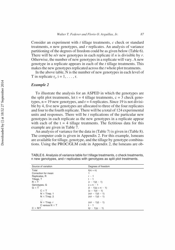
Consider an experiment with t tillage treatments, c check or standardtreatments, n new genotypes, and r replicates. An analysis of variancepartitioning of the degrees of freedom could be as given below (Table 6).There will be n/r new genotypes in each replicate if n is divisible by r.Otherwise, the number of new genotypes in a replicate will vary. A newgenotype in a replicate appears in each of the t tillage treatments. Thismakes the new genotypes replicated across the t whole plot treatments.

In the above table, N is the number of new genotypes in each level ofT in replicate ri, i = 1, . . . , r.

Example 2

To illustrate the analysis for an ASPED in which the genotypes arethe split plot treatments, let t = 4 tillage treatments, c = 3 check geno-types, n = 19 new genotypes, and r = 4 replicates. Since 19 is not divisi-ble by 4, five new genotypes are allocated to three of the four replicatesand four to the fourth replicate. There will be a total of 124 experimentalunits and responses. There will be t replications of the particular newgenotypes in each replicate as the new genotypes in a replicate appearwith each of the t = 4 tillage treatments. The fictitious data for thisexample are given in Table 7.

An analysis of variance for the data in (Table 7) is given in (Table 8).The computer code is given in Appendix 2. For this example, lsmeansare available for tillage, genotype, and the tillage by genotype combina-tions. Using the PROC/GLM code in Appendix 2, the lsmeans are ob-


TABLE 6. Analysis of variance table for t tillage treatments, c check treatments,n new genotypes, and r replicates with genotypes as split plot treatments.


Total t(rc + n)Correction for mean 1Replicates, R r � 1Tillage, T t � 1R � T (r � 1)(t � 1)Genotypes, G c + n � 1G � T (t � 1)(c + n � 1)

C � T (c � 1)(t � 1)N � T/rep. 1 (n/r � 1)(t � 1)N � T/rep. 2 (n/r � 1)(t � 1)…N � T/rep. r (n/r � 1)(t � 1)C versus N � T t � 1

C � R/T t(r � 1)(c � 1)

Dow

nloa

ded

by [

] at

18:

52 2

7 Se

ptem

ber

2014

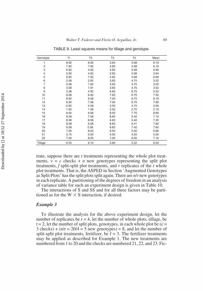
tained in descending order from highest to lowest. The means given inTable 8 are not ordered. The individual analyses of variance for checksalone and for new genotypes alone are not given but may be obtained asdescribed for Example 1.

If the new genotypes are considered to be random effects, use may bemade of the PROC/MIXED part of the code in Appendix 2. Solutionsfor fixed effects in the model statement, solutions for the random effectsin the random statement, lsmeans for the effects in the model statement,a descending order for the fixed effects, a descending order for the ran-dom effects, and a descending order for the fixed effect lsmeans are ob-tained by the code (Table 9).

AUGMENTED SPLIT-SPLIT PLOT EXPERIMENT DESIGN

One of the many variations possible for augmented split plot designsis an augmented split-split plot experiment design, ASSPED. To illus-


TABLE 7. Responses for an ASPED with t = 4, c = 3, r = 4, and n = 19.

Replicate 1 Replicate 2Tillage 20 21 22 1 2 3 4 5 Tillage 20 1 2 6 7 8 9 10

1 6 4 7 8 7 6 5 9 1 8 7 6 3 3 4 4 92 8 5 9 9 8 5 5 8 2 9 6 7 3 2 2 5 73 7 6 9 5 6 7 4 6 3 7 4 5 3 3 3 6 74 5 4 7 3 4 5 2 4 4 6 4 7 5 4 5 7 7

Replicate 3 Replicate 4Tillage 20 21 22 11 12 13 14 15 Tillage 20 21 22 16 17 18 19

1 7 5 8 9 9 1 2 9 1 7 7 7 9 9 9 92 8 3 9 9 7 2 1 9 2 9 6 8 8 9 7 63 6 4 7 7 7 3 2 8 3 6 6 7 7 7 9 94 5 3 6 6 6 4 2 7 4 6 6 6 6 6 7 8

TABLE 8. Type III analysis of variance for responses of Example 2.


Total 124 5,076.000Correction for mean 1 4,512.129Replicate, R 3 4.229 1.410Tillage, T 3 22.668 7.556R � T = error A 9 10.854 1.206Genotype, G 21 309.908 14.758G � T 63 95.140 1.510C � R within T 24 25.167 1.049

Dow

nloa

ded

by [

] at

18:

52 2

7 Se

ptem

ber

2014

trate, suppose there are t treatments representing the whole plot treat-ments, v = c checks + n new genotypes representing the split plottreatments, f split-split plot treatments, and r replicates of the t wholeplot treatments. That is, the ASPED in Section ‘Augmented Genotypesas Split Plots’ has the split plots split again. There are n/r new genotypesin each replicate. A partitioning of the degrees of freedom in an analysisof variance table for such an experiment design is given in Table 10.

The interactions of S and SS and for all three factors may be parti-tioned as for the W � S interaction, if desired.

Example 3

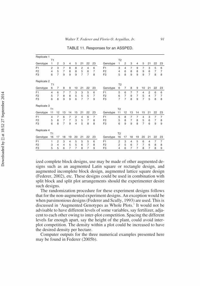
To illustrate the analysis for the above experiment design, let thenumber of replicates be r = 4, let the number of whole plots, tillage, bet = 2, let the number of split plots, genotypes, in each whole plot be (c =3 checks) + (n/r = 20/4 = 5 new genotypes) = 8, and let the number ofsplit-split plot treatments, fertilizer, be f = 3. The fertilizer treatmentsmay be applied as described for Example 1. The new treatments arenumbered from 1 to 20 and the checks are numbered 21, 22, and 23. Fic-


TABLE 9. Least squares means for tillage and genotype.

Genotype T1 T2 T3 T4 Mean

1 8.92 8.92 3.83 3.08 6.192 7.92 7.92 4.83 4.08 6.193 6.92 4.92 5.83 5.08 5.694 5.92 4.92 2.83 2.08 3.945 9.92 7.92 4.83 4.08 6.696 2.58 2.92 3.83 4.75 3.527 2.58 1.92 3.83 3.75 3.028 3.58 1.91 3.83 4.75 3.529 3.38 4.92 6.83 6.75 5.52

10 8.58 6.92 7.83 6.75 7.5211 8.92 9.58 7.50 6.75 8.1912 8.92 7.58 7.50 6.75 7.6913 0.92 2.58 3.50 4.75 2.9414 1.92 1.58 2.50 2.75 2.1915 8.92 9.58 8.50 7.75 8.6916 8.58 7.58 6.83 5.42 7.1017 8.58 8.58 6.83 5.42 7.3518 8.58 6.58 8.83 6.41 7.6019 8.58 5.58 8.83 7.42 7.6020 7.00 8.50 6.50 5.50 6.8821 5.75 5.00 5.00 4.25 5.0022 7.00 8.25 7.00 6.50 7.19

Tillage 6.55 6.10 5.80 5.22 6.03

Dow

nloa

ded

by [

] at

18:

52 2

7 Se

ptem

ber

2014

titious responses for an experiment designed as an augmented split-splitplot experiment design, ASSPED, are given in Table 11.

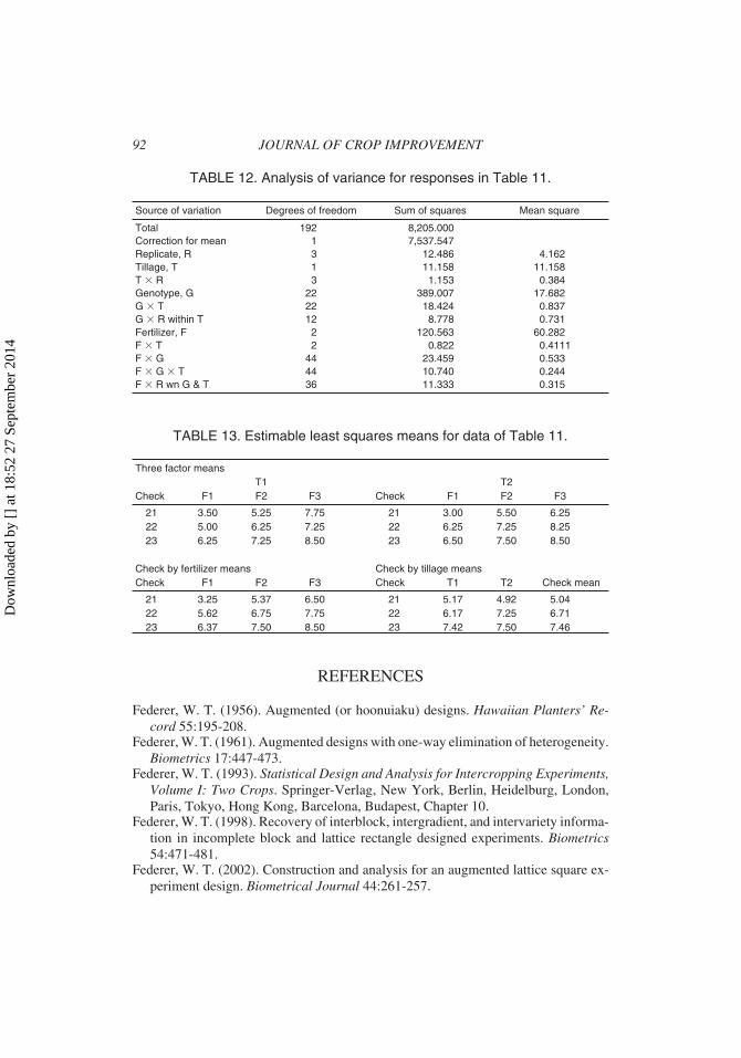
An analysis of variance table for the data in Table 11 is given in Table12. Further partitioning of the degrees of freedom and sums of squaresas described above and for Example 1 may be made here as well.

Only least squares check means are given by SAS. Since lsmeans arenot estimable, solutions for the effects are obtained and are given by thecomputer code in Appendix 3. There are a large number of solutions in-volving all the effects. They may be found in Federer (2005a). Thelsmeans that are estimable are given in Table 13.

DISCUSSION

As indicated, there are many variations of an augmented split plot ex-periment design. Split plot and split block experiment designs in combi-nations may be used if the experimental conditions indicate this. Forexample, an augmented split block design for two factors like tillage, T,and fertilizer, F, could be combined with genotypes, G, as split plots toeither T or F or T and F. F and G could be in a split block arrangement(Federer, 2005) with T as a split plot treatment. Another variation wouldbe to have a split-split-split plot experiment design for T, G, F, and afourth factor, say herbicides, H. Instead of using augmented random-


TABLE 10. Partitioning of the degrees of freedom in an analysis of variance fora split-split plot experiment design.


Total rtcf + tfnCorrection for mean 1Replicate, R r � 1Whole plot treatments, W t � 1R � W = error A (r � 1)(t � 1)Split plot treatments, S v � 1W � S (t � 1)(v � 1)

W � checks, C (t � 1)(c � 1)W � new, N (t � 1)(n � 1)W � C versus N t � 1

S � R within W t(c � 1)(r � 1)Split split plot treatments, SS f � 1SS � W (t � 1)(f � 1)SS � S (f � 1)(v � 1)SS � W � S (f � 1)(v � 1)( t � 1)SS � R within W & S t c(f � 1)(r � 1)

Dow

nloa

ded

by [

] at

18:

52 2

7 Se

ptem

ber

2014

ized complete block designs, use may be made of other augmented de-signs such as an augmented Latin square or rectangle design, andaugmented incomplete block design, augmented lattice square design(Federer, 2002), etc. These designs could be used in combination withsplit block and split plot arrangements should the experimenter desiresuch designs.

The randomization procedure for these experiment designs followsthat for the non-augmented experiment designs. An exception would bewhen parsimonious designs (Federer and Scully, 1993) are used. This isdiscussed in ‘Augmented Genotypes as Whole Plots.’ It would not beadvisable to have different levels of some variables, say fertilizer, adja-cent to each other owing to inter-plot competition. Spacing the differentlevels far enough apart, say the height of the plant, could avoid inter-plot competition. The density within a plot could be increased to havethe desired density per hectare.

Computer outputs for the three numerical examples presented heremay be found in Federer (2005b).


TABLE 11. Responses for an ASSPED.

Replicate 1T1 T2

Genotype 1 2 3 4 5 21 22 23 Genotype 1 2 3 4 5 21 22 23

F1 2 3 7 8 8 2 4 6 F1 3 4 7 9 7 3 5 6F2 4 5 7 8 8 5 6 7 F2 4 6 8 8 9 6 7 7F3 6 7 9 9 9 7 7 8 F3 5 8 9 9 9 7 8 8

Replicate 2T1 T2


F1 4 6 7 7 3 3 5 6 F1 5 6 7 7 4 2 6 6F2 5 7 8 8 5 5 5 7 F2 6 7 9 7 5 4 7 7F3 6 8 9 9 6 7 7 9 F3 7 7 8 9 7 5 8 8

Replicate 3T1 T2


F1 4 7 6 7 2 4 6 7 F1 5 8 7 7 4 3 7 7F2 5 8 7 7 3 5 7 8 F2 5 8 7 8 5 6 7 8F3 6 8 7 9 4 5 8 8 F3 6 9 9 8 7 6 9 9

Replicate 4T1 T2


F1 1 2 3 4 5 5 5 6 F1 2 3 4 5 6 4 7 7F2 3 4 4 5 5 6 7 8 F2 2 5 6 7 7 6 8 8F3 5 5 6 7 7 8 7 9 F3 4 6 7 7 8 7 8 9

Dow

nloa

ded

by [

] at

18:

52 2

7 Se

ptem

ber

2014

REFERENCES

Federer, W. T. (1956). Augmented (or hoonuiaku) designs. Hawaiian Planters’ Re-cord 55:195-208.

Federer, W. T. (1961). Augmented designs with one-way elimination of heterogeneity.Biometrics 17:447-473.

Federer, W. T. (1993). Statistical Design and Analysis for Intercropping Experiments,Volume I: Two Crops. Springer-Verlag, New York, Berlin, Heidelburg, London,Paris, Tokyo, Hong Kong, Barcelona, Budapest, Chapter 10.

Federer, W. T. (1998). Recovery of interblock, intergradient, and intervariety informa-tion in incomplete block and lattice rectangle designed experiments. Biometrics54:471-481.

Federer, W. T. (2002). Construction and analysis for an augmented lattice square ex-periment design. Biometrical Journal 44:261-257.


TABLE 12. Analysis of variance for responses in Table 11.


Total 192 8,205.000Correction for mean 1 7,537.547Replicate, R 3 12.486 4.162Tillage, T 1 11.158 11.158T � R 3 1.153 0.384Genotype, G 22 389.007 17.682G � T 22 18.424 0.837G � R within T 12 8.778 0.731Fertilizer, F 2 120.563 60.282F � T 2 0.822 0.4111F � G 44 23.459 0.533F � G � T 44 10.740 0.244F � R wn G & T 36 11.333 0.315

TABLE 13. Estimable least squares means for data of Table 11.

Three factor meansT1 T2

Check F1 F2 F3 Check F1 F2 F3

21 3.50 5.25 7.75 21 3.00 5.50 6.2522 5.00 6.25 7.25 22 6.25 7.25 8.2523 6.25 7.25 8.50 23 6.50 7.50 8.50

Check by fertilizer means Check by tillage meansCheck F1 F2 F3 Check T1 T2 Check mean

21 3.25 5.37 6.50 21 5.17 4.92 5.0422 5.62 6.75 7.75 22 6.17 7.25 6.7123 6.37 7.50 8.50 23 7.42 7.50 7.46

Dow

nloa

ded

by [

] at

18:

52 2

7 Se

ptem

ber

2014

Federer, W. T. (2003). Analysis for an experiment designed as an augmented latticesquare design. In Handbook of Formulas and Software for Plant Geneticists andBreeders (M. S. Kang, editor), Food Products Press, Binghamton, New York, Chap-ter 27, pp. 283-289.

Federer, W. T. (2005a). Augmented split block experiment design. Agronomy Journal97:578-586.

Federer, W. T. (2005b). Augmented split plot experiment design. BU-1658-M in theTechnical Report Series of the Department of Biological Statistics and Computa-tional Biology (BSCB), Cornell University, Ithaca, NY 14853, June.

Federer, W. T., R. C. Nair, and D. Raghavarao (1975). Some augmented row-columndesigns. Biometrics 31:361-373.

Federer, W. T. and D. Raghavarao (1975). On augmented designs. Biometrics31:29-35.

Federer, W. T. and B. T. Scully (1993). A parsimonious statistical design and breedingprocedure for evaluating and selecting desirable characteristics over environments.Theoretical and Applied Genetics 86:612-620.

Federer, W. T. and R. D. Wolfiger (2003). Augmented row-column designs and trendanalyses. In Handbook of Formulas and Software for Plant Geneticists and Breed-ers (M. S. Kang, editor), Food Products Press, Binghamton, New York, Chapter 28,pp. 291-295.

SAS Institute, Inc. (1999-2001). Release 8.02, copyright, Cary, NC.Wolfinger, R. D., W. T. Federer, and O. Cordero-Brana (1997). Recovering informa-

tion in augmented designs, using SAS PROC GLM and PROC MIXED. AgronomyJournal 89:856-859.


Dow

nloa

ded

by [

] at

18:

52 2

7 Se

ptem

ber

2014

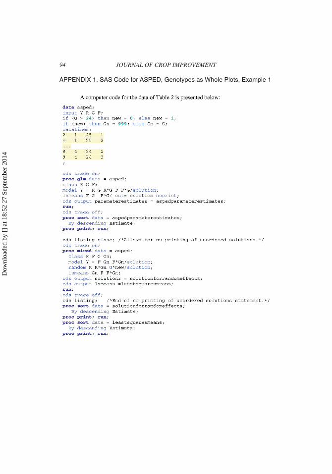
APPENDIX 1. SAS Code for ASPED, Genotypes as Whole Plots, Example 1


Dow

nloa

ded

by [

] at

18:

52 2

7 Se

ptem

ber

2014

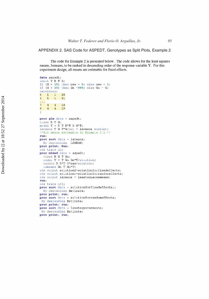
APPENDIX 2. SAS Code for ASPEDT, Genotypes as Split Plots, Example 2


Dow

nloa

ded

by [

] at

18:

52 2

7 Se

ptem

ber

2014

APPENDIX 3. SAS Code for ASSPED, Example 3


Dow

nloa

ded

by [

] at

18:

52 2

7 Se

ptem

ber

2014

Documents

Augmented Split Plot Experiment Design