Embed Size (px)
Citation preview

Aufsätze zur Selbstselektion
und zum Messemanagement
Inauguraldissertation
zur
Erlangung des Doktorgrades
der
Wirtschafts- und Sozialwissenschaftlichen Fakultät
der
Universität zu Köln
2010
vorgelegt
von
Dipl.-Kff. Sabine Scheel-Kopeinig
aus
Villach, Österreich

-II-
Referent: Prof. Dr. Karen Gedenk
Korreferent: Prof. Dr. Franziska Völckner
Tag der Promotion: 23. Juli 2010

-III-
Inhaltsverzeichnis
Abbildungsverzeichnis .................................................................................... VI
Tabellenverzeichnis ......................................................................................... VII
Abkürzungsverzeichnis ................................................................................... VIII
Symbolverzeichnis ........................................................................................... XI
ÜBERBLICK ................................................................................................... 1
Abschnitt A:
Caliendo, Marco/Kopeinig, Sabine: Some Practical Guidance for the
Implementation of Propensity Score Matching ........................................... 6
1. Introduction ..................................................................................................................... A.1
2. Evaluation Framework and Matching Basics ................................................................. A.3
3. Implementation of Propensity Score Matching .............................................................. A.7
3.1 Estimating the Propensity Score ...................................................................................... A.7
3.2 Choosing a Matching Algorithm ..................................................................................... A.11
3.3 Overlap and Common Support ........................................................................................ A.15
3.4 Assessing the Matching Quality ...................................................................................... A.17
3.5 Choice-Based Sampling .................................................................................................. A.19
3.6 When to Compare and Locking-in Effects ....................................................................... A.20
3.7 Estimating the Variance of Treatment Effects .................................................................. A.21
3.8 Combined and Other Propensity Score Methods ............................................................... A.24
3.9 Sensitivity Analysis ........................................................................................................ A.26
3.10 More Practical Issues and Recent Developments .............................................................. A.29
4. Conclusion ...................................................................................................................... A.32
References ........................................................................................................................... A.38

-IV-
Abschnitt B:
Caliendo, Marco/Clement, Michel/Papies, Dominik/Scheel-Kopeinig,
Sabine: The Cost Impact of Spam-Filters: Measuring the Effect of
Information System Technologies in Organizations ................................... 7
Introduction ......................................................................................................................... B.4
Related Research ................................................................................................................. B.8
Method ................................................................................................................................ B.10
Research Design and Data .................................................................................................. B.13
Central Costs ..................................................................................................................... B.14
Individual Measures ........................................................................................................... B.15
Cost Analysis ...................................................................................................................... B.18
Group Characteristics before Matching ............................................................................... B.18
Propensity Score Estimation ............................................................................................... B.18
Matching Results ............................................................................................................... B.20
Effect Heterogeneity .......................................................................................................... B.22
Sensitivity to Unobserved Heterogeneity ............................................................................. B.23
Conclusion and Limitations ................................................................................................ B.25
References ........................................................................................................................... B.27

-V-
Abschnitt C:
Kopeinig, Sabine/Gedenk, Karen: Make-or-Buy-Entscheidungen von
Messegesellschaften ......................................................................................... 8
1. Problemstellung .............................................................................................................. C.3
2. Relevante Make-or-Buy-Fragestellungen ....................................................................... C.5
3. Make-or-Buy-Entscheidungsalternativen ....................................................................... C.7
4. Einflussfaktoren auf die Make-or-Buy-Entscheidung .................................................... C.11
4.1 Einflussfaktoren aus dem Transaktionskostenansatz ......................................................... C.11
4.2 Weitere Einflussfaktoren ................................................................................................ C.15
5. Untersuchung ausgewählter Make-or-Buy-Fragestellungen .......................................... C.17
5.1 Gastronomie-Services ..................................................................................................... C.17
5.2 Standbau-Services .......................................................................................................... C.19
6. Zusammenfassung .......................................................................................................... C.21
Literaturverzeichnis ............................................................................................................ C.22
Literaturverzeichnis ........................................................................................ 9

-VI-
Abbildungsverzeichnis
Abschnitt A
PSM - Implementation Steps ....................................................................................................... A.3
Different Matching Algorithms ................................................................................................... A.11
The Common Support Problem .................................................................................................... A.17
Abschnitt B
Distribution of the Propensity Score. Common Support ............................................................. B.38
Abschnitt C
Wertschöpfungskette einer Messeveranstaltung ......................................................................... C.6
Make-or-Buy-Entscheidungsalternativen .................................................................................... C.8
Grundgedanke des Transaktionskostenansatzes .......................................................................... C.12

-VII-
Tabellenverzeichnis
Überblick
Übersicht der Artikel ................................................................................................................... 1
Abschnitt A
Trade-offs in Terms of Bias and Efficiency ................................................................................ A.14
Implementation of Propensity Score Matching ........................................................................... A.33
Abschnitt B
Central Costs ............................................................................................................................... B.31
Spam-induced Working Time Losses .......................................................................................... B.31
Individual Factors ........................................................................................................................ B.32
Reactance .................................................................................................................................... B.33
Distribution of e-mail addresses ................................................................................................... B.34
Estimation Results of the Logit Model ....................................................................................... B.35
Matching Results .......................................................................................................................... B.36
Group Analysis: Matching Results (group-specific scores) ......................................................... B.36
Sensitivity Analysis, Unobserved Heterogeneity ......................................................................... B.37
Abschnitt C
Services für Messeaussteller und -besucher ................................................................................ C.6
Praxisbeispiele - Entscheidungsalternativen ............................................................................... C.10
Formen der Spezifität ................................................................................................................... C.13
Hypothesen zu Einflussfaktoren des Transaktionskostenansatzes .............................................. C.14
Weitere Einflussfaktoren .............................................................................................................. C.15
Gastronomie-Services .................................................................................................................. C.18
Standbau-Services ........................................................................................................................ C.20

-VIII-
Abkürzungsverzeichnis
ACM Association for Computing Machinery
ATE Average treatment effect
ATT Averate treatment effect of the treated
ATU Averate treatment effect of the untreated
Aufl. Auflage
AUMA Ausstellungs- und Messe-Ausschuss der Deutschen Wirtschaft e.V.
biasaft Standardized bias after matching
biasbef Standardized bias before matching
bzw. beziehungsweise
CIA Conditional independence assumption
Coef. Coefficient
Const. Constant
CS Common support
CVM Covariate matching
DBW Die Betriebswirtschaft (Zeitschrift)
d. h. das heißt
DID Difference-in-differences
DMTP Differentiated mail transfer protocol
eds Editors
e. g. for example
E-mail Electronic mail
Est. Estimator
et al. et alii (und andere)
etc. et cetera
e. V. eingetragener Verein
FAMAB Verband Direkte Wirtschaftskommunikation e.V.
Hrsg. Herausgeber
IFAU Institute for Labour Market Policy Evaluation
IIA Independence for irrelevant alternatives assumption
IS Information systems

-IX-
ISMA International Securities Market Association
ISP Internet service provider
ISR Information Systems Research (Zeitschrift)
IT Information technology
IZA Forschungsinstitut zur Zukunft der Arbeit
Jg. Jahrgang
KM Kernel matching
LLM Local linear matching
LPM Local polynomial matching
MoB Make-or-buy
NCDS National child development study
NN Nearest neighbour
No. Number
Nr. Nummer
NSW National supported work demonstration
Obs. Observations
OECD Organisation for Economic Cooperation and Development
offsup Off support
OLS Ordinary least squares regression
pp pages
PS Propensity score
PSM Propensity score matching
S. Seite
SATT Sample average treatment effect of the treated
SB Standardized bias
s.e. Standard error
SIAW Schweizerisches Institut für Angewandte Wirtschaftsforschung
SPAM Unsolicited bulk messages with commercial content
SUTVA Stable unit treatment value assumption
u. a. und andere
UI Unemployment insurance
vgl. vergleiche

-X-
Vol. Volume
WiSt Wirtschaftswissenschaftliches Studium (Zeitschrift)
www World wide web
z. B. zum Beispiel
ZEW Zentrum Europäische Wirtschaftsforschung GmbH
ZfbF Schmalenbachs Zeitschrift für betriebswirtschaftliche Forschung

-XI-
Symbolverzeichnis
β Coefficient of observable covariates X
b(X) Balancing score
CI+ Upper bound confidence interval
CI- Lower bound confidence interval
D Treatment indicator
E[(.)] Expectation operator
f (.) Nonparametric densitiy estimator
γ Coefficient of unobservable covariates U
k Number of continuous covariates
KM(i) Number of times individual i is used as a match 10λ Mean of Y(1) for individuals outside common support
L Number of options (treatments), with l=1,…,m,…,L
M Number of matches
N Set of individuals, with i=1,…,N
p Polynomial order
P(.) Probability operator
Pr(.) Probability operator
P(X) Propensity Score
P Sample proportion of persons taking treatment
q Treshold amount
σ21(0) Conditional outcome variance
)(ˆ
qPS Region of common support (given a treshold amount q)
Sig+ Upper bound significance level Sig- Lower bound significance level
t-hat+ Upper bound Hodges-Lehmann point estimate
t-hat- Lower bound Hodges-Lehmann point estimate
τi Individual treatment effect
τATE Average treatment effect
τATT Average treatment effect of the treated

-XII-
τSATT Sample average treatment effect of the treated
t Posttreatment period
t’ Pretreatment period
U Unobservable covariates
VarATE Variance bound for ATE
VarATT Variance bound for ATT
VarSATT Variance of sample average treatement effect
Var( ATTτ ) Variance approximation by Lechner
V1[0](X) Variance of X in the treatment [control] group before matching
V1M[0M](X) Variance of X in the treatment [control] group after matching
w(.) Weighting function
X Observable covariates
X 1[1M] Sample average of X in the treatment group before [after] matching
X 0[0M] Sample average of X in the control group before [after] matching
Y Outcome variable
Y(D) Potential outcome given D
Ω Set of the population of interest

-1-
Überblick
Die vorliegende kumulative Dissertation untersucht zwei ausgewählte Problembereiche der
Marketingforschung. Zum einen steht in den Abschnitten A und B die Selbstselektions-
problematik im Fokus. Werden in einem nicht-experimentellen Umfeld kausale Maßnahmen-
effekte ermittelt, können Selbstselektionsverzerrungen auftreten, da eine Zuordnung zur Maß-
nahme nicht zufällig - wie etwa in einem experimentellen Umfeld1 - erfolgt. In Abschnitt A
wird eine Analysemethode im Detail erläutert, die dem Problem der Selbstselektion Rechnung
trägt. In Abschnitt B wird ein Anwendungsbeispiel für diese Methode präsentiert. Zum ande-
ren wird in Abschnitt C eine Make-or-Buy-Fragestellung qualitativ analysiert. Dabei wird der
Frage nachgegangen, ob es für ein Unternehmen profitabler ist, Produkte oder Dienstleistun-
gen selbst zu fertigen bzw. zu erbringen (Make) oder auf dem Markt zu beschaffen (Buy).
In den nachfolgenden Abschnitten A bis C werden die dieser Arbeit zugrundeliegenden drei
Artikel präsentiert. Die nachstehende Tabelle fasst diese Artikel zusammen:
Abschnitt Autoren Titel (Jahr) Zeitschrift/Buch Status
A Marco Caliendo Sabine Kopeinig
Some Practical Guidance for the Implementation of Propensity Score Matching (2008)
Journal of Economic Surveys Publiziert
B
Marco Caliendo Michel Clement Dominik Papies Sabine Scheel-Kopeinig
The Cost Impact of Spam-Filters: Measuring the Effect of Information System Technologies in Organizations (2008)
Information Systems Research (ISR)
Wird in 3. Runde ein-gereicht.
C Sabine Kopeinig Karen Gedenk
Make-or-Buy-Entscheidungen von Messegesellschaften (2005)
Kölner Kompendium der Messewirtschaft Publiziert
Tabelle 1: Übersicht der Artikel
Die Artikel der Abschnitte A Caliendo und Kopeinig (2008) sowie C Kopeinig und Gedenk
(2005) sind in der vorliegenden Form im Journal of Economic Surveys bzw. Kölner Kompen-
dium der Messewirtschaft publiziert. Der Artikel aus Abschnitt B Caliendo/Clement/Papies
und Scheel-Kopeinig (2008) ist als IZA Discussion Paper veröffentlicht. Dieser Artikel befin-
det sich im „editorial process“ und wird in dritter Runde bei der Zeitschrift Information Sys-
tems Research (ISR) eingereicht. Im folgenden Überblick erfolgt eine kurze Zusammen- 1 Vgl. Harrison, G. W./List, J. A. (2004).

-2-
fassung der zentralen Erkenntnisse der oben genannten Artikel unter Darlegung der verfolgten
Zielsetzung und der verwendeten Vorgehensweise.
Die Arbeiten in den Abschnitten A und B behandeln die Selbstselektionsproblematik. Dabei
wird in Caliendo und Kopeinig (2008) eine Analysemethode - Propensity Score Matching
(PSM) - im Detail vorgestellt. In Caliendo/Clement/Papies und Scheel-Kopeinig (2008) wird
ein Anwendungsbeispiel für diese Methode präsentiert. In der empirischen Marketing-
forschung sollen häufig Erfolgswirkungen von Marketingmaßnahmen ermittelt werden. Nicht
immer sind experimentelle Untersuchungsdesigns möglich, um kausale Effekte dieser Maß-
nahmen zu schätzen. Sollen beispielsweise Bonusprogramme oder Messebeteiligungen eva-
luiert werden, muss häufig auf nicht-experimentelle Daten zurückgegriffen werden. Das inhä-
rente Problem der Selbstselektion soll an dem nachfolgenden Beispiel verdeutlicht werden:
Wird der Effekt einer Messeteilnahme lediglich dadurch ermittelt, dass ein Zielgrößenver-
gleich (z. B. Auftragsvolumen) zwischen Messeausstellern und Nichtausstellern erfolgt, dann
wird vernachlässigt, dass unter Umständen gerade erfolgreichere Unternehmen an der Messe
teilnehmen und sich so also „selbst zur Maßnahme selektieren“. Dabei kann die Entscheidung
an der Messe teilzunehmen sowohl von beobachtbaren (z. B. Exportvolumen, Mitarbeiterzahl
der Unternehmen etc.) als auch von unbeobachtbaren Eigenschaften der Unternehmen abhän-
gen. Die zentrale Idee des PSM-Ansatzes2 ist es, aus der Gruppe der Nichtteilnehmer nur jene
Untersuchungseinheiten für den Zielgrößenvergleich heranzuziehen, die den Teilnehmern
bezüglich beobachtbarer Eigenschaften am ähnlichsten sind. Unterschiede in der Zielgröße
zwischen den Teilnehmern an einer Maßnahme und der adjustierten Kontrollgruppe können
dann als Maßnahmeneffekt interpretiert werden.3
Soll ein Maßnahmeneffekt mit Hilfe des Propensity Score Matchings evaluiert werden, ist der
Anwender mit einer Vielzahl an Implementierungsschritten und Detailfragen konfrontiert. In
methodischen Standardwerken4 wird PSM noch nicht besprochen. Daher wird in Caliendo
2 Propensity Score Matching geht zentral auf die Arbeiten von Rubin, D. (1974) sowie Rosenbaum, P./Rubin, D.
(1983b, 1985) zurück. 3 Zentrale Annahme des Matching-Ansatzes ist, dass Unterschiede zwischen Teilnehmern und Nichtteilnehmern
lediglich auf beobachtbaren Eigenschaften beruhen. Diese Annahme ist u. a. als „selection on observables“ be-kannt; vgl. Heckman, J./Robb, R. (1985).
4 Z. B. Backhaus, K./Erichson, B./Plinke, W./Weiber, R. (2008) oder Greene, W. H. (2003).

-3-
und Kopeinig (2008) dem PSM-Anwender ein Leitfaden für die Umsetzung der Implemen-
tierungsschritte und der damit verbundenen Entscheidungen an die Hand gegeben werden.
Nach einer Darstellung des formalen Rahmens wird im Beitrag A gezeigt, wie PSM das
Selbstselektionsproblem lösen kann und welche zentralen Annahmen dazu nötig sind.5 Es
werden fünf zentrale Implementierungsschritte aufgezeigt und mögliche Entscheidungs-
alternativen ausführlich diskutiert. Bei den Implementierungsschritten handelt es sich um die
Schätzung des Propensity Scores (Schritt 1), die Auswahl des Matching-Algorithmus
(Schritt 2), Overlap und Common Support (Schritt 3), Matching Qualität und Schätzung des
Maßnahmeneffektes (Schritt 4) sowie um Sensitivitätsanalysen (Schritt 5). Abschließend
werden noch praxisrelevante Sachverhalte - mit welchen PSM-Anwender konfrontiert sein
können - dargestellt und Weiterentwicklungen des PSM-Ansatzes diskutiert.
Im Ergebnis liefert der vorliegende Beitrag eine bis dato einmalige, anwendungsorientierte,
sequenzielle und gut verständliche Orientierungs- und Entscheidungshilfe bei der PSM-
Implementierung. Außerdem erfolgt eine umfassende Bündelung und Auswertung der wissen-
schaftlichen Literatur zum Thema „Propensity Score Matching“.
Im Beitrag B Caliendo/Clement/Papies und Scheel-Kopeinig (2008) wird analysiert, ob die
Installation eines Spam-Filters die Arbeitszeitverluste von Mitarbeitern, die u. a. dadurch ent-
stehen, dass Spam-Mails überprüft werden müssen, reduzieren kann. Um diesen Maßnahmen-
effekt mit nicht-experimentellen Daten unter Berücksichtigung möglicher Selbstselektions-
verzerrungen zu messen, wird das Verfahren des Propensity Score Matchings angewandt.
Im Zusammenhang mit Spam-Mails entstehen Unternehmen sowohl zentrale Kosten auf IT-
Ebene als auch individuelle Kosten auf Mitarbeiterebene. Sowohl eine Quantifizierung dieser
Kosten als auch eine Analyse der Kostenwirkungen einer Schutzmaßnahme gegen Spam
(Spam-Filter) erfolgte in der wissenschaftlichen Literatur bislang noch nicht. Der vorliegende
Beitrag versucht diese Forschungslücke zu schließen.
5 Vgl. dazu z. B. Heckman, J./Ichimura, H./Todd, P. (1997a).

-4-
Nach einer Zusammenfassung der bisherigen „Spam-Forschung“ und einer kurzen Beschrei-
bung der Methode des Propensity Score Matchings wird die Datenerhebung und das For-
schungsdesign beschrieben und deskriptive Ergebnisse präsentiert. Im Anschluss folgt die
Matchinganalyse. Nach einer Darstellung der Matchingergebnisse werden auch Sensitivitäts-
analysen hinsichtlich Effektheterogentität und unbeobachtbarer Heterogentität durchgeführt.
Der vorliegende Beitrag zeigt, dass Spam-Mails durchaus nennenswerte Kosten auf indivi-
dueller Mitarbeiterebene aber vernachlässigbare Kosten auf IT-Ebene verursachen. Die Instal-
lation eines Spam Filters kann die Arbeitszeitverluste, die Mitarbeitern durch die Kontrolle
und das Löschen von Spam Mails entstehen, um ca. 35 % reduzieren. Die Effektivität der
Schutzmaßnahme hängt aber im Einzelnen maßgeblich von der individuellen Anzahl der er-
haltenen Spam-Mails und vom Spam-Kenntnisstand des Mitarbeiters ab.
Kopeinig und Gedenk (2005) untersuchen im Messe-Kontext die Vorteilhaftigkeit von Make-
or-Buy-(MoB)-Entscheidungen für Messe-Dienstleistungen, wie Gastronomie- oder Stand-
bau-Services. Ziel des Beitrags ist es, Messeunternehmen eine Entscheidungshilfe bei der
Auswahl von möglichen Make-or-Buy-Alternativen an die Hand zu geben. Nach einer Syste-
matisierung relevanter MoB-Entscheidungen von Messegesellschaften werden mögliche
MoB-Entscheidungsalternativen dargestellt. Dabei gibt es zwischen den beiden Extrema
„Make“ und „Buy“ eine Vielzahl relevanter Organisationsformen, bei denen Messe-
gesellschaften mit anderen Unternehmen kooperieren (Cooperate).6 In der Praxis können über
Messegesellschaften und Messe-Dienstleistungen hinweg die gewählten Organisationsformen
erheblich variieren. Beispielsweise werden am Messestandort Frankfurt am Main Gastrono-
mie-Services über ein Tochterunternehmen selbst erbracht. Andere Messegesellschaften favo-
risieren eine marktnahe Alternative und schließen Pachtverträge mit unabhängigen Messe-
gastronomen ab.
Im Beitrag werden Einflussfaktoren auf die Vorteilhaftigkeit der Handlungsalternativen
„Make“ vs. „Buy“ herausgearbeitet. Diese werden zum einen aus dem Transaktionskosten-
ansatz7 und zum anderen aus der konzeptionellen Literatur zum Messewesen abgeleitet. Im
6 Vgl. Picot, A. (1991). 7 Vgl. Coase, R. H. (1937), Williamson, O. E. (1975, 1985).

-5-
speziellen erfolgt eine qualitative Analyse der Vorteilhaftigkeit von „Make“-vs.“Buy“-
Entscheidungen für zwei exemplarische Messe-Dienstleistungen.
Im Ergebnis bietet der vorliegende Beitrag speziell Messeunternehmen eine Entscheidungs-
hilfe für den Entscheidungsprozess „Make-vs.-Buy“ für einzelne Messedienstleistungen. Die
im Fokus der Arbeit stehende Vorgehensweise der Vorteilhaftigkeitsanalyse kann allgemein
auf Make-or-Buy-Fragestellungen in anderen Branchen übertragen werden.

-6-
Abschnitt A:
Caliendo, Marco/Kopeinig, Sabine: Some Practical Guidance for the
Implementation of Propensity Score Matching
Caliendo, Marco/Kopeinig, Sabine: Some Practical Guidance for the Implementation of
Propensity Score Matching, Journal of Economic Surveys, 22. Jg. (1), 2008, S. 31 - 72.

SOME PRACTICAL GUIDANCE FOR THEIMPLEMENTATION OF PROPENSITY
SCORE MATCHING
Marco Caliendo
IZA, Bonn
Sabine Kopeinig
University of Cologne
Abstract. Propensity score matching (PSM) has become a popular approach toestimate causal treatment effects. It is widely applied when evaluating labourmarket policies, but empirical examples can be found in very diverse fields ofstudy. Once the researcher has decided to use PSM, he is confronted with a lot ofquestions regarding its implementation. To begin with, a first decision has to bemade concerning the estimation of the propensity score. Following that one has todecide which matching algorithm to choose and determine the region of commonsupport. Subsequently, the matching quality has to be assessed and treatmenteffects and their standard errors have to be estimated. Furthermore, questions like‘what to do if there is choice-based sampling?’ or ‘when to measure effects?’can be important in empirical studies. Finally, one might also want to test thesensitivity of estimated treatment effects with respect to unobserved heterogeneityor failure of the common support condition. Each implementation step involves alot of decisions and different approaches can be thought of. The aim of this paperis to discuss these implementation issues and give some guidance to researcherswho want to use PSM for evaluation purposes.
Keywords. Propensity score matching; Treatment effects; Evaluation; Sensitivityanalysis; Implementation
1. Introduction
Matching has become a popular approach to estimate causal treatment effects. It iswidely applied when evaluating labour market policies (see e.g., Heckman et al.,1997a; Dehejia and Wahba, 1999), but empirical examples can be found in verydiverse fields of study. It applies for all situations where one has a treatment, agroup of treated individuals and a group of untreated individuals. The nature oftreatment may be very diverse. For example, Perkins et al. (2000) discuss the usage ofmatching in pharmacoepidemiologic research. Hitt and Frei (2002) analyse the effectof online banking on the profitability of customers. Davies and Kim (2003) compare
Journal of Economic Surveys (2008) Vol. 22, No. 1, pp. 31–72C© 2008 The Authors. Journal compilation C© 2008 Blackwell Publishing Ltd, 9600 Garsington Road,Oxford OX4 2DQ, UK and 350 Main Street, Malden, MA 02148, USA.
A.1

32 CALIENDO AND KOPEINIG
the effect on the percentage bid–ask spread of Canadian firms being interlisted on aUS Exchange, whereas Brand and Halaby (2006) analyse the effect of elite collegeattendance on career outcomes. Ham et al. (2004) study the effect of a migrationdecision on the wage growth of young men and Bryson (2002) analyses the effectof union membership on wages of employees. Every microeconometric evaluationstudy has to overcome the fundamental evaluation problem and address the possibleoccurrence of selection bias. The first problem arises because we would like to knowthe difference between the participants’ outcome with and without treatment. Clearly,we cannot observe both outcomes for the same individual at the same time. Takingthe mean outcome of nonparticipants as an approximation is not advisable, sinceparticipants and nonparticipants usually differ even in the absence of treatment.This problem is known as selection bias and a good example is the case wherehigh-skilled individuals have a higher probability of entering a training programmeand also have a higher probability of finding a job. The matching approach is onepossible solution to the selection problem. It originated from the statistical literatureand shows a close link to the experimental context.1 Its basic idea is to find in alarge group of nonparticipants those individuals who are similar to the participants inall relevant pretreatment characteristics X. That being done, differences in outcomesof this well selected and thus adequate control group and of participants can beattributed to the programme. The underlying identifying assumption is known asunconfoundedness, selection on observables or conditional independence. It shouldbe clear that matching is no ‘magic bullet’ that will solve the evaluation problemin any case. It should only be applied if the underlying identifying assumption canbe credibly invoked based on the informational richness of the data and a detailedunderstanding of the institutional set-up by which selection into treatment takesplace (see for example the discussion in Blundell et al., 2005). For the rest of thepaper we will assume that this assumption holds.
Since conditioning on all relevant covariates is limited in the case of a highdimensional vector X (‘curse of dimensionality’), Rosenbaum and Rubin (1983b)suggest the use of so-called balancing scores b(X), i.e. functions of the relevantobserved covariates X such that the conditional distribution of X given b(X) isindependent of assignment into treatment. One possible balancing score is thepropensity score, i.e. the probability of participating in a programme given observedcharacteristics X. Matching procedures based on this balancing score are knownas propensity score matching (PSM) and will be the focus of this paper. Once theresearcher has decided to use PSM, he is confronted with a lot of questions regardingits implementation. Figure 1 summarizes the necessary steps when implementingPSM.2
The aim of this paper is to discuss these issues and give some practical guidanceto researchers who want to use PSM for evaluation purposes. The paper is organizedas follows. In Section 2, we will describe the basic evaluation framework andpossible treatment effects of interest. Furthermore we show how PSM solves theevaluation problem and highlight the implicit identifying assumptions. In Section3, we will focus on implementation steps of PSM estimators. To begin with, afirst decision has to be made concerning the estimation of the propensity score
Journal of Economic Surveys (2008) Vol. 22, No. 1, pp. 31–72C© 2008 The Authors. Journal compilation C© 2008 Blackwell Publishing Ltd
A.2

IMPLEMENTATION OF PROPENSITY SCORE MATCHING 33
Step 0:Decide
between
PSM and
CVM
Step 1:Propensity
Score
Estimation
(Sec. 3.1)
Step 2:Choose
Matching
Algorithm
(Sec. 3.2)
Step 3:Check Over-
lap/Common
Support
(Sec. 3.3)
Step 5:Sensitivity
Analysis
(Sec. 3.9)
Step 4:Matching
Quality/Effect
Estimation(Sec. 3.4-3.8)
Figure 1. PSM – Implementation Steps.
(see Section 3.1). One has not only to decide about the probability model tobe used for estimation, but also about variables which should be included inthis model. In Section 3.2, we briefly evaluate the (dis-)advantages of differentmatching algorithms. Following that we discuss how to check the overlap betweentreatment and comparison group and how to implement the common supportrequirement in Section 3.3. In Section 3.4 we will show how to assess the matchingquality. Subsequently we present the problem of choice-based sampling and discussthe question ‘when to measure programme effects?’ in Sections 3.5 and 3.6.Estimating standard errors for treatment effects will be discussed in Section 3.7before we show in 3.8 how PSM can be combined with other evaluation methods. Thefollowing Section 3.9 is concerned with sensitivity issues, where we first describeapproaches that allow researchers to determine the sensitivity of estimated effectswith respect to a failure of the underlying unconfoundedness assumption. Afterthat we introduce an approach that incorporates information from those individualswho failed the common support restriction, to calculate bounds of the parameterof interest, if all individuals from the sample at hand would have been included.Section 3.10 will briefly discuss the issues of programme heterogeneity, dynamicselection problems, and the choice of an appropriate control group and includes alsoa brief review of the available software to implement matching. Finally, Section 4reviews all steps and concludes.
2. Evaluation Framework and Matching Basics
Roy–Rubin Model
Inference about the impact of a treatment on the outcome of an individual involvesspeculation about how this individual would have performed had (s)he not receivedthe treatment. The standard framework in evaluation analysis to formalize thisproblem is the potential outcome approach or Roy–Rubin model (Roy, 1951; Rubin,1974). The main pillars of this model are individuals, treatment and potentialoutcomes. In the case of a binary treatment the treatment indicator Di equals one ifindividual i receives treatment and zero otherwise. The potential outcomes are thendefined as Yi(Di) for each individual i, where i = 1, . . . , N and N denotes the totalpopulation. The treatment effect for an individual i can be written as
τi = Yi (1) − Yi (0) (1)
Journal of Economic Surveys (2008) Vol. 22, No. 1, pp. 31–72C© 2008 The Authors. Journal compilation C© 2008 Blackwell Publishing Ltd
A.3

34 CALIENDO AND KOPEINIG
The fundamental evaluation problem arises because only one of the potentialoutcomes is observed for each individual i. The unobserved outcome is called thecounterfactual outcome. Hence, estimating the individual treatment effect τ i is notpossible and one has to concentrate on (population) average treatment effects.3
Parameter of Interest and Selection Bias
Two parameters are most frequently estimated in the literature. The first one is thepopulation average treatment effect (ATE), which is simply the difference of theexpected outcomes after participation and nonparticipation:
τATE = E(τ ) = E[Y (1) − Y (0)] (2)
This parameter answers the question: ‘What is the expected effect on the outcome ifindividuals in the population were randomly assigned to treatment?’ Heckman (1997)notes that this estimate might not be of relevance to policy makers because it includesthe effect on persons for whom the programme was never intended. For example,if a programme is specifically targeted at individuals with low family income, thereis little interest in the effect of such a programme for a millionaire. Therefore, themost prominent evaluation parameter is the so-called average treatment effect onthe treated (ATT), which focuses explicitly on the effects on those for whom theprogramme is actually intended. It is given by
τATT = E(τ |D = 1) = E[Y (1)|D = 1] − E[Y (0)|D = 1] (3)
The expected value of ATT is defined as the difference between expected outcomevalues with and without treatment for those who actually participated in treatment.In the sense that this parameter focuses directly on actual treatment participants, itdetermines the realized gross gain from the programme and can be compared with itscosts, helping to decide whether the programme is successful or not (Heckman et al.,1999). The most interesting parameter to estimate depends on the specific evaluationcontext and the specific question asked. Heckman et al. (1999) discuss furtherparameters, like the proportion of participants who benefit from the programmeor the distribution of gains at selected base state values. For most evaluation studies,however, the focus lies on ATT and therefore we will focus on this parameter,too.4 As the counterfactual mean for those being treated – E[Y (0)|D = 1] – is notobserved, one has to choose a proper substitute for it in order to estimate ATT. Usingthe mean outcome of untreated individuals E[Y (0)|D = 0] is in nonexperimentalstudies usually not a good idea, because it is most likely that components whichdetermine the treatment decision also determine the outcome variable of interest.Thus, the outcomes of individuals from the treatment and comparison groups woulddiffer even in the absence of treatment leading to a ‘selection bias’. For ATT it canbe noted as
E[Y (1)|D = 1] − E[Y (0)|D = 0] = τAT T + E[Y (0)|D = 1] − E[Y (0)|D = 0] (4)
Journal of Economic Surveys (2008) Vol. 22, No. 1, pp. 31–72C© 2008 The Authors. Journal compilation C© 2008 Blackwell Publishing Ltd
A.4

IMPLEMENTATION OF PROPENSITY SCORE MATCHING 35
The difference between the left-hand side of equation (4) and τ ATT is the so-called‘selection bias’. The true parameter τ ATT is only identified if
E[Y (0)|D = 1] − E[Y (0)|D = 0] = 0 (5)
In social experiments where assignment to treatment is random this is ensured andthe treatment effect is identified.5 In nonexperimental studies one has to invoke someidentifying assumptions to solve the selection problem stated in equation (4).
Unconfoundedness and Common Support
One major strand of evaluation literature focuses on the estimation of treatmenteffects under the assumption that the treatment satisfies some form of exogene-ity. Different versions of this assumption are referred to as unconfoundedness(Rosenbaum and Rubin, 1983b), selection on observables (Heckman and Robb,1985) or conditional independence assumption (CIA) (Lechner, 1999). We willuse these terms throughout the paper interchangeably. This assumption implies thatsystematic differences in outcomes between treated and comparison individuals withthe same values for covariates are attributable to treatment. Imbens (2004) gives anextensive overview of estimating ATEs under unconfoundedness. The identifyingassumption can be written as
Assumption 1. Unconfoundedness: Y (0), Y (1) � D | X
where � denotes independence, i.e. given a set of observable covariates X whichare not affected by treatment, potential outcomes are independent of treatmentassignment. This implies that all variables that influence treatment assignment andpotential outcomes simultaneously have to be observed by the researcher. Clearly,this is a strong assumption and has to be justified by the data quality at hand. Forthe rest of the paper we will assume that this condition holds. If the researcherbelieves that the available data are not rich enough to justify this assumption, hehas to rely on different identification strategies which explicitly allow selectionon unobservables, too. Prominent examples are difference-in-differences (DID) andinstrumental variables estimators.6 We will show in Section 3.8 how propensity scorematching can be combined with some of these methods.
A further requirement besides independence is the common support or overlapcondition. It rules out the phenomenon of perfect predictability of D given X.
Assumption 2. Overlap: 0 < P(D = 1|X ) < 1.
It ensures that persons with the same X values have a positive probability of beingboth participants and nonparticipants (Heckman et al., 1999). Rosenbaum and Rubin(1983b) call Assumptions 1 and 2 together ‘strong ignorability’. Under ‘strongignorability’ ATE in (2) and ATT in (3) can be defined for all values of X. Heckmanet al. (1998b) demonstrate that the ignorability or unconfoundedness conditions areoverly strong. All that is needed for estimation of (2) and (3) is mean independence.However, Lechner (2002) argues that Assumption 1 has the virtue of identifying
Journal of Economic Surveys (2008) Vol. 22, No. 1, pp. 31–72C© 2008 The Authors. Journal compilation C© 2008 Blackwell Publishing Ltd
A.5

36 CALIENDO AND KOPEINIG
mean effects for all transformations of the outcome variables. The reason is thatthe weaker assumption of mean independence is intrinsically tied to functional formassumptions, making an identification of average effects on transformations of theoriginal outcome impossible (Imbens, 2004). Furthermore, it will be difficult to arguewhy conditional mean independence should hold and Assumption 1 might still beviolated in empirical studies.
If we are interested in estimating the ATT only, we can weaken the unconfound-edness assumption in a different direction. In that case one needs only to assume
Assumption 3. Unconfoundedness for controls: Y (0) � D | X
and the weaker overlap assumption
Assumption 4. Weak overlap: P(D = 1 | X ) < 1.
These assumptions are sufficient for identification of (3), because the moments ofthe distribution of Y (1) for the treated are directly estimable.
Unconfoundedness given the Propensity Score
It should also be clear that conditioning on all relevant covariates is limited inthe case of a high dimensional vector X. For instance if X contains s covariateswhich are all dichotomous, the number of possible matches will be 2s . To dealwith this dimensionality problem, Rosenbaum and Rubin (1983b) suggest usingso-called balancing scores. They show that if potential outcomes are independentof treatment conditional on covariates X, they are also independent of treatmentconditional on a balancing score b(X). The propensity score P(D = 1 | X ) =P(X ), i.e. the probability for an individual to participate in a treatment given hisobserved covariates X, is one possible balancing score. Hence, if Assumption 1holds, all biases due to observable components can be removed by conditioning onthe propensity score (Imbens, 2004).
Corollary 1. Unconfoundedness given the propensity score: Y (0), Y (1)�D | P(X ).7
Estimation Strategy
Given that CIA holds and assuming additionally that there is overlap between bothgroups, the PSM estimator for ATT can be written in general as
τ P SMAT T = EP(X )|D=1{E[Y (1)|D = 1, P(X )] − E[Y (0)|D = 0, P(X )]} (6)
To put it in words, the PSM estimator is simply the mean difference inoutcomes over the common support, appropriately weighted by the propensity scoredistribution of participants. Based on this brief outline of the matching estimator inthe general evaluation framework, we are now going to discuss the implementationof PSM in detail.
Journal of Economic Surveys (2008) Vol. 22, No. 1, pp. 31–72C© 2008 The Authors. Journal compilation C© 2008 Blackwell Publishing Ltd
A.6

IMPLEMENTATION OF PROPENSITY SCORE MATCHING 37
3. Implementation of Propensity Score Matching
3.1 Estimating the Propensity Score
When estimating the propensity score, two choices have to be made. The first oneconcerns the model to be used for the estimation, and the second one the variablesto be included in this model. We will start with the model choice before we discusswhich variables to include in the model.
Model Choice – Binary Treatment
Little advice is available regarding which functional form to use (see for examplethe discussion in Smith, 1997). In principle any discrete choice model can be used.Preference for logit or probit models (compared to linear probability models) derivesfrom the well-known shortcomings of the linear probability model, especially theunlikeliness of the functional form when the response variable is highly skewed andpredictions that are outside the [0, 1] bounds of probabilities. However, when thepurpose of a model is classification rather than estimation of structural coefficients,it is less clear that these criticisms apply (Smith, 1997). For the binary treatmentcase, where we estimate the probability of participation versus nonparticipation, logitand probit models usually yield similar results. Hence, the choice is not too critical,even though the logit distribution has more density mass in the bounds.
Model Choice – Multiple Treatments
However, when leaving the binary treatment case, the choice of the model becomesmore important. The multiple treatment case (as discussed in Imbens (2000) andLechner (2001a)) consists of more than two alternatives, for example when anindividual is faced with the choice to participate in job-creation schemes, vocationaltraining or wage subsidy programmes or to not participate at all (we will describethis approach in more detail in Section 3.10). For that case it is well known thatthe multinomial logit is based on stronger assumptions than the multinomial probitmodel, making the latter the preferable option.8 However, since the multinomialprobit is computationally more burdensome, a practical alternative is to estimate aseries of binomial models as suggested by Lechner (2001a). Bryson et al. (2002)note that there are two shortcomings regarding this approach. First, as the number ofoptions increases, the number of models to be estimated increases disproportionately(for L options we need 0.5(L(L − 1)) models). Second, in each model only twooptions at a time are considered and consequently the choice is conditional on beingin one of the two selected groups. On the other hand, Lechner (2001a) compares theperformance of the multinomial probit approach and series estimation and finds littledifference in their relative performance. He suggests that the latter approach may bemore robust since a mis-specification in one of the series will not compromise allothers as would be the case in the multinomial probit model.
Journal of Economic Surveys (2008) Vol. 22, No. 1, pp. 31–72C© 2008 The Authors. Journal compilation C© 2008 Blackwell Publishing Ltd
A.7

38 CALIENDO AND KOPEINIG
Variable Choice:
More advice is available regarding the inclusion (or exclusion) of covariates inthe propensity score model. The matching strategy builds on the CIA, requiringthat the outcome variable(s) must be independent of treatment conditional on thepropensity score. Hence, implementing matching requires choosing a set of variablesX that credibly satisfy this condition. Heckman et al. (1997a) and Dehejia and Wahba(1999) show that omitting important variables can seriously increase bias in resultingestimates. Only variables that influence simultaneously the participation decisionand the outcome variable should be included. Hence, economic theory, a soundknowledge of previous research and also information about the institutional settingsshould guide the researcher in building up the model (see e.g., Sianesi, 2004; Smithand Todd, 2005). It should also be clear that only variables that are unaffected byparticipation (or the anticipation of it) should be included in the model. To ensurethis, variables should either be fixed over time or measured before participation. Inthe latter case, it must be guaranteed that the variable has not been influenced bythe anticipation of participation. Heckman et al. (1999) also point out that the datafor participants and nonparticipants should stem from the same sources (e.g. thesame questionnaire). The better and more informative the data are, the easier it isto credibly justify the CIA and the matching procedure. However, it should also beclear that ‘too good’ data is not helpful either. If P(X ) = 0 or P(X ) = 1 for somevalues of X, then we cannot use matching conditional on those X values to estimatea treatment effect, because persons with such characteristics either always or neverreceive treatment. Hence, the common support condition as stated in Assumption 2fails and matches cannot be performed. Some randomness is needed that guaranteesthat persons with identical characteristics can be observed in both states (Heckmanet al., 1998b).
In cases of uncertainty of the proper specification, sometimes the question mayarise whether it is better to include too many rather than too few variables. Brysonet al. (2002) note that there are two reasons why over-parameterized models shouldbe avoided. First, it may be the case that including extraneous variables in theparticipation model exacerbates the support problem. Second, although the inclusionof nonsignificant variables in the propensity score specification will not bias thepropensity score estimates or make them inconsistent, it can increase their variance.
The results from Augurzky and Schmidt (2001) point in the same direction.They run a simulation study to investigate PSM when selection into treatment isremarkably strong, and treated and untreated individuals differ considerably in theirobservable characteristics. In their set-up, explanatory variables in the selectionequation are partitioned into three sets. The first set (set 1) includes covariateswhich strongly influence the treatment decision but weakly influence the outcomevariable. Furthermore, they include covariates which are relevant to the outcomebut irrelevant to the treatment decision (set 2) and covariates which influence both(set 3). Including the full set of covariates in the propensity score specification (fullmodel including all three sets of covariates) might cause problems in small samplesin terms of higher variance, since either some treated have to be discarded from the
Journal of Economic Surveys (2008) Vol. 22, No. 1, pp. 31–72C© 2008 The Authors. Journal compilation C© 2008 Blackwell Publishing Ltd
A.8

IMPLEMENTATION OF PROPENSITY SCORE MATCHING 39
analysis or control units have to be used more than once. They show that matchingon an inconsistent estimate of the propensity score (i.e. partial model including onlyset 3 or both sets 1 and 3) produces better estimation results of the ATE.
On the other hand, Rubin and Thomas (1996) recommend against ‘trimming’models in the name of parsimony. They argue that a variable should only be excludedfrom analysis if there is consensus that the variable is either unrelated to the outcomeor not a proper covariate. If there are doubts about these two points, they explicitlyadvise to include the relevant variables in the propensity score estimation.
By these criteria, there are both reasons for and against including all of thereasonable covariates available. Basically, the points made so far imply that thechoice of variables should be based on economic theory and previous empiricalfindings. But clearly, there are also some formal (statistical) tests which can beused. Heckman et al. (1998a), Heckman and Smith (1999) and Black and Smith(2004) discuss three strategies for the selection of variables to be used in estimatingthe propensity score.
Hit or Miss Method
The first one is the ‘hit or miss’ method or prediction rate metric, where variablesare chosen to maximize the within-sample correct prediction rates. This methodclassifies an observation as ‘1’ if the estimated propensity score is larger thanthe sample proportion of persons taking treatment, i.e. P(X ) > P . If P(X ) ≤ Pobservations are classified as ‘0’. This method maximizes the overall classificationrate for the sample assuming that the costs for the misclassification are equal forthe two groups (Heckman et al., 1997a).9 But clearly, it has to be kept in mind thatthe main purpose of the propensity score estimation is not to predict selection intotreatment as well as possible but to balance all covariates (Augurzky and Schmidt,2001).
Statistical Significance
The second approach relies on statistical significance and is very common intextbook econometrics. To do so, one starts with a parsimonious specification ofthe model, e.g. a constant, the age and some regional information, and then ‘testsup’ by iteratively adding variables to the specification. A new variable is kept ifit is statistically significant at conventional levels. If combined with the ‘hit ormiss’ method, variables are kept if they are statistically significant and increase theprediction rates by a substantial amount (Heckman et al., 1998a).
Leave-One-Out Cross-Validation
Leave-one-out cross-validation can also be used to choose the set of variablesto be included in the propensity score. Black and Smith (2004) implement theirmodel selection procedure by starting with a ‘minimal’ model containing only twovariables. They subsequently add blocks of additional variables and compare the
Journal of Economic Surveys (2008) Vol. 22, No. 1, pp. 31–72C© 2008 The Authors. Journal compilation C© 2008 Blackwell Publishing Ltd
A.9

40 CALIENDO AND KOPEINIG
resulting mean squared errors. As a note of caution, they stress that this amountsto choosing the propensity score model based on goodness-of-fit considerations,rather than based on theory and evidence about the set of variables related to theparticipation decision and the outcomes (Black and Smith, 2004). They also pointout an interesting trade-off in finite samples between the plausibility of the CIA andthe variance of the estimates. When using the full specification, bias arises fromselecting a wide bandwidth in response to the weakness of the common support.In contrast to that, when matching on the minimal specification, common supportis not a problem but the plausibility of the CIA is. This trade-off also affects theestimated standard errors, which are smaller for the minimal specification where thecommon support condition poses no problem.
Finally, checking the matching quality can also help to determine the propensityscore specification and we will discuss this point later in Section 3.4.
Overweighting some Variables
Let us assume for the moment that we have found a satisfactory specificationof the model. It may sometimes be felt that some variables play a specificallyimportant role in determining participation and outcome (Bryson et al., 2002). Asan example, one can think of the influence of gender and region in determiningthe wage of individuals. Let us take as given for the moment that men earn morethan women and the wage level is higher in region A compared to region B. If weadd dummy variables for gender and region in the propensity score estimation, it isstill possible that women in region B are matched with men in region A, since thegender and region dummies are only a subset of all available variables. There arebasically two ways to put greater emphasis on specific variables. One can either findvariables in the comparison group who are identical with respect to these variables,or carry out matching on subpopulations. The study from Lechner (2002) is a goodexample for the first approach. He evaluates the effects of active labour marketpolicies in Switzerland and uses the propensity score as a ‘partial’ balancing scorewhich is complemented by an exact matching on sex, duration of unemploymentand native language. Heckman et al. (1997a, 1998a) use the second strategy andimplement matching separately for four demographic groups. That implies that thecomplete matching procedure (estimating the propensity score, checking the commonsupport, etc.) has to be implemented separately for each group. This is analogous toinsisting on a perfect match, e.g. in terms of gender and region, and then carryingout propensity score matching. This procedure is especially recommendable if oneexpects the effects to be heterogeneous between certain groups.
Alternatives to the Propensity Score
Finally, it should also be noted that it is possible to match on a measure otherthan the propensity score, namely the underlying index of the score estimation.The advantage of this is that the index differentiates more between observationsin the extremes of the distribution of the propensity score (Lechner, 2000). This is
Journal of Economic Surveys (2008) Vol. 22, No. 1, pp. 31–72C© 2008 The Authors. Journal compilation C© 2008 Blackwell Publishing Ltd
A.10

IMPLEMENTATION OF PROPENSITY SCORE MATCHING 41
Matching Algorithms
Nearest
Neighbour (NN)
Caliper and Radius
Stratification and
Interval
Kernel and Local
Linear
With/without replacementOversampling (2-NN, 5-NN a.s.o.)Weights for oversampling
Max. tolerance level (caliper)1-NN only or more (radius)
Number of strata/intervals
Kernel functions (e.g. Gaussian, a.s.o.)Bandwidth parameter
Figure 2. Different Matching Algorithms.
useful if there is some concentration of observations in the tails of the distribution.Additionally, in some recent papers the propensity score is estimated by durationmodels. This is of particular interest if the ‘timing of events’ plays a crucial role(see e.g. Brodaty et al., 2001; Sianesi, 2004).
3.2 Choosing a Matching Algorithm
The PSM estimator in its general form was stated in equation (6). All matchingestimators contrast the outcome of a treated individual with outcomes of comparisongroup members. PSM estimators differ not only in the way the neighbourhood foreach treated individual is defined and the common support problem is handled,but also with respect to the weights assigned to these neighbours. Figure 2 depictsdifferent PSM estimators and the inherent choices to be made when they are used.We will not discuss the technical details of each estimator here at depth but ratherpresent the general ideas and the involved trade-offs with each algorithm.10
Nearest Neighbour Matching
The most straightforward matching estimator is nearest neighbour (NN) matching.The individual from the comparison group is chosen as a matching partner for atreated individual that is closest in terms of the propensity score. Several variantsof NN matching are proposed, e.g. NN matching ‘with replacement’ and ‘withoutreplacement’. In the former case, an untreated individual can be used more thanonce as a match, whereas in the latter case it is considered only once. Matching withreplacement involves a trade-off between bias and variance. If we allow replacement,the average quality of matching will increase and the bias will decrease. This is of
Journal of Economic Surveys (2008) Vol. 22, No. 1, pp. 31–72C© 2008 The Authors. Journal compilation C© 2008 Blackwell Publishing Ltd
A.11

42 CALIENDO AND KOPEINIG
particular interest with data where the propensity score distribution is very differentin the treatment and the control group. For example, if we have a lot of treatedindividuals with high propensity scores but only few comparison individuals withhigh propensity scores, we get bad matches as some of the high-score participantswill get matched to low-score nonparticipants. This can be overcome by allowingreplacement, which in turn reduces the number of distinct nonparticipants usedto construct the counterfactual outcome and thereby increases the variance of theestimator (Smith and Todd, 2005). A problem which is related to NN matchingwithout replacement is that estimates depend on the order in which observationsget matched. Hence, when using this approach it should be ensured that ordering israndomly done.11
It is also suggested to use more than one NN (‘oversampling’). This form ofmatching involves a trade-off between variance and bias, too. It trades reducedvariance, resulting from using more information to construct the counterfactual foreach participant, with increased bias that results from on average poorer matches(see e.g. Smith, 1997). When using oversampling, one has to decide how manymatching partners should be chosen for each treated individual and which weight(e.g. uniform or triangular weight) should be assigned to them.
Caliper and Radius Matching
NN matching faces the risk of bad matches if the closest neighbour is far away. Thiscan be avoided by imposing a tolerance level on the maximum propensity scoredistance (caliper). Hence, caliper matching is one form of imposing a commonsupport condition (we will come back to this point in Section 3.3). Bad matches areavoided and the matching quality rises. However, if fewer matches can be performed,the variance of the estimates increases.12 Applying caliper matching means that anindividual from the comparison group is chosen as a matching partner for a treatedindividual that lies within the caliper (‘propensity range’) and is closest in terms ofpropensity score. As Smith and Todd (2005) note, a possible drawback of calipermatching is that it is difficult to know a priori what choice for the tolerance levelis reasonable.
Dehejia and Wahba (2002) suggest a variant of caliper matching which is calledradius matching. The basic idea of this variant is to use not only the NN withineach caliper but all of the comparison members within the caliper. A benefit of thisapproach is that it uses only as many comparison units as are available within thecaliper and therefore allows for usage of extra (fewer) units when good matches are(not) available. Hence, it shares the attractive feature of oversampling mentionedabove, but avoids the risk of bad matches.
Stratification and Interval Matching
The idea of stratification matching is to partition the common support of thepropensity score into a set of intervals (strata) and to calculate the impact withineach interval by taking the mean difference in outcomes between treated and
Journal of Economic Surveys (2008) Vol. 22, No. 1, pp. 31–72C© 2008 The Authors. Journal compilation C© 2008 Blackwell Publishing Ltd
A.12

IMPLEMENTATION OF PROPENSITY SCORE MATCHING 43
control observations. This method is also known as interval matching, blockingand subclassification (Rosenbaum and Rubin, 1984). Clearly, one question tobe answered is how many strata should be used in empirical analysis. Cochran(1968) shows that five subclasses are often enough to remove 95% of the biasassociated with one single covariate. Since, as Imbens (2004) notes, all bias underunconfoundedness is associated with the propensity score, this suggests that undernormality the use of five strata removes most of the bias associated with allcovariates. One way to justify the choice of the number of strata is to check thebalance of the propensity score (or the covariates) within each stratum (see e.g.Aakvik, 2001). Most of the algorithms can be described in the following way.First, check if within a stratum the propensity score is balanced. If not, strataare too large and need to be split. If, conditional on the propensity score beingbalanced, the covariates are unbalanced, the specification of the propensity scoreis not adequate and has to be respecified, e.g. through the addition of higher-orderterms or interactions (see Dehejia and Wahba, 1999; Dehejia, 2005).
Kernel and Local Linear Matching
The matching algorithms discussed so far have in common that only a fewobservations from the comparison group are used to construct the counterfactualoutcome of a treated individual. Kernel matching (KM) and local linear matching(LLM) are nonparametric matching estimators that use weighted averages of (nearly)all – depending on the choice of the kernel function – individuals in the controlgroup to construct the counterfactual outcome. Thus, one major advantage of theseapproaches is the lower variance which is achieved because more information isused. A drawback of these methods is that possibly observations are used that arebad matches. Hence, the proper imposition of the common support condition is ofmajor importance for KM and LLM. Heckman et al. (1998b) derive the asymptoticdistribution of these estimators and Heckman et al. (1997a) present an application.As Smith and Todd (2005) note, KM can be seen as a weighted regression of thecounterfactual outcome on an intercept with weights given by the kernel weights.Weights depend on the distance between each individual from the control groupand the participant observation for which the counterfactual is estimated. It is worthnoting that if weights from a symmetric, nonnegative, unimodal kernel are used, thenthe average places higher weight on persons close in terms of the propensity scoreof a treated individual and lower weight on more distant observations. The estimatedintercept provides an estimate of the counterfactual mean. The difference betweenKM and LLM is that the latter includes in addition to the intercept a linear term in thepropensity score of a treated individual. This is an advantage whenever comparisongroup observations are distributed asymmetrically around the treated observation,e.g. at boundary points, or when there are gaps in the propensity score distribution.When applying KM one has to choose the kernel function and the bandwidthparameter. The first point appears to be relatively unimportant in practice (DiNardoand Tobias, 2001). What is seen as more important (see e.g. Silverman, 1986;Pagan and Ullah, 1999) is the choice of the bandwidth parameter with the following
Journal of Economic Surveys (2008) Vol. 22, No. 1, pp. 31–72C© 2008 The Authors. Journal compilation C© 2008 Blackwell Publishing Ltd
A.13

44 CALIENDO AND KOPEINIG
Table 1. Trade-offs in Terms of Bias and Efficiency.
Decision Bias Variance
Nearest neighbour matching:multiple neighbours/single neighbour (+)/(−) (−)/(+)with caliper/without caliper (−)/(+) (+)/(−)
Use of control individuals:with replacement/without replacement (−)/(+) (+)/(−)
Choosing method:NN matching/Radius matching (−)/(+) (+)/(−)KM or LLM/NN methods (+)/(−) (−)/(+)
Bandwidth choice with KM:small/large (−)/(+) (+)/(−)
Polynomial order with LPM:small/large (+)/(−) (−)/(+)
KM, kernel matching, LLM; local linear matching; LPM, local polynomial matching NN, nearestneighbour; increase; (+); decrease (−).
trade-off arising. High bandwidth values yield a smoother estimated density function,therefore leading to a better fit and a decreasing variance between the estimated andthe true underlying density function. On the other hand, underlying features may besmoothed away by a large bandwidth leading to a biased estimate. The bandwidthchoice is therefore a compromise between a small variance and an unbiased estimateof the true density function. It should be noted that LLM is a special case of localpolynomial matching (LPM). LPM includes in addition to an intercept a term ofpolynomial order p in the propensity score, e.g. p = 1 for LLM, p = 2 for localquadratic matching or p = 3 for local cubic matching. Generally, the larger thepolynomial order p is the smaller will be the asymptotic bias but the larger will bethe asymptotic variance. To our knowledge Ham et al. (2004) is the only applicationof local cubic matching so far, and hence practical experiences with LPM estimatorswith p ≥ 2 are rather limited.
Trade-offs in Terms of Bias and Efficiency
Having presented the different possibilities, the question remains of how one shouldselect a specific matching algorithm. Clearly, asymptotically all PSM estimatorsshould yield the same results, because with growing sample size they all becomecloser to comparing only exact matches (Smith, 2000). However, in small samples thechoice of the matching algorithm can be important (Heckman et al., 1997a), whereusually a trade-off between bias and variance arises (see Table 1). So what advicecan be given to researchers facing the problem of choosing a matching estimator? It
Journal of Economic Surveys (2008) Vol. 22, No. 1, pp. 31–72C© 2008 The Authors. Journal compilation C© 2008 Blackwell Publishing Ltd
A.14

IMPLEMENTATION OF PROPENSITY SCORE MATCHING 45
should be clear that there is no ‘winner’ for all situations and that the choice of theestimator crucially depends on the situation at hand. The performance of differentmatching estimators varies case-by-case and depends largely on the data structure athand (Zhao, 2000). To give an example, if there are only a few control observations,it makes no sense to match without replacement. On the other hand, if there are alot of comparable untreated individuals it might be worth using more than one NN(either by oversampling or KM) to gain more precision in estimates. Pragmatically,it seems sensible to try a number of approaches. Should they give similar results,the choice may be unimportant. Should results differ, further investigation may beneeded in order to reveal more about the source of the disparity (Bryson et al.,2002).
3.3 Overlap and Common Support
Our discussion in Section 2 has shown that ATT and ATE are only defined in theregion of common support. Heckman et al. (1997a) point out that a violation of thecommon support condition is a major source of evaluation bias as conventionallymeasured. Comparing the incomparable must be avoided, i.e. only the subset of thecomparison group that is comparable to the treatment group should be used in theanalysis (Dehejia and Wahba, 1999). Hence, an important step is to check the overlapand the region of common support between treatment and comparison group. Severalways are suggested in the literature, where the most straightforward one is a visualanalysis of the density distribution of the propensity score in both groups. Lechner(2001b) argues that given that the support problem can be spotted by inspecting thepropensity score distribution, there is no need to implement a complicated estimator.However, some guidelines might help the researcher to determine the region ofcommon support more precisely. We will present two methods, where the firstone is essentially based on comparing the minima and maxima of the propensityscore in both groups and the second one is based on estimating the densitydistribution in both groups. Implementing the common support condition ensuresthat any combination of characteristics observed in the treatment group can also beobserved among the control group (Bryson et al., 2002). For ATT it is sufficient toensure the existence of potential matches in the control group, whereas for ATE itis additionally required that the combinations of characteristics in the comparisongroup may also be observed in the treatment group (Bryson et al., 2002).
Minima and Maxima Comparison
The basic criterion of this approach is to delete all observations whose propensityscore is smaller than the minimum and larger than the maximum in the oppositegroup. To give an example let us assume for a moment that the propensity scorelies within the interval [0.07, 0.94] in the treatment group and within [0.04, 0.89]in the control group. Hence, with the ‘minima and maxima criterion’, the commonsupport is given by [0.07, 0.89]. Observations which lie outside this region arediscarded from analysis. Clearly a two-sided test is only necessary if the parameter
Journal of Economic Surveys (2008) Vol. 22, No. 1, pp. 31–72C© 2008 The Authors. Journal compilation C© 2008 Blackwell Publishing Ltd
A.15

46 CALIENDO AND KOPEINIG
of interest is ATE; for ATT it is sufficient to ensure that for each participanta close nonparticipant can be found. It should also be clear that the commonsupport condition is in some ways more important for the implementation of KMthan it is for the implementation of NN matching, because with KM all untreatedobservations are used to estimate the missing counterfactual outcome, whereas withNN matching only the closest neighbour is used. Hence, NN matching (with theadditional imposition of a maximum allowed caliper) handles the common supportproblem pretty well. There are some problems associated with the ‘minima andmaxima comparison’, e.g. if there are observations at the bounds which are discardedeven though they are very close to the bounds. Another problem arises if there areareas within the common support interval where there is only limited overlap betweenboth groups, e.g. if in the region [0.51, 0.55] only treated observations can be found.Additionally problems arise if the density in the tails of the distribution is very thin,for example when there is a substantial distance from the smallest maximum to thesecond smallest element. Therefore, Lechner (2002) suggests to check the sensitivityof the results when the minima and maxima are replaced by the tenth smallest andtenth largest observation.
Trimming to Determine the Common Support
A different way to overcome these possible problems is described by Smith andTodd (2005).13 They use a trimming procedure to determine the common supportregion and define the region of common support as those values of P that havepositive density within both the D = 1 and D = 0 distributions, i.e.
SP = {P : f (P|D = 1) > 0 and f (P|D = 0) > 0} (7)
where f (P|D = 1) > 0 and f (P|D = 0) > 0 are nonparametric density estimators.Any P points for which the estimated density is exactly zero are excluded.Additionally – to ensure that the densities are strictly positive – they require thatthe densities exceed zero by a threshold amount q. So not only the P points forwhich the estimated density is exactly zero, but also an additional q percent of theremaining P points for which the estimated density is positive but very low areexcluded:14
SPq = {Pq : f (P|D = 1) > q and f (P|D = 0) > q} (8)
Figure 3 gives a hypothetical example and clarifies the differences between thetwo approaches. In the first example the propensity score distribution is highlyskewed to the left (right) for participants (nonparticipants). Even though this is anextreme example, researchers are confronted with similar distributions in practice,too. With the ‘minima and maxima comparison’ we would exclude any observationslying outside the region of common support given by [0.2, 0.8]. Depending on thechosen trimming level q, we would maybe also exclude control observations inthe interval [0.7, 0.8] and treated observations in the interval [0.2, 0.3] with thetrimming approach since the densities are relatively low there. However, no largedifferences between the two approaches would emerge. In the second example we
Journal of Economic Surveys (2008) Vol. 22, No. 1, pp. 31–72C© 2008 The Authors. Journal compilation C© 2008 Blackwell Publishing Ltd
A.16

IMPLEMENTATION OF PROPENSITY SCORE MATCHING 47
Figure 3. The Common Support Problem.
do not find any control individuals in the region [0.4, 0.7]. The ‘minima and maximacomparison’ fails in that situation, since minima and maxima in both groups are equalat 0.01 and 0.99. Hence, no observations would be excluded based on this criterionmaking the estimation of treatment effects in the region [0.4, 0.7] questionable. Thetrimming method on the other hand would explicitly exclude treated observationsin that propensity score range and would therefore deliver more reliable results.15
Hence, the choice of the method depends on the data situation at hand and beforemaking any decisions a visual analysis is recommended.
Failure of the Common Support
Once one has defined the region of common support, individuals that fall outside thisregion have to be disregarded and for these individuals the treatment effect cannotbe estimated. Bryson et al. (2002) note that when the proportion of lost individualsis small, this poses few problems. However, if the number is too large, there may beconcerns whether the estimated effect on the remaining individuals can be viewedas representative. It may be instructive to inspect the characteristics of discardedindividuals since those can provide important clues when interpreting the estimatedtreatment effects. Lechner (2001b) notes that both ignoring the support problem andestimating treatment effects only within the common support (subgroup effects) maybe misleading. He develops an approach that can be used to derive bounds for thetrue treatment effect and we describe this approach in detail in Section 3.9.
3.4 Assessing the Matching Quality
Since we do not condition on all covariates but on the propensity score, it has to bechecked if the matching procedure is able to balance the distribution of the relevantvariables in both the control and treatment group. Several procedures to do so will bediscussed in this section. These procedures can also, as already mentioned, help in
Journal of Economic Surveys (2008) Vol. 22, No. 1, pp. 31–72C© 2008 The Authors. Journal compilation C© 2008 Blackwell Publishing Ltd
A.17

48 CALIENDO AND KOPEINIG
determining which interactions and higher-order terms to include in the propensityscore specification for a given set of covariates X. The basic idea of all approachesis to compare the situation before and after matching and check if there remainany differences after conditioning on the propensity score. If there are differences,matching on the score was not (completely) successful and remedial measures haveto be done, e.g. by including interaction terms in the estimation of the propensityscore. A helpful theorem in this context is suggested by Rosenbaum and Rubin(1983b) and states that
X � D|P(D = 1|X ) (9)
This means that after conditioning on P(D = 1|X ), additional conditioning on Xshould not provide new information about the treatment decision. Hence, if afterconditioning on the propensity score there is still dependence on X, this suggestseither mis-specification in the model used to estimate P(D = 1|X ) (see Smithand Todd, 2005) or a fundamental lack of comparability between the two groups(Blundell et al., 2005).16
Standardized Bias
One suitable indicator to assess the distance in marginal distributions of the Xvariables is the standardized bias (SB) suggested by Rosenbaum and Rubin (1985).For each covariate X it is defined as the difference of sample means in the treatedand matched control subsamples as a percentage of the square root of the averageof sample variances in both groups. The SB before matching is given by
SBbefore = 100 · X1 − X0√0.5 · (V1(X ) + V0(X ))
(10)
The SB after matching is given by
SBafter = 100 · X1M − X0M√0.5 · (V1M (X ) + V0M (X ))
(11)
where X 1 (V 1) is the mean (variance) in the treatment group before matching andX 0 (V 0) the analogue for the control group. X 1M (V 1M ) and X 0M (V 0M ) are thecorresponding values for the matched samples. This is a common approach used inmany evaluation studies, e.g. by Lechner (1999), Sianesi (2004) and Caliendo et al.(2007). One possible problem with the SB approach is that one does not have a clearindication for the success of the matching procedure, even though in most empiricalstudies an SB below 3% or 5% after matching is seen as sufficient.
t-Test
A similar approach uses a two-sample t-test to check if there are significantdifferences in covariate means for both groups (Rosenbaum and Rubin, 1985).Before matching differences are expected, but after matching the covariates shouldbe balanced in both groups and hence no significant differences should be found. The
Journal of Economic Surveys (2008) Vol. 22, No. 1, pp. 31–72C© 2008 The Authors. Journal compilation C© 2008 Blackwell Publishing Ltd
A.18

IMPLEMENTATION OF PROPENSITY SCORE MATCHING 49
t-test might be preferred if the evaluator is concerned with the statistical significanceof the results. The shortcoming here is that the bias reduction before and aftermatching is not clearly visible.
Joint Significance and Pseudo-R2
Additionally, Sianesi (2004) suggests to reestimate the propensity score on thematched sample, i.e. only on participants and matched nonparticipants, and comparethe pseudo-R2s before and after matching. The pseudo-R2 indicates how well theregressors X explain the participation probability. After matching there should beno systematic differences in the distribution of covariates between both groups andtherefore the pseudo-R2 should be fairly low. Furthermore, one can also performa likelihood ratio test on the joint significance of all regressors in the probit orlogit model. The test should not be rejected before, and should be rejected after,matching.
Stratification Test
Finally, Dehejia and Wahba (1999, 2002) divide observations into strata basedon the estimated propensity score, such that no statistically significant differencebetween the mean of the estimated propensity score in both treatment and controlgroup remain. Then they use t-tests within each strata to test if the distribution ofX variables is the same between both groups (for the first and second moments). Ifthere are remaining differences, they add higher-order and interaction terms in thepropensity score specification, until such differences no longer emerge.
This makes clear that an assessment of matching quality can also be usedto determine the propensity score specification. If the quality indicators are notsatisfactory, one reason might be mis-specification of the propensity score modeland hence it may be worth taking a step back, including for example interactionor higher-order terms in the score estimation and testing the quality once again. Ifafter respecification the quality indicators are still not satisfactory, it may indicatea fundamental lack of comparability of the two groups being examined. Since thisis a precondition for a successful application of the matching strategy, alternativeevaluation approaches should be considered (see for example the discussion inBlundell et al., 2005).
It should also be noted that different matching estimators balance the covariatesto different degrees. Hence, for a given estimation of the propensity score, howthe different matching methods balance the covariates can be used as a criterion tochoose among them (leaving efficiency considerations aside).
3.5 Choice-Based Sampling
An additional problem arising in evaluation studies is that samples used areoften choice-based (Smith and Todd, 2005). This is a situation where programmeparticipants are oversampled relative to their frequency in the population of eligible
Journal of Economic Surveys (2008) Vol. 22, No. 1, pp. 31–72C© 2008 The Authors. Journal compilation C© 2008 Blackwell Publishing Ltd
A.19

50 CALIENDO AND KOPEINIG
persons. This type of sampling design is frequently chosen in evaluation studies toreduce the costs of data collection and to get a larger number of treated individuals(Heckman and Todd, 2004). We discuss this point briefly and suggest one correctionmechanism introduced by Heckman and Todd (2004). First of all, note that underchoice-based sampling weights are required to consistently estimate the probabilityof programme participation. Since population weights are not known in most choice-based datasets used in evaluation analysis the propensity score cannot be consistentlyestimated (Heckman and Todd, 2004). However, Heckman and Todd (2004) showthat even with population weights unknown, matching methods can still be applied.This is the case because the odds ratio estimated using the incorrect weights (thosethat ignore the fact of choice-based samples) is a scalar multiple of the true odds ratio,which is itself a monotonic transformation of propensity scores. Hence, matchingcan be done on the (misweighted) estimate of the odds ratio (or of the log oddsratio). Clearly, with single NN matching it does not matter whether matching isperformed on the odds ratio or the estimated propensity score (with wrong weights),since ranking of the observations is identical and therefore the same neighbourswill be selected. However, for methods that take account of the absolute distancebetween observations, e.g. KM, it does matter (Smith and Todd, 2005).
3.6 When to Compare and Locking-in Effects
An important decision which has to be made in the empirical analysis is when tomeasure the effects. The major goal is to ensure that participants and nonparticipantsare compared in the same economic environment and the same individual lifecycleposition. For example, when evaluating labour market policies one possible problemwhich has to be taken into account is the occurrence of locking-in effects. Theliterature is dominated by two approaches, comparing the individuals either fromthe beginning of the programme or after the end of the programme. To give anexample let us assume that a programme starts in January and ends in June. Thelatter of the two alternatives implies that the outcome of participants who reenter thelabour market in July is compared with matched nonparticipants in July. There aretwo shortcomings to this approach. First, if the exits of participants are spread overa longer time period, it might be the case that very different economic situationsare compared. Second, a further problem which arises with this approach is that itentails an endogeneity problem (Gerfin and Lechner, 2002), since the abortion ofthe programme may be caused by several factors which are usually not observed bythe researcher.17
The above mentioned second approach is predominant in the recent evaluationliterature (see e.g. Gerfin and Lechner, 2002; Sianesi, 2004) and measures the effectsfrom the beginning of the programme. One major argument to do so concerns thepolicy relevance. In the above example the policy maker is faced with the decisionto put an individual in January in a programme or not. He will be interested in theeffect of his decision on the outcome of the participating individual in contrast withthe situation if the individual would not have participated. Therefore comparingboth outcomes from the beginning of the programme is a reasonable approach.
Journal of Economic Surveys (2008) Vol. 22, No. 1, pp. 31–72C© 2008 The Authors. Journal compilation C© 2008 Blackwell Publishing Ltd
A.20

IMPLEMENTATION OF PROPENSITY SCORE MATCHING 51
What should be kept in mind, however, is the possible occurrence of locking-ineffects for the group of participants. Since they are involved in the programme,they do not have the same time to search for a new job as nonparticipants. Thenet effect of a programme consists of two opposite effects. First, the increasedemployment probability through the programme, and second, the reduced searchintensity.18 Since the two effects cannot be disentangled, we only observe the neteffect and have to take this into account when interpreting the results. As to thefall in the search intensity, we should expect an initial negative effect from anykind of participation in a programme. However, a successful programme shouldovercompensate for this initial fall. So, if we are able to observe the outcome ofthe individuals for a reasonable time after the beginning/end of the programme, theoccurrence of locking-in effects poses fewer problems but nevertheless has to betaken into account in the interpretation.
3.7 Estimating the Variance of Treatment Effects
Testing the statistical significance of treatment effects and computing their standarderrors is not a straightforward thing to do. The problem is that the estimated varianceof the treatment effect should also include the variance due to the estimation ofthe propensity score, the imputation of the common support and in the case ofmatching without replacement also the order in which the treated individuals arematched. These estimation steps add variation beyond the normal sampling variation(see the discussion in Heckman et al., 1998b). For example, in the case of NNmatching with one NN, treating the matched observations as given will understate thestandard errors (Smith, 2000). Things get more complicated, since a much discussedtopic in the recent evaluation literature centres around efficiency bounds of thedifferent approaches and how to reach them. The aim of this section is to providea brief overview of this ongoing discussion and more importantly to describe threeapproaches for the estimation of standard errors which are frequently used in theempirical literature.
Efficiency and Large Sample Properties of Matching Estimators
The asymptotic properties of matching and weighting estimators have been studiedby for example Hahn (1998), Heckman et al. (1998b) and Abadie and Imbens(2006a). The results from Hahn (1998) are a good starting point for the efficiencydiscussion. He derives the semi-parametric efficiency bounds for ATE and ATT undervarious assumptions. He especially takes into account cases where the propensityscore is known and where it has to be estimated.19 Under the unconfoundednessassumption the asymptotic variance bounds for ATE and ATT are given by
VarAT E = E
[σ2
1 (X )
P(X )+ σ2
0 (X )
1 − P(X )+ (E(Y (1)|X ) − E(Y (0)|X ) − τAT E )2
](12)
Journal of Economic Surveys (2008) Vol. 22, No. 1, pp. 31–72C© 2008 The Authors. Journal compilation C© 2008 Blackwell Publishing Ltd
A.21

52 CALIENDO AND KOPEINIG
and
VarP SunknownAT T = E
[P(X )σ2
1 (X )
E[P(X )]2+ P(X )2σ2
0 (X )
E[P(X )]2(1 − P(X ))
+ (E(Y (1)|X ) − E(Y (0)|X ) − τAT T )2 P(X )
E[P(X )]2
](13)
where σ2D(X ) are the conditional outcome variances for treated (D = 1) and
untreated (D = 0) observations.There is an ongoing discussion in the literature on how the efficiency bounds
are achieved and if the propensity score should be used for estimation of ATTand ATE or not. In the above cited paper Hahn (1998) shows that when usingnonparametric series regression, adjusting for all covariates can achieve the efficiencybound, whereas adjusting for the propensity score does not. Hirano et al. (2003)show that weighting with the inverse of a nonparametric estimate of the propensityscore can achieve the efficiency bound, too. Angrist and Hahn (2004) use the resultsfrom Hahn (1998) as a starting point for their analysis and note that conventionalasymptotic arguments would appear to offer no justification for anything otherthan full control for covariates in estimation of ATEs. However, they argue thatconventional asymptotic results can be misleading and provide poor guidance forresearchers who face a finite sample. They develop an alternative theory andpropose a panel-style estimator which can provide finite-sample efficiency gainsover covariate and propensity score matching.
Heckman et al. (1998b) analyse large sample properties of LPM estimators forthe estimation of ATT. They show that these estimators are
√n-consistent and
asymptotically normally distributed. This holds true when matching with respectto X, the known propensity score or the estimated propensity score. They concludethat none of the approaches dominates the others per se. In the case of matchingon the known propensity score, the asymptotic variance of VarATT is not necessarilysmaller than that when matching on X.20
Abadie and Imbens (2006a) analyse the asymptotic efficiency of n nearestneighbour matching when n is fixed, i.e. when the number of neighbours doesnot grow with increasing sample size. They show that simple matching estimatorsinclude a conditional bias term of order O(N−1/k), where k is the number ofcontinuous covariates. The bias does not disappear if k equals 2 and will dominatethe large sample variance if k is at least 3. Hence, these estimators do not reachthe variance bounds in (12) and (13) and are inefficient. They also describe a biascorrection that removes the conditional bias asymptotically, making estimators
√n-
consistent. Additionally, they suggest a new estimator for the variance that does notrequire consistent nonparametric estimation of unknown functions (we will presentthat approach further below). Imbens (2004) highlights some caveats of these results.First, it is important to make clear that only continuous covariates should be countedin dimension k, since with discrete covariates the matching will be exact in largesamples. Second, if only treated individuals are matched and the number of potentialcontrols is much larger than the number of treated individuals, it can be justified
Journal of Economic Surveys (2008) Vol. 22, No. 1, pp. 31–72C© 2008 The Authors. Journal compilation C© 2008 Blackwell Publishing Ltd
A.22

IMPLEMENTATION OF PROPENSITY SCORE MATCHING 53
to ignore the bias by appealing to an asymptotic sequence where the number ofpotential controls increases faster than the number of treated individuals.
Three Approaches for the Variance Estimation
There are a number of ways to estimate the variance of average treatment effects asdisplayed in equations (12) and (13). One is by ‘brute force’ (Imbens, 2004), i.e. byestimating the five components of the variance σ2
0(X ), σ21(X ), E(Y (1)|X ), E(Y (0)|X )
and P(X) using kernel methods or series. Even though this is consistently possibleand hence the asymptotic variance will be consistent, too, Imbens (2004) notes thatthis might be an additional computational burden. Hence, practical alternatives arecalled for and we are going to present three of them. Two of them, bootstrapping andthe variance approximation by Lechner (2001a), are very common in the appliedliterature. Additionally, we are going to present a new method from Abadie andImbens (2006a) that is based on the distinction between average treatment effectsand sample average treatment effects.
Bootstrapping
One way to deal with this problem is to use bootstrapping as suggested for exampleby Lechner (2002). This method is a popular way to estimate standard errors incase analytical estimates are biased or unavailable.21 Even though Imbens (2004)notes that there is little formal evidence to justify bootstrapping and Abadie andImbens (2006b) even show that the standard bootstrap fails for the case of NNmatching with replacement on a continuous covariate it is widely applied. An earlyexample of use can be found in Heckman et al. (1997a) who report bootstrap standarderrors for LLM estimators. Other application examples for bootstrapping are forexample Black and Smith (2004) for NN and KM estimators or Sianesi (2004) inthe context of caliper matching. Each bootstrap draw includes the reestimation ofthe results, including the first steps of the estimation (propensity score, commonsupport, etc.). Repeating the bootstrapping R times leads to R bootstrap samples andR estimated average treatment effects. The distribution of these means approximatesthe sampling distribution (and thus the standard error) of the population mean.Clearly, one practical problem arises because bootstrapping is very time consumingand might therefore not be feasible in some cases.
Variance Approximation by Lechner:
An alternative is suggested by Lechner (2001a). For the estimated ATT obtained viaNN matching the following formula applies:
Var(τAT T ) = 1
N1
Var(Y (1) | D = 1) + � j∈{D=0}(w j )2
(N1)2· Var(Y (0) | D = 0)
(14)
where N1 is the number of matched treated individuals and w j is the number oftimes individual j from the control group has been used, i.e. this takes into account
Journal of Economic Surveys (2008) Vol. 22, No. 1, pp. 31–72C© 2008 The Authors. Journal compilation C© 2008 Blackwell Publishing Ltd
A.23

54 CALIENDO AND KOPEINIG
that matching is performed with replacement. If no unit is matched more than once,the formula coincides with the ‘usual’ variance formula. By using this formulato estimate the variance of the treatment effect at time t, we assume independentobservations and fixed weights. Furthermore we assume homoscedasticity of thevariances of the outcome variables within treatment and control group and that theoutcome variances do not depend on the estimated propensity score. This approachcan be justified by simulation results from Lechner (2002) who finds little differencebetween bootstrapped variances and the variances calculated according to equation(14).
Variance Estimators by Abadie and Imbens
To introduce this variance estimator, some additional notation is needed. Abadie andImbens (2006a) explicitly distinguish average treatment effects given in Section 2from sample average treatment effects. The latter estimators focus on the averagetreatment effects in the specific sample rather than in the population at large. Hence,the sample average treatment effect for the treated (SATT) is given by
τS AT T = 1
N1
∑i∈{D=1}
[Yi (1) − Yi (0)] (15)
Abadie and Imbens (2006a) derived a matching variance estimator that does notrequire additional nonparametric estimation. The basic idea is that even thoughthe asymptotic variance depends on the conditional variances σ2
1(X ) and σ20(X ), one
actually need not estimate these variances consistently at all values of the covariates.Instead only the average of this variance over the distribution weighted by the inverseof P(X) and 1 − P(X ) is needed. The variance of SATT can then be estimated by
VarS AT T = 1
N1
N∑i=1
(Di − (1 − Di ) · KM (i)
M
)2
σ2Di
(Xi ) (16)
where M is the number of matches and KM(i) is the number of times unit i is usedas a match.
It should be noted that the estimation of the conditional variances requiresestimation of conditional outcome variances σ2
D(Xi). Abadie and Imbens (2006a)offer two options. With the first option one assumes that the treatment effect isconstant for all individuals i and that σ2
D(Xi) does not vary with X or D. This is theassumption of homoscedasticity, whereas heteroscedasticity is allowed in the secondoption, where it is explicitly allowed that σ2
D(Xi) differ in D and X.22
3.8 Combined and Other Propensity Score Methods
What we have discussed so far is the estimation of treatment effects underunconfoundedness with (propensity score) matching estimators. Imbens (2004) notesthat one evaluation method alone is often sufficient to obtain consistent or evenefficient estimates. However, combining evaluation methods is a straightforward
Journal of Economic Surveys (2008) Vol. 22, No. 1, pp. 31–72C© 2008 The Authors. Journal compilation C© 2008 Blackwell Publishing Ltd
A.24

IMPLEMENTATION OF PROPENSITY SCORE MATCHING 55
way to improve their performance by eliminating remaining bias and/or improvingprecision. In this section we address three combined methods.
First, we introduce an estimator which combines matching with the DID approach.By doing so, a possible bias due to time-invariant unobservables is eliminated.Second, we present a regression-adjusted matching estimator that combines matchingwith regression. This can be useful because matching does not address therelation between covariates and outcome. Additionally, if covariates appear seriouslyimbalanced after propensity score matching (inexact or imperfect matching) a bias-correction procedure after matching may help to improve estimates. Third, wepresent how weighting on the propensity score can be used to obtain a balancedsample of treated and untreated individuals.23
Conditional DID or DID Matching Estimator
The matching estimator described so far assumes that after conditioning on a set ofobservable characteristics, (mean) outcomes are independent of programme partici-pation. The conditional DID or DID matching estimator relaxes this assumption andallows for unobservable but temporally invariant differences in outcomes betweenparticipants and nonparticipants. This is done by comparing the conditional before–after outcome of participants with those of nonparticipants. DID matching was firstsuggested by Heckman et al. (1998a). It extends the conventional DID estimatorby defining outcomes conditional on the propensity score and using semiparametricmethods to construct the differences. Therefore it is superior to DID as it does notimpose linear functional form restrictions in estimating the conditional expectation ofthe outcome variable and it reweights the observations according to the weightingfunction of the matching estimator (Smith and Todd, 2005). If the parameter ofinterest is ATT, the DID propensity score matching estimator is based on thefollowing identifying assumption:
E[Yt (0) − Yt ′(0)|P(X ), D = 1] = E[Yt (0) − Yt ′(0)|P(X ), D = 0] (17)
where (t) is the post- and (t′) is the pretreatment period. It also requires the commonsupport condition to hold. If panel data on participants and nonparticipants areavailable, it can be easily implemented by constructing propensity score matchingestimates in both periods and calculating the difference between them.24 Smith andTodd (2005) find that such estimators are more robust than traditional cross-sectionmatching estimators.
Regression-Adjusted and Bias-Corrected Matching Estimators
The regression-adjusted matching estimator (developed by Heckman et al., 1997a,1998a) combines LLM on the propensity score with regression adjustment oncovariates. By utilizing information on the functional form of outcome equations andby incorporating exclusion restrictions across outcome and participation equation, itextends classical matching methods. Heckman et al. (1998b) present a proof ofconsistency and asymptotic normality of this estimator. Navarro-Lozano (2002)
Journal of Economic Surveys (2008) Vol. 22, No. 1, pp. 31–72C© 2008 The Authors. Journal compilation C© 2008 Blackwell Publishing Ltd
A.25

56 CALIENDO AND KOPEINIG
provides a nice example for an application by evaluating a popular trainingprogramme in Mexico.
In cases where (substantial) differences in covariates between matched pairsremain after matching, additional regression adjustments may be helpful to reducesuch differences. If matching is not exact, there will be some discrepancies thatlead to a potential bias. The basic idea of the bias-correction estimators is to usethe difference in the covariates to reduce the bias of the matching estimator. Rubin(1973, 1979) first proposed several matched sample regression adjustments in thecontext of Mahalanobis metric matching and they have been more recently discussedby Abadie and Imbens (2006a) and Imbens (2004).
Weighting on the Propensity Score
Imbens (2004) notes that propensity scores can also be used as weights to obtaina balanced sample of treated and untreated individuals.25 Such estimators can bewritten as the difference between a weighted average of the outcomes for thetreated and untreated individuals, where units are weighted by the reciprocal ofthe probability of receiving treatment.26 An unattractive feature of such estimatorsis that the weights do not necessarily add up to one. One approach to improve thepropensity score weighting estimator is to normalize the weights to unity. If thepropensity score is known, the estimator can directly by implemented. But, evenin randomized settings where the propensity score is known, Hirano et al. (2003)show that it could be advantageous in terms of efficiency considerations to use theestimated rather than the ‘true’ propensity score. However, as Zhao (2004) notes,the way propensity scores are estimated is crucial when implementing weightingestimators and mis-specification of the propensity score may lead to substantialbias.27
3.9 Sensitivity Analysis
Checking the sensitivity of the estimated results becomes an increasingly importanttopic in the applied evaluation literature. We will address two possible topics fora sensitivity analysis in this section. First, we are going to discuss approaches thatallow the researcher to assess the sensitivity of the results with respect to deviationsfrom the identifying assumption. Second, we show how to incorporate informationfrom those individuals who failed the common support restriction to calculate boundsof the parameter of interest (if all individuals from the sample at hand would havebeen included).
Deviations from Unconfoundedness or Unobserved Heterogeneity
We have outlined in Section 2 that the estimation of treatment effects with matchingestimators is based on the unconfoundedness or selection on observables assumption.However, if there are unobserved variables which affect assignment into treatmentand the outcome variable simultaneously, a ‘hidden bias’ might arise (Rosenbaum,
Journal of Economic Surveys (2008) Vol. 22, No. 1, pp. 31–72C© 2008 The Authors. Journal compilation C© 2008 Blackwell Publishing Ltd
A.26

IMPLEMENTATION OF PROPENSITY SCORE MATCHING 57
2002). It should be clear that matching estimators are not robust against this‘hidden bias’. Researchers become increasingly aware that it is important to testthe robustness of results to departures from the identifying assumption. Since it isnot possible to estimate the magnitude of selection bias with nonexperimental data,the problem can be addressed by sensitivity analysis. Even though the idea for suchanalyses reaches far back in the literature only a few applied studies take them intoaccount. However, it seems that this topic has come back into the mind of appliedresearchers and will become more important in the next few years. The aim of thissection is to give a brief overview of some of the suggested methods.28
One of the earliest examples for sensitivity analysis in the evaluation context canbe found in Rosenbaum and Rubin (1983a). They propose to assess the sensitivityof ATE with respect to assumptions about an unobserved binary covariate that isassociated both with the treatment and the response. The basic idea is that treatmentis not unconfounded given the set of observable characteristics X but would beunconfounded given X and an unobservable covariate U. Based on different sets ofassumptions about the distribution of U and its association with D and the outcomesY (0) and Y (1) it is then possible to check the sensitivity of the results with respectto variations in these assumptions.
Imbens (2003) builds on this approach but does not formulate the sensitivity interms of coefficients on the unobserved covariate and rather presents the sensitivityresults in terms of partial R2s. This eases the interpretation and additionally allowsa comparison of the partial R2s of the unobserved covariates to those for theobserved covariates in order to facilitate judgements regarding the plausibility ofvalues necessary to substantially change results obtained under exogeneity. Bothapproaches use a parametric model as the basis for estimating ATEs. Parametrizationis not needed, however, in the following two approaches.
The first approach was proposed by Rosenbaum (2002) and has been recentlyapplied in Aakvik (2001), DiPrete and Gangl (2004) and Caliendo et al. (2007).The basic question to be answered here is whether inference about treatment effectsmay be altered by unobserved factors. In other words, one wants to determine howstrongly an unmeasured variable must influence the selection process in order toundermine the implications of matching analysis. To do so it is assumed that theparticipation probability π i is not only determined by observable factors (xi) butalso by an unobservable component (ui): π i = Pr(Di = 1 | xi) = F(βxi + γui). γis the effect of ui on the participation decision. Clearly, if the study is free of hiddenbias, γ will be zero and the participation probability will solely be determined by xi.However, if there is hidden bias, two individuals with the same observed covariatesx have differing chances of receiving treatment. Varying the value of γ allows theresearcher to assess the sensitivity of the results with respect to ‘hidden bias’. Basedon that, bounds for significance levels and confidence intervals can be derived.(For details see Rosenbaum (2002) and Aakvik (2001). Becker and Caliendo (2007)provide an implementation in Stata).
A different approach was recently proposed by Ichino et al. (2006). It additionallyallows assessment of the sensitivity of point estimates and specifically the sensitivityof ATT matching estimates. They derive point estimates of the ATT under different
Journal of Economic Surveys (2008) Vol. 22, No. 1, pp. 31–72C© 2008 The Authors. Journal compilation C© 2008 Blackwell Publishing Ltd
A.27

58 CALIENDO AND KOPEINIG
possible scenarios of deviation from unconfoundedness. To do so they impose valuesof the parameters that characterize the distribution of U. Given these parameters, thevalue of the confounding factor for each treated and control subject is predicted andthe ATT is reestimated now including the influence of the simulated U in the set ofmatching variables. By changing the assumptions about the distribution of U, theycan assess the robustness of the ATT with respect to different hypotheses on thenature of the confounding factor. Their approach also allows one to verify whetherthere exists a set of plausible assumptions on U under which the estimated ATTwould be driven to zero by the inclusion of U in the matching set. By modelling thenature of U based on already existing variables in the data, it is possible to assessthe robustness of the estimates with respect to deviations from unconfoundednessthat would occur if observed factors were omitted from the matching set.
A somewhat different strategy is to focus on estimating the causal effect of atreatment that is known to have a zero effect, e.g. by relying on the presence ofmultiple control groups (see the discussion in Imbens (2004) for details). If onehas a group of eligible and ineligible nonparticipants, the ‘treatment effect’ whichis known to be zero can be estimated using only the two control groups (wherethe ‘treatment’ indicator then has to be a dummy for belonging in one of the twogroups). Any nonzero effect implies that at least one of the control groups is invalid.However, as Imbens (2004) points out, not rejecting the test does not imply that theunconfoundedness assumption is valid, but makes it more plausible that it holds. Agood example of such a comparison can be found in Heckman et al. (1997a).
Overall, it should be noted that none of the tests can directly justify theunconfoundedness assumption. However, they provide some scope for making theestimates more credible if the results are not sensitive to different assumptionsabout unobservables factors. Clearly, if the results turn out to be very sensitive theresearcher might have to think about the validity of his/her identifying assumptionand consider alternative strategies. In any case, these tests should be applied morefrequently.
Failure of Common Support
In Section 3.3 we have presented possible approaches to implement the commonsupport restriction. Those individuals that fall outside the region of common supporthave to be disregarded. But, deleting such observations yields an estimate that is onlyconsistent for the subpopulation within the common support. However, informationfrom those outside the common support could be useful and informative especiallyif treatment effects are heterogeneous.
Lechner (2001b) describes an approach to check the robustness of estimatedtreatment effects due to failure of common support. He incorporates informationfrom those individuals who failed the common support restriction to calculatenonparametric bounds of the parameter of interest, if all individuals from the sampleat hand would have been included. To introduce his approach some additionalnotation is needed. Define the population of interest with � which is some subsetfrom the space defined by treatment status (D = 1 or D = 0) and a set of covariates
Journal of Economic Surveys (2008) Vol. 22, No. 1, pp. 31–72C© 2008 The Authors. Journal compilation C© 2008 Blackwell Publishing Ltd
A.28

IMPLEMENTATION OF PROPENSITY SCORE MATCHING 59
X . �ATT is defined by {(D = 1) × X} and WATT is a binary variable which equalsone if an observation belongs to �ATT . Identification of the effect is desired forτ ATT (�ATT ). Due to missing common support the effect can only be estimated forτ ATT (�ATT∗). This is the effect ignoring individuals from the treatment group withouta comparable match. Observations within common support are denoted by the binaryvariable W ATT∗ equal to one. The subset for whom such effect is not identified is�AT T .
Let Pr(W ATT∗ = 1|WATT = 1) denote the share of participants within commonsupport relative to the total number of participants and λ1
0 be the mean of Y(1) forindividuals from the treatment group outside common support. Assume that the shareof participants within common support relative to the total number of participants aswell as ATT for those within the common support and λ1
0 are identified. Additionally,assume that the potential outcome Y(0) is bounded: Pr(Y ≤ Y (0) ≤ Y |W AT T ∗ =0, W AT T = 1) = 1.29 Given these assumptions, the bounds for ATT τAT T (�AT T ) ∈[τ AT T (�AT T ), τ AT T (�AT T )] can be written as
τ AT T (�AT T ) = τAT T (�AT T ∗)Pr(W AT T ∗ = 1|W AT T = 1)
+ (λ1
0 − Y)[1 − Pr(W AT T ∗ = 1|W AT T = 1)] (18)
τ AT T (�AT T ) = τAT T (�AT T ∗)Pr(W AT T ∗ = 1|W AT T = 1)
+ (λ1
0 − Y)[1 − Pr(W AT T ∗ = 1|W AT T = 1)] (19)
Lechner (2001b) states that either ignoring the common support problem orestimating ATT only for the subpopulation within the common support can both bemisleading. He recommends to routinely compute bounds analysis in order to assessthe sensitivity of estimated treatment effects with respect to the common supportproblem and its impact on the inference drawn from subgroup estimates.
3.10 More Practical Issues and Recent Developments
Before we conclude the paper in the next section, we will point out some additionaltopics which might be of relevance in applied research. What we have discussedso far is basically a static and binary evaluation framework where an individualcan participate in one programme (or not). However, in most realistic evaluationsettings this framework might not be appropriate, e.g. when evaluating the effectsof labour market policies. First of all, researchers are usually not confronted withonly one, but a different set of programmes (programme heterogeneity). Second, anunemployed can successively enter into different programmes as long as (s)he isunemployed. Finally, choosing the right control group and the problem of randomprogramme starts is a recently much discussed topic in the evaluation literature,too. These issues as well as a short listing of available software tools to implementmatching are discussed in this section.
Journal of Economic Surveys (2008) Vol. 22, No. 1, pp. 31–72C© 2008 The Authors. Journal compilation C© 2008 Blackwell Publishing Ltd
A.29

60 CALIENDO AND KOPEINIG
Programme Heterogeneity
The standard evaluation framework as presented in Section 2 considers only twopossible states for each individual, i.e. participation and nonparticipation. To accountfor programme heterogeneity, this approach has been extended by Imbens (2000)and Lechner (2001a) to the multiple treatment framework which considers the caseof L + 1 mutually different and exclusive treatments. For every individual onlyone component of the L + 1 different outcomes {Y (0), Y (1), . . . , Y (L)} can beobserved, leaving L as counterfactuals. Participation in treatment l is indicated byD ∈ {0, 1, . . . , L}. The interest lies in the causal effect of one treatment relativeto another treatment on an outcome variable. Even though Lechner (2001a) definesseveral parameters of interest, we will focus once again on the ATT. In the multipletreatment notation, that effect is defined as a pairwise comparison of the effectsof the treatments m and l for an individual randomly drawn from the group ofparticipants in m only:
τmlAT T = E[Y (m) − Y (l) | D = m] = E[Y (m) | D = m] − E[Y (l) | D = m] (20)
As discussed in Section 2, the causal treatment effect in the presented frameworkis not identified. To overcome the counterfactual situation, the unconfoundednessassumption has to be adapted to the multiple treatment framework:
Y (0), Y (1), . . . , Y (L) � D | X (21)
This assumption can be weakened when one is interested in pairwise programmecomparisons only. If we further assume that those receiving treatment m havea counterpart in the comparison group, i.e. if there is common support, thecounterfactual mean can be constructed as E[Y (l) | D = m, X ]. Lechner (2001a)also shows that the generalization of the balancing property holds for the case ofmultiple treatments as well. To estimate τml
ATT matching can be done by using theconditional choice probability of treatment m given either treatment m or l andcovariates X as a balancing score:
P(D = m | X , D ∈ {m, l}) = P(D = m | X )
P(D = m | X ) + P(D = l | X )(22)
If the conditional choice probability is modelled directly, no information fromsubsamples other than those containing participants in m and l is needed and oneis basically back in the binary treatment framework. Since the choice probabilitieswill not be known a priori, they have to be replaced by an estimate, e.g. a probitmodel. If all values of m and l are of interest, the whole sample is needed foridentification. In that case either the binary conditional probabilities can be estimatedor a structural approach can be used where a complete choice problem is formulatedin one model and estimated on the full sample, e.g. with a multinomial probit model.We have discussed the (dis-)advantages of the multinomial modelling in comparisonto discrete estimation of binomial models already in Section 3.1.
Journal of Economic Surveys (2008) Vol. 22, No. 1, pp. 31–72C© 2008 The Authors. Journal compilation C© 2008 Blackwell Publishing Ltd
A.30

IMPLEMENTATION OF PROPENSITY SCORE MATCHING 61
Sequential Matching Estimators
Extending the standard evaluation framework for the case where individuals canparticipate in subsequent treatments has been recently proposed by Lechner andMiquel (2005).30 These ‘programme careers’ cannot be addressed properly inthe basic framework. Problems occur because the assignment into a subsequentprogramme is not independent of the assignment into previous programmes.Additionally, outcomes in subsequent periods will be influenced by previousparticipation decisions. Hence, a dynamic selection problem arises. Most empiricalwork about dynamic selection problems ignores intermediate outcomes and treatsthe sequence participation as being determined from the start. Mainly, problems arecircumvented by either estimating the effect of the first programme only (see e.g.Gerfin and Lechner, 2002) or applying the static framework subsequently (see e.g.Bergemann et al., 2001). The sequential matching framework is a powerful tooland is applicable for situations where individuals can participate more than oncein a programme and where it is possible to identify treatment sequences. It allowsintermediate outcomes to play a role in the participation decision for sequentialparticipation and thus allows estimation in a dynamic context. To our knowledgeLechner (2004) is the only application so far and hence practical experiences withsequential matching estimators are rather limited.
Choosing the Right Control Group – Random Programme Starts
Another important topic in applied evaluation research is to choose an appropriatecontrol group. In the ‘usual’ evaluation set-up for matching estimators, we havea group of participants and a group of nonparticipants. Both groups are usuallyobserved from a certain starting point t to an end point T . The researcher does nothave any information outside this limited time interval. Controls are defined as thoseindividuals who did not participate in any programme in [t , T ], whereas participantsare those individuals who took part in a programme for a certain interval τ in [t , T ].
In a series of papers, Sianesi (2001, 2004) casts doubt if this standard approach isappropriate. She suggests a solution which is based on a redefinition of the controlgroup. Instead of defining controls as those who never participate, she definescontrols as those who did not participate until a certain time period. Hence, thecorresponding parameter of interest in this setting is then defined as the effect ofjoining a programme now in contrast to waiting longer. Fredriksson and Johansson(2004) formalize her approach and argue that the standard way of defining a controlgroup might lead to biased results, because the unconfoundedness assumption mightbe violated. The reason for this is that in the standard approach the treatmentindicator itself is defined conditional on future outcomes. In fact, in the contextof labour market policies it can be argued that an unemployed individual will join aprogramme at some time, provided his unemployment spell is long enough (Sianesi,2004). Hence, if the reason for nonparticipation is that the individual has found ajob before a participation in the programme was offered or considered, it leads tonegatively biased effects.
Journal of Economic Surveys (2008) Vol. 22, No. 1, pp. 31–72C© 2008 The Authors. Journal compilation C© 2008 Blackwell Publishing Ltd
A.31

62 CALIENDO AND KOPEINIG
Available Software to Implement Matching
The bulk of software tools to implement matching and estimate treatment effects isgrowing and allows researchers to choose the appropriate tool for their purposes. Themost commonly used platform for these tools is Stata and we will present the threemost distributed ones here. Becker and Ichino (2002) provide a programme for PSMestimators (pscore, attnd, attnw, attr, atts, attk) which includes estimation routines forNN, kernel, radius, and stratification matching. To obtain standard errors the user canchoose between bootstrapping and the variance approximation proposed by Lechner(2001a). Additionally the authors offer balancing tests (blocking, stratification) asdiscussed in Section 3.4.
Leuven and Sianesi (2003) provide the programme psmatch2 for implementingdifferent kinds of matching estimators including covariate and propensity scorematching. It includes NN and caliper matching (with and without replacement), KM,radius matching, LLM and Mahalanobis metric (covariate) matching. Furthermore,this programme includes routines for common support graphing (psgraph) andcovariate imbalance testing (pstest). Standard errors are obtained using bootstrappingmethods.
Finally, Abadie et al. (2004) offer the programme nnmatch for implementingcovariate matching, where the user can choose between several different distancemetrics. Variance approximations as proposed by Abadie and Imbens (2006a) areimplemented to obtain standard errors of treatment effects.
4. Conclusion
The aim of this paper was to give some guidance for the implementation ofpropensity score matching. Basically five implementation steps have to be consideredwhen using PSM (as depicted in Figure 1). The discussion has made clear that aresearcher faces a lot of decisions during implementation and that it is not alwaysan easy task to give recommendations for a certain approach. Table 2 summarizesthe main findings of this paper and also highlights sections where information foreach implementation step can be found.
The first step of implementation is the estimation of the propensity score. Wehave shown that the choice of the underlying model is relatively unproblematic inthe binary case whereas for the multiple treatment case one should either use amultinomial probit model or a series of binary probits (logits). After having decidedabout which model to be used, the next question concerns the variables to be includedin the model. We have argued that the decision should be based on economic theory,a sound knowledge of previous research and also information about the institutionalsettings. We have also presented several statistical strategies which may help todetermine the choice. If it is felt that some variables play a specifically importantrole in determining participation and outcomes, one can use an ‘overweighting’strategy, for example by carrying out matching on subpopulations.
The second implementation step is the choice among different matching algo-rithms. We have argued that there is no algorithm which dominates in all data
Journal of Economic Surveys (2008) Vol. 22, No. 1, pp. 31–72C© 2008 The Authors. Journal compilation C© 2008 Blackwell Publishing Ltd
A.32
IMPLEMENTATION OF PROPENSITY SCORE MATCHING 63Ta
ble
2.Im
ple
men
tati
on
of
Pro
pen
sity
Sco
reM
atch
ing.
Ste
pD
ecis
ions,
ques
tions
and
solu
tions
Sec
tion
1.E
stim
atio
nof
prop
ensi
tysc
ore
Model
choic
e
Unpro
ble
mat
icin
the
bin
ary
trea
tmen
tca
se(l
ogit
/pro
bit
)3.1
In
the
mult
iple
trea
tmen
tca
sem
ult
inom
ial
pro
bit
or
seri
esof
bin
om
ial
model
ssh
ould
be
pre
ferr
ed3.1
Var
iable
choic
e
Var
iable
ssh
ould
not
be
infl
uen
ced
by
par
tici
pat
ion
(or
anti
cipat
ion)
and
must
sati
sfy
CIA
3.1
→E
conom
icis
sues
Choose
vari
able
sby
econom
icth
eory
and
pre
vio
us
empir
ical
evid
ence
3.1
→S
tati
stic
alis
sues
‘Hit
or
mis
s’m
ethod,
step
wis
eau
gm
enta
tion,
leav
e-one-
out
cross
-val
idat
ion
3.1
→K
eyva
riab
les
‘Over
wei
ghti
ng’
by
mat
chin
gon
subpopula
tions
or
insi
stin
gon
per
fect
mat
ch3.1
2.C
hoic
eam
ong
alte
rnat
ive
mat
chin
gal
gori
thm
sM
atch
ing
algori
thm
s
The
choic
e(e
.g.
NN
mat
chin
gw
ith
or
wit
hout
repla
cem
ent,
cali
per
or
ker
nel
mat
chin
g)
dep
ends
on
the
sam
ple
size
,th
eav
aila
ble
num
ber
of
trea
ted/c
ontr
ol
obse
rvat
ions
and
the
dis
trib
uti
on
of
the
esti
mat
edpro
pen
sity
score
3.2
→T
rade-
off
sbet
wee
nbia
san
def
fici
ency
!
3.C
heck
over
lap
and
com
mon
supp
ort
Com
mon
support
T
reat
men
tef
fect
sca
nbe
esti
mat
edonly
over
the
CS
regio
n!
3.3
→T
ests
Vis
ual
anal
ysi
sof
pro
pen
sity
score
dis
trib
uti
ons
3.3
→Im
ple
men
tati
on
‘Min
ima
and
max
ima
com
par
ison’
or
‘tri
mm
ing’
met
hod
3.3
Alt
ernat
ive:
Cal
iper
mat
chin
g
4.1
Ass
essi
ngth
em
atch
ing
qual
ity
Bal
anci
ng
pro
per
tyI
sth
em
atch
ing
pro
cedure
able
tobal
ance
the
dis
trib
uti
on
of
rele
vant
cova
riat
es?
3.4
If
mat
chin
gw
asnot
succ
essf
ul
go
bac
kto
step
1an
din
clude
hig
her
-ord
erte
rms,
inte
ract
ion
vari
able
sor
dif
fere
nt
cova
riat
es←
↩S
tep
1
Journal of Economic Surveys (2008) Vol. 22, No. 1, pp. 31–72C© 2008 The Authors. Journal compilation C© 2008 Blackwell Publishing Ltd
A.33

64 CALIENDO AND KOPEINIG
Tabl
e2.
Con
tinu
ed
Ste
pD
ecis
ions,
ques
tions
and
solu
tions
Sec
tion
Aft
erth
at,
ifm
atch
ing
isst
ill
not
succ
essf
ul
itm
ayin
dic
ate
afu
ndam
enta
lla
ckof
com
par
abil
ity
bet
wee
ntr
eatm
ent
and
contr
ol
gro
up
→C
onsi
der
alte
rnat
ive
eval
uat
ion
appro
aches
→T
ests
Sta
ndar
diz
edbia
s,t-
test
,st
rati
fica
tion
test
,jo
int
signif
ican
cean
dpse
udo-R
23
.4
4.2
Cal
cula
tion
oftr
eatm
ent
effe
cts
Choic
e-bas
edsa
mple
Sam
ple
isch
oic
e-bas
ed?
Mat
chon
the
odds
rati
oin
stea
dof
the
pro
pen
sity
score
3.5
When
toco
mpar
e
Com
par
efr
om
the
beg
innin
gof
the
pro
gra
mm
eto
avoid
endogen
eity
pro
ble
ms
3.6
→P
ayat
tenti
on
toth
eposs
ible
occ
urr
ence
of
lock
ing-i
nef
fect
s3.6
Sta
ndar
der
rors
C
alcu
late
stan
dar
der
rors
by
boots
trap
pin
gor
vari
ance
appro
xim
atio
n3.7
Com
bin
edm
ethods
T
hin
kab
out
com
bin
ing
PS
Mw
ith
oth
erev
aluat
ion
met
hods
toposs
ibly
elim
inat
ere
mai
nin
gbia
san
d/o
rim
pro
ve
pre
cisi
on
3.8
5.Se
nsit
ivit
yan
alys
isH
idden
bia
s
Tes
tth
ese
nsi
tivit
yof
esti
mat
edtr
eatm
ent
effe
cts
wit
hre
spec
tto
unobse
rved
cova
riat
es3
.9
→If
resu
lts
are
ver
yse
nsi
tive
reco
nsi
der
iden
tify
ing
assu
mpti
on
and
consi
der
alte
rnat
ive
esti
mat
ors
Com
mon
support
T
est
the
sensi
tivit
yof
esti
mat
edtr
eatm
ent
effe
cts
wit
hre
spec
tto
the
com
mon
support
pro
ble
m3
.9
→C
alcu
late
Lec
hner
bounds.
Ifre
sult
sar
ever
yse
nsi
tive
reco
nsi
der
vari
able
choic
e←
↩S
tep
1
CS
,co
mm
on
sup
po
rt;
NN
,n
eare
stn
eig
hb
ou
r;C
IA,
con
dit
ion
alin
dep
end
ence
assu
mp
tio
n.
Journal of Economic Surveys (2008) Vol. 22, No. 1, pp. 31–72C© 2008 The Authors. Journal compilation C© 2008 Blackwell Publishing Ltd
A.34

IMPLEMENTATION OF PROPENSITY SCORE MATCHING 65
situations and that the choice involves a trade-off between bias and efficiency.The performance of different matching algorithms varies case-by-case and dependslargely on the data sample. If results among different algorithms differ substantially,further investigations may be needed to reveal the source of disparity.
The discussion has also emphasized that treatment effects can only be estimated inthe region of common support. To identify this region we recommend to start with avisual analysis of the propensity score distributions in the treatment and comparisongroup. Based on that, different strategies can be applied to implement the commonsupport condition, e.g. by ‘minima and maxima comparison’ or ‘trimming’, wherethe latter approach has some advantages when observations are close to the ‘minimaand maxima’ bounds and if the density in the tails of the distribution is very thin.
Since we do not condition on all covariates but on the propensity score we have tocheck in the next step if the matching procedure is able to balance the distribution ofthese covariates in the treatment and comparison group. We have presented severalprocedures to do so, including SB, t-test, stratification test, joint significance andpseudo-R2. If the quality indicators are not satisfactory, one should go back to step1 of the implementation procedure and include higher-order or interaction terms ofthe existing covariates or choose different covariates (if available). If, after that, thematching quality is still not acceptable, this may indicate a lack of comparabilityof the two groups being examined. Since this is a precondition for a successfulapplication of the matching estimator, one has to consider alternative evaluationapproaches.
However, if the matching quality is satisfactory one can move on to estimate thetreatment effects. The estimation of standard errors is a much discussed topic in therecent evaluation literature. We have briefly discussed (some) efficiency and largesample properties of matching estimators and highlighted that the discussion in thisdirection is not final yet. Keeping that in mind, we have introduced three approachesfor the estimation of variances of treatment effects which are used, i.e. bootstrappingmethods, the variance approximation proposed in Lechner (2001a) and the varianceestimators proposed by Abadie and Imbens (2006a). Another important decision is‘when to measure the effects?’ where we argue that it is preferable to measure theeffects from the beginning of the treatment. Clearly, what has to be kept in mindfor the interpretation is the possible occurrence of locking-in effects.
Finally, a last step of matching analysis is to test the sensitivity of results withrespect to deviations from the identifying assumption, e.g. when there are unobservedvariables which affect assignment into treatment and the outcome variable leading toa ‘hidden bias’. We have pointed out that matching estimators are not robust againstthis bias and that researchers become increasingly aware that it is important to test thesensitivity of their results. If the results are sensitive and if the researcher has doubtsabout the validity of the unconfoundedness assumption he should either considerusing alternative identifying assumptions or combine PSM with other evaluationapproaches.
We have introduced some possible combinations in Section 3.8 where wepresented the DID matching estimator, which eliminates a possible bias due to time-invariant unobservables, as well as regression-adjusted and bias-corrected matching
Journal of Economic Surveys (2008) Vol. 22, No. 1, pp. 31–72C© 2008 The Authors. Journal compilation C© 2008 Blackwell Publishing Ltd
A.35

66 CALIENDO AND KOPEINIG
estimators. All approaches aim to improve the performance of the estimates byeliminating remaining bias and/or improving precision. Last, in Section 3.10 wediscussed some additional topics which might be of relevance in applied research,e.g. programme heterogeneity, sequential matching estimators and the choice of theright control group.
To conclude, we have discussed several issues surrounding the implementation ofPSM. We hope to give some guidance for researchers who believe that their data arestrong enough to credibly justify the unconfoundedness assumption and who wantto use PSM.
Acknowledgements
The authors thank Sascha O. Becker, Arne Uhlendorff and three anonymous referees forvaluable comments which helped to improve the paper. All remaining errors are our own.
Notes
1. See e.g. Rubin (1974), Rosenbaum and Rubin (1983, 1985a) or Lechner (1998).2. The decision whether to apply PSM or covariate matching (CVM) as well as to
include the propensity score as an additional covariate into Mahalanobis metricmatching will not be discussed in this paper. With CVM distance measures like theMahalanobis distance are used to calculate similarity of two individuals in terms ofcovariate values and the matching is done on these distances. The interested readeris referred to Imbens (2004) or Abadie and Imbens (2006a) who develop covariateand bias-adjusted matching estimators and Zhao (2004) who discusses the basicdifferences between PSM and CVM.
3. Note that the stable unit treatment value assumption (SUTVA) has to be made (seeRubin (1980) or Holland (1986) for a further discussion of this concept). It requiresin particular that an individual’s potential outcomes depend on his own participationonly and not on the treatment status of other individuals in the population. Peer-effects and general equilibrium effects are ruled out by this assumption (Sianesi,2004).
4. For distributions of programme impacts, the interested reader is referred to Heckmanet al. (1997b). Another parameter one might think of is the average treatment effecton the untreated (ATU): τ ATU = E(τ | D = 0) = E[Y (1) | D = 0] − E[Y (0) |D = 0]. The treatment effect for those individuals who actually did not participatein the programme is typically an interesting measure for decisions about extendingsome treatment to a group that was formerly excluded from treatment.
5. See Smith (2000) for a discussion about advantages and disadvantages of socialexperiments.
6. See Heckman and Robb (1985), Heckman et al. (1999), Blundell and Costa Dias(2002) or Caliendo and Hujer (2006) for a broader overview of evaluation strategiesincluding situations where selection is also based on unobservable characteristics.
7. Once again, to identify ATT it is sufficient to assume Y (0) � D | P(X ).8. Especially the ‘independence from irrelevant alternatives’ assumption (IIA) is
critical. It basically states that the odds ratio between two alternatives is independentof other alternatives. This assumption is convenient for estimation but not appealingfrom an economic or behavioural point of view (for details see e.g. Greene, 2003).
Journal of Economic Surveys (2008) Vol. 22, No. 1, pp. 31–72C© 2008 The Authors. Journal compilation C© 2008 Blackwell Publishing Ltd
A.36

IMPLEMENTATION OF PROPENSITY SCORE MATCHING 67
9. See e.g. Breiman et al. (1984) for a theoretical discussion and Heckman et al. (1998a)or Smith and Todd (2005) for applications.
10. See Smith and Todd (2005) or Imbens (2004) for more technical details.11. This shortcoming is circumvented by an optimal full matching estimator which
works backwards and rearranges already matched treated individuals if some specifictreated individual turns out to be a better (closer) match for an untreated previouslymatched individual (see Gu and Rosenbaum (1993) or Augurzky and Kluve (2007)for detailed descriptions).
12. It should be noted that the increase in the variance is due to the imposition of thecommon support and hence variance comparisons between matching estimators withand without caliper are not obvious.
13. The trimming method was first suggested by Heckman et al. (1997a, 1998a).14. For details on how to estimate the cut-off trimming level see Smith and Todd (2005).
Galdo (2004) notes that the determination of the smoothing parameter is critical here.If the distribution is skewed to the right for participants and skewed to the left fornonparticipants, assuming a normal distribution may be very misleading.
15. In a most recent paper Crump et al. (2005) point out that both methods presentedhere are somewhat informal in the sense that they rely on arbitrary choices regardingthresholds for discarding observations. They develop formal methods for addressinglack of support and especially provide new estimators based on a redefinition of theestimand.
16. Smith and Todd (2005) note that this theorem holds for any X, including those thatdo not satisfy the CIA required to justify matching. As such, the theorem is notinformative about which set of variables to include in X.
17. It may be the case for example that a participant receives a job offer and refusesto participate because he thinks the programme is not enhancing his employmentprospects or because lack of motivation. As long as the reasons for abortion are notidentified, an endogeneity problem arises.
18. These ideas data back to Becker (1964) who makes the point that human capitalinvestments are composed of an investment period, in which one incurs theopportunity cost of not working, and a payoff period, in which ones employmentand/or wage are higher than they would have been without the investment.
19. Hahn (1998) shows that the propensity score does not play a role for the estimationof ATE, but knowledge of the propensity score matters for the estimation of ATT.
20. Whereas matching on X involves k-dimensional nonparametric regression functionestimation (where k = 1, . . . , K are the number of covariates), matching on P(X)only involves one-dimensional nonparametric regression function estimation. Thusfrom the perspective of bias, matching on P(X) is preferable, since it allows
√n-
consistent estimation of τ ATT for a wider class of models (Heckman et al., 1998b).21. See Brownstone and Valletta (2001) for a discussion of bootstrapping methods.22. See Abadie and Imbens (2006a) and Abadie et al. (2004) for details about the
derivation of the relevant formulas and some easy implementable examples.23. Due to space constraints we cannot address all possible combinations. For a
combination of propensity score methods with an instrumental variable approachthe interested reader is referred to Abadie (2003), and how to combine DIDwith weighting on the propensity score has been recently proposed by Abadie(2005).
24. Smith and Todd (2005) present a variant of this estimator when repeated cross-section data are used instead of panel data. With repeated cross-section data the
Journal of Economic Surveys (2008) Vol. 22, No. 1, pp. 31–72C© 2008 The Authors. Journal compilation C© 2008 Blackwell Publishing Ltd
A.37

68 CALIENDO AND KOPEINIG
identity of future participants and nonparticipants may not be known in t′, Blundelland Costa Dias (2000) suggest a solution for that case.
25. See e.g. Imbens (2004) or Wooldridge (2004), Section 18.3.2, for a formaldescription of weighting on propensity score estimators.
26. See Imbens (2004) for a formal proof that this weighting estimator removes thebias due to different distributions of the covariates between treated and untreatedindividuals.
27. In the recent methodological literature several estimators have been proposed thatcombine weighting on propensity score estimators with other methods. Due to spacelimitations we cannot address these topics. The interested reader is referred to forexample Hirano and Imbens (2002) who apply a combined weighting on propensityscore and regression adjustment estimator in their analysis or Abadie (2005) whocombines DID and weighting estimators.
28. See Ichino et al. (2006) or Imbens (2004) for a more detailed discussion of thesetopics.
29. For example, if the outcome variable of interest is a dummy variable, Y (0) is boundedin [0, 1].
30. See Lechner and Miquel (2005) and Lechner (2004) for a sequential (three-periods,two-treatments) matching framework.
References
Aakvik, A. (2001) Bounding a matching estimator: the case of a Norwegian trainingprogram. Oxford Bulletin of Economics and Statistics 63(1): 115–143.
Abadie, A. (2003) Semiparametric instrumental variable estimation of treatment responsemodels. Journal of Econometrics 113: 231–263.
Abadie, A. (2005) Semiparametric difference-in-differences estimators. Review of EconomicStudies 72(1): 1–19.
Abadie, A. and Imbens, G. (2006a) Large sample properties of matching estimators foraverage treatment effects. Econometrica 74(1): 235–267.
Abadie, A. and Imbens, G. (2006b) On the failure of the bootstrap for matching estimators.Working Paper, Harvard University.
Abadie, A., Drukker, D., Leber Herr, J. and Imbens, G. (2004) Implementing match-ing estimators for average treatment effects in STATA. Stata Journal 4(3): 290–311.
Angrist, J. and Hahn, J. (2004) When to control for covariates? Panel-asymptotic resultsfor estimates of treatment effects. Review of Economics and Statistics 86(1): 58–72.
Augurzky, B. and Kluve, J. (2007) Assessing the performance of matching algorithms whenselection into treatment is strong. Journal of Applied Econometrics 22(3): 533–557.
Augurzky, B. and Schmidt, C. (2001) The propensity score: a means to an end. DiscussionPaper No. 271, IZA.
Becker, S.O. (1964) Human Capital. New York: Columbia University Press.Becker, S.O. and Ichino, A. (2002) Estimation of average treatment effects based on
propensity scores. Stata Journal 2(4): 358–377.Becker, S.O. and Caliendo, M. (2007) Sensitivity analysis for average treatment effect.
Stata Journal 7(1): 71–83.Bergemann, A., Fitzenberger, B. and Speckesser, S. (2001) Evaluating the employment
effects of public sector sponsored training in East Germany: conditional difference-in-differences and Ashenfelters’ dip. Discussion Paper, University of Mannheim.
Journal of Economic Surveys (2008) Vol. 22, No. 1, pp. 31–72C© 2008 The Authors. Journal compilation C© 2008 Blackwell Publishing Ltd
A.38

IMPLEMENTATION OF PROPENSITY SCORE MATCHING 69
Black, D. and Smith, J. (2004) How robust is the evidence on the effects of the collegequality? Evidence from matching. Journal of Econometrics 121(1): 99–124.
Blundell, R. and Costa Dias, M. (2000) Evaluation methods for non-experimental data.Fiscal Studies 21(4): 427–468.
Blundell, R. and Costa Dias, M. (2002) Alternative approaches to evaluation in empiricalmicroeconomics. Portuguese Economic Journal 1: 91–115.
Blundell, R., Dearden, L. and Sianesi, B. (2005) Evaluating the impact of education onearnings in the UK: models, methods and results from the NCDS. Journal of the RoyalStatistical Society, Series A 168(3): 473–512.
Brand, J.E. and Halaby, C.N. (2006) Regression and matching estimates of the effectsof elite college attendance on educational and career achievement. Social ScienceResearch, 35(3): 749–770.
Breiman, L., Friedman, J., Olsen, R. and Stone, C. (1984) Classification and RegressionTrees. Belmont, CA: Wadsworth International Group.
Brodaty, T., Crepon, B. and Fougere, D. (2001) Using matching estimators to evaluatealternative youth employment programs: evidence from France, 1986–1988. In M.Lechner and F. Pfeiffer (eds), Econometric Evaluation of Labour Market Policies(pp. 85–123). Heidelberg: Physica.
Brownstone, D. and Valletta, R. (2001) The bootstrap and multiple imputations: harnessingincreased computing power for improved statistical tests. Journal of EconomicPerspectives 15(4): 129–141.
Bryson, A. (2002) The union membership wage premium: an analysis using propensityscore matching. Discussion Paper No. 530, Centre for Economic Performance, London.
Bryson, A., Dorsett, R. and Purdon, S. (2002) The use of propensity score matching in theevaluation of labour market policies. Working Paper No. 4, Department for Work andPensions.
Caliendo, M. and Hujer, R. (2006) The microeconometric estimation of treatment effects– an overview. Allgemeines Statistisches Archiv 90(1): 197–212.
Caliendo, M., Hujer, R. and Thomsen, S. (2007) The employment effects of jobcreation schemes in Germany – a microeconometric evaluation. IZA Discussion PaperNo. 1512. Advances in Econometrics 21, forthcoming.
Cochran, W. (1968) The effectiveness of adjustment by subclassification in removing biasin observational studies. Biometrics 24: 295–314.
Crump, R., Hotz, V., Imbens, G. and Mitnik, O. (2005) Moving the goalposts: addressinglimited overlap in estimation of average treatment effects by changing the estimand.Working Paper, University of California at Berkeley.
Davies, R. and Kim, S. (2003) Matching and the estimated impact of interlisting. DiscussionPaper in Finance No. 2001-11, ISMA Centre, Reading.
Dehejia, R. (2005) Practical propensity score matching: a reply to Smith and Todd. Journalof Econometrics 125: 355–364.
Dehejia, R.H. and Wahba, S. (1999) Causal effects in nonexperimental studies: reevaluatingthe evaluation of training programs. Journal of the American Statistical Association94(448): 1053–1062.
Dehejia, R.H. and Wahba, S. (2002) Propensity score matching methods for nonexperi-mental causal studies. Review of Economics and Statistics 84(1): 151–161.
DiNardo, J. and Tobias, J. (2001) Nonparametric density and regression estimation. Journalof Economic Perspectives 15(4): 11–28.
DiPrete, T. and Gangl, M. (2004) Assessing bias in the estimation of causal effects:Rosenbaum bounds on matching estimators and instrumental variables estimation withimperfect instruments. Sociological Methodology 34: 271–310.
Fredriksson, P. and Johansson, P. (2004) Dynamic treatment assignment – the consequencesfor evaluations using observational data. Discussion Paper No. 1062, IZA.
Journal of Economic Surveys (2008) Vol. 22, No. 1, pp. 31–72C© 2008 The Authors. Journal compilation C© 2008 Blackwell Publishing Ltd
A.39

70 CALIENDO AND KOPEINIG
Galdo, J. (2004) Evaluating the performance of non-experimental estimators: evidence froma randomized UI program. Working Paper, Centre for Policy Research, Toronto.
Gerfin, M. and Lechner, M. (2002) A microeconometric evaluation of the active labourmarket policy in Switzerland. The Economic Journal 112(482): 854–893.
Greene, W.H. (2003) Econometric Analysis. New York: New York University.Gu, X.S. and Rosenbaum, P.R. (1993) Comparison of multivariate matching methods:
structures, distances and algorithms. Journal of Computational and Graphical Statistics2: 405–420.
Hahn, J. (1998) On the role of the propensity score in efficient semiparametric estimationof average treatment effects. Econometrica 66(2): 315–331.
Ham, J., Li, X. and Reagan, P. (2004) Propensity score matching, a distance-based measureof migration, and the wage growth of young men. Working Paper, Department ofEconomics, Ohio State University.
Heckman, J. (1997) Instrumental variables – a study of the implicit behavioral assumptionsused in making program evaluations. Journal of Human Resources 32(3): 441–462.
Heckman, J. and Robb, R. (1985) Alternative models for evaluating the impact ofinterventions. In J. Heckman and B. Singer (eds), Longitudinal Analysis of LaborMarket Data (pp. 156–245). Cambridge: Cambridge University Press.
Heckman, J. and Smith, J. (1999) The pre-program earnings dip and the determinants ofparticipation in a social program: implications for simple program evaluation strategies.Economic Journal 109(457): 313–348.
Heckman, J. and Todd, P. (2004) A note on adapting propensity score matching andselection models to choice based samples. Working Paper, first draft 1995, this draftNov. 2004, University of Chicago.
Heckman, J., Ichimura, H. and Todd, P. (1997a) Matching as an econometric evaluationestimator: evidence from evaluating a job training programme. Review of EconomicStudies 64(4): 605–654.
Heckman, J., Smith, J. and Clements, N. (1997b) Making the most out of programmeevaluations and social experiments: accounting for heterogeneity in programmeimpacts. Review of Economic Studies 64(4): 487–535.
Heckman, J., Ichimura, H., Smith, J. and Todd, P. (1998a) Characterizing selection biasusing experimental data. Econometrica 66(5): 1017–1098.
Heckman, J., Ichimura, H. and Todd, P. (1998b) Matching as an econometric evaluationestimator. Review of Economic Studies 65(2): 261–294.
Heckman, J., LaLonde, R. and Smith, J. (1999) The economics and econometrics of activelabor market programs. In O. Ashenfelter and D. Card (eds), Handbook of LaborEconomics, (Vol. III, pp. 1865–2097). Amsterdam: Elsevier.
Hirano, K. and Imbens, G. (2002) Estimation of causal effects using propensity scoreweighting: an application to data on right heart catherization. Health Services andOutcomes Research Methodology 2(3–4): 259–278.
Hirano, K., Imbens, G. and Ridder, G. (2003) Efficient estimation of average treatmenteffects using the estimated propensity score. Econometrica 71(4): 1161–1189.
Hitt, L. and Frei, F. (2002) Do better customers utilize electronic distribution channels?The case of PC banking. Management Science 48(6): 732–748.
Holland, P. (1986) Statistics and causal inference. Journal of the American StatisticalAssociation 81(396): 945–960.
Ichino, A., Mealli, F. and Nannicini, T. (2006) From temporary help jobs to permanentemployment: what can we learn from matching estimators and their sensitivity.Discussion Paper No. 2149, IZA, Bonn.
Imbens, G. (2000) The role of the propensity score in estimating dose–response functions.Biometrika 87(3): 706–710.
Imbens, G. (2003) Sensitivity to exogeneity assumptions in program evaluation. AmericanEconomic Review 93(2): 126–132.
Journal of Economic Surveys (2008) Vol. 22, No. 1, pp. 31–72C© 2008 The Authors. Journal compilation C© 2008 Blackwell Publishing Ltd
A.40

IMPLEMENTATION OF PROPENSITY SCORE MATCHING 71
Imbens, G. (2004) Nonparametric estimation of average treatment effects under exogeneity:a review. Review of Economics and Statistics 86(1): 4–29.
Lechner, M. (1998) Mikrokonometrische Evaluationsstudien: Anmerkungen zu Theorieund Praxis. In F. Pfeiffer and W. Pohlmeier (eds), Qualifikation, Weiterbildung undArbeitsmarkterfolg. ZEW-Wirtschaftsanalysen Band 31. Baden-Baden: Nomos-Verlag.
Lechner, M. (1999) Earnings and employment effects of continuous off-the-job trainingin East Germany after unification. Journal of Business Economic Statistics 17(1): 74–90.
Lechner, M. (2000) An evaluation of public sector sponsored continuous vocational trainingprograms in East Germany. Journal of Human Resources 35(2): 347–375.
Lechner, M. (2001a) Identification and estimation of causal effects of multiple treatmentsunder the conditional independence assumption. In M. Lechner and F. Pfeiffer (eds),Econometric Evaluation of Labour Market Policies (pp. 1–18). Heidelberg: Physica.
Lechner, M. (2001b) A note on the common support problem in applied evaluation studies.Discussion Paper No. 2001-01, University of St Gallen, SIAW.
Lechner, M. (2002) Some practical issues in the evaluation of heterogeneous labour marketprogrammes by matching methods. Journal of the Royal Statistical Society, A 165: 59–82.
Lechner, M. (2004) Sequential matching estimation of dynamic causal models. DiscussionPaper No. 1042, IZA.
Lechner, M. and Miquel, R. (2005) Identification of the effects of dyanmic treatments bysequential conditional independence assumptions. Working Paper, SIAW.
Leuven, E. and Sianesi, B. (2003) PSMATCH2: Stata module to perform full Mahalanobisand propensity score matching, common support graphing, and covariate imbalancetesting. Software, http://ideas.repec.org/c/boc/bocode/s432001.html.
Navarro-Lozano, S. (2002) Matching, selection and the propensity score: evidence fromtraining in Mexico. Working Paper, University of Chicago.
Pagan, A. and Ullah, A. (1999) Nonparametric Econometrics. Cambridge: CambridgeUniversity Press.
Perkins, S.M., Tu, W., Underhill, M.G., Zhou, X. and Murray, M.D. (2000) The useof propensity scores in pharmacoepidemiologic research. Pharmacoepidemiology andDrug Safety 9(2): 93–101.
Rosenbaum, P.R. (2002) Observational Studies. New York: Springer.Rosenbaum, P. and Rubin, D. (1983a) Assessing sensitivity to an unobserved binary
covariate in an observational study with binary outcome. Journal of the Royal StatisticalSociety, Series B 45: 212–218.
Rosenbaum, P. and Rubin, D. (1983b) The central role of the propensity score inobservational studies for causal effects. Biometrika 70(1): 41–50.
Rosenbaum, P. and Rubin, D. (1984) Reducing bias in observational studies using subclas-sification on the propensity score. Journal of the American Statistical Association 79:516–524.
Rosenbaum, P. and Rubin, D. (1985) Constructing a control group using multivariatematched sampling methods that incorporate the propensity score. The AmericanStatistician 39(1): 33–38.
Roy, A. (1951) Some thoughts on the distribution of earnings. Oxford Economic Papers3(2): 135–145.
Rubin, D. (1973) The use of matched sampling and regression adjustment to remove biasin observational studies. Biometrics 29(1): 185–203.
Rubin, D. (1974) Estimating causal effects to treatments in randomised and nonrandomisedstudies. Journal of Educational Psychology 66: 688–701.
Rubin, D. (1979) Using multivariate matched sampling and regression adjustment to controlbias in observational studies. Journal of the American Statistical Association 74(366):318–328.
Journal of Economic Surveys (2008) Vol. 22, No. 1, pp. 31–72C© 2008 The Authors. Journal compilation C© 2008 Blackwell Publishing Ltd
A.41

72 CALIENDO AND KOPEINIG
Rubin, D. (1980) Comment on Basu, D. – Randomization analysis of experimental data:the Fisher randomization test. Journal of the American Statistical Association 75(371):591–593.
Rubin, D.B. and Thomas, N. (1996) Matching using estimated propensity scores: relatingtheory to practice. Biometrics 52(1): 249–264.
Sianesi, B. (2001) An evaluation of the active labour market programmes in Sweden.Working Paper No. 2001:5, IFAU – Office of Labour Market Policy Evaluation.
Sianesi, B. (2004) An evaluation of the Swedish system of active labour market programmesin the 1990s. Review of Economics and Statistics 86(1): 133–155.
Silverman, B. (1986) Density Estimation for Statistics and Data Analysis. London: Chapmanand Hall.
Smith, H. (1997) Matching with multiple controls to estimate treatment effects inobservational studies. Sociological Methodology 27: 325–353.
Smith, J. (2000) A critical survey of empirical methods for evaluating active labor marketpolicies. Schweizerische Zeitschrift fuer Volkswirtschaft und Statistik 136(3): 1–22.
Smith, J. and Todd, P. (2005) Does matching overcome LaLonde’s critique of nonexperi-mental estimators? Journal of Econometrics 125(1–2): 305–353.
Wooldridge, J.M. (2004) Econometric Analysis of Cross Section and Panel Data. Boston,MA: Massachusetts Institute of Technology.
Zhao, Z. (2000) Data issues of using matching methods to estimate treatment effects: anillustration with NSW data set. Working Paper, China Centre for Economic Research.
Zhao, Z. (2004) Using matching to estimate treatment effects: data requirements, matchingmetrics, and Monte Carlo evidence. Review of Economics and Statistics 86(1): 91–107.
Journal of Economic Surveys (2008) Vol. 22, No. 1, pp. 31–72C© 2008 The Authors. Journal compilation C© 2008 Blackwell Publishing Ltd
A.42

-7-
Abschnitt B:
Caliendo, Marco/Clement, Michel/Papies, Dominik/Scheel-Kopeinig, Sabine:
The Cost Impact of Spam-Filters: Measuring the Effect of Information
System Technologies in Organizations
Caliendo, Marco/Clement, Michel/Papies, Dominik/Scheel-Kopeinig, Sabine: The Cost
Impact of Spam-Filters: Measuring the Effect of Information System Technologies in Organi-
zations, Discussion Paper Nr. 3755, IZA Bonn, 2008.
IZA DP No. 3755
The Cost Impact of Spam Filters: Measuring the Effectof Information System Technologies in Organizations
Marco CaliendoMichel ClementDominik PapiesSabine Scheel-Kopeinig
DI
SC
US
SI
ON
PA
PE
R S
ER
IE
S
Forschungsinstitutzur Zukunft der ArbeitInstitute for the Studyof Labor
October 2008
B.1

The Cost Impact of Spam Filters: Measuring the Effect of Information
System Technologies in Organizations
Marco Caliendo IZA
Michel Clement University of Hamburg
Dominik Papies University of Hamburg
Sabine Scheel-Kopeinig
University of Cologne
Discussion Paper No. 3755 October 2008
IZA
P.O. Box 7240 53072 Bonn
Germany
Phone: +49-228-3894-0 Fax: +49-228-3894-180
E-mail: [email protected]
Any opinions expressed here are those of the author(s) and not those of IZA. Research published in this series may include views on policy, but the institute itself takes no institutional policy positions. The Institute for the Study of Labor (IZA) in Bonn is a local and virtual international research center and a place of communication between science, politics and business. IZA is an independent nonprofit organization supported by Deutsche Post World Net. The center is associated with the University of Bonn and offers a stimulating research environment through its international network, workshops and conferences, data service, project support, research visits and doctoral program. IZA engages in (i) original and internationally competitive research in all fields of labor economics, (ii) development of policy concepts, and (iii) dissemination of research results and concepts to the interested public. IZA Discussion Papers often represent preliminary work and are circulated to encourage discussion. Citation of such a paper should account for its provisional character. A revised version may be available directly from the author.
B.2

IZA Discussion Paper No. 3755 October 2008
ABSTRACT
The Cost Impact of Spam Filters: Measuring the Effect of Information System Technologies in Organizations*
More than 70% of global e-mail traffic consists of unsolicited and commercial direct marketing, also known as spam. Dealing with spam incurs high costs for organizations, prompting efforts to try to reduce spam-related costs by installing spam filters. Using modern econometric methods to reduce the selection bias of installing a spam filter, we deploy a unique data setting implemented at a German university to measure the costs associated with spam and the costs savings of spam filters. The applied methodological framework can easily be transferred to estimate the effect of other IS technologies (e.g., SAP) implemented in organizations. Our findings indicate that central IT costs are of little relevance since the majority of spam costs stem from employees who spend working time identifying and deleting spam. The working time losses caused by spam are approximately 1,200 minutes per employee per year; these costs could be reduced by roughly 35% through the installation of a spam filter mechanism. The individual efficiency of a spam filter installation depends on the amount of spam that is received and on the level of knowledge about spam. JEL Classification: M12, M15 Keywords: spam, spam filter, treatment effects, propensity score matching Corresponding author: Michel Clement University of Hamburg Institute for Marketing and Media Von-Melle-Park 5 D-20146 Hamburg Germany E-mail: [email protected]
* The authors would like to thank Felix Eggers, Mario Farsky, Karen Gedenk, Kissan Joseph, and Franziska Völckner for their valuable comments on previous versions of this paper.
B.3

1
Introduction
Spam1 is defined as the use of electronic communication channels to send unsolicited bulk
messages with commercial content indiscriminately to recipients (OECD 2005). However,
whether an e-mail is perceived as spam depends on the preferences of the user; some believe that
the opportunity offered is a good deal and will purchase the promoted product. Thus, spamming
continues to be a profitable business. Even with low purchasing probabilities, spamming can be
economically viable because the variable operating costs of using online communication channels
are close to zero. Furthermore, already low market entry costs continue to decline because of
strong price competition among e-mail list providers, which offer millions of validated e-mail
addresses for prices less than US$50 (Sipior, Ward, and Bonner 2004; Hann et al. 2006).
Spammers rely on various business models, either selling their (validated) e-mail address lists
to other spammers, or directly promoting their own or third-party products. Mostly, they adver-
tise third-party products using a revenue share model. The profit depends on the product, timing
of the campaign, opening rate, and purchase probability, which is influenced by the quality of the
spam mail. Potentially high profits and low market entry barriers continuously attract spammers,
even though legal actions against spam have been initiated by legislation (Zhang 2005). Since
October 2003, more than 50% of the total global mail traffic has been classified as spam, and in
January 2008, the quota was greater than 75% (Messagelabs 2008).
Spamming is accompanied by negative externalities, with the largest share of the costs asso-
ciated with sending unsolicited bulk messages being borne by e-mail service providers and those
1 The association between unsolicited bulk e-mail and the word “spam” derives from a comedy sketch by the British comedy group Monty Python, in which the name of Hormel Foods’ meat product “spam” gets mentioned about a hundred times within just a few minutes.
B.4

2
who receive spam (Melville et al. 2006; Goodman, Cormack, and Heckerman 2007). As a result,
large e-mail providers must handle billions of “abusive mails” per day (MAAWG 2007). Organi-
zations complain about the costs of spam, which reduces their employees’ productivity by forcing
employees to allocate their limited attention resources to the messages (Falkinger 2007). Thus,
the spamming phenomenon affects individuals (in organizations) as well as economies on a glob-
al scale; in response, technical, market, and legal actions seek to reduce the costs of spam (OECD
2005; Joseph and Thevaranjan 2008).
Despite the strong interest in reducing the costs of spam, we find only limited academic re-
search that addresses the effectiveness of anti-spam actions on costs (Joseph and Thevaranjan
2008; Pavlov, Melville, and Plice 2008). A variety of management-related studies conducted by
consulting companies (e.g., Vircom 2004) measure a few indices on a corporate level and then
generalize these costs or break them down to an individual level. However, precise measures of
individual or corporate costs (e.g., from data centers) that assess the magnitude of the problem
have not been subject to academic consideration. Most spam-related research focuses instead on
mechanisms to reduce spam or its impact. This type of literature can be grouped in four streams:
First, theoretical papers by economists analyze and model market mechanisms to overcome the
externalities of spam by increasing the costs for the sender (e.g., Kraut et al. 2005). Second, sig-
nificant research focuses on legal issues to increase the risk (and cost) for spammers (e.g., Zhang
2005). Third, another stream of literature addresses user perceptions of spam (e.g., Morimoto and
Chang 2006). Fourth, literature found in the field of information systems and computer science
contributes ways to enhance filtering technologies by identifying, marking, and filtering unsoli-
cited e-mails (e.g., Cormack and Lynam 2007). The effect of market mechanisms and legal ac-
tions are long term and typically beyond the control of IS managers, whereas most individuals
and organizations use filter technologies to reduce the amount of spam in inboxes. However, de-
B.5

3
spite the widespread use of spam filters, no study—to our knowledge—empirically addresses the
question whether or not spam filters or other countermeasures really reduce costs.
This dearth of research is especially surprising for two reasons: First, with regard to the cor-
porate level, company investments in information technology involve high risk and unclear out-
comes (Dewan, Shi, and Gurbaxani 2007; Dewan and Ren 2007). Second, although spam filters
are designed to reduce the spam burden and thus spam-related costs, this desired effect does not
necessarily occur; the net benefit of the adoption and usage of spam filters depends on the costs
of installation and the sum of time losses due to updating and training the filter, as well as for
checking the filter results regarding potential misclassifications (false positives/negatives). Thus,
although spam filters help users identify spam, they also lead to new costs due to two reasons: (1)
filter technology may not be sufficient enough to justify the recurring costs after installation (e.g.,
updates and training of the filter), and (2) substantial misclassifications of relevant e-mails occur
because filters are not sufficiently trained by individuals. Therefore, the individual net cost effect
remains an open issue, and it remains unclear whether spam filters do indeed reduce costs.
We address this research gap and pursue two major research aims. First, we measure the cen-
tral and individual costs of spam in an organization to evaluate the magnitude of the spam prob-
lem. Second, we take a first step towards evaluating the efficiency of countermeasures by focus-
ing on spam filters. Without a controlled experimental setting, evaluating the cost effects of spam
filters in cross-sectional samples requires rigorous control for the presence of a selection bias,
which could arise because respondents using a spam filter might have different characteristics
than those who do not. For example: In our data we find that users of spam filters have higher
spam costs than those who do not use a filter. This raises the question of causality: Do users in-
stall filters because of high spam costs, or do filters cause rather than reduce costs as noted
above? Ignoring this selection effect would lead to biased results pertaining to the effect of spam
B.6

4
filters with a typical cross-sectional sample. Therefore, we reduce this selection bias by drawing
on a propensity score-matching procedure (Imbens 2004; Smith and Todd 2005).
To measure the effect of spam filters on the individual costs of spam, we collected data from
a German university and differentiate between the individual costs of the employees and the costs
to the university’s central data center. Our data set comprises information regarding 1,000 em-
ployees.
Our research contributes to IS literature in two dimensions: First, the nature of our data set
(which includes individual and organizational costs) enables us to provide an indication of the
costs of spam on both individual and corporate levels, as well as to show the impact of spam fil-
ters on individual costs. Second, because of the likely presence of a sample selection bias in
many IS research settings focusing on the impact of implemented IT interventions in organiza-
tions (e.g., the introduction of SAP), we demonstrate the application of propensity score match-
ing, and provide guidelines and implications for its extension to other research questions. Thus,
our methodological framework can be applied to many other settings that focus on estimating the
success of IS interventions when experiments are not feasible.
The remainder of this article is organized as follows: In the next section, we present a
brief overview of related research. We then introduce the method utilized to quantify the cost-
saving effects of spam filters by correcting for selection bias. Section 4 summarizes the structure
of the field experiment we conducted to estimate the costs of spam, and presents some descriptive
statistics. We discuss our estimation results in section 5 and conclude with implications for theory
and practice.
B.7

5
Related Research
Contrary to the public presence of the spam phenomenon, academic research has devoted
minimal attention to researching spam-related costs. Previous publications include reports by the
OECD (2005) and the European Union (2004). The latter categorizes costs incurred by spam into
direct and indirect costs, distinguishing between five different cost components. Direct costs in-
clude (1) losses of working time and productivity caused by the need to delete spam and install
and train filters, and (2) central costs that accrue in data centers and IT departments as a result of
the installation of countermeasures. Furthermore, (3) direct costs may arise if Internet service
providers (ISP) must adapt their capacities to respond to increased spam. Indirect costs refer to
the effect of spam on e-mail usage: (4) e-mails can be erroneously identified as spam (false posi-
tives) or (5) might contain viruses or other potentially harmful features (European Union 2004).
Several of these cost components are directly caused by the decision to adopt a spam filter: the
installation and training of filter mechanisms, the central costs, and the control of the spam filter
especially for false positives. Only if these costs do not exceed the cost savings achieved by the
filter will a spam filter mechanism have the desired effect.
Despite these numerous consequences, academic research invests little effort into quantifying
spam-related costs, especially with regard to possible cost-saving (or cost-causing) effects asso-
ciated with the widespread use of spam filters. Existing research primarily addresses ways to re-
duce the amount of spam and can be grouped into four streams. The first major stream addresses
a key characteristic of electronic communication, namely, the low marginal costs of e-mail distri-
bution. This characteristic represents the primary reason for the existence of spam, because in the
offline world, the sender-pays system prevents advertisers from engaging in heavy spamming. In
the online world however, the sender does not bear significant costs for excessive mailings; in-
B.8

6
stead, those costs are externalized to ISPs and recipients, which characterizes e-mailing as a digi-
tal commons (Melville et al. 2006). Economists attempt to reduce the potential for externalizing
the costs associated with e-mailing by confronting spammers with greater e-mailing costs. This
would make spam less attractive, thus changing the economics of e-mailing. For example, one
approach involves e-mail postage (Kraut et al. 2005), and another proposes a bonded sender pro-
gram that requires senders to deposit a certain amount of money if not listed on a white list. If the
recipient declares the e-mail to be spam, the deposit gets retained (Joseph and Thevaranjan 2008).
Despite their theoretical efficiency, these and other comparable approaches could not yet be im-
plemented. The considerable coordination effort associated with these measures makes it doubt-
ful whether this gap will change in the near future.
The second cluster of literature deals with legal measures against spam. However, these
measures have the inherent limitation that, in many cases, spammers set the pace for technical
developments (Melville et al. 2006). Furthermore, legal measures are sustainable only if they are
coordinated on a global basis. Since such coordination is rare, it cannot be expected that legal
countermeasures will have a sustainable impact on costs (Zhang 2005).
A strong basis in the third literature stream suggests the implementation of technical meas-
ures against spam, whether implemented centrally (e.g., IT department or ISP) or decentralized
(on each user’s computer). Research focuses on technical issues such as blocking IP numbers,
filtering e-mails, or authentication mechanisms (e.g., Sahami et al. 1998; Park and Deshpande
2006; Duan, Dong, and Gopalan 2007; Cormack and Lynam 2007).
A nascent, fourth stream of literature explores user perceptions of the growing spam burden
by measuring the attitude or inconvenience costs of spam (Yoo, Shin, and Kwak 2006; Morimoto
and Chang 2006). However, none of these publications addresses the effect of technical measures
B.9

7
on the development of spam-related costs. Our research relates to the last two groups of publica-
tions, in that we focus on both the costs and user perceptions of filter mechanisms.
Method
Our research goal is to shed light on the unresolved issue of whether the installation of a
spam filter reduces working time losses experienced by employees. A suitable framework to ad-
dress such a question is the potential outcome approach also known as the Roy-Rubin model
(Roy 1951; Rubin 1974). To measure the individual causal effect of a spam filter we seek to
compare working times – with and without a spam filter – for the same user at the same time. Let
the potential outcomes – here working time losses in minutes – be defined as Yi(Di) for each indi-
vidual i and let Di denote the treatment indicator – here: installation of a spam filter. The individ-
ual causal effect is simply the difference between both potential outcomes, hence: Yi(1)-Yi(0).2
Unfortunately, one of these potential outcomes is unobservable or counterfactual, so instead, we
consider comparing the mean working time losses of employees before and after they install the
spam filter. However, relying solely on this approach would also be problematic, because em-
ployees could change their behavior, e.g., by making an initial online purchase or subscribing to a
newsletter. Furthermore, external circumstances might change as well, such as an overall increase
in Internet usage due to new and faster connections. Therefore, solely comparing a situation to-
day (installed spam filter) with a situation in the past (no spam filter) could be very misleading as
a result of unobserved effects over time.
Another approach is to compare the mean working times of those employees who have in-
stalled a spam filter (i.e., the “treatment group” hereafter) and those who have not (“control
2 See e.g. Heckman, LaLonde, Smith (1999) or Imbens (2004) for a detailed discussion of the evaluation framework.
B.10

8
group”). In an experimental setting, i.e., where the installation of spam filters is randomly as-
signed, this would be a feasible strategy (Harrison and List 2004). However, such an experimen-
tal setting is not an option in the case of spam filters or comparable technological investments for
most companies. Further, our empirical data (see Tables 3-5 in the following Section) indicates
that users with a spam filter differ in more aspects then just the decision to install a filter, such
that simply comparing mean working times of the treatment and the control group would yield a
biased estimate of the average treatment effect of the treated (ATT) denoted by ATTτ :
[ (1) | 1] [ (0) | 1] [ (0) | 1] [ (0) | 0]ATTE Y D E Y D E Y D E Y Dτ= − = = + = − = . (1)
The difference between the left-hand expression and the ATTτ can be called the “self-
selection bias”. It is reasonable to assume that users with high spam-related costs have a higher
propensity to install spam filters. For example, those who use their e-mail frequently probably
differ from those who use it irregularly. To make meaningful comparisons and estimate the caus-
al effects of the spam filter, we must find a proper substitute for the unobservable compo-
nent [ (0) | 0]E Y D = .
To address the self-selection problem, we assume that potential working time losses are in-
dependent of the installation decision, given a set of relevant, observable variables X (Conditional
Independence Assumption).3 By referring to relevant variables, we mean that they simultaneously
influence the decision to install a spam filter and the outcome variable. So selection must be sole-
ly due to observable variables, which is generally a strong assumption. Even though we are con-
fident that our data covers the crucial X variables to justify this assumption, we subsequently test
the sensitivity of our results to this assumption. With a large set of variables X and a small sample
3 See Imbens (2004) for an overview of different nonparametric estimation approaches to average treatment effects under exogeneity.
B.11

9
of users (as is the case in our data), it is difficult to find users from the control group who have
exactly the same variable values as each user in the treatment group. Therefore, we follow Ro-
senbaum and Rubin (1983) who have shown that it is sufficient to use the propensity score P(X) –
here: the probability of installing a spam filter – instead of the whole set of observed characteris-
tics X in order to balance the distribution of covariates between both groups.
The basic idea behind propensity score matching (PSM) is to approximate the counterfactual
working times of individuals in the treatment group by finding similar users in terms of their pro-
pensity score values in the control group. Formally, the PSM estimator can be written as:
)](,0|)0([)](,1|)1([1)|( XPDYEXPDYE DXP
PSM
ATT =−== =τ . (2)
It is simply the mean difference in outcomes over the common support, appropriately
weighted by the propensity score of the treatment group individuals. Restricting the comparison
to individuals who fall inside the region of common support ensures that only comparable indi-
viduals, whose propensity score values overlap, are used to estimate the treatment effect. To en-
sure that users from the control group have a positive probability of belonging to the treatment
group, we further assume that P(D=1|X) < 1 (Overlap Assumption).
Based on these two assumptions we can use PSM to estimate the average treatment effect of
the treated (Heckman et al. 1998). The most straightforward matching estimator is nearest neigh-
bor (NN) matching. For each user from the treatment group, we choose one user from the control
group who is closest in terms of the propensity score. In addition, NN matching can be done with
or without replacement. In the former case, a user from the control group can appear more than
once as a matching partner; in the latter case a user is considered only once. Whereas NN match-
ing algorithms use only a few observations from the control group to construct the counterfactual
outcome for each treated individual, Kernel matching (KM) is a nonparametric matching estima-
B.12

10
tor that uses weighted averages of (nearly) all individuals from the control group. Because KM
estimators use more of the available information to estimate causal effects, lower variances are
achieved. However, this method also employs users from the control group, though they are po-
tentially poor matches reflecting the trade-off between bias and efficiency. It should be clear that
the imposition of the common support condition is very important for KM. Different criteria for
imposing common support are available4; we use the “MinMax” criterion, according to which
users from the treatment group whose PS is higher (smaller) than the maximum (minimum) PS in
the control group are dropped from the analysis. This highlights the great advantage of PSM
compared with ordinary least squares regression (OLS). With PSM and the common support
condition, the treatment effects are estimated only within the common support, so individuals for
individuals without comparable matches are excluded. The estimated treatment effect must then
be interpreted over the region of common support.
Below we briefly describe the data that was gathered to determine the cost-saving effects of
the individual decision to install a spam filter.
Research Design and Data
We conduct our research at a German university with approximately 8,000 employees (in-
cluding the university’s hospitals), whose size resembles that of a medium-sized company.5 A
unique advantage of this setting results from the integrated structure of the institution, which
combines most sources for spam-related costs into one organization: the university serves as an e-
mail provider, operates its own data center, and employs a sufficiently high number of computer
users. Our data collection can thus be restricted to two points of measurement within the universi-
4 See Smith and Todd (2005) and Lechner (2002) for an overview. 5 Universities previously have served as research settings for spam research (e.g., Melville et al. 2006).
B.13

11
ty: (1) We measure all central costs incurred by the university data center, where all computer-
related tasks are centralized, and (2) we contact 5,000 university employees (excluding the uni-
versity’s hospitals) to measure the individual costs using an online questionnaire that also con-
tains a set of covariates.
Central Costs
We collect information about the expenses incurred by the provider through interviews with
IT experts from the university data center. The data center had reacted to its increasing spam bur-
den by setting up an infrastructure based on free open source software (SpamAssassin) that
checks all incoming e-mails for spam properties before labeling them in accordance with their
spam probability and forwarding them to recipients. On average, the data center processes
170,000 e-mails per day from outside the university; in 2005 and 2006, the spam quota was about
90%.
This infrastructure creates expenses in four categories. Prior to the installation, organizational
and administrative tasks had to be performed to obtain clearance from all relevant organizational
units. The expenses for hard- and software were accompanied by labor costs for installing the
system and training of the staff. In addition, the initiative against spam generates recurring costs,
because the data center regularly provides support to the university’s e-mail users. Furthermore,
all anti-spam measures must be controlled for efficiency and are subject to constant further de-
velopment. These activities together create expenses on a regular basis. For the purpose of com-
parability, we aggregate these regular costs for a period of one year. Therefore, the sum of all
costs (Table 1) equals Euro 15,120 for the first year after and including installation.
>> Insert Table 1 about here <<
B.14

12
Individual Measures
Our second measure pertains to the individual costs to the employees of the university, whom
we contacted by e-mail in the winter season 2004/2005 to invite them to fill out an online ques-
tionnaire. We contacted 5,000 employees and received exactly 1,000 responses (20%). We note
that 52.7% of the 1,000 respondents already had adopted a spam filter.
Adoption research (e.g., theory of reasoned action, technology acceptance model) suggests
that the perceived utility of an innovation drives adoption behavior—in this case, spam filter in-
stallation. We adopt this view and assume that the propensity to install a spam filter is strongly
driven by the amount of spam an individual receives. We use this measure as a proxy for the per-
ceived utility of a countermeasure. Furthermore, we measure demographic variables and the indi-
vidual’s own spam-prevention mechanisms. We control for psychographic variables related to the
user’s reactance to spam and measure the level of distribution of his or her e-mail address to oth-
ers. We rely on these variables to analyze each individual’s decision to install a spam filter.
Costs. On the basis of interviews we conducted prior to launching the questionnaire, we sepa-
rate recurring from nonrecurring costs. Recurring costs refer to the daily time involved in delet-
ing spam and controlling spam filter results for false positives. For the 1,000 respondents, these
activities take up an average of 4.87 minutes per day. The nonrecurring costs include inquiries
about the spam filter and installation by the respondent or an assistant. We aggregate all time
expenditures into an index that covers the costs for one year, assuming that the average employee
in Germany works approximately 250 days. Table 2 reports the respective time expenditures,
indicating an average time loss of more than 1,200 minutes per year. Direct monetary costs on the
individual level are not included, since the installation of the university spam filter did not require
any payments by the respondents.
B.15

13
Table 2 also shows significantly greater time losses (1,597 minutes per year) for the 527 par-
ticipants that installed a spam filter (D = 1) compared with the loss of 858 minutes for the 473
participants without one (D = 0). This finding suggests that either a spam filter causes working
time losses, or that users with high costs have a stronger inclination to install a filter. The latter
explanation would suggest a sample selection bias. Thus, to measure the potential cost savings of
spam filters for the 1,000 users, we must reduce the selection bias using appropriate methods.
>> Insert Table 2 about here <<
Individual Factors. We assume that the most important driver of the adoption decision is the
amount of spam that each person is confronted with. We further assume heterogeneity exists in
individuals’ approaches for dealing with spam. We therefore include variables that capture ac-
tions related to spam prevention, such as whether the e-mail address gets used strategically to
prevent spam. Furthermore, we ask how respondents identify an e-mail as spam (Table 3). The
descriptive analysis shows significant differences between users with and without spam filters in
several dimensions. For example, significant differences in age and gender emerge between the
two groups; we also identify strong differences in the quantity of spam mails received, such that
those with a spam filter receive more than three times as much spam as those without. Spam filter
users have a higher propensity to use alternative e-mail addresses and request to be removed from
mailing lists more often. Finally, spam filter users rely more on inspecting the subject line before
they open e-mails.
>> Insert Table 3 about here <<
Reactance. Spam not only reduces productivity in the workplace, but can also be perceived
as intrusive. Prior research associates unsolicited mails with a perceived loss of control that can
lead to the psychological effect of reactance (Morimoto and Chang 2006). If spam is perceived to
B.16

14
be intrusive, thus leading to a sense of loss of control, the recipient might be inclined to take ac-
tions to restore his or her original state, which in this case would be a spam-free environment.
Therefore, we control for behavioral changes caused by reactance; we also measure individual
spam sensitivity to control for possible influences and account for the perceived degree of loss of
control (Table 4). This measure therefore includes properties that, according to the individual,
constitute the bothersome factors of spam.
The descriptive results indicate that particularly users with spam filters feel that they have
wasted significantly more time with, and lost confidence in, the e-mail medium, which then in-
creases reactance because they feel bothered by spam. We also find that filter users are signifi-
cantly more sensitive to what they perceive as spam (e.g., fun mail, ads from business partners,
large attachments). Furthermore, we detect significant differences in the perceptions of spam
properties, such that users without spam filters note significantly higher fears about the potential
hazards of spam.
>> Insert Table 4 about here <<
Distribution. The last group of variables controls for the usage habits associated with the e-
mail address. We capture the degree to which the e-mail address has been distributed to known or
unknown contacts, with the assumption that a “generous” distribution of the e-mail address leads
to a considerably higher spam load, which in turn increases the probability of spam filter installa-
tion (Table 5). The descriptive measures indicate no differences in the distribution of the e-mail
address to known contacts, but we find significantly higher distribution levels to unknown con-
tacts by those who have installed spam filters.
>> Insert Table 5 about here <<
B.17

15
Cost Analysis
Group Characteristics before Matching
The average working time loss for users with spam filters is 1,597 minutes; for those without
it is 858 minutes. A simple mean comparison suggests that a spam filter increases working time
losses by 739 minutes. However, the groups differ in their observed characteristics, as previously
stated. Users who have installed a spam filter appear to be significantly older and more likely to
be men. They receive more e-mails (solicited and unsolicited) and exhibit a higher information
level about spam (see Table 3). As Table 4 reveals, they also have a greater perception that the
amount of spam mails, wasted time to control spam mails, and mail handling time have risen in
general. Furthermore, they are less inclined to believe that spam mails can damage their personal
computers. Finally, these users publish their e-mail addresses on Web sites, in online directories,
or in online forums more frequently (see Table 5). The large differences in observed characteris-
tics indicate that a simple mean comparison of working time losses between both groups cannot
yield an unbiased estimate that answers the question of how much a spam filter can reduce work-
ing time losses.6
Propensity Score Estimation7
The first step of PSM is to estimate the propensity score, which we do using a binary logit
model.8 Our dependent variable equals 1 for users that installed a spam filter and 0 otherwise.
6 Although it might seem to be a natural solution to control for other factors contributing to the installation decision by running a regression analysis to determine the cost effects of spam filters, this will not solve the issue: standard regression analysis does not implement a common support condition, so users with diverse characteristics are com-pared, and estimates are extrapolated even to regions in which common support (and number of observations) is low. Because of this disadvantage, we implement propensity score matching. 7 See Caliendo and Kopeinig (2008) for practical guidance on how to implement propensity score matching.
B.18

16
Table 6 presents the results of the propensity score estimation, including the previously derived
explanatory variables.9 We drop those respondents for whom we lack information about the key
information spam properties from the analysis, reducing the number of observations to 520 users
who have installed a spam filter and 440 users have not.
>> Insert Table 6 about here <<
With this logit specification, we achieve a hit rate of 73.1%.10 However, the aim of the pro-
pensity score estimation is not to maximize the hit rate but rather to balance the covariates be-
tween both groups, which we subsequently test by calculating standardized biases. Age, gender11,
and the number of e-mails and spam mails received all significantly affect the decision to install a
spam filter. Furthermore, factors that we relate to reactance, such as the increase in time expendi-
tures for handling e-mails, the perceived increase of received spam mails, or the perception that
spam mails are harmful to personal computers, increase the probability of installing a spam filter.
The level of information about spam also positively affects installation decision.
The propensity score distribution obtained from the logit estimation is depicted in Figure 1,
which indicates that the PS distribution differs considerably between the treatment and the con-
trol group. Hence, NN matching algorithms without replacement would create poor matches due
to the high-score users from the treatment group, which likely get matched to low-score users
from the control group. The PS interval of treated (untreated) users is [0.033 – 0.999] ([0.048 –
8 In the case of a binary treatment, the estimation with either a logit or a probit model should yield similar results. We also estimate the propensity score using a probit model and obtain similar values. 9 We also test for multicollinearity. All variables have variance inflation factor values < 10. 10 Hit rates are computed as follows: If the estimated propensity score is greater than the sample proportion of users
that have installed a spam filter (i.e. PXP >)(ˆ ), observations are classified as 1. If PXP ≤)(ˆ , observations are classi-
fied as 0. 11 Note that the sign for gender is now negative (as opposed to the bivariate analysis, Table 3), indicating that male users have a lower propensity to install a filter if a multivariate analysis is deployed that controls for relevant factors (Table 6).
B.19

17
0.931]). Hence, the common support (based on the MinMax criterion) lies between 0.048 and
0.931; consequently, 74 treated users (treated off support) had to be dropped from our analysis.
>> Insert Figure 1 about here <<
Matching Results
We present three different matching estimators in our analysis: single NN matching (match-
ing estimator A hereafter), single NN matching with common support condition (matching esti-
mator B), and KM with common support condition (matching estimator C). For the KM estimator
we use an Epanechnikov kernel function with a bandwidth parameter, according to Silverman
(1986), of 0.06. 12 In Table 7, we present our matching results. All estimated effects are negative,
which indicates that the installation of a spam filter lowers average working time losses, regard-
less of the algorithm chosen. However, the absolute effects differ between the matching algo-
rithms.
Matching estimator A (NN matching) does not impose the common support condition, result-
ing in an effect of -814.48 minutes. That is, the effect of installing a spam filter reduces working
time losses by roughly 800 minutes. However, this result must be treated with caution for two
reasons: First, no individuals are dropped from the analysis, so that even treated individuals that
cannot be properly compared with untreated users are used to measure the effect, and some con-
trol individuals appear repeatedly; for example, one member of the control group gets used 72
times. Second, any interpretation of these results should be preceded by an evaluation of match-
ing quality. To determine whether the matching procedure balances the distribution of covariates
12 We have tested several different bandwidths and distributions that all yield similar results. Detailed estimation results for all matching algorithms are available on request from the authors.
B.20

18
between both groups, Rosenbaum and Rubin (1985) propose using standardized biases (SB).
Standardized biases before and after matching are defined as follows:
))()((5.0
)(;
))()((5.0
)(
01
01
01
01
XVXV
XXBiasaft
XVXV
XXBiasbef
MM
MM
+⋅
−=
+⋅
−= ,
(4)
where ))(( ]0[1]0[1 XVX is the mean (variance) in the treatment (control) group before matching,
and ))(( ]0[1]0[1 XVX MM the corresponding values after matching. The SB after matching for esti-
mator A is highest at 15.64%. Even though this level represents a reduction compared with the
situation before matching (20.12%), it is clearly not sufficient. In general, it is suggested that
standardized differences should be below 5% (Sianesi 2004; Caliendo and Kopeinig 2008).
Therefore, matching estimator A is not satisfactory, and we turn to the next two approaches.
For estimators B and C, we impose common support conditions and drop 74 users from the
treatment group (offsup). These estimators balance the covariate differences between the groups,
and, through the matching procedure, more than 60% of the covariate differences are removed. In
addition, Sianesi (2004) suggests re-estimating propensity scores on the matched sample, and
comparing the pseudo-R2 values before and after matching. The pseudo-R2 after matching should
be lower, because systematic differences in the distribution of the covariates between groups
should have been removed by matching. In our analysis, we achieve pseudo-R2 values of 0.247
before and 0.062 (estimator B) and 0.024 (estimator C) after matching.
>> Insert Table 7 about here <<
Table 7 shows that the use of matching estimator B does not balance the covariate distribu-
tion satisfactorily (bias aft > 5%), whereas using estimator C does. Consequently, we rely on es-
timator C as the appropriate measure, and find that the causal effect of a spam filter installation
B.21

19
on working time losses equals approximately -439.52 minutes and is significant.13 Therefore, in
our sample, the installation of a spam filter is beneficial and decreases working time losses by
more than 400 minutes per year. Although savings of approximately seven hours per year might
not sound too impressive, it becomes more so if viewed within the organizational context. Con-
sider, for example, an average wage of 30 Euro per hour, and assume that 1,000 employees work
for a company; the seven hours saved accumulate to a considerable sum that clearly exceeds the
central costs associated with installing a spam filter mechanism.
Effect Heterogeneity
As we noted above, we observe considerable heterogeneity with regard to variables that cha-
racterize the usage intensity of e-mail communication, and we find that the decision to install a
filter is strongly influenced by the intensity of e-mail communication. This notion implies that a
spam filter might not be a necessary and efficient option for all users. Hence, we conducted
group-specific matching procedures in order to uncover underlying factors that account for hete-
rogeneity in the magnitude of the treatment effect. The group-specific results in Table 8 show
that the desired cost saving effects of a spam filter installation do not occur in any case, rather
that the size and the direction of the effect depends on user characteristics.
First, the number of spam mails received by an individual plays a central role in the cost ef-
fect of a spam filter. We see that a spam filter only saves costs for those users who are bothered
by a large spam burden. For users who receive less than 10 spam mails per day, the cost effect of
a spam filter is even positive. This implies that a spam filter does not save, but rather induces
costs for users who only receive few spam mails; in these cases a manual identification and eli-
13 To draw inferences about the significance of the effect, we report bootstrapped standard errors (s.e.) with 200
replications. Heckman et al. (1998) show that bootstrapping is valid for drawing inferences for kernel matching me-thods.
B.22

20
mination will probably be more efficient. A likely reason is that the costs associated with the in-
stallation, training, and control of the filter exceed the beneficial effect of saving time through
classification of e-mails.
>> Insert Table 8 about here <<
Second, since the efficiency of spam filter training or manual handling of spam mails is like-
ly to depend on the individual’s know-how, we include the level of proficiency in dealing with
spam in the group-specific analysis. If the cost effects of a spam filter are analyzed conditionally
on how well informed the user is, we observe that significant cost-saving effects only occur when
the user is not well informed concerning spam. If a user does not have a profound knowledge
about spam, a manual inspection appears to be less efficient than an automatic classification; in
this case, the filter uses information that can only be readily substituted by visual inspection as is
the case of experienced users. For these well-informed users, the cost-saving effects are present
but fail to be significant, indicating that an experienced user might as well rely on his or her pro-
ficiency to manually classify e-mails.
Sensitivity to Unobserved Heterogeneity
The validity of our estimates depends on the conditional independence assumption. For this
assumption to be fulfilled, we must observe all variables that simultaneously influence the pro-
pensity to install a spam filter, and the outcome variable. Because of this very strong assumption,
we validate whether unobserved heterogeneity might alter our results by applying the bounding
approach proposed by Rosenbaum (2002). The basic idea of this approach is to determine how
strong an unobserved variable must be to influence the decision to install a spam filter and to
change our matching results. Becker and Caliendo (2007), and DiPrete and Gangl (2004) provide
B.23

21
guidance for implementing this bounding approach in the case of a discrete or metric outcome
variable. As a starting point, we assume that the propensity score is influenced not only by ob-
served variables X, but also by unobserved variables U, such that ( 1| )P D X Uβ γ= + . If the se-
lection is based solely on observable variables X, the study is free of hidden bias, γ will be 0, and
the installation probability will be determined solely by X. However, if a hidden bias exists, two
individuals with the same observed covariates X will have differing chances of installing a spam
filter.
>> Insert Table 9 about here <<
By varying the influence of γ, we can examine the sensitivity of our results to two different
scenarios. First, we consider a situation in which we underestimate (t-hat-) the true treatment ef-
fect; second, we address a situation in which we overestimate (t-hat+) the true treatment effect.
For both scenarios, we re-estimate the test statistics (see Table 9) and check the significance of
the coefficients. Given the negative estimated treatment effect, the bounds that emerge under the
assumption that we have overestimated the true treatment effect are of less importance. The effect
is significant at γ = 1 and becomes even more significant for increasing values of γ if we have
overestimated the true treatment effect. However, the bounds under the assumption that we have
underestimated the treatment effect reveal that even high levels of γ would not alter the signific-
ance of the results. To be more specific, at a value of γ = 1.8, the result remains significant at the
5% level; at γ = 1.9, it would be still significant at the 10% level. Only at a γ-value of 2.0 do the
results become insignificant. However, γ = 2 implies that the unobserved component in
( 1| )P D X Uβ γ= + would have to be as strong as the observed component. Given the informa-
tive data at hand, this is rather unlikely; therefore, we can state that only very high levels of un-
observed heterogeneity would alter our results.
B.24

22
Conclusion and Limitations
Our analysis shows that the existence of spam confronts organizations with significant ex-
penses, primarily in the form of working time losses. Every year, employees waste an average of
1,200 minutes—or two working days—dealing with spam.
When an organization decides to react by setting up a spam filter mechanism, it incurs further
expenses, and the cost-saving effects have been unclear thus far. We clarify this situation by
showing that spam filters can reduce individual spam-related costs. The effect is strong; cost sav-
ings accumulate to 439 minutes per person per year, and our findings are significant and insensi-
tive to unobserved heterogeneity. The magnitude of the different cost components also suggests
that the primary concern in organizations should be the effectiveness of filter mechanisms on the
individual level rather than central costs caused by spam. Due to the fact that cost-saving effects
only occur for those users with an excessive spam load, those with little knowledge about spam,
or those lacking adequate countermeasures, companies should primarily address these users in
order to reduce costs through spam filters. For these users the installation of a spam filter will
lead to the desired effect. If a user is well informed or is not strongly affected by spam, a compa-
ny should not encourage the implementation of technical countermeasures. In this case, manual
inspections appear to be more efficient than filter mechanisms that tend to increase overall spam
costs.
We derive our conclusions by applying an econometric matching approach that controls for
selection bias. It is unlikely that the selection bias is unique to our sample; rather, a selection bias
probably poses a problem for a multitude of other research questions in IS. Within organizations,
this effect might arise in evaluations of the effectiveness of optional IT innovations, for which an
experimental setting is not available. Consider, for example, a mobile e-mail solution offered to
B.25

23
employees. To evaluate its effectiveness, the company cannot use a simple cross-sectional ap-
proach because the estimation cannot distinguish whether the outcome measure (e.g., efficiency)
causes or is affected by adoption. A similar case might be made for adoptions of antivirus soft-
ware, optional SAP modules, and hardware (e.g., Blackberry).
Comparisons between several organizations encounter a similar problem. Consider the intro-
duction of a new accounting software system. An efficiency evaluation cannot occur without cor-
recting for a sample selection bias because cross-sectional estimation procedures cannot distin-
guish whether efficient companies tend to be early adopters of new software, or whether the
adoption of new software enhances their efficiency. Thus, when experimental settings are infeas-
ible, we recommend the application of a quasi-experimental setting that draws on matching pro-
cedures and thus provides a viable and efficient way to correct for sample selection bias.
Finally, we note some limitations to our study. First, our research focuses on a single German
university. Studying different organizations (companies) with different organizational settings
and in different countries would certainly yield deeper insights into this important matter.
Second, the data we use is gathered through self-reported measures, which is common practice in
research and provides generally accepted validity. However, a comparison with observed meas-
ures, perhaps in an experimental setting, might enhance generalizability. Third, though we dem-
onstrate the positive effects of spam filters on the individual and organizational levels, we cannot
extend our findings to general welfare implications because it remains unclear whether spam fil-
ters represent the most efficient way to deal with spam in the long term. Some theoretical evi-
dence suggests that the widespread use of filters might even increase the overall amount of spam
(Melville et al. 2006). This question therefore should be addressed by research in order to derive
long-term recommendations about spam policy.
B.26

24
References
Becker, S.O. and M. Caliendo. 2004. Sensitivity analysis for average treatment effects. Stata
Journal. 7(1) 71-83.
Caliendo, M and S. Kopeinig. 2008. Some practical guidance for the implementation of propensi-
ty score matching. Journal of Economic Surveys. 22(1) 31-72.
Cormack, G.V. and T.R. Lynam. 2007. Online supervised spam filter evaluation. ACM Transac-
tions on Information Systems,. 25(3) 1-31.
Dewan, S. and F. Ren. 2007. Risk and return of information technology initiatives: Evidence
from electronic commerce announcements. Information Systems Research. 18(4) 370-394.
Dewan, S., C. Shi, and V. Gurbaxani. 2007. Investigating the risk-return relationship of informa-
tion technology investment: Firm-level empirical analysis. Management Science. 53(12)
1829-1842.
DiPrete, T. and M. Gangl. 2004. Assessing bias in the estimation of causal effects: Rosenbaum
bounds on matching estimators and instrumental variables estimation with imperfect instru-
ments. Sociological Methodology. 34(1) 271-310.
Duan, Z., Y. Dong, and K. Gopalan. 2007. DMTP: Controlling spam through message delivery
differentiation. Computer Networks. 51 2616-2630.
Falkinger, J. 2007. Attention economies. Journal of Economic Theory. 133 266-294.
Goodman, J., G.V. Cormack, and D. Heckerman. 2007. Spam and the ongoing battle for the in-
box. Communications of the ACM. 50(2) 25-31.
Hann, I.-H., K.-L. Hui, Y.-L. Lai, S.Y.T. Lee, and I.P.L. Png. 2006. Who gets spammed? Com-
munications of ACM. 49(10) 83-87.
B.27

25
Harrison, G.W. and J.A. List. 2004. Field experiments. Journal of Economic Literature. 42(4)
1009-1055.
Heckman, J., R. LaLonde, and J. Smith. 1999. The economics and econometrics of active labor
market programs. in O. Ashenfelter and D. Card (eds), Handbook of Labor Economics. Vol
III 1865–2097. Elsevier, Amsterdam.
Heckman, J.J., H. Ichimura, J. Smith, and P. Todd. 1998. Characterizing selection bias using ex-
perimental data. Econometrica. 66(5) 1017-1098.
Imbens, G.W. 2004. Nonparametric estimation of average treatment effects under exogeneity: A
review. Review of Economics and Statistics. 86(1) 4-29.
Joseph, K. and A. Thevaranjan. 2008. Investigating pricing solutions to combat spam: Postage
stamp and bonded senders. Journal of Interactive Marketing. Forthcoming.
Kraut, R.E., S. Sunder, R. Telang, and J. Morris. 2005. Pricing electronic mail to solve the prob-
lem of spam. Human-Computer Interaction. 20 195-223.
Lechner, M. 2002. Some practical issues in the evaluation of heterogeneous labour market pro-
grammes by matching methods. Journal of the Royal Statistical Society, A. 165 59-82.
MAAWG. 2007. Email metrics program - the network operators' perspective, report #5 - first
quarter 2007. (accessed Jan. 12, 2008), [available at
http://www.maawg.org/about/MAAWG20071Q_Metrics_Report.pdf].
Melville, N., A. Stevens, R.K. Plice, and O.V. Pavlov. 2006. Unsolicited commercial e-mail:
Empirical analysis of a digital commons. International Journal of Electronic Commerce.
10(4) 143-168.
Messagelabs. 2008. 2007 annual security report. (Accessed Jan. 12, 2008), [available at
http://www.messagelabs.com/mlireport/MLI_2007_Annual_Security_ Report.pdf].
B.28

26
Morimoto, M. and S. Chang. 2006. Consumers' attitudes toward unsolicited commercial e-mail
and postal direct mail marketing methods: Intrusiveness, perceived loss of control, and irrita-
tion. Journal of Interactive Advertising. 7(1) 8-20.
OECD. 2005. Spam issues in developing countries, http://www.oecd.org/dataoecd/5/47/
34935342.pdf.
Park, J.S. and A. Deshpande. 2006. Spam detection: Increasing accuracy with a hybrid solution.
Information Systems Management. 23(1) 57-67.
Pavlov, O., N. Melville, and R. Plice. 2008. Toward a Sustainable Email Marketing Infrastruc-
ture. Journal of Business Research. Forthcoming
Rosenbaum, P.R. 2002. Observational studies Springer, New York.
Rosenbaum, P.R. and D.B. Rubin. 1983. The central role of the propensity score in observational
studies for causal effects. Biometrika. 70(1) 41-50.
Rosenbaum, P.R. and D.B. Rubin. 1985. Constructing a control group using multivariate matched
sampling methods that incorporate the propensity score. The American Statistician. 39(1) 33-
38.
Roy, A. 1951. Some thoughts on the distribution of earnings. Oxford Economic Papers. 3(2) 135-
145.
Rubin, D.B. 1974. Estimating causal effects to treatments in randomised and nonrandomised stu-
dies. Journal of Educational Psychology. 66(5) 688-701.
Sahami, M., S. Dumais, D. Heckerman, and E. Horvitz (1998), "A Bayesian approach to filtering
junk e-mail," in AAAI'98 Workshop on Learning for Text Categorization. Madison, Wiscon-
sin.
Sianesi, B. 2004. An evaluation of swedish system of active labour market programmes in the
1990s. The Review of Economic and Statistics. 86(1) 133-155.
B.29

27
Sipior, J.C., B.T. Ward, and P.G. Bonner. 2004. Should spam be on the menu? Communications
of the ACM. 47(6) 59-63.
Smith, J.A. and P.E. Todd. 2005. Does matching overcome LaLonde's critique of nonexperimen-
tal estimators? Journal of Econometrics. 125(1-2) 305-353.
Union, E. 2004. Communication from the commission to the european parliament, the council,
the european economic and social committee and the committee of the regions on unsolicited
commercial communications or ‘spam’. (accessed January 19, 2008), [available at http://eur-
lex.europa.eu/LexUriServ/site/en/com/2004/com2004_0028en01.pdf].
Vircom. 2004. Why spammers spam, White Paper at www.vircom.com.
Yoo, S.-H., C.-O. Shin, and S.-J. Kwak. 2006. Inconvenience cost of spam mail: A contingent
valuation study. Applied Economics Letters. 13(14) 933-936.
Zhang, L. 2005. The CAN-SPAM act: An insufficient response to the growing spam problem.
Berkeley Technology Law Journal. 20 301-332.
B.30

28
Tables and Figures
Table 1: Central costs
Nonrecurring tasks Time Expenditure Costs
Administrative tasks (e. g., coordination of privacy concerns, legal and organizational clearance).
58 hours Euro 1,740
Acquisition costs for hard- and software - Euro 3,000
Setup of infrastructure (e. g., installation, training) 78 hours Euro 2,340
Recurring costs
Maintenance and further development, support, training 268 hours Euro 8,040
Total costs for provider 404 hours Euro 15,120
Table 2: Spam-induced working time losses
Symbol Total
D=1 spam filter
D=0 no filter
Number of observations 1000 527 473
Time expenditure per year Index = (w1·250)+w2+w3+w4+w5+w6+w7
Spamtime 1247.22 (1686.33)
1,596.90*** (1,813.70)
857.63 (1,436.78)
(w1) Time expenditure for daily spam treatmenta
Daily 4.87 (6.70)
(w2) Time expenditure for finding universi-ty spam filtera
Research1 17.03 (20.11)
(w3) Time expenditure for university filter installationa
Installation1 15.68 (18.87)
(w4) Time expenditure for filter installation by assistanta
Installation2 11.73 (11.63)
(w5) Time expenditure for finding alterna-tive filtera
Research2 53.34 (54.83)
(w6) Time expenditure for installation of alternative filtera
Installation3 34.40 (72.23)
(w7) Time expenditure for installation of alternative filter by assistanta
Installation4 23.37 (21.24)
*** / ** / * Statistical difference (two-sided t-test) from D = 0 at the 1%, 5%, and 10% levels, respectively. aVariable measured in minutes. Notes: Numbers in brackets are standard deviations.
B.31

29
Table 3: Individual factors
Symbol Total
D=1 spam filter
D=0 no filter
Number of observations 1000 527 473
Age Age 40.80 (11.22)
42.98*** (11.27)
38.37 (10.66)
Gender (2=male) Gender 1.57 (0.50
1.61*** (0.53)
1.47 (0.52)
Spam quantity Spam = (w1·w2) / 100
Quantity 16.880 (28.397)
25.62*** (32.66)
7.14 (18.37)
(w1) Number of e-mail per day
Email 23.378 (31.615)
8.14*** (13.18)
4.66 (4.45)
(w2) Spam share (in %)
Spamshare 44.846 (36.038)
57.18*** (34.52)
31.33 (32.59)
Spam prevention
(w1) Avoided to publish e-mail address on websitea
Website 2.942 (1.692)
2.92 (1.70)
2.96 (1.68)
(w2) Avoided transfer of e-mail addressa
Transfer 2.539 (1.458)
2.57 (1.49)
2.51 (1.42)
(w3) Alternative e-mail address was useda
Alternative 2.723 (1.833)
2.83** (1.85)
2.60 (1.81)
(w4) Uncommon e-mail address was useda
Uncommon 1.257 (0.796)
1.28 (0.84)
1.23 (0.75)
(w5) Requested removal from e-mail-listsa
Removal 1.821 (1.437)
1.90* (1.47)
1.73 (1.40)
Spam control
(w1) Inspection of sendera Sender 4.733 (0.768)
4.75 (0.71)
4.71 (0.83)
(w2) Inspection of subjecta Subject 4.721 (0.783)
4.77** (0.69)
4.67 (0.87)
(w3) Inspection by opening e-maila
Open 1.670 (0.961)
1.64 (0.90)
1.71 (1.02)
Level of information on
spama
Infolevel 2.699 (1.121)
3.07*** (1.12)
2.28 (0.97)
*** / ** / * Statistical difference (two-sided t-test) from D = 0 at the 1%, 5%, and 10% levels, respectively. aVariable measured on a 5-point Likert-type scale (1 = disagree – 5 = agree). Notes: Numbers in brackets are standard deviations.
B.32

30
Table 4: Reactance
Symbol Total D=1
spam filter D=0
no filter
Number of observations 1000 527 473
Behavioral changes
(w1) Usage of e-mail was reduceda Reduction 1.276 (0.775)
1.32* (0.86)
1.23 (0.67)
(w2) Time expenditures for e-mails have been increaseda
Timeincrease 2.807 (1.499)
3.20*** (1.48)
2.37 (1.39)
(w3) Confidence in e-mail was reduceda
Confidence 2.294 (1.282)
2.42***
(1.30) 2.16
(1.24)
Spam sensitivity
(w1) Advertising e-mail from un-known sendera
Unknown 4.809 (0.617)
4.83 (0.59)
4.78 (0.64)
(w2) Unsolicited e-mail by political or other organizationa
Advertise1 4.568 (0.870)
4.58 (0.86)
4.56 (0.89)
(w3) Unsolicited e-mail by non-commercial organizationa
Advertise2 4.410 (1.010)
4.45 (0.94)
4.36 (1.08)
(w4) Fun e-mailsa Fun 2.594 (1.455)
2.70*** (1.49)
2.48 (1.40)
(w5) Advertising e-mail from business partnersa
Advertise3 2.561 (1.346)
2.66*** (1.37)
2.45 (1.31)
(w6) E-mail with large attachmenta Attachment 2.141 (1.334)
2.23* (1.39)
2.04 (1.26)
(w7) Solicited commercial e-maila Solicited 1.711 (1.061)
1.70 (1.08)
1.72 (1.04)
Spam properties
(w1) Spam e-mail is unsoliciteda Unsolicited 4.520 (0.925)
4.57*** (0.87)
4.46 (0.99)
(w2) Spam surge cannot be stoppeda Nonstop 4.209 (1.122)
4.25 (1.08)
4.16 (1.16)
(w3) Spam e-mail is potentially harm-ful for own computera
Damage 4.185 (1.254)
4.00*** (1.37)
4.40 (1.06)
(w4) Perceived amount of spam receiveda
PercAmount 3.835 (1.353)
4.14*** (1.24)
3.48 (1.40)
(w5) Perceived magnitude of time expenses for spama
PercTime 3.399 (1.385)
3.60*** (1.35)
3.16 1.39
*** / ** / * Statistical difference (two-sided t-test) from D = 0 at the 1%, 5%, and 10% levels, respectively. aVariable measured on a 5-point Likert-type scale (1 = disagree – 5 = agree). Notes: Numbers in brackets are standard deviations.
B.33

31
Table 5: Distribution of e-mail addresses
Symbol Total
D=1 spam filter
D=0 no filter
Number of observation 1000 527 473
Distribution of e-mail address to known contacts
(w1) E-mail address was distributed to colleagues / business partnersb
Colleagues 0.916 (0.278)
0.92 (0.28)
0.92 (0.28)
(w2) E-mail address was distributed to friends / ac-quaintancesb
Friends 0.544 (0.498)
0.53 (0.50)
0.56 (0.50)
Distribution of e-mail address to unknown contacts
(w1) E-mail address was published on websitesb Publwebsites 0.721 (0.449)
0.79*** (0.41)
0.65 (0.48)
(w2) E-mail address was published in online directo-riesb
Directories 0.673 (0.469)
0.73*** (0.44)
0.61 (0.49)
(w3) E-mail address was published in online forumsb Forum 0.069 (0.254)
0.10*** (0.30)
0.04 (0.19)
(w4) E-mail address was used when signing up for newsletters or webpagesb
Newsletter 0.317 (0.466)
0.33 (0.47)
0.30 (0.46)
*** / ** / * Statistical difference (two-sided t-test) from D = 0 at the 1%, 5%, and 10% levels, respectively. b Variable measured as binary variable (0/1). Notes: Numbers in brackets are standard deviations.
B.34

32
Table 6: Estimation results of the Logit model
Independent Variables Coef. s.e. P>|z| In
div
idua
l fa
cto
rs
Age .049 ***
.0089 0.000
Gender -.334 **
.1667 0.045
Quantity .016 ***
.0044 0.000
E-mail .040 ***
.0156 0.010
Website .070 .0597 0.244
Transfer .023 .0651 0.719
Alternative .006 .0529 0.912
Uncommon .009 .1021 0.932
Removal .024 .0565 0.668
Sender .001 .1425 0.992
Subject .189 .1412 0.182
Open -.135 .0839 0.107
Infolevel .794 ***
.0915 0.000
Rea
cta
nce
Reduction .083 .1126 0.462
Timeincrease .115 *
.0712 0.105
Confidence -.008 .0715 0.912
Unknown .031 .1433 0.827
Advertising1 .090 .0653 0.168
Fun .003 .0701 0.966
Attachment .015 .0767 0.843
Advertise2 .207 *
.1348 0.125
Advertise3 -.236 .1526 0.122
Solicited .003 .0805 0.965
PercAmount .165 *
.0851 0.053
PercTime -.037 .0814 0.651
Unsolicited .145 .0987 0.142
Damage -.172 **
.0732 0.019
Nonstop -.053 .0850 0.531
Dis
trib
uti
on
Friends -.082 .1688 0.628
Colleagues -.165 .2941 0.575
Publwebsites .241 .2017 0.233
Directories .236 *
.1721 .0170
Forum .583 .3720 0.117
Newsletter .027 .1796 0.883
Const. -5.96 *** 1.224 0.000
Notes: Number of observations: 960; Pseudo-R2=0.247. ***/**/*Statistical significance at the 1%, 5%, and 10% levels, respectively.
B.35

33
Table 7: Matching results
Est. Effect s.e. t-value offsup biasbef biasaft R2after
A -814.48 379.34 -2.15 0 20.12 15.64 0.119
B -468.37 275.04 -1.70 74 20.12 8.30 0.062
C -439.52 225.06 -1.95 74 20.12 4.90 0.024
offsup:
biasbef:
bias aft:
Est.:
s.e.
Number of users outside common support region. Mean standardized bias (over all variables used in PS-specification) before matching. Mean standardized bias after matching. A(B): Nearest Neighbor Matching without (with) common support condition, C: Kernel matching (Epanechnikow kernel function, bandwidth parameter: 0.06) with common support condition. Standard errors based on 200 bootstrap replications.
Table 8: Group analysis: matching results (group-specific scores)
Obs. Effect s.e. t-value offsup biasbef biasaft R2after
Number of spam mails <=10
n(D=1): 232 n(D=0): 357
156.96 86.14 1.82 14 14.84 4.35 0.019
Number of spam mails >10
n(D=1): 288 n(D=0): 83
-688.73 397.40 -1.73 62 16.25 9.75 0.069
Level of information on spam <3
n(D=1): 152 n(D=0): 271
-528.92 301.67 -1.75 3 17.32 5.9 0.028
Level of information on spam >=3
n(D=1): 368 n(D=0): 169
-160.92 296.65 -0.54 71 20.20 7.35 0.044
offsup:
biasbef:
bias aft:
Estimator C:
s.e.
Number of users outside common support region. Mean standardized bias (over all variables used in PS-specification) before matching. Mean standardized bias after matching. Kernel matching (Epanechnikow kernel function, bandwidth parameter: 0.06) with common support condition. Standard errors based on 200 bootstrap replications.
B.36

34
Table 9: Sensitivity analysis, unobserved heterogeneity
Gamma t-hat+
(Sig+)
t-hat-
(Sig-)
CI+ CI-
1 -484.037 (4.0e-13)
-484.037 (4.0e-13)
-663.714 -317.766
1.1 -561.568 (4.4e-16)
-401.175 (1.5e-10)
-737.963 -258.395
1.2 -636.654 (0)
-338.821 (1.7e-08)
-790.884 -211.95
1.3 -700.058 (0)
-288.26 (7.3e-07)
-833.384 -173.577
1.4 -754.04 (0)
-245.048 (.000015)
-872.107 -140.304
1.5 -793.397 (0)
-209.412 (.000176)
-908.88 -105.836
1.6 -827.199 (0)
-178.921 (.001264)
-948.688 -71.8773
1.7 -858.578 (0)
-152.968 (.006165)
-990.629 -37.0085
1.8 -887.141 (0)
-126.06 (.02185)
-1023.3 -3.449
1.9 -915.892 (0)
-99.5326 (.059483)
-1053.24 27.0441
2 -946.357 (0)
-73.8106 (.130113)
-1083.04 54.8713
Gamma: log odds of differential assignment due to unobserved factors Sig+: upper bound significance level Sig-: lower bound significance level t-hat+: upper bound Hodges-Lehmann point estimate t-hat-: lower bound Hodges-Lehmann point estimate CI+: upper bound confidence interval (a= .95) CI-: lower bound confidence interval (a= .95)
B.37

35
Figure 1: Distribution of the Propensity Score. Common Support
Note: This figure shows the distribution of the propensity score for individuals who installed a spam filter (upper half) and those who did not (lower half). According to the MinMax-criterion 74 users from the first group must be exluded from the analysis (Treated off support), because their propensity score values lie outside the region of common support.
B.38

-8-
Abschnitt C:
Kopeinig, Sabine/Gedenk, Karen: Make-or-Buy-Entscheidungen von
Messegesellschaften
Kopeinig, Sabine/Gedenk, Karen: Make-or-Buy-Entscheidungen von Messegesellschaften, in:
Delfmann, Werner/Köhler, Richard/Müller-Hagedorn, Lothar (Hrsg.): Kölner Kompendium
der Messewirtschaft - Das Management von Messegesellschaften, 1. Aufl., Köln: Kölner
Wissenschaftsverlag, 2005, S. 227 - 249.
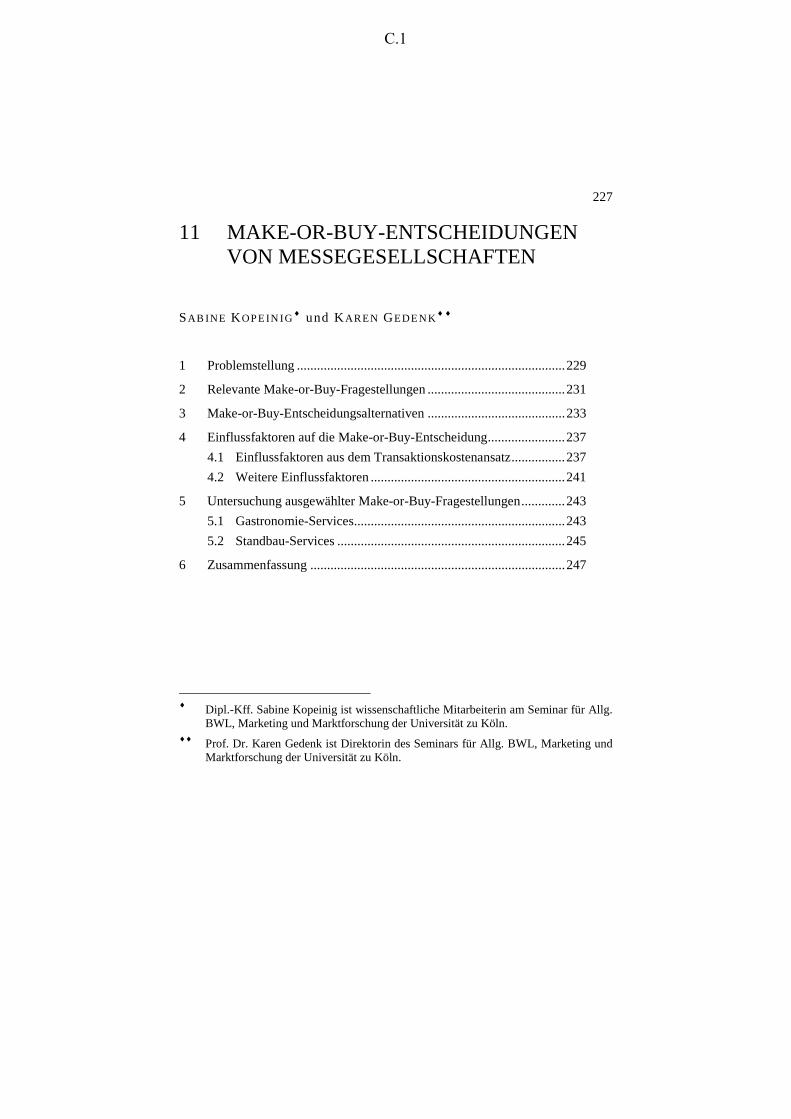
227
11 MAKE-OR-BUY-ENTSCHEIDUNGEN VON MESSEGESELLSCHAFTEN
SAB INE KOP E IN IG♦ und KAREN GEDE N K
♦ ♦
1 Problemstellung ................................................................................229
2 Relevante Make-or-Buy-Fragestellungen .........................................231
3 Make-or-Buy-Entscheidungsalternativen .........................................233
4 Einflussfaktoren auf die Make-or-Buy-Entscheidung.......................237
4.1 Einflussfaktoren aus dem Transaktionskostenansatz................237 4.2 Weitere Einflussfaktoren ..........................................................241
5 Untersuchung ausgewählter Make-or-Buy-Fragestellungen.............243
5.1 Gastronomie-Services...............................................................243 5.2 Standbau-Services ....................................................................245
6 Zusammenfassung ............................................................................247
♦ Dipl.-Kff. Sabine Kopeinig ist wissenschaftliche Mitarbeiterin am Seminar für Allg.
BWL, Marketing und Marktforschung der Universität zu Köln. ♦♦ Prof. Dr. Karen Gedenk ist Direktorin des Seminars für Allg. BWL, Marketing und
Marktforschung der Universität zu Köln.
C.1

C.2

M A K E - O R - B U Y - E N T S C H E I D U N G E N
229
1 Problemstellung
Unter einer Make-or-Buy-Entscheidung wird die Entscheidung zwischen dem Fremdbezug oder der Eigenfertigung von Leistungen verstanden. Die „Make“-Entscheidung entspricht dabei der Eigenfertigung bzw. der vertikalen Integra-tion, während man unter „Buy“ den Bezug am Markt bzw. ein Outsourcing versteht. Zwischen diesen beiden Extremen gibt es eine Vielzahl relevanter Ko-operationsformen als Hybride.1
Messegesellschaften sehen sich an vielen Stellen mit Make-or-Buy-Entscheidungen konfrontiert, z.B. bei der Datenverarbeitung und beim Aus-landsvertrieb. Besonders relevant ist die Frage nach „Make or Buy“ derzeit in vielen Messegesellschaften bei den Services, welche sie Ausstellern und Messe-besuchern anbieten. Dazu zählen beispielsweise Gastronomie-, Standbau-, Logistik- und Reise-Services. Deutsche Messegesellschaften konkurrieren heute nicht nur untereinander, sondern stehen auch mit nationalen privaten Messever-anstaltern im Wettbewerb.2 Darüber hinaus verschärft sich der internationale Wettbewerb um den Messeplatz Deutschland. Des Weiteren müssen deutsche Messegesellschaften gestiegene Kundenwünsche sowohl seitens der Messeaus-steller als auch der –besucher erfüllen. Um sich in diesem Umfeld abheben zu können, setzen deutsche Messegesellschaften verstärkt darauf, ihren Kunden ein „Full-Service-Paket“ zu schnüren. Das Ziel dabei ist es insbesondere, den Aus-stellern sämtliche Dienstleistungen im Rahmen der Messebeteiligung aus einer Hand anzubieten („one face to the customer“). Hier ergibt sich z.T. ein erhebli-ches Erlös- bzw. Gewinnpotenzial.3 Die entsprechenden Leistungen müssen aber nicht notwendigerweise selbst erstellt werden. Für Messegesellschaften ist es daher wichtig, sich mit Make-or-Buy-Entscheidungen für ergänzende Services auseinander zu setzen.
Make-or-Buy-Fragestellungen sind Gegenstand zahlreicher wissenschaftlicher und nicht-wissenschaftlicher Publikationen.4 Dabei werden insbesondere Be-schaffungsprozesse produzierender Unternehmen betrachtet, aber auch andere
1 Vgl. Picot (1991), S. 339; Williamson (1991), S. 269. 2 Vgl. Witt (2003), S. 506. 3 Vgl. AUMA-Bericht (2001/2002), S. 5; Die Welt (2005), S. 13. 4 Vgl. z.B. Walker / Weber (1984) oder Liebermann (1991). Einen ausführlichen
Literaturüberblick über empirische Studien gibt Klein (2004).
C.3

K O P E I N I G ⋅ G E D E N K
230
betriebliche Teilfunktionen wie die Datenverarbeitung oder der Vertrieb. Bei-spielsweise kann die Frage, ob der Vertrieb über einen unternehmenseigenen Außendienst oder über rechtlich selbständige Personen bzw. Unternehmen durchgeführt werden soll, als eben solche Entscheidung aufgefasst werden.5 ZYGOJANNIS diskutiert diese Fragestellung im Beitrag: „Gestaltung des Aus-landsvertriebs“. Im Fokus der Literatur zu „Make or Buy“ steht die Identifikation von Einflussfaktoren, welche eine „Make“- oder aber eine „Buy“-Entscheidung vorteilhafter erscheinen lassen. Solche Einflussfaktoren lassen sich zunächst aus dem Transaktionskostenansatz ableiten. Diese auf COASE zurückgehende und v.a. durch WILLIAMSON weiterentwickelte Theorie identifiziert zentrale Einfluss-faktoren wie Spezifität und Komplexität der zu erbringenden Leistung, anhand derer eine Überprüfung der Vorteilhaftigkeit verschiedener Entscheidungsalter-nativen möglich ist.6 Darüber hinaus zeigt die konzeptionelle Literatur zu den jeweils betrachteten Entscheidungen weitere Einflussfaktoren auf.
Make-or-Buy-Entscheidungen im Messewesen sind in der Literatur bislang nicht thematisiert worden. Die Übertragung von Erkenntnissen der bisherigen Literatur zu Make-or-Buy-Entscheidungen ist nicht ohne weiteres möglich. Zum einen sind die Einflussfaktoren des Transaktionskostenansatzes sehr abstrakt und bedürfen einer Konkretisierung und Anwendung auf den Messe-Kontext. Zum anderen ist die konzeptionelle Literatur zum Messewesen bislang nicht systema-tisch unter dem Gesichtspunkt von Make-or-Buy-Entscheidungen ausgewertet worden. So ergeben sich bei Messen Besonderheiten im Vergleich zu anderen Branchen z.B. aus der Existenz von Mehrfachzielen der Anteilseigner (Gewinn und Umwegrendite).
Ziel unseres Beitrags ist es daher, einen Überblick über Make-or-Buy-Entscheidungen von Messegesellschaften zu geben. Wir wollen relevante Ent-scheidungen und Entscheidungsalternativen identifizieren und Einflussfaktoren auf die Vorteilhaftigkeit der Handlungsalternativen diskutieren. Der Beitrag beginnt in Abschnitt 2 mit einer Systematisierung von Make-or-Buy-Entscheidungen von Messegesellschaften. Abschnitt 3 zeigt auf, welche Ent-scheidungsalternativen dabei zur Verfügung stehen. Beispiele machen deutlich, dass Messegesellschaften durchaus zu unterschiedlichen Entscheidungen gelan-gen, was noch einmal die Bedeutung der Fragestellung unterstreicht. In Abschnitt 4 präsentieren wir Einflussfaktoren auf die Vorteilhaftigkeit von „Make“ vs. „Buy“, die wir zum einen aus dem Transaktionskostenansatz ableiten (Abschnitt 4.1) und zum anderen aus der konzeptionellen Literatur zum Messe-
5 Vgl. z.B. Anderson (1985) oder Krafft / Albers / Lal (2004). 6 Vgl. Coase (1937); Williamson (1975); Williamson (1985).
C.4

M A K E - O R - B U Y - E N T S C H E I D U N G E N
231
wesen (Abschnitt 4.2). Diese Einflussfaktoren werden anschließend in Abschnitt 5 eingesetzt, um exemplarisch die Vorteilhaftigkeit von Eigenfertigung vs. Fremdbezug bei Gastronomie- und Standbau-Services zu prüfen. Der Beitrag schließt mit einer Zusammenfassung in Abschnitt 6.
2 Relevante Make-or-Buy-Fragestellungen
Im Folgenden betrachten wir Messegesellschaften als Veranstalter von Messen mit eigenem Gelände und überwiegend eigenem Messeprogramm. In Deutsch-land befinden sich diese Messegesellschaften zumeist im Besitz von Kommunen und/oder Bundesländern. Damit erfolgt eine Abgrenzung von reinen Betriebsge-sellschaften, die hier nicht betrachtet werden sollen.7
Die Analyse von Make-or-Buy-Entscheidungen ist grundsätzlich für viele Funk-tionsbereiche und Aktivitäten von Messegesellschaften relevant. Abbildung 13 gibt einen Überblick über diese Aktivitäten in Form einer Wertschöpfungskette.
So denken Messegesellschaften zum einen darüber nach, sekundäre Aktivitäten wie die Datenverarbeitung oder die Lohn- und Gehaltsverrechnung aus dem Unternehmen auszulagern. Diese Entscheidungen zu sekundären Aktivitäten werden hier nicht weiter betrachtet, da sie nicht messespezifisch sind.
Zum anderen können primäre Aktivitäten der Gegenstand von Make-or-Buy-Überlegungen sein. Die zentrale, primäre Aktivität einer Messegesellschaft besteht in der räumlichen und zeitpunktbezogenen Zusammenführung von Besu-chern und Ausstellern, typischerweise von (potenziellen) Käufern und Verkäu-fern, in einem Markt.8 Das Kerngeschäft der Messegesellschaft ist dabei die Präsentation von Branchen, Firmen und Produkten.9 Hier stellt sich die Make-or-Buy-Fragestellung kaum, da Aktivitäten des Kerngeschäfts von hoher strategi-scher Bedeutung sind und in aller Regel im Unternehmen bleiben.10
7 Vgl. Groth (1992), S. 161. 8 Vgl. Stoeck (1999), S. 29f. 9 Vgl. Goschmann (2003), S. 46. 10 Vgl. Quinn (1999), S. 43.
C.5
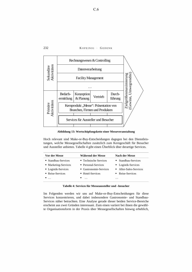
K O P E I N I G ⋅ G E D E N K
232
Rechnungswesen & Controlling
Datenverarbeitung
FacilityManagement
…
Seku
ndär
e A
ktiv
ität
enP
rim
äre
Akt
ivit
äten
Bedarfs-ermittlung
Konzeption& Planung Vertrieb
Durch-führung
Kernprodukt „Messe“: Präsentation von Branchen, Firmen und Produkten
Services für Aussteller und Besucher
Zie
lgrö
ßenm
axim
ieru
ng(G
ewin
n, U
mw
egre
ndit
e)
Abbildung 13: Wertschöpfungskette einer Messeveranstaltung
Hoch relevant sind Make-or-Buy-Entscheidungen dagegen bei den Dienstleis-tungen, welche Messegesellschaften zusätzlich zum Kerngeschäft für Besucher und Aussteller anbieten. Tabelle 4 gibt einen Überblick über derartige Services.
Vor der Messe Während der Messe Nach der Messe
Standbau-Services
Marketing-Services
Logistik-Services
Reise-Services
…
Technische Services
Personal-Services
Gastronomie-Services
Hotel-Services
…
Standbau-Services
Logistik-Services
After-Sales-Services
Reise-Services
…
Tabelle 4: Services für Messeaussteller und –besucher
Im Folgenden werden wir uns auf Make-or-Buy-Entscheidungen für diese Services konzentrieren, und dabei insbesondere Gastronomie- und Standbau-Services näher betrachten. Eine Analyse gerade dieser beiden Service-Bereiche erscheint aus zwei Gründen interessant. Zum einen variiert bei ihnen die gewähl-te Organisationsform in der Praxis über Messegesellschaften hinweg erheblich,
C.6

M A K E - O R - B U Y - E N T S C H E I D U N G E N
233
wie im folgenden Abschnitt gezeigt wird. Zum anderen wird so eine Dienstleis-tung betrachtet, die sich primär an die Aussteller richtet (Standbau), und eine weitere, deren Zielgruppe vor allem Besucher sind (Gastronomie).
Gastronomie-Services stellen aufgrund hoher und unterschiedlicher Erwartungen der Messekunden einen bedeutenden und gleichzeitig problematischen Service-bereich dar.11 Messeaussteller und –besucher erwarten eine umfassende, qualita-tiv hochwertige und preisgünstige gastronomische Versorgung auf dem Messe-gelände. Diese umfasst neben dem Betrieb unterschiedlicher Restaurants, Bistros und Snack-Points auch die Standbelieferung sowie das Veranstaltungscatering, z.B. bei Pressekonferenzen oder Empfängen.
Zu den Standbau-Services zählen die Planung, Konzeption und Umsetzung sowie Montage und Demontage des Messestandes. Ausgaben für den Messestand stellen einen großen Kostenblock für Aussteller und somit ein erhebliches Um-satzpotenzial für Messegesellschaften dar. Messestandbauer arbeiten im Auftrag der Messegesellschaften und/oder der Messeaussteller. Ersteres ist insbesondere dann der Fall, wenn Messegesellschaften Mietnormstände anbieten.
3 Make-or-Buy-Entscheidungsalternativen
Make-or-Buy-Entscheidungen sollen hier nicht als Entweder-Oder-Entscheidungen begriffen werden. Vielmehr gibt es zwischen den Alternativen Eigenerstellung („Make“) und Einkauf am Markt („Buy“) eine Vielzahl relevan-ter Mischformen, bei denen Messegesellschaften mit anderen Unternehmen ko-operieren („Cooperate“). In Abbildung 14 sind mögliche Entscheidungsalternati-ven dargestellt. Der Grad der vertikalen Integration nimmt dabei von oben nach unten ab.
11 Vgl. Tauberger / Wartenberg (1992), S. 240.
C.7

K O P E I N I G ⋅ G E D E N K
234
Eigenentwicklung und Eigenerstellung
Kapitalbeteiligung an Messedienstleistern
Ansiedlung von Messedienstleistern auf demMessegelände
Entwicklungskooperation mit anschließenderEigenerstellung oder Fremdbezug
Langzeitvereinbarungen mit Messedienstleistern
Jahresverträge mit offenen (fixierten) Liefer-terminen und Liefermengen, Kontingente
(spontaner) Einkauf am Markt
Grad dervertikalen
Integration
Make
Buy
Cooperate
Abbildung 14: Make-or-Buy-Entscheidungsalternativen12
Messegesellschaften wählen durchaus unterschiedliche Grade der vertikalen Integration bei den verschiedenen Dienstleistungen. Beispielhaft sei hier die Koelnmesse Service GmbH angeführt, die im Bereich der ergänzenden Dienst-leistungen nahezu das komplette Spektrum möglicher Entscheidungsalternativen abdeckt. So bietet die Koelnmesse Service GmbH technische Services aus eigener Hand an. Im Bereich der Standbau-Services unterhält sie eine Kooperati-onsvereinbarung mit dem Partnerunternehmen Uniplan. Darüber hinaus bestehen langfristige Vertragsbeziehungen mit Dienstleistern, z.B. Pachtverträge mit Messegastronomen. Dabei wird zumeist mittelständischen, ortsansässigen Unter-nehmen das Recht eingeräumt, gastronomische Anlagen auf dem Messegelände (in Messehallen) zu nutzen und gewinnbringend zu betreiben. Einige Dienst-leistungen, wie z.B. Personal-Services (Standpersonal, Standbewachung) oder Hotel-Services (Partnerhotels) werden lediglich zwischen Messeausstellern und Drittunternehmen vermittelt.
Andere deutsche Messegesellschaften haben im Bereich ergänzender Dienstleis-tungen andere Strukturen vorgezogen. Beispielsweise werden Gastronomie-Services von der Messe Frankfurt ausschließlich über ein eigenes Tochterunter-nehmen angeboten (Accente Gastronomie Service GmbH). Auch die Leipziger Messe verfügt über ein Tochterunternehmen im Gastronomiebereich. Ob auch messefremde Unternehmen durch Messeaussteller etwa für das Standcatering
12 In Anlehnung an Picot (1991), S. 340.
C.8

M A K E - O R - B U Y - E N T S C H E I D U N G E N
235
beauftragt werden dürfen, hängt von der Unternehmenspolitik der einzelnen Messegesellschaften ab. Auf dem Messegelände Frankfurt dürfen Messeausstel-ler Fremdcaterer nur nach Absprache mit Accente (gegen eine Ausfallentschädi-gung) beauftragen. Auf den Messegeländen Hannover, München, Leipzig u.a. ist die Standbewirtung dagegen offen und kann auch von messefremden Unter-nehmen betreut werden.13
Im Servicebereich Standbau betreibt die Leipziger Messe eine vollständige Integration in der Form, dass Standbau-Services über ein Tochterunternehmen mit unternehmenseigenem Personal angeboten werden. Eine hybride Organisati-onsform hat hier die Messe München gewählt, die zu 85% an der Messe-planungs- und Messebaufirma Meplan beteiligt ist. Ein weiteres Beispiel für eine vertikale Kooperation findet sich bei der Nürnberg Messe GmbH. Sie bietet zusammen mit drei Messebauunternehmen über das Internetportal www.standkonfigurator.de elf unterschiedliche Standbaumodelle an, welche gemeinsam entwickelt wurden.
Tabelle 5 zeigt diese und andere Praxisbeispiele noch einmal im Überblick.
13 Vgl. m+a report, (2003), S. 48f.
C.9

K O P E I N I G ⋅ G E D E N K
236
Services Entscheidungs-
alternative Gastronomie Standbau Weitere
Eigenerstellung (Make)
Frankfurt: Tochter-unternehmen Ac-cente Gastronomie Service GmbH
Leipzig: Tochter-unternehmen Leip-ziger Messe Gastro-nomie GmbH
Leipzig: Tochter-unternehmen FAIRNET – Gesellschaft für Messe-, Ausstel-lungs- und Veranstaltungs-service mbH
Technische Servi-ces, Köln: Angebot von Elektroinstal-lationen aus eigener Hand
Kapitalbeteili-gung an Messe-dienstleistern
München: 85 % Kapitalbeteiligung an der Messe-baufirma Meplan GmbH
Ansiedlung von Messe-dienstleistern
Logistik, Stuttgart: Speditionsunter-nehmen Schenker unterhält auf dem Messegelände ganz-jährig ein Büro
Entwicklungs-kooperation
Nürnberg: Koope-ration mit drei Messebauern
Langzeitverein-barungen mit Messedienst-leistern
Köln: Pachtvertrag mit einem Messe-gastronom
München: Pacht-verträge mit zwei Messegastronomen
Köln: Kooperati-on mit Uniplan
Kontingent-vereinbarungen
Hotel, Köln: Kontingentverein-barungen mit Part-nerhotels im Raum Köln
Tabelle 5: Praxisbeispiele – Entscheidungsalternativen
C.10

M A K E - O R - B U Y - E N T S C H E I D U N G E N
237
Es kann also festgehalten werden, dass Make-or-Buy-Entscheidungen nicht nur über Services variieren, sondern auch bei der gleichen Dienstleistung über Messegesellschaften hinweg. Dies macht es umso interessanter, im Folgenden Einflüsse auf die Vorteilhaftigkeit der verschiedenen Entscheidungsalternativen zu diskutieren.
4 Einflussfaktoren auf die Make-or-Buy-Entscheidung
4.1 Einflussfaktoren aus dem Transaktionskostenansatz
Der Transaktionskostenansatz geht auf COASE zurück und ist vor allem von WILLIAMSON entscheidend weiterentwickelt worden.14 Der Fokus der Theorie liegt auf den Austauschbeziehungen bzw. Transaktionen zwischen Unterneh-men.15 Unter einer Transaktion wird dabei die Übertragung von Verfügungsrech-ten an Gütern und Dienstleistungen zwischen Wirtschaftssubjekten verstanden.16 WILLIAMSON hält fest, dass jedes Problem, das direkt oder indirekt als Vertrags-problem zu formulieren ist, mit Hilfe der Transaktionskostentheorie untersucht werden kann.17
Transaktionen können entweder innerhalb der Unternehmensgrenzen bzw. in Hierarchien („Make“) oder aber am Markt („Buy“) durchgeführt werden. Unter-nehmen sollten dabei diejenige Transaktionsform wählen, welche die niedrigeren Transaktionskosten aufweist.18 Unter Transaktionskosten werden in diesem Zu-sammenhang die Kosten der Anbahnung, Vereinbarung, Abwicklung, Kontrolle und Anpassung der mit den einzelnen Phasen einer Transaktion verbundenen Aktivitäten verstanden.19 Höhe und Struktur der Transaktionskosten für die einzelnen Handlungsalternativen hängen von den Eigenschaften der jeweiligen Leistung (Transaktionsdimensionen) ab.20 WILLIAMSONS mikroanalytischer Ana-
14 Vgl. Coase (1937); Williamson (1975); Williamson (1985). 15 Vgl. Rindfleisch / Heide (1997), S. 30. 16 Vgl. Williamson (1990), S. 20. 17 Vgl. Williamson (1990). 18 Vgl. Bogaschewsky (1995), S. 164. 19 Vgl. Picot (1991), S. 344; Picot (1982), S. 270. 20 Vgl. Picot (1991), S. 344.
C.11

K O P E I N I G ⋅ G E D E N K
238
lyserahmen beruht im Wesentlichen auf dem Wechselspiel zwischen Annahmen über das menschliche Verhalten und diesen Transaktionsdimensionen. Mit den zentralen Verhaltensannahmen der begrenzten Rationalität und des Opportunis-mus wird die neoklassische Annahme des „homo oeconomicus“ aufgegeben.21
Darüber hinaus trifft WILLIAMSON die Annahme der Risikoneutralität. Zu den Transaktionsdimensionen zählen Spezifität, Unsicherheit/Komplexität und Häu-figkeit.22 Abbildung 15 zeigt die geschilderten Zusammenhänge noch einmal im Überblick.
TransaktionskostenKosten für die Anbahnung, Vereinbarung,
Abwicklung, Kontrolle und Anpassungvon Transaktionen
Eigenschaften derTransaktionspartnerVerhaltensannahmen:- beschränkte Rationalität- Opportunismus- Risikoneutralität
Eigenschaften von Leistung und Umwelt- Spezifität- Unsicherheit/Komplexität- Häufigkeit
Wahl einer Handlungsalternative- Make- Cooperate- Buy
Abbildung 15: Grundgedanke des Transaktionskostenansatzes
Die Eigenschaften der Leistung bzw. der Umwelt stellen wesentliche Einflüsse auf die Vorteilhaftigkeit der Make-or-Buy-Handlungsalternativen dar. Unter Spezifität versteht man die exklusive Gestaltung und Widmung von Ressour-
21 Vgl. Williamson (1990), S. 34. 22 Vgl. Williamson (1990), S. 59ff.; Williamson (1991), S. 281.
C.12

M A K E - O R - B U Y - E N T S C H E I D U N G E N
239
cen.23 Wenn zur Erstellung einer Leistung bestimmte Ressourcen notwendig sind, die nur unter großen Verlusten anders beschafft werden könnten, spricht man von hoher Spezifität. Beispielhafte Ressourcen sind Werkzeuge oder Maschinen. Aber auch Know-how, Personalqualifikation oder Qualitätseigen-schaften können spezifisch sein. Im Einzelnen unterscheidet WILLIAMSON (1991) zwischen sechs Formen der Spezifität, welche in Tabelle 6 wiedergegeben sind.24
Form Investitionen der Transaktionspartner …
Standort-Spezifität
in ortsgebundene Einrichtungen
Sachkapital-Spezifität
in spezifische Maschinen oder Technologien
Humankapital-Spezifität
in spezifische Mitarbeiterqualifikation
Marken-Spezifität
in den Markennamen
Widmungs-Spezifität
in nichtspezifische Anlagen, die aber nur für die geplante Transaktion erfolgen und bei deren Wegfall Überkapazitäten entste-hen
Temporäre Spezifität
müssen in einem engen, zeitlichen Rahmen getätigt werden (z.B. Montagearbeiten, Just-in-time-Produktion)
Tabelle 6: Formen der Spezifität
Eine Kernaussage des Transaktionskostenansatzes ist, dass hohe Spezifität zum Versagen von Marktmechanismen führt.25 Bei einer „Buy“-Lösung würden sich beide Marktpartner in eine starke wechselseitige Abhängigkeit begeben. Dies kann nur bei gegenseitigem Vertrauen erfolgreich sein. Liegt dagegen opportu-nistisches Verhalten vor, muss jeder Vertragspartner befürchten, dass sein Ge-genüber den Vertrag auflöst und spezifische Investitionen verloren gehen. Eine hohe Spezifität von Transaktionen spricht daher für eine hierarchische, d.h. für eine „Make“-Lösung.
Die zweite Transaktionsdimension ist Unsicherheit/Komplexität. Unsicherheit bezieht sich auf qualitative, quantitative, terminliche oder technische Änderun-
23 Vgl. Picot (1991), S. 347. 24 Vgl. Williamson (1991), S. 281. 25 Vgl. Picot / Dietl (1990), S. 180.
C.13

K O P E I N I G ⋅ G E D E N K
240
gen der im Fokus der Untersuchung stehenden Leistung bzw. der Unternehmens-umwelt. Im Falle von Komplexität sind Leistung und Umwelt zwar sicher, aufgrund begrenzter Rationalität aber nicht vollständig überschaubar.26 Hohe Unsicherheit bzw. Komplexität sprechen dafür, Transaktionen nicht rein über Märkte durchzuführen, sondern stärker vertraglich abzusichern. Dies gilt insbe-sondere bei hoher Spezifität, da in diesem Fall nicht einfach am Markt neue Tauschbeziehungen eingegangen werden können.27
Eine weitere Transaktionsdimension ist die Häufigkeit der Durchführung. Wird eine Leistung häufig und regelmäßig benötigt, so dürfte aufgrund von Skalen- und Lerneffekten eine Eigenerstellung besonders vorteilhaft sein. Dies gilt insbe-sondere bei hoher Spezifität. Eine hoch spezifische Leistung wird im Extremfall von einem Zulieferer nur für einen Abnehmer erbracht. Damit hat der Zulieferer in Bezug auf diese hochspezifische Transaktion keine Skalenvorteile gegenüber dem Abnehmer, falls dieser die nachgefragte Leistung selbst erstellt.28
Tabelle 7 fasst die Hypothesen des Transaktionskostenansatzes zu Einflüssen auf die Make-or-Buy-Entscheidung noch einmal zusammen. Man erkennt, dass eine hierarchische im Vergleich zu einer Marktlösung umso vorteilhafter ist, je höher Spezifität, Unsicherheit/Komplexität und Häufigkeit sind.
Einflussfaktor Vorteilhaftigkeit von „Make“ vs. „Buy“
Spezifität +
Unsicherheit/Komplexität +
Häufigkeit +
Tabelle 7: Hypothesen zu Einflussfaktoren des Transaktionskostenansatzes
26 Vgl. Picot/Dietl (1990), S. 179. 27 Vgl. Klein (2004), S. 14. 28 Vgl. Bogaschewsky (1995), S. 168 f.
C.14

M A K E - O R - B U Y - E N T S C H E I D U N G E N
241
4.2 Weitere Einflussfaktoren
Neben den transaktionskostenbezogenen Faktoren sind auch ziel-, ressourcen- und marktbezogene Einflussfaktoren zu berücksichtigen, die sich aus der kon-zeptionellen Marketing- und Messeliteratur ableiten lassen. Tabelle 8 gibt einen Überblick über relevante Faktoren und die entsprechenden Hypothesen.
Tabelle 8: Weitere Einflussfaktoren
Zu den zielbezogenen Einflussfaktoren zählt zunächst die Bedeutung der Leistung für das Unternehmen.29 Wie bereits in Abschnitt 2 diskutiert, werden Kernaktivitäten von besonderer strategischer Relevanz sicherlich im Unterneh-men durchgeführt werden. Aber auch für andere Transaktionen gilt, dass die Organisationsform umso stärker zu einem „Make“ tendieren sollte, je größer die Bedeutung der Leistung für das Unternehmen ist.
Des Weiteren sind die besonderen Besitzverhältnisse von Messegesellschaften zu beachten, die dazu führen können, dass Anteilseigner mehrere Ziele verfolgen. So streben Kommunen bzw. Länder als typische Mehrheitseigner von Messe-
29 Vgl. Picot (1991), S. 346.
Einflussfaktor Vorteilhaftigkeit von „Make“ vs. „Buy“
Zielbezogene Einflussfaktoren
Bedeutung der Leistung +
Ziele Umwegrendite − / +
Ressourcenbezogene Einflussfaktoren
Know-how-Bedarf −
Kapitalbedarf −
Technologie-Bedarf −
Marktbezogene Einflussfaktoren
Bedeutung von Kundennähe +
Qualitätsanforderungen +
+ positiver Einfluss − negativer Einfluss
C.15

K O P E I N I G ⋅ G E D E N K
242
gesellschaften in Deutschland in der Regel nicht nur einen hohen Gewinn der Messen an, sondern verfolgen auch gesellschafts- und regionalpolitische Ziele.30 Vielfach wird hier die Umwegrendite als Erfolgsgröße herangezogen, welche widerspiegelt, welchen Einfluss Messen auf das wirtschaftliche Umfeld haben, z.B. im Hotel- und Gastronomiebereich. Die Koelnmesse beispielsweise beziffert die Umwegrendite für 2003 mit 4,90 Euro. Dies bedeutet, dass jeder durch die Koelnmesse erzielter Euro Umsatz den im Raum Köln ansässigen Unternehmen Umsätze in Höhe von 4,90 Euro bescherte. Öffentliche Institutionen als Anteils-eigner haben somit ein Interesse daran, dass Transaktionen von in der Region an-sässigen Unternehmen durchgeführt werden. Dies könnte Entscheidungen zur vertikalen Integration erschweren, wenn die Befürchtung besteht, der regionalen Wirtschaft Geschäft zu entziehen. In erster Linie sprechen die Ziele der Anteils-eigner jedoch für eine vertikale Integration, wenn anderenfalls außerhalb der Re-gion ansässige Unternehmen die Leistung erstellen würden.
In Zusammenhang mit ressourcenbezogenen Einflussfaktoren muss eine Messe-gesellschaft prüfen, ob die Dienstleistung besondere Anforderungen in Bezug auf das erforderliche Know-how sowie die notwendige Technologie und Kapitalaus-stattung stellt. Eine Integration von Services, die sich im Hinblick auf die Struk-tur, die Technologie und das Management wesentlich vom Kerngeschäft unter-scheiden, ist oftmals mit prohibitiven Transaktionskosten verbunden.31
Schließlich muss die Messegesellschaft auch marktbezogene Einflussfaktoren berücksichtigen.32 Durch die Eigenerstellung von Dienstleistungen agiert die Messegesellschaft sehr marktnah und erhält quasi aus erster Hand Kundeninfor-mationen, z.B. Kenntnisse über die Präferenzen von Messeausstellern und –besuchern. Diese Informationen kann die Messegesellschaft im Wettbewerb für sich nutzen. Eine hohe Bedeutung von Marktnähe und den entsprechenden Kundeninformationen spricht daher für die vertikale Integration. Auch hohe Qualitätsanforderungen sprechen tendenziell dafür, Leistungen selbst zu erstel-len, da hier eine stärkere Kontrolle gewährleistet werden kann.
30 Vgl. Groth (1992), S. 162. 31 Vgl. Picot (1991), S. 347f. 32 Vgl. Homburg / Krohmer (2003), S. 711ff. Die Autoren fassen diese Einfluss-
faktoren als „Effektivitätsüberlegungen“ zusammen.
C.16

M A K E - O R - B U Y - E N T S C H E I D U N G E N
243
5 Untersuchung ausgewählter Make-or-Buy-Fragestellungen
Nachdem mögliche Make-or-Buy-Fragestellungen im Bereich der Services für Messeaussteller und –besucher identifiziert, Entscheidungsalternativen auf-gezeigt und Einflussfaktoren benannt wurden, soll nun exemplarisch für Gastro-nomie- und Standbau-Services eine Make-or-Buy-Analyse durchgeführt werden. Dazu werden die in Abschnitt 4 diskutierten Einflussfaktoren auf die Vorteilhaf-tigkeit von „Make“- vs. „Buy“-Entscheidungen herangezogen.
5.1 Gastronomie-Services
Bei den Gastronomie-Services ist zunächst die Spezifität als sehr hoch einzu-stufen. Hier sind hohe Investitionen in standort- und sachkapitalspezifische Ein-richtungen erforderlich. Insbesondere müssen Ausstattungsinvestitionen, z.B. für Großküchen- oder Restaurantausstattungen, getätigt werden, die bei Abbruch der Transaktion nicht anderweitig eingesetzt werden können. Unsicherheit und Komplexität sind für Gastronomie-Services eher als gering einzustufen. Die Nachfrage ist vergleichsweise einfach zu prognostizieren, und größere Marktver-änderungen sind wenig wahrscheinlich. Schließlich kann die Häufigkeit der Transaktionen als groß bezeichnet werden, da Gastronomie-Services auf jeder Messe angeboten werden.
Bei den zielbezogenen Einflussfaktoren ist die Bedeutung von Gastronomie-Services für Messegesellschaften tendenziell gering bis mittel. Zwar kann eine schlechte Dienstleistungsqualität zu erheblicher Verärgerung bei Messeausstel-lern und –besuchern führen, und ein qualitativ hochwertiges Angebot kann ein gewisses Differenzierungspotential gegenüber den Wettbewerbern bieten.33 Zentral für die Entscheidung von Ausstellern und Besuchern, an einer Messe teilzunehmen, dürften jedoch eher andere Faktoren sein. Vorgaben von Anteils-eignern in Zusammenhang mit dem Ziel der Umwegrendite sind bei Gastrono-mie-Services nicht zu erwarten, da davon auszugehen ist, dass sowohl bei einer markt- als auch einer hierarchienahen Lösung die Wertschöpfung in der Messe-region verbleibt.
33 Vgl. Suhling (2003), S. 1123.
C.17
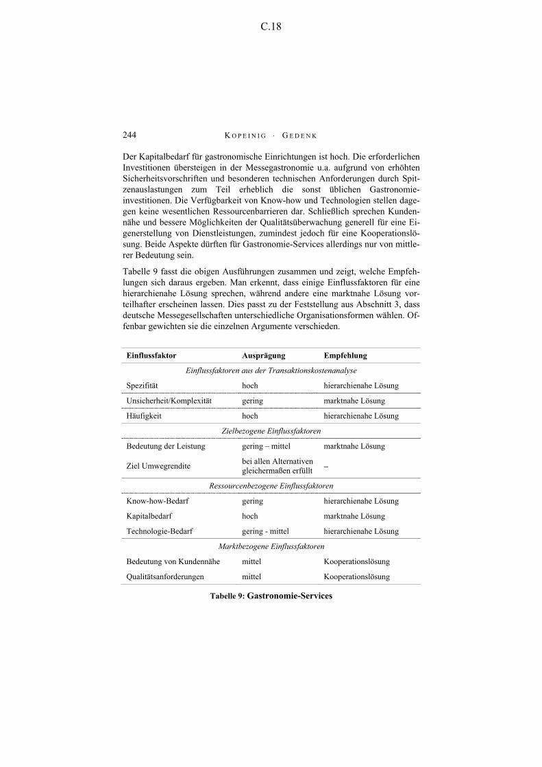
K O P E I N I G ⋅ G E D E N K
244
Der Kapitalbedarf für gastronomische Einrichtungen ist hoch. Die erforderlichen Investitionen übersteigen in der Messegastronomie u.a. aufgrund von erhöhten Sicherheitsvorschriften und besonderen technischen Anforderungen durch Spit-zenauslastungen zum Teil erheblich die sonst üblichen Gastronomie-investitionen. Die Verfügbarkeit von Know-how und Technologien stellen dage-gen keine wesentlichen Ressourcenbarrieren dar. Schließlich sprechen Kunden-nähe und bessere Möglichkeiten der Qualitätsüberwachung generell für eine Ei-generstellung von Dienstleistungen, zumindest jedoch für eine Kooperationslö-sung. Beide Aspekte dürften für Gastronomie-Services allerdings nur von mittle-rer Bedeutung sein.
Tabelle 9 fasst die obigen Ausführungen zusammen und zeigt, welche Empfeh-lungen sich daraus ergeben. Man erkennt, dass einige Einflussfaktoren für eine hierarchienahe Lösung sprechen, während andere eine marktnahe Lösung vor-teilhafter erscheinen lassen. Dies passt zu der Feststellung aus Abschnitt 3, dass deutsche Messegesellschaften unterschiedliche Organisationsformen wählen. Of-fenbar gewichten sie die einzelnen Argumente verschieden.
Einflussfaktor Ausprägung Empfehlung
Einflussfaktoren aus der Transaktionskostenanalyse
Spezifität hoch hierarchienahe Lösung
Unsicherheit/Komplexität gering marktnahe Lösung
Häufigkeit hoch hierarchienahe Lösung
Zielbezogene Einflussfaktoren
Bedeutung der Leistung gering – mittel marktnahe Lösung
Ziel Umwegrendite bei allen Alternativen gleichermaßen erfüllt −
Ressourcenbezogene Einflussfaktoren
Know-how-Bedarf gering hierarchienahe Lösung
Kapitalbedarf hoch marktnahe Lösung
Technologie-Bedarf gering - mittel hierarchienahe Lösung
Marktbezogene Einflussfaktoren
Bedeutung von Kundennähe mittel Kooperationslösung
Qualitätsanforderungen mittel Kooperationslösung
Tabelle 9: Gastronomie-Services
C.18

M A K E - O R - B U Y - E N T S C H E I D U N G E N
245
5.2 Standbau-Services
Die Spezifität von Standbau-Services ist als eher gering einzustufen. Standort- und sachkapitalspezifische Investitionen fallen nur in geringem Maße an, da die meisten Einrichtungen und Maschinen häufig auch bei Beziehungsabbruch weiterhin zum Einsatz kommen können. Auch die Unsicherheit in Bezug auf Leistungen und Umwelt ist eher gering. Schließlich ist die Häufigkeit der Trans-aktionen hoch. Die daraus folgenden Kostendegressions-Effekte sind dann besonders groß, wenn Standbau-Services auch für andere Messeplätze angeboten werden können.
Ähnlich wie bei den Gastronomie-Services sind auch Standbau-Services von geringer bis mittlerer strategischer Bedeutung für Messegesellschaften. Ein ge-lungener Standbau ist zwar wichtig für Messeaussteller. Aufgrund der Existenz zahlreicher Standbau-Unternehmen mit qualitativ hochwertigem Angebot ist das Differenzierungspotenzial für Anbieter allerdings begrenzt. Die Zielsetzung Umwegrendite könnte bei Standbau-Services tendenziell dazu führen, dass eine hierarchienahe Lösung bevorzugt wird. Ist bei einer Markt-Lösung doch zu be-fürchten, dass Standbau-Aufträge in erheblichem Umfang an nicht ortsansässige Unternehmen vergeben werden.
Bezüglich der Ressourcen geht eine Eigenerstellung der Standbauaktivitäten mit der Bereitstellung von erheblicher maschineller Ausrüstung und personellem Know-how einher. Auch wenn die erforderlichen Technologien bereit stehen, ist der Kapitalbedarf auf jeden Fall groß.
Schließlich kann die Bedeutung der Kundennähe in Bezug auf den Standbau als mittel eingestuft werden. Die Qualität von Messeständen muss aus Aussteller-sicht sehr gut sein. Der Messestand ist der Kulminationspunkt eines ausstellen-den Unternehmens und repräsentiert für die Tage der Veranstaltung den Unter-nehmenssitz.34 Um die Qualität sicherzustellen und zu kontrollieren, könnte man eine hierarchienahe Lösung empfehlen. Allerdings sind in Deutschland Messe-bauunternehmen im FAMAB35 organisiert. Um in diesem aufgenommen zu wer-den, müssen hohe Qualitätskriterien erfüllt und eingehalten werden. Im Bereich
34 Vgl. Holtmann (2003), S. 69. 35 FAMAB: Fachverband Konzeption und Dienstleistung Design Exhibition
Event e. V.
C.19

K O P E I N I G ⋅ G E D E N K
246
der Standbau-Services kann unter Qualitätsgesichtspunkten also auch eine marktnahe Lösung angestrebt werden.
Tabelle 10 fasst die obigen Ausführungen zusammen und zeigt, welche Empfeh-lungen sich daraus ergeben. Auch hier wird deutlich, dass Einflussfaktoren unterschiedliche Organisationsformen besonders vorteilhaft erscheinen lassen. Die in der Realität zu beobachtenden Unterschiede in der Wahl einer „Make“- vs. „Buy“-Lösung deuten wiederum darauf hin, dass Messegesellschaften die einzelnen Argumente unterschiedlich stark gewichten.
Einflussfaktor Ausprägung Empfehlung
Einflussfaktoren aus der Transaktionskostenanalyse
Spezifität gering marktnahe Lösung
Unsicherheit/Komplexität gering marktnahe Lösung
Häufigkeit hoch hierarchienahe Lösung
Zielbezogene Einflussfaktoren
Bedeutung der Leistung gering – mittel marktnahe Lösung
Ziel Umwegrendite bei Hierarchie besser erfüllt
hierarchienahe Lösung
Ressourcenbezogene Einflussfaktoren
Know-how-Bedarf hoch marktnahe Lösung
Kapitalbedarf hoch marktnahe Lösung
Technologie-Bedarf mittel Kooperationslösung
Marktbezogene Einflussfaktoren
Bedeutung von Kundennähe mittel Kooperationslösung
Qualitätsanforderungen hoch/hohe Qualität von Fremdanbie-tern
−
Tabelle 10: Standbau-Services
C.20
M A K E - O R - B U Y - E N T S C H E I D U N G E N
247
6 Zusammenfassung
Make-or-Buy-Entscheidungen sind für Messegesellschaften besonders relevant in Zusammenhang mit den Services, die sie für Aussteller und Besucher anbie-ten. Messegesellschaften müssen prüfen, ob und in welcher Form diese speziel-len Dienstleistungen selbst erbracht oder über externe Unternehmen angeboten werden sollten. Bei einer Eigenerstellung ergeben sich z.T. erhebliche Umsatz-potenziale, aber auch Risiken. Inwieweit eine solche vertikale Integration aller-dings tatsächlich erfolgreich ist, hängt von zahlreichen Einflussgrößen ab.
In diesem Beitrag zeigen wir zunächst auf, welche Make-or-Buy-Entscheidungen Messegesellschaften zu treffen haben und welche Handlungsalternativen ihnen dabei zur Verfügung stehen. Anschließend leiten wir aus dem Transaktions-kostenansatz und der konzeptionellen Literatur zum Messewesen Einflussgrößen auf die Vorteilhaftigkeit von „Make“ vs. „Buy“ ab.
Bei näherer Betrachtung von Gastronomie- und Standbau-Services zeigt sich, dass diese Einflussfaktoren keine eindeutige Empfehlung zulassen, sondern dass einige Argumente für eine vertikale Integration sprechen und andere für eine Marktlösung. Ob Messegesellschaften sich für eine „Make“- oder eine „Buy“-Lösung entscheiden, hängt also von der Gewichtung der Argumente ab. Diese ist bei den deutschen Messegesellschaften derzeit offenbar unterschiedlich, so dass in der Praxis unterschiedliche Organisationsformen zu beobachten sind. Für Messegesellschaften, die ihre Make-or-Buy-Entscheidung für einzelne Unter-nehmensaktivitäten neu überdenken wollen, bietet unser Beitrag eine Entschei-dungshilfe.
C.21

K O P E I N I G ⋅ G E D E N K
248
Literaturverzeichnis
Anderson, E. (1985). The Salesperson as Outside Agent or Employee: A Transaction Cost Analysis, In: Marketing Science, 4. Jg., Nr. 3, S. 234-254.
Bogaschewsky, R. (1995). Vertikale Kooperation – Erklärungsansätze der Transaktions-kostentheorie und des Beziehungsmarketing, In: K. P. v. Kaas, (Hrsg.): Kontrakte, Geschäftsbeziehungen, Netzwerke-Marketing und Neue Institutionenökonomik, zfbf, Sonderheft 35, S. 159-178.
Coase, R. H. (1937). The Nature of The Firm, In: Economica N. S., 4. Jg., S. 386-405.
Goschmann, K. (2003). Fusionen und Holding-Modelle als Zukunft von Messen – Eine neue Dimension?, In:. P. v. Eichhorn, & G. Püttner, (Hrsg.): Aufgaben und Ziele der Messen in Deutschland, Zeitschrift für öffentliche und gemeinwirtschaftliche Unter-nehmen, 26. Jg., (Beiheft 30), S. 44-56.
Groth, C. (1992). Determinanten der Veranstaltungspolitik von Messegesellschaften, In: K. H. v. Strothmann, & M. Busche (Hrsg.): Handbuch Messe-Marketing, S. 157-178. Wiesbaden.
Holtmann, S. (2003). Erfolgselement Standbau – was alles macht Messeauftritte erfolg-reich?, In: P. v. Eichhorn, & G. Püttner, (Hrsg.): Aufgaben und Ziele der Messen in Deutschland, Zeitschrift für öffentliche und gemeinwirtschaftliche Unternehmen, 26. Jg., (Beiheft 30), S. 65-76.
Homburg, C. & Krohmer, H. (2003). Marketingmanagement, Wiesbaden.
Klein, P. G. (2004). The Make-or-Buy-Decision: Lessons from Empirical Studies, Working Paper Nr. 7, Contracting and Organizations Research Institute, University of Missouri, Columbia.
Krafft, M., Albers, S. & Lal, R. (2004). Relative Explanatory Power of Agency Theory and Transaction Cost Analysis in German Salesforces, In: International Journal of Research in Marketing, 21. Jg., S. 265-283.
Liebermann, M. B. (1991). Determinants of Vertical Integration: An Empirical Test, Journal of Industrial Economics, 39. Jg. (September), S. 451-466.
Picot, A. (1982). Transaktionskostenansatz in der Organisationstheorie: Stand der Diskussion und Aussagewert, In: DBW, 42. Jg., Nr. 2, S. 267-284.
Picot, A. (1991). Ein neuer Ansatz zur Gestaltung der Leistungstiefe, In: ZfbF, 43. Jg., Nr. 4, S. 336-357.
C.22

M A K E - O R - B U Y - E N T S C H E I D U N G E N
249
Picot, A. & Dietl, H. (1990). Transaktionskostentheorie, In: WiSt (Wirtschaftswissen-schaftliches Studium), Nr. 4, S. 178-184.
Quinn, J. B. (1999). Core-Competency-with-Outsourcing Strategies in Innovative Companies, In: D. v. Hahn, D. & L. Kaufmann, (Hrsg.): Handbuch industrielles Beschaffungsmanagament, S. 35-52. Wiesbaden.
Rindfleisch, A. & Heide, J. B. (1997). Transaction Cost Analysis: Past, Present, and Future Applications, Journal of Marketing, 61. Jg., S. 30-54.
Stoeck, N. (1999). Internationalisierungsstrategien im Messewesen. Wiesbaden.
Suhling, K. P. (2003). Messegastronomie, In: M. Kirchgeorg, W. M. Dornscheidt, W. Giese, & N. Stoeck, (Hrsg.): Handbuch Messemanagement: Planung, Durchfüh-rung und Kontrolle von Messen, Kongressen und Events, S. 1115-1130. Wiesbaden.
Walker, G. & Weber, D. (1984). A Transaction Cost Approach in Make-or-Buy-Decisions, In: Administrative Science Quarterly, 29. Jg. (September), S. 373-391.
Weiß, M. (1993). Planung der Fertigungstiefe: ein hierarchischer Ansatz. Wiesbaden.
Williamson, O. E. (1975). Markets and Hierarchies: Analysis and Antitrust Implications. New York.
Williamson, O. E. (1985). The Economic Institutions of Capitalism: Firms, Markets, Relational Contracting. New York.
Williamson, O. E. (1990). Die ökonomischen Institutionen des Kapitalismus: Unterneh-men, Märkte, Kooperationen. Tübingen.
Williamson, O. E. (1991). Comparative Economic Organization: The Analysis of Discrete Structural Alternatives, In: Administrative Science Quarterly, 36. Jg., S. 269-296.
Witt, J. (2003). Bedeutung von Non-Space-Produkten im Messewesen, In: M. Kirchge-org, W. M. Dornscheidt, W. Giese, & N. Stoeck, (Hrsg.): Handbuch Messemange-ment: Planung, Durchführung und Kontrolle von Messen, Kongressen und Events, 1. Aufl., S. 503-512. Wiesbaden.
C.23

-9-
Literaturverzeichnis
Aakvik, A.: Bounding a matching estimator: the case of a Norwegian training program,
Oxford Bulletin of Economics and Statistics, 63. Jg. (1), 2001, S. 115 - 143.
Abadie, A.: Semiparametric instrumental variable estimation of treatment response Models,
Journal of Econometrics, 113. Jg. (2), 2003, S. 231 - 263.
Abadie, A.: Semiparametric difference-in-differences estimators, Review of Economic Stu-
dies, 72. Jg. (1), 2005, S. 1 - 19.
Abadie, A./Imbens, G.: Large sample properties of matching estimators for average treatment
effects, Econometrica, 74. Jg. (1), 2006a, S. 235 - 267.
Abadie, A./Imbens, G.: On the failure of the bootstrap for matching estimators, Working
Paper, Harvard University, 2006b.
Abadie, A./Drukker, D./Leber Herr J./Imbens, G.: Implementing matching estimators for
average treatment effects in STATA, Stata Journal, 4. Jg. (3), 2004, S. 290 - 311.
Anderson, E.: The salesperson as outside agent or employee: a transaction cost analysis, Mar-
keting Science, 4. Jg. (3), 1985, S. 234 - 254.
Angrist, J./Hahn, J.: When to control for covariates? Panel-asymptotic results for estimates of
treatment effects, Review of Economics and Statistics, 86. Jg. (1), 2004, S. 58 - 72.
Augurzky, B./Kluve, J.: Assessing the performance of matching algorithms when selection
into treatment is strong, Journal of Applied Econometrics, 22. Jg. (3), 2007, S. 533 -
557.
Augurzky, B./Schmidt, C.: The propensity score: a means to an end. Discussion Paper
Nr. 271, IZA Bonn, 2001.
Backhaus, K./Erichson, B./Plinke, W./Weiber, R.: Multivariate Analysemethoden: Eine an-
wendungsorientierte Einführung, Berlin: Springer, 2008.
Becker, G. S.: Human Capital, New York: Columbia University Press, 1964.
Becker, S. O./Ichino, A.: Estimation of average treatment effects based on propensity scores,
Stata Journal, 2. Jg. (4), 2002, S. 358 - 377.

-10-
Becker, S. O./Caliendo, M.: Sensitivity analysis for average treatment effect, Stata Journal,
7. Jg. (1), 2007, S. 71 - 83.
Bergemann, A./Fitzenberger, B./Speckesser, S.: Evaluating the employment effects of public
sector sponsored training in East Germany: conditional difference-in-differences and
Ashenfelters’ dip, Discussion Paper, University of Mannheim, 2001.
Black, D./Smith, J.: How robust is the evidence on the effects of the college quality? Evidence
from matching, Journal of Econometrics, 121. Jg. (1), 2004, S. 99 - 124.
Blundell, R./Costa Dias, M.: Evaluation methods for non-experimental data, Fiscal Studies,
21. Jg. (4), 2002, S. 427 - 468.
Blundell, R./Costa Dias, M.: Alternative approaches to evaluation in empirical micro-
economics, Portuguese Economic Journal, 1. Jg. (2), 2002, S. 91 - 115.
Blundell, R./Dearden, L./Sianesi, B.: Evaluating the impact of education on earnings in the
UK: models, methods and results from the NCDS, Journal of the Royal Statistical
Society, Series A, 168. Jg. (3), 2005, S. 473 - 512.
Bogaschewsky, R.: Vertikale Kooperation - Erklärungsansätze der Transaktionskostentheorie
und des Beziehungsmarketing, in: Kaas, K. P., (Hrsg.): Kontrakte, Geschäftsbezie-
hungen, Netzwerke-Marketing und Neue Institutionenökonomik, zfbf, Sonderheft 35,
1995, S. 159 - 178.
Brand, J. E./Halaby, C. N.: Regression and matching estimates of the effects of elite college
attendance on educational and career achievement, Social Science Research, 35. Jg.
(3), 2006, S. 749 - 770.
Breiman, L./Friedman, J./Olsen, R./Stone, C.: Classification and Regression Trees, Belmont,
CA: Wadsworth International Group, 1984.
Brodaty, T.,/Crepon, B./Fougere, D.: Using matching estimators to evaluate alternative youth
employment programs: evidence from France, 1986 - 1988, in: Lechner, M./Pfeiffer,
F. (Hrsg.): Econometric Evaluation of Labour Market Policies, Heidelberg: Physica,
2001, S. 85 - 123.

-11-
Brownstone, D./Valletta, R.: The bootstrap and multiple imputations: harnessing increased
computing power for improved statistical tests, Journal of Economic Perspectives,
15. Jg. (4), 2001, S. 129 - 141.
Bryson, A.: The union membership wage premium: an analysis using propensity score match-
ing, Discussion Paper Nr. 530, Centre for Economic Performance, London, 2002.
Bryson, A./Dorsett, R./Purdon, S.: The use of propensity score matching in the evaluation of
labour market policies, Working Paper Nr. 4, Department for Work and Pensions,
2002.
Caliendo, M./Clement, M./Papies, D./Scheel-Kopeinig, S.: The Cost Impact of Spam-Filters:
Measuring the Effect of Information System Technologies in Organizations, Discus-
sion Paper Nr. 3755, IZA Bonn, 2008.
Caliendo, M./Hujer, R.: The microeconometric estimation of treatment effects - an overview,
Allgemeines Statistisches Archiv, 90. Jg. (1), 2006, S. 197 - 212.
Caliendo, M./Hujer, R./Thomsen, S.: The employment effects of job creation schemes in
Germany - a microeconometric evaluation, in: Millimet, D./Smith, J./Vytlacil, E.
(Hrsg.): Advances in econometrics: Modelling and evaluating treatment effects in
econometrics, Vol. 21, Oxford: JAI Press, 2008, S. 381 - 428, Discussion Paper
Nr. 1512, IZA Bonn, 2006.
Caliendo, M./Kopeinig, S.: Some Practical Guidance for the Implementation of Propensity
Score Matching, Journal of Economic Surveys, 22. Jg. (1), 2008, S. 31 - 72.
Coase, R. H.: The nature of the firm, Economica, New Series, 4. Jg., 1937, S. 386 - 405.
Cochran, W.: The effectiveness of adjustment by subclassification in removing bias in obser-
vational studies, Biometrics, 24. Jg. (2), 1968, S. 295 - 314.
Cormack, G. V./Lynam, T. R.: Online supervised spam filter evaluation, ACM Transactions
on Information Systems, 25. Jg. (3), 2007, S. 1 - 31.
Crump, R./Hotz, V./Imbens, G./Mitnik, O.: Moving the goalposts: addressing limited overlap
in estimation of average treatment effects by changing the estimand, Working Paper,
University of California at Berkeley, 2005.

-12-
Davies, R./Kim, S.: Matching and the estimated impact of interlisting, Discussion Paper in
Finance Nr. 2001-11, ISMA Centre, Reading, 2003.
Dehejia, R.: Practical propensity score matching: a reply to Smith and Todd, Journal of Eco-
nometrics, 125. Jg. (1-2), 2005, S. 355 - 364.
Dehejia, R. H./Wahba, S.: Causal effects in nonexperimental studies: reevaluating the evalua-
tion of training programs, Journal of the American Statistical Association, 94. Jg.
(448), 1999, S. 1053 - 1062.
Dehejia, R. H./Wahba, S.: Propensity score matching methods for nonexperimental causal
studies, Review of Economics and Statistics, 84. Jg. (1), 2002, S. 151 - 161.
Dewan, S./Ren, F.: Risk and return of information technology initiatives: Evidence from elec-
tronic commerce announcements, Information Systems Research, 18. Jg. (4), 2007,
S. 370 - 394.
Dewan, S./Shi, C./Gurbaxani, V.: Investigating the risk-return relationship of information
technology investment: firm-level empirical analysis, Management Science, 53. Jg.
(12), 2007, S. 1829 - 1842.
DiNardo, J./Tobias, J.: Nonparametric density and regression estimation, Journal of Economic
Perspectives, 15. Jg. (4), 2001, S. 11 - 28.
DiPrete, T./Gangl, M.: Assessing bias in the estimation of causal effects: Rosenbaum bounds
on matching estimators and instrumental variables estimation with imperfect instru-
ments, Sociological Methodology, 34. Jg. (1), 2004, S. 271 - 310.
Duan, Z./Dong, Y./Gopalan, K.: DMTP: Controlling spam through message delivery differen-
tiation, Computer Networks, 51. Jg., 2007, S. 2616 - 2630.
Falkinger, J.: Attention economies, Journal of Economic Theory, 133. Jg., 2007, S. 266 - 294.
Fredriksson, P./Johansson, P.: Dynamic treatment assignment - the consequences for evalua-
tions using observational data, Discussion Paper Nr. 1062, IZA Bonn, 2004.
Galdo, J.: Evaluating the performance of non-experimental estimators: evidence from a ran-
domized UI program, Working Paper, Centre for Policy Research, Toronto, 2004.

-13-
Gerfin, M./Lechner, M.: A microeconometric evaluation of the active labour market policy in
Switzerland, The Economic Journal, 112. Jg. (482), 2002, S. 854 - 893.
Goodman, J./Cormack, G. V./, Heckerman, D.: Spam and the ongoing battle for the inbox,
Communications of the ACM, 50. Jg. (2), 2007, S. 25 - 31.
Goschmann, K.: Fusionen und Holding-Modelle als Zukunft von Messen - Eine neue Dimen-
sion?, in: Eichhorn, P./Goehrmann, K. E. (Hrsg.): Aufgaben und Ziele der Messen in
Deutschland, Zeitschrift für öffentliche und gemeinwirtschaftliche Unternehmen, 26.
Jg., (Beiheft 30), 2003, S. 44 - 56.
Greene, W. H.: Econometric Analysis, New York: New York University, 2003.
Groth, C.: Determinanten der Veranstaltungspolitik von Messegesellschaften, in: Strothmann,
K. H./Busche, M. (Hrsg.): Handbuch Messemarketing, Wiesbaden: Gabler, 1992,
S. 157 - 178.
Gu, X. S./Rosenbaum, P. R.: Comparison of multivariate matching methods: structures, dis-
tances and algorithms, Journal of Computational and Graphical Statistics , 2. Jg., 1993,
S. 405 - 420.
Hahn, J.: On the role of the propensity score in efficient semiparametric estimation of average
treatment effects, Econometrica, 66. Jg. (2), 1998, S. 315 - 331.
Ham, J./ Li, X./Reagan, P.: Propensity score matching, a distance-based measure of migra-
tion, and the wage growth of young men, Working Paper, Department of Economics,
Ohio State University, 2004.
Hann, Il-H./Hui, K.-L./Lai, Y.-L./Lee, S. Y. T./Png, I. P. L.: Who gets spammed? Communi-
cations of the ACM, 49. Jg. (10), 2006, S. 83 - 87.
Harrison, G. W./List, J. A.: Field Experiments, Journal of Economic Literature, 42. Jg., 2004,
S. 1009 - 1055.
Heckman, J.: Instrumental variables - a study of the implicit behavioral assumptions used in
making program evaluations, Journal of Human Resources, 32. Jg. (3), 1997, S. 441 -
462.

-14-
Heckman, J./Robb, R.: Alternative models for evaluating the impact of interventions, in:
Heckman, J./Singer, B. (Hrsg.): Longitudinal Analysis of Labor Market Data, Cam-
bridge: Cambridge University Press, 1985, S. 156 - 245.
Heckman, J./Smith, J.: The pre-program earnings dip and the determinants of participation in
a social program: implications for simple program evaluation strategies, Economic
Journal, 109. Jg. (457), 1999, S. 313 - 348.
Heckman, J./Todd, P.: A note on adapting propensity score matching and selection models to
choice based samples. Working Paper, first draft 1995, this draft Nov. 2004, Uni-
versity of Chicago.
Heckman, J./Ichimura, H./Todd, P.: Matching as an econometric evaluation estimator:
evidence from evaluating a job training programme, Review of Economic Studies,
64. Jg. (4), 1997a, S. 605 - 654.
Heckman, J.,/Smith, J./Clements, N.: Making the most out of programme evaluations and
social experiments: accounting for heterogeneity in programme impacts, Review of
Economic Studies, 64. Jg. (4), 1997b, S. 487 - 535.
Heckman, J./Ichimura, H./Smith, J./Todd, P.: Characterizing selection bias using experimental
data, Econometrica, 66. Jg. (5), 1998a, S. 1017 - 1098.
Heckman, J./Ichimura, H./Todd, P.: Matching as an econometric evaluation estimator, Review
of Economic Studies, 65. Jg. (2), 1998b, S. 261 - 294.
Heckman, J./LaLonde, R./Smith, J.: The economics and econometrics of active labor market
programs, in: Ashenfelter, O./Card, D. (Hrsg.): Handbook of Labor Economics,
3. Aufl., Amsterdam: Elsevier, 1999, S. 1865 - 2097.
Hirano, K./Imbens, G.: Estimation of causal effects using propensity score weighting: an
application to data on right heart catherization, Health Services and Outcomes Re-
search Methodology, 2. Jg. (3-4), 2002, S. 259 - 278.
Hirano, K./Imbens, G./Ridder, G.: Efficient estimation of average treatment effects using the
estimated propensity score, Econometrica, 71. Jg. (4), 2003, S. 1161 - 1189.

-15-
Hitt, L./Frei, F.: Do better customers utilize electronic distribution channels? The case of PC
banking, Management Science, 48. Jg. (6), 2002, S. 732 - 748.
Holland, P.: Statistics and causal inference, Journal of the American Statistical Association,
81. Jg. (396), 1986, S. 945 - 960.
Holtmann, S.: Erfolgselement Standbau - was alles macht Messeauftritte erfolgreich?, in:
Eichhorn, P./Goehrmann, K. E. (Hrsg.): Aufgaben und Ziele der Messen in Deutsch-
land, Zeitschrift für öffentliche und gemeinwirtschaftliche Unternehmen, 26. Jg. (Bei-
heft 30), 2003, S. 65 - 76.
Homburg, C./Krohmer, H.: Marketingmanagement, Wiesbaden: Gabler, 2003.
Ichino, A./Mealli, F./Nannicini, T.: From temporary help jobs to permanent employment:
what can we learn from matching estimators and their sensitivity, Discussion Paper
Nr. 2149, IZA Bonn, 2006.
Imbens, G.: The role of the propensity score in estimating dose - response functions, Biome-
trika, 87. Jg. (3), 2000, S. 706 - 710.
Imbens, G.: Sensitivity to exogeneity assumptions in program evaluation, American Econom-
ic Review, 93. Jg. (2), 2003, S. 126 - 132.
Imbens, G.: Nonparametric estimation of average treatment effects under exogeneity: a
review, Review of Economics and Statistics, 86. Jg. (1), 2004, S. 4 - 29.
Joseph, K./Thevaranjan, A.: Investigating pricing solutions to combat spam: Postage stamp
and bonded senders, Journal of Interactive Marketing, 22. Jg. (1), 2008, S. 21 - 35.
Klein, P. G.: The Make-or-Buy-Decision: Lessons from Empirical Studies, Working Paper
Nr. 7, Contracting and Organizations Research Institute, University of Missouri, Co-
lumbia, 2004.
Kopeinig, S./Gedenk, K.: Make-or-Buy-Entscheidungen von Messegesellschaften, in: Delf-
mann, W./Köhler, R./Müller-Hagedorn, L. (Hrsg.): Kölner Kompendium der Messe-
wirtschaft - Das Management von Messegesellschaften, 1. Aufl., Köln: Kölner Wis-
senschaftsverlag, 2005, S. 227 - 249.

-16-
Krafft, M./Albers, S./Lal, R.: Relative explanatory power of agency theory and transaction
cost analysis in German salesforces, International Journal of Research in Marketing,
21. Jg. (3), 2004, S. 265 - 283.
Kraut, R. E./Sunder, S./Telang, R./Morris, J.: Pricing electronic mail to solve the problem of
spam, Human-Computer Interaction, 20. Jg., 2005, S. 195 - 223.
Lechner, M.: Mikroökonometrische Evaluationsstudien: Anmerkungen zu Theorie und Praxis,
in: Pfeiffer, F./Pohlmeier, W. (Hrsg.): Qualifikation, Weiterbildung und Arbeitsmarkt-
erfolg. ZEW-Wirtschaftsanalysen, Band 31, Baden-Baden: Nomos-Verlag, 1998.
Lechner, M.: Earnings and employment effects of continuous off-the-job training in East
Germany after unification, Journal of Business Economic Statistics, 17. Jg. (1), 1999,
S. 74 - 90.
Lechner, M.: An evaluation of public sector sponsored continuous vocational training pro-
grams in East Germany, Journal of Human Resources, 35. Jg. (2), 2000, S. 347 - 375.
Lechner, M.: Identification and estimation of causal effects of multiple treatments under the
conditional independence assumption, in: Lechner, M./Pfeiffer, F. (Hrsg.): Econome-
tric Evaluation of Labour Market Policies, Heidelberg: Physica, 2001a, S. 1 - 18.
Lechner, M.: A note on the common support problem in applied evaluation studies. Discus-
sion Paper Nr. 2001-01, University of St Gallen, SIAW, 2001b.
Lechner, M.: Some practical issues in the evaluation of heterogeneous labour market pro-
grammes by matching methods, Journal of the Royal Statistical Society Series A, 165.
Jg. (1), 2002, S. 59 - 82.
Lechner, M.: Sequential matching estimation of dynamic causal models, Discussion Paper
Nr. 1042, IZA Bonn, 2004.
Lechner, M./Miquel, R.: Identification of the effects of dynamic treatments by sequential
conditional independence assumptions, Working Paper, SIAW, 2005.
Leuven, E./Sianesi, B.: PSMATCH2: Stata module to perform full Mahalanobis and propensi-
ty score matching, common support graphing, and covariate imbalance testing, Soft-
ware, [available at http://ideas.repec.org/c/boc/bocode/s432001.html], 2003.

-17-
Liebermann, M. B.: Determinants of vertical integration: an empirical test, Journal of Indus-
trial Economics, 39. Jg. (September), 1991, S. 451 - 466.
MAAWG: Email metrics program - the network operators' perspective, report #5 - first quar-
ter 2007, (accessed Jan. 12, 2008), [available at http://www.maawg.org/about/-
MAAWG20071Q_Metrics_Report.pdf], 2007.
Melville, N./Stevens, A./Plice, R. K./Pavlov, O. V.: Unsolicited commercial e-mail: empirical
analysis of a digital commons, International Journal of Electronic Commerce, 10. Jg.
(4), 2006, S. 143 - 168.
Messagelabs: 2007 annual security report, (accessed Jan. 12, 2008), [available at
http://www.messagelabs.com/mlireport/MLI_2007_Annual_Security_Report.pdf],
2008.
Morimoto, M./Chang, S.: Consumers' attitudes toward unsolicited commercial e-mail and
postal direct mail marketing methods: Intrusiveness, perceived loss of control, and irri-
tation, Journal of Interactive Advertising, 7. Jg. (1), 2006, S. 8 - 20.
Navarro-Lozano, S.: Matching, selection and the propensity score: evidence from training in
Mexico, Working Paper, University of Chicago, 2002.
OECD: Spam issues in developing countries, [available at http://www.oecd.org/dataoecd/-
5/47/34935342.pdf], 2005.
Pagan, A./Ullah, A.: Nonparametric Econometrics, Cambridge: Cambridge University Press,
1999.
Park, J. S./Deshpande, A.: Spam detection: Increasing accuracy with a hybrid solution, Infor-
mation Systems Management, 23. Jg. (1), 2006, S. 57 - 67.
Pavlov, O. V./Melville, N./Plice, R. K.: Toward a Sustainable Email Marketing Infrastructure,
Journal of Business Research, 61. Jg. (11), 2008, S. 1191 - 1199.
Perkins, S. M./Tu, W./Underhill, M. G./Zhou, X./Murray, M. D.: The use of propensity scores
in pharmacoepidemiologic research, Pharmacoepidemiology and Drug Safety, 9. Jg.
(2), 2000, S. 93 - 101.

-18-
Picot, A.: Transaktionskostenansatz in der Organisationstheorie: Stand der Diskussion und
Aussagewert, DBW, 42. Jg. ( 2), 1982, S. 267 - 284.
Picot, A.: Ein neuer Ansatz zur Gestaltung der Leistungstiefe, ZfbF, 43. Jg. (4), 1991, S. 336 -
357.
Picot, A./Dietl, H.: Transaktionskostentheorie, WiSt, 19. Jg. (4), 1990, S. 178 - 184.
Quinn, J. B.: Core-competency-with-outsourcing strategies in innovative companies, in:
Hahn, D./Kaufmann, L., (Hrsg.): Handbuch Industrielles Beschaffungsmanagement,
Wiesbaden: Gabler, 1999, S. 35 - 52.
Rindfleisch, A./Heide, J. B.: Transaction cost analysis: past, present, and future applications,
Journal of Marketing, 61. Jg. (4), 1997, S. 30 - 54.
Rosenbaum, P. R.: Observational Studies, New York: Springer, 2002.
Rosenbaum, P./Rubin, D.: Assessing sensitivity to an unobserved binary covariate in an ob-
servational study with binary outcome, Journal of the Royal Statistical Society Series
B, 45. Jg. (2), 1983a, S. 212 - 218.
Rosenbaum, P./Rubin, D.: The central role of the propensity score in observational studies for
causal effects, Biometrika, 70. Jg. (1), 1983b, S. 41 - 50.
Rosenbaum, P./Rubin, D.: Reducing bias in observational studies using subclassification on
the propensity score, Journal of the American Statistical Association, 79. Jg. (387),
1984, S. 516 - 524.
Rosenbaum, P./Rubin, D.: Constructing a control group using multivariate matched sampling
methods that incorporate the propensity score, The American Statistician, 39. Jg. (1),
1985, S. 33 - 38.
Roy, A.: Some thoughts on the distribution of earnings, Oxford Economic Papers, 3. Jg. (2),
1951, S. 135 - 145.
Rubin, D.: The use of matched sampling and regression adjustment to remove bias in observa-
tional studies, Biometrics, 29. Jg. (1), 1973, S. 185 - 203.
Rubin, D.: Estimating causal effects to treatments in randomised and nonrandomised studies,
Journal of Educational Psychology, 66. Jg. (5), 1974, S. 688 - 701.

-19-
Rubin, D.: Using multivariate matched sampling and regression adjustment to control bias in
observational studies, Journal of the American Statistical Association, 74. Jg. (366),
1979, S. 318 - 328.
Rubin, D.: Comment on Basu, D. - Randomization analysis of experimental data: the Fisher
randomization test, Journal of the American Statistical Association, 75. Jg. (371),
1980, S. 591 - 593.
Rubin, D./Thomas, N.: Matching using estimated propensity scores: relating theory to prac-
tice, Biometrics, 52. Jg. (1), 1996, S. 249 - 264.
Sahami, M./Dumais, S./Heckerman, D./Horvitz, E.: "A Bayesian approach to filtering junk e-
mail," in AAAI'98 Workshop on Learning for Text Categorization, Madison, Wiscon-
sin, 1998.
Sianesi, B.: An evaluation of the active labour market programmes in Sweden, Working Paper
Nr. 2001:5, IFAU - Office of Labour Market Policy Evaluation, 2001.
Sianesi, B.: An evaluation of the Swedish system of active labour market programmes in the
1990s, Review of Economics and Statistics, 86. Jg. (1), 2004, S. 133 - 155.
Silverman, B.: Density Estimation for Statistics and Data Analysis, London: Chapman and
Hall, 1986.
Sipior, J. C./Ward, B. T./Bonner, P. G.: Should spam be on the menu? Communications of the
ACM, 47. Jg. (6), 2004, S. 59 - 63.
Smith, H.: Matching with multiple controls to estimate treatment effects in observational stu-
dies, Sociological Methodology, 27. Jg., 1997, S. 325 - 353.
Smith, J.: A critical survey of empirical methods for evaluating active labor market policies,
Schweizerische Zeitschrift für Volkswirtschaft und Statistik, 136. Jg. (3), 2000, S. 1 -
22.
Smith, J./Todd, P.: Does matching overcome LaLonde’s critique of nonexperimental estima-
tors?, Journal of Econometrics, 125. Jg. (1 - 2), 2005, S. 305 - 353.
Stoeck, N.: Internationalisierungsstrategien im Messewesen, Wiesbaden: Gabler, 1999.

-20-
Suhling, K. P.: Messegastronomie, in: Kirchgeorg, M./Dornscheidt, W. M./Giese, W./Stoeck,
N. (Hrsg.): Handbuch Messemanagement: Planung, Durchführung und Kontrolle von
Messen, Kongressen und Events, 1. Aufl., Wiesbaden: Gabler, 2003, S. 1115 - 1130.
Union, E.: Communication from the commission to the european parliament, the council, the
european economic and social committee and the committee of the regions on un-
solicited commercial communications or ‘spam’, (accessed January 19, 2008), [availa-
ble at http://eurlex.europa.eu/LexUriServ/site/en/com/2004/com2004_0028en01. pdf],
2004.
Vircom: Why spammers spam, White Paper at www.vircom.com, 2004.
Walker, G./Weber, D.: A transaction cost approach in make-or-buy-decisions, Administrative
Science Quarterly, 29. Jg. (September), 1984, S. 373 - 391.
Weiß, M.: Planung der Fertigungstiefe: ein hierarchischer Ansatz, Wiesbaden: Gabler, 1993.
Williamson, O. E.: Markets and hierarchies: analysis and antitrust implications, New York:
Free Press, 1975.
Williamson, O. E.: The economic institutions of capitalism: firms, markets, relational con-
tracting, New York: Free Press, 1985.
Williamson, O. E.: Die ökonomischen Institutionen des Kapitalismus: Unternehmen, Märkte,
Kooperationen, Tübingen: Mohr, 1990.
Williamson, O. E.: Comparative economic organization: the analysis of discrete structural
alternatives, Administrative Science Quarterly, 36. Jg., 1991, S. 269 - 296.
Witt, J.: Bedeutung von Non-Space-Produkten im Messewesen, in: Kirchgeorg, M./ Dorn-
scheidt, W. M./Giese, W./Stoeck, N. (Hrsg.): Handbuch Messemanagement: Planung,
Durchführung und Kontrolle von Messen, Kongressen und Events, 1. Aufl., Wiesba-
den: Gabler, 2003, S. 503 - 512.
Wooldridge, J. M.: Econometric Analysis of Cross Section and Panel Data, Boston, MA:
Massachusetts Institute of Technology, 2004
Yoo, S. H./Shin, C. O./Kwak, S. J.: Inconvenience cost of spam mail: A contingent valuation
study, Applied Economics Letters, 13. Jg. (14), 2006, S. 933 - 936.

-21-
Zhang, L.: The CAN-SPAM act: An insufficient response to the growing spam problem,
Berkeley Technology Law Journal, 20. Jg. 2005, S. 301 - 332.
Zhao, Z.: Data issues of using matching methods to estimate treatment effects: an illustration
with NSW data set, Working Paper, China Centre for Economic Research, 2000.
Zhao, Z.: Using matching to estimate treatment effects: data requirements, matching metrics,
and Monte Carlo evidence, Review of Economics and Statistics, 86. Jg. (1), 2004,
S. 91 - 107.