Embed Size (px)
Citation preview

Minnesota Department of Transportation
Office of Transportation Data and Analysis
ATR-TDA, SC-TDA, and ArcCon, ArcCon_Rochester: User Manual
Mar 25, 2014, Original Publication Dec, 2017, revised
By Dr. Take M. Kwon
Transportation Data Research Laboratory (TDRL)
University of Minnesota Duluth

1
Contents 1. Introduction ................................................................................................................................. 2
2. ArcCon ......................................................................................................................................... 4
2.1 Brief Implementation Description ......................................................................................... 4
2.2 How To Use the ArcCon Program .......................................................................................... 5
2.3 Windows Scheduler Setup ..................................................................................................... 6
2.4 ArcCon_Rochester ................................................................................................................. 7
3. ATR-TDA ....................................................................................................................................... 8
3.1 Brief Implementation Description ......................................................................................... 8
3.2 How To Use the ATR-TDA2 Software .................................................................................... 9
3.3 ATR Data and Log File Format ............................................................................................. 12
4. SC-TDA ....................................................................................................................................... 16
4.1 Brief Implementation Description ....................................................................................... 16
4.2 How To Use the SC-TDA2 Program ...................................................................................... 17
4.3 Output File Data Formats .................................................................................................... 20
5. AS-Query (ATR-SC-Query) .......................................................................................................... 23
5.1 ATR Data .............................................................................................................................. 23
5.2 FHWA Vol Data Tab ............................................................................................................. 26
5.3 SC Data Tab .......................................................................................................................... 27
6. Concluding Remark .................................................................................................................... 29

2
1. Introduction This manual describes four software packages developed by Dr. Taek Kwon at UMD for the office of TDA at MnDOT. The software packages include ArcCon, ArcCon_Rochester, ATR-TDA, and SC-TDA, all of which were developed as MSI installable files for use in PC. For the main software development tool, a version of Microsoft Visual Studio was used, and the PC must have Microsoft .Net Framework 4.5 installed. In addition, the following two dll components were used.
Chilkat Zip --- zipping and unzipping tool developed by Chilkat Software
TeeChart --- plotting tool developed by Steema Software One of the critical aspects of using the ATR and SC software packages is the assumed file structure used by all four software packages. A specific directory tree with specific directory names must be manually created before using the software. The directory tree and names should exactly follow Figure 1 without change of the letter case neither the spelling. First, the root directory named “traffic” must be created. Inside the root directory, three directories should be created, which are defines, processed, and rawbin. Inside the defines and the processed directories, ATR and SC directories should be created. The rest of subdirectories and files are automatically created by the software. Figure 1: Data archive directory structure
traffic
defines
processed
rawbin
ATR
SC
ATR
SC
TRADAS-ATR
TRADAS-SC

3
After creating the directory tree as shown in Figure 1, the next step is to copy station definition files to the corresponding directories. To run the ATR-TDA program, the user must first place the ATR station definition files in the directory, “traffic\defines\ATR\” , for example, the files in the directory should look like: traffic\defines\ATR\ ATRDets20071213.txt ATRDets20080317.txt Each ATR station definition filename must follow the naming convention which contains the date it was created or modified. The ATR-TDA program uses the date information in the filename to load the most recent station definition. Keeping old station definition files in the same directory would help tracking of the modification history. To run the SC-TDA program, the user must first place the short count (SC) station definition files inside the directory, “traffic\defines\SC\” , for example, the files in the directory should look like: traffic\defines\SC\ SCDets20081213.txt SCDets20090317.txt When multiple SC station definition files are available, the SC-TDA program uses the file name with the most recent date in it. In the above example, it will use SCDets20090317.txt. Important Note: As of Dec 20, 2017, ATR-TDA and SC-TDA programs were upgraded to ATR-TDA2 and SC-TDA2 programs. These new versions no longer use the archives generated by ArcCon or ArcCon_Rochester programs and directly obtain traffic data from the RTMC IRIS server.

4
2. ArcCon 2.1 Brief Implementation Description
The program name “ArcCon” was derived from “Archive Continuously”. This program scans the volume and occupancy data of the loop detectors installed on freeways in Twin Cities and Rochester, then archives the raw data as daily binary archive files (“*.traffic” files). As of this writing, the number of files archived per day was about 11,500 files. Due to this large number of detectors that the software must scan, the execution takes a long time. Therefore, the ArcCon program is recommended to run at a scheduled time by the Windows Scheduler without disruption. However, the program also includes a user interface for manual activation which allows to run the program at any time if one or more days of archiving is necessary.
Below describes how it internally works, assuming the program was activated by the Windows Scheduler.
1. Check if the archive root directory of the traffic files exists. If it does not exist,
give an error message and exit, otherwise, continue to step 2. 2. Check the last archived date and increase it by one day to set the archiving date. 3. Check if the year directory is in the directory “traffic\rawbin”. If it does not exist,
create the year directory in the “rawbin” directory. 4. Connect to the RTMC loop data server at
“"http://data.dot.state.mn.us:8080/trafdat/yyyy" where yyyy is the four digit year of the day to archive.
5. Scan and download all of the volume and occupancy data of the detectors on the system. It first downloads detectors in Twin Cities and then next the detectors in Rochester.
6. Zip compress the scanned volume and occupancy data into a single file named “yyyymmdd.traffic” and then save it in the “rawbin\yyyy” directory.
It should be noted that the detector data from the RTMC server should be downloaded when all 24 hours of the data are collected. For example, if the detector data is scanned in the middle of the day, the data will contain only for the half day. Also, RTMC sometime loads the detector data to the server a couple of days late, in particular during the weekends and holidays and when errors occurred in the scanning program. In order to increase the data quality, the ArcCon program scans the detector data and downloads them only if the data is at least three days old when the scheduled run is executed. This implementation is done because the loop data normally arrives within three days.

5
2.2 How To Use the ArcCon Program
Before running any archiving functions, the necessary parameters must be set by opening the Parameter Settings window from the Settings/Parameters menu. The Traffic Archive Root Directory is the rawbin directory as shown in Figure 1 and the full path must be entered using the Browse Folder button. The Last Archived Date is set by the ArcCon on completion of archiving, but it can be set manually if old data needs to be re-downloaded. The detector ID scan range is automatically determined by the software and it does not require any user settings. The user must press the save button to effect the settings.
Figure 2: ArcCon parameter settings

6
After setting the basic parameters, the user may use one of the three archiving functions that are available.
Archive Single Day: archives a single day specified Auto Run: archives from the next day of the Last Archived Date to the most recent three days old date. Windows Scheduler uses this function. Archive Period: archives a period, from the specified Begin date to End date.
2.3 Windows Scheduler Setup In order to automatically run the ArcCon at the specific scheduled times, use the Windows Scheduler to set it up. Below are the steps. 1. Open Windows Scheduler from Control Panel/Scheduled Tasks. 2. Double click on Add Scheduled Task 3. Select the application program using the Browse button. Browse to C:\Program
Files\Bulldog\ArcCon\ArcCon_V1.exe. 4. Select the Every Day option and set the Start time as desired, which is the program
run time of every day. 5. Enter User Name and Password 6. Click Finish. 7. Right click on the scheduled task and add “-auto” in the Run textbox so that the text
shows: C:\Program Files\Bulldog\ArcCon\ArcCon_V1.exe -auto It should be noted that the scheduled run sometimes can get stuck at a certain date and does not automatically advance to the next day. It happens when the RTMC server

7
fails to upload the data for a certain date due to a technical problem, during which ArcCon waits for the server data to be complete. Sometimes, the whole day of data can be empty in which case ArcCon does not accept the empty data and waits for the data to be filled, which may never happen. In such cases, the user should run ArcCon manually for the date and then change the Last Archived Date in the Settings to reflect the manual run. It should be aware of that archiving 12,000 files per day takes a long time, and thus ArcCon should be installed on a computer that is not regularly used by any user. It is also recommended to use an Uninterruptable Power Supply (UPS) to minimize the computer and data damages which could be caused by power interruptions. 2.4 ArcCon_Rochester
Rochester data is often loaded very late by RTMC, sometimes as much as a one year. To cope with this problem, another program called ArcCon_Rochester is provided to scan the Rochester data separately. In order to use the ArcCon_Rochester, you must create a separate directory tree in Figure 1, giving the root directory name “trafficRochester” and the same name for the rest of the tree. The user also must place separate ATR and SC station definition files. The usage of this program is same as the ArcCon program.

8
3. ATR-TDA 3.1 Brief Implementation Description The ATR-TDA computes ATR data from the RTMC traffic data (mostly from loop detectors but also included are radar sensors). For generating the continuous data, it imputes missing data based on spatial and temporal relations of traffic data. The equivalent spatial relation is created by defining primary, secondary, and tertiary detector sets, based on an equivalent traffic flow. Among the three sets of detector data, the program chooses the data set with least missing for computing the ATR data. Temporal relation is created based on the trend that the same day-of-week volume patterns in neighboring weeks are similar. The mathematical description of the imputation process is available in the final report:
TMC Traffic Data Automation for Mn/DOT’s Traffic Monitoring Program, Minnesota
Department of Transportation, Report No. MN-RC-02004-29, July, 2004.
The implementation of the software is described for non-programmers, and thus it is focused on description of procedural steps. The following list shows the steps of the computation.
1. Load the most recent station definition file. 2. Read in the Last Run Ending date from the Settings. 3. Generate an array of consecutive dates consisting of starting from Monday and
ending on Sunday since the Last Run Ending date. 4. Check if the traffic data for the dates in the array are available. If data for the
entire week is not available, give an error message and abort the computation. 5. Read in the 30 second data for primary, secondary, and tertiary detector set. 6. Compute the missing percentage of each detector set and choose the set with
least missing. 7. Impute the 30 second detector data for only randomly missing data patterns
using the Non-normal Bayesian Linear Regression (NBLR) algorithm. 8. Compute the 30 second station data. 9. Pack the 30 second station data into 5 minute station data. 10. Impute the 5 minute station data using NBLR algorithm only for the randomly
missing patterns. 11. Pack the imputed 5 minute data into hourly data. 12. For hourly missing data, impute them using the historic imputation algorithm if
the option for historic imputation was selected in the Settings. 13. Output the data in an ASCII file format defined by the Office of Mn/DOT TDA.

9
The historic imputation algorithm applied is briefly described. When a large amount of data is missing such as many hours or the whole day, the hourly data is copied from the historic database which is regularly updated whenever a date with no missing data is available. The historic database does not use holidays nor near holidays for the update of the database. Imputation based on the historic database of the detector data is referred to as the historic imputation. Historic data of each hour per day of the week is created using the following relation. Let d(n) be a good data of date n, then the historic data is recursively updated using the exponential moving average: d(n+1) = d(n)*0.5 + d(n-1)*0.5 and the data d(n+1) is kept in the database. This approach assigns a higher weight on the most recent data since d(n-1) was recursively produced using past data. The weight for the averaging is exponentially decreased as the dates get old. 3.2 How To Use the ATR-TDA2 Software In order to run ATR-TDA2, a station definition file must be prepared and saved in the directory: traffic\defines\ATR\. If station definition files are not present in the directory, the processing buttons are automatically disabled so that the user cannot run the ATR-TDA2 program. If the ATR station definition file is properly placed in the correct directory, the user can run the ATR-TDA program and should first check the parameter setting using the Settings\Parameters menu which should bring up the “Parameter Settings” window as shown in Figure 3. The Traffic Data Root Directory is the “traffic” directory in Figure 1 and should be entered using the Browse Folder button in order avoid spelling mistakes. The textbox below the root directory textbox shows the sub directories that are accessed by ATR-TDA2, based on the setting of the traffic root directory. The check mark “Perform historic imputation based past good data” should be checked if historic imputation is desired to be used. When the ATR-TDA2 produces ATR data from RTMC traffic data, it can simultaneously produce two formats: the legacy input format for a SAS program and the FHWA volume format for TRADAS. For FHWA format, the FHWA Export Folder must be set using the Browse button. The ATR-TDA2 sends all FHWA volume files to this directory. The setting parameters must then be saved using the Save button, otherwise they will not be activated.

10
Figure 3: ATR-TDA Parameter Settings window
Figure 4 shows the main window of ATR-TDA. There are two options of computing the ATR files, Manual Run or Auto Run. The Manual Run is used to run one week at a time. To use this function, click any day of the week from the calendar. The software will then automatically determine one week that includes the date the user selected and produce the ATR data for the week. The second option is the Auto Run. This option computes the ATR files from the week after the Last Ending Date to the most recent week. This Auto Run function can be executed from the Windows Scheduler. Configuration of this option is described in the next page.
When the check mark “Generate FHWA VOL file when ATR files are created” is checked, the ATR-TDA2 produces both the regular ATR formatted data as well as the FHWA volume formatted data, which are then saved to the respective directory. The “Generate FHWA VOL file from Existing ATR Files” button is used when an FHWA formatted volume files need to be produced from legacy ATR files. Clicking this button opens a folder dialog in the ATR data directory from which the user can select one or more ATR files.

11
Figure 4: ATR-TDA user interface
In order to automatically run the ATR-TDA program at the scheduled time every day, use the following setup.
1. Open Windows Scheduler by Control Panel/Scheduled Tasks. 2. Double click on Add Scheduled Task. 3. Click the Browse button and browse to select C:\Program Files\Bulldog\ATR-
TDA\ATR-TDA2.exe. 4. Select the Every Day option and set the Start time as desired. 5. Enter User Name and Password 6. Click Finish. 7. Right click on the scheduled task and add the “-auto” key to the Run textbox so
that it shows: “C:\Program Files\Bulldog\ATR-TDA\ATR-TDA2.exe” -auto

12
3.3 ATR Data and Log File Format The ATR data outputs produced by the ATR-TDA2 program are two text files: an ATR data file and a log file. The filenames conform to the format where the date is the ending date of the week, i.e., ATRyyyymmddw1.dat
ATRyyyymmddw1.log
In the filename, “w1” indicates that the file contains one week of ATR data. Format of ATRyyyymmddw1.dat:
All characters in the file are ASCII characters. One day data of a station in one direction occupies two rows: 12 hours per each row corresponding to AM and PM of the day. The format of a single line is summarized in Table 1.
Table 1: Field Description of ATR Data File
Digit
Position
Number
of Digits
Description
1 1 Always 2.
2 1 AM=1, PM=2
3-4 2 Month, 01-12
5-6 2 Day of the month, 01-31
7-8 2 Last two digit of the year
9 1 Day of the Week:
Sun=1, Mon=2, Tue=3, Wed=4, Thu=5, Fri=6, Sat=7
10-12 3 Station ID
13 1 Lane direction of the station, E,W,S,N,R
14-73 60 A Set of five digits represents the hourly volume.
Sixty digits (12*5=60) are consecutively concatenated in the
order representing hours 1st to 12th depending on AM or PM.

13
Interpretation of data by an example Below was taken from top four rows of an actual ATR file, ATR20000131W1.dat.
210131002301E006620049800309002350027600897031060584005772040910388804217
220131002301E046780483805672069880712406576050020334802982033260217901497
210131002301W006310042600300003240058302301055300689606928050050441304565
220131002301W045650475705415058260664106847048970293602528023140184801073
Interpretation of the first two: 210131002301E006620049800309002350027600897031060584005772040910388804217
Digit
Position
Value Meaning
2 1 AM
3-4 01 January
5-6 31 31st day
7-8 00 Year 2000
9 2 Day of the Week: Monday
10-12 301 Station ID = 301
13 E Lane Direction, East
14-73 00662 … A set of five digits representing the hourly volume.
The data consists twelve five digits.
ATR Log-File Data Format:
The log file consists of two sections. The first section shows the statistics of missing detectors in the traffic data and the missing percent of the station. Each set of these statistics is specified for Primary (P), Secondary (S), and Tertiary (T). Let’s take an example.
> Inspecting missing det files and missing-data (MD) on Tuesday, August 04, 2009 301-3:: P: None, MD=.0%: S: None, MD=.0%: T: None, MD=.0%
301-7:: P: None, MD=.0%: S: None, MD=.0%: T: None, MD=.0%
303-1:: P: None, MD=.0%: S: None, MD=.0%: T: None, MD=.0%
303-5:: P: None, MD=.0%: S: None, MD=.0%: T: None, MD=.0%
305-1:: P: None, MD=.1%: S: None, MD=.0%: T: 0,MD=100.0%
305-5:: P: None, MD=.0%: S: None, MD=.0%: T: 0,MD=100.0%
309-1:: P: 341,342,343,MD=100.0%: S: None, MD=.0%: T: 335,336,337,338,-339,-340,MD=100.0%
309-5:: P: 178,179,189,MD=100.0%: S: 95,MD=25.0%: T: -181,-182,183,184,185,186,MD=100.0%
315-1:: P: 494,495,496,MD=100.0%: S: 266,267,525,1038,MD=100.0%: T:
156,268,269,270,533,MD=100.0%
315-5:: P: 256,257,1003,MD=100.0%: S: 1006,1007,1008,MD=100.0%: T:
110,254,255,1002,MD=100.0%
Line-1: 301-3:: P: None, MD=.0%: S: None, MD=.0%: T: None, MD=.0%

14
Interpretation: The station ID is 301 and the direction is 3. Primary (P), secondary (S),
tertiary (T) had no missing detectors. “MD=.0%” means that the missing data percentage
is 0%. This also means no imputation is needed.
Line-7: 309-1:: P: 341,342,343,MD=100.0%: S: None, MD=.0%: T: 335,336,337,338,-339,-
340,MD=100.0% Interpretation: The station ID is 309 and the direction is 1. The missing Primary
detector IDs from the traffic file are 341, 342,343 and the missing data percentage is
100%. The secondary detectors are 100% available from the traffic file. The tertiary
detectors are missing 100% from the traffic file, and the detector IDs are
335,336,337,338,-339, and -340. The detector IDs with a negative sign indicate
subtraction of the detector volume from the total station volume. In this case, the ATR-
TDA used the secondary detector set.
In the second section, the log data shows imputation adjustment details. The first line shows the station ID and direction, total volume of the day, and the percentage of imputation adjusted. The remaining part shows the hourly volume of 24 hours. For each hourly volume, it shows which detector set was used (P, S, or T), what was the volume before imputation (raw data), missing percent of raw data, and the amount of volume adjusted by imputation. The hourly volume follows the format described below:
[P, S, T, or B and volume before imputation]:[missing percent]:[the amount adjusted]
The letter “B” indicates that temporal and/or historic imputation occurred. Let’s take an example. 327-3 dailyVol=11427 ImpAdj=33.85% P3:.0:0 P1:.0:0 P0:.0:0 P1:.0:0 P7:.0:0 P70:.0:0 P645:.0:0 P2057:.0:0 P1838:.0:0 P862:.0:0 P345:.0:0 P224:.0:0 B243:2.2:-57 B82:66.7:-4 B56:66.7:320 B228:66.7:413 B254:66.7:830 B263:66.7:987 B190:66.7:541 B117:66.7:147 B27:66.7:171 B31:66.7:269 B8:66.7:169 B7:66.7:82
Line 1: 327-3 dailyVol=11427 ImpAdj=33.85%
Station ID is 327-3; the daily total volume was 11,427; and imputation volume adjustment was 33.85% Line 2: P3:.0:0 P1:.0:0 P0:.0:0 P1:.0:0 P7:.0:0 P70:.0:0
Hour 0 Hour 1 Hour 2 Hour 3 Hour 4 Hour 5
Selected Set P P P P P P
Raw Volume 3 1 0 1 7 70
Missing % 0 0 0 0 0 0
Adjusted 0 0 0 0 0 0

15
Line 3: P645:.0:0 P2057:.0:0 P1838:.0:0 P862:.0:0 P345:.0:0 P224:.0:0 Hour 6 Hour 7 Hour 8 Hour 9 Hour 10 Hour 11
Selected Set P P P P P P
Raw Volume 645 2057 1838 862 345 224
Missing % 0 0 0 0 0 0
Adjusted 0 0 0 0 0 0
Line 4: B243:2.2:-57 B82:66.7:-4 B56:66.7:320 B228:66.7:413 B254:66.7:830 B263:66.7:987
Hour 12 Hour 13 Hour 14 Hour 15 Hour 16 Hour 17
Selected Set B B B B B B
Raw Volume 243 82 56 228 254 263
Missing % 2.2 66.7 66.7 66.7 66.7 66.7
Adjusted -57 -4 320 413 820 987
Line 5: B190:66.7:541 B117:66.7:147 B27:66.7:171 B31:66.7:269 B8:66.7:169 B7:66.7:82
Hour 18 Hour 19 Hour 20 Hour 21 Hour 22 Hour 23
Selected Set B B B B B B
Raw Volume 190 117 27 31 8 7
Missing % 66.7 66.7 66.7 66.7 66.7 66.7
Adjusted 541 147 171 269 169 82
In summary, the hourly volumes for the above 5 lines of log data indicate:
Hour 0 1 2 3 4 5 6 7 8 9 10 11
Before Imp 3 1 0 1 7 70 645 2057 1838 862 345 224
Missing % 0 0 0 0 0 0 0 0 0 0 0 0
After Imp 3 1 0 1 7 70 645 2057 1838 862 345 224
Hour 12 13 14 15 16 17 18 19 20 21 22 23
Before Imp 243 82 56 228 254 263 190 117 27 31 8 7
Missing % 2.2 67 67 67 67 67 67 67 67 67 67 67
After Imp 186 78 376 641 1074 1250 731 264 198 300 177 89
From this data, we can learn that two thirds of detectors did not work during the 12nd – 23rd hours. After imputation, the afternoon peak hour volumes were increased to a normal range.

16
4. SC-TDA 4.1 Brief Implementation Description
SC-TDA computes Short-Duration Count (SC) data for the defined stations using the RTMC loop data. For missing data, it applies similar imputation procedures as described in the ATR-TDA program. The main difference is that the SC-TDA program does not apply corrections based on historic imputation.
The implementation of software is described for non-programmers, and thus it is only focused on description of procedures. The following list shows the overall steps of the computation.
1. Load the most recent station definition file. 2. Compute missing statistics of primary, secondary, and tertiary detector set and
choose the set with least missing data for each station 3. Compute hourly data for each day using the following steps for each station:
a. Impute the 30 second detector data for only randomly missing data patterns using the Non-normal Bayesian Linear Regression (NBLR) algorithm.
b. Pack the 30 second detector data into station data. c. Pack the 30 second station data into 5 minute station data. d. Impute the 5 minute station data using NBLR algorithm only for the
randomly missing patterns. e. Pack the imputed 5 minute station data into hourly data. f. If a single hour missing data exists, impute it by averaging the
neighboring hours 4. Pack hourly data of all stations into a single binary file for each day. This
produces 365 binary files since the period is normally selected for one year. 5. Perform week-to-week imputation if the option is chosen. 6. Pack the hourly data for all stations into a single binary file and save it as Hryyyy-
mm.yr or Hryyyy-mm.yrImp, depending on whether it processed week-to-week imputation or not.
7. Pack the hourly volume data into daily volume data and save the whole data to a single binary file with the filename formatted with stayyyy-mm.days where yyyy-mm is the ending month of the period.
8. Search consecutive zeros lasting longer than 7 days (one week) and mask out as missing data.
9. Search hourly volume for the highest hour, 30th high hour, and 500th high hour, and then output the data into the filename formatted as HighHouryyyy.txt.
10. Filter partial day data. Compute daily average of a station by averaging, excluding missing data. If a single day volume is less than 20% of the average, consider it as a partial day data and remove from the AADT computation.

17
11. Compute AADT using either by the AASHTO method or by simple averaging, depending on the option chosen by the user and save the result in a file with its name formatted with ADTSampleyyyyAASHTO.txt or ADTSampleyyyy.txt, depending on the AADT computation option chosen.
The AASHTO AADT is computed using the following steps: 1. Compute day-of-week (DOW) ADT for each month, i.e., average volume of
Sunday, Monday, Tuesday, Wednesday, Thursday, Friday, and Saturday of the month. This produces seven values for each month. Call these values ADT_DOW (i,j) where i=1,2,…,12 and j=1,2,…,7.
2. Compute Avg_ADT_DOW(j) = [∑ ADT_DOW (i, j)12𝑖=1 ]/12 for j=1,2,…,7.
3. AASHTO_AADT = [ ∑ Avg_ADT_DOW(j)7𝑗=1 ]/7.
4.2 How To Use the SC-TDA2 Program
The software consists of three tabs, and first two tabs are used for SC data generation (Figure 5). The third tab is only used to retrieve hourly or daily volume data after the computation is completed. As the prerequisite, a station definition file must be prepared and saved in the directory: “traffic\defines\SC\”. For generating the SC data, please follow the steps provided below.
1. If the Traffic Data Root Directory is not set, set it using the Browse Folder button
of the Settings/Parameters menu.
2. Set the Beginning Date and Ending Date of the computing year.
3. Compute the hourly data of each station by clicking the Generate Daily Vol Files
button. This step takes a long time (4 to 5 hours for the entire TC network) since it
is processing the data for the entire year for all stations, so the user should let it
run until the processing is completed and should not close the program in the
middle or processing.

18
Figure 5: SC-TDA2 screen
Below describes the folder and files produced by selecting the period 1/1/2010 – 12/31/2010.
File or folder Description
HrSta\ This folder contains hourly volume of all stations per
each day in a binary format, i.e., each file contains
hourly data (24 values) for all stations for the date
specified in the filename.
ADTSample2010AASHTO.txt The final AADT for each station computed from the
selected year. The data is stored in a text format. The
word AASHTO in the filename does not present if it
is a simple averaging AADT.
HighHour2010.txt Hourly volume for the highest hour (1st), 30th high
hour, and 500th high hour. The data is stored in a text
format.
Hr2010-12.yr This contains a table of the individual files in the
folder “HrSta”. The data is stored in a binary format.
Hr2010-12.yrImp This file is same as the Hr2010-12.yr file except that
the week-to-week imputation method was applied.
Sta2010-12.days This file contains daily volume of each station for the
entire year. The data is stored in a binary format.

19
Change the tab to the AADT Computation tab (shown in Figure 6).
1. Load the directory “traffic\processed\SC\yyyy-mm” using the Browse Folder
button where yyyy denotes the ending year and mm denotes the ending month of
the selected period.
2. Select or deselect the option for week-to-week imputation
3. Select or deselect the option for AADT computation using the AASHTO AADT
method or simple averaging.
4. Choose an option for producing TRADAS export files. If this option is selected,
the TRADAS Export Directory must be selected using the Browse Folder button.
5. Press the Compute All button. It will then compute and produce the high-hour
rank, AADT, and TRADAS export data files along with hourly and daily traffic
volume files in the yyyy-mm directory.
Figure 6: SC-TDA AADT Computation Tab

20
4.3 Output File Data Formats
The final outputs of the SC-TDA program are two text files that follow the format
specified by the Mn/DOT TDA office, i.e., AADT data and hourly order-statistic data. AADT Data File The AADT data is contained in the filename with ADTSampleyyyyAASHTO.txt where
yyyy indicates the year computed. It is a text file and consists of five columns separated by a comma. The columns are:
Column number
Description
1 Station ID (Sequence number)
2 Direction code: 1=N, 2=NE, 3=E, 4=SE, 5=S, 6=SW, 7=W, 8=NW, 9=N-S or NE-SW combined, 0=E-W or SE-NW combined.
3 Ending date, MM/dd/yyyy where MM=month, dd=day, yyyy=year
4 AADT of the station (directional)
5 Comment enclosed by double quotations “***”. It contains the number of valid days available for computation, data source (TMC), a list of months with no complete week data.
Example) The following line show an example of a single row in the AADT data file. 10974, 1, 12/31/2011, 31395, "144 TMC 7 8 9 10 11 12 " This line is interpreted as: station_ID=10974, Lane_direction=North,
Ending_Date=12/31/2011, AADT=31395, and the comment which says “144 days were available for AADT computation and the months that did not have at least one complete week are 7, 8, 9, 10, 11, and 12.”
21
Hourly Order-Statistic File
The “HighHouryyyy.txt” file contains ordered hourly volume data of 1st, 30th, and
500th highest rank volume. It consists of four columns by following the format described below.
Column Number
Description
1 Station ID (Sequence number)
2 1st highest hour: date and hour, the hour volume, directional distribution
3 30th highest hour: date and hour, the hour volume, directional distribution
4 500th highest hour: date and hour, the hour volume, directional distribution
Example) The following line show an example of a single row of the hourly high
volume ranked data. 9835, 08/29/2011:16 11866 3/(3+7)=0.52, 08/19/2011:16 11316 3/(3+7)=0.54,
01/21/2011:16 10056 3/(3+7)=0.52
It is interpreted as: Station ID = 9835; The highest hourly volume = 11,866 which occurred on 8/29/2011 at 4:00pm, East directional volume was 52%; The 30th highest hourly volume = 11,316 which occurred on 8/19/2011 at 4:00pm, East directional volume was 54%; The 500th highest hourly volume = 10,056 which occurred on 1/21/2011 at 4:00pm, East directional volume was 52%;

22
TRADAS AADT file format
The AADT data is produced to export to TRADAS. The filename follows the following format.
AADT-TRADAS-yyyymmdd(begin date)-yyyymmdd(end date).txt. An example filename is AADT-TRADAS-20120101-20121231.txt Inside the file is a text data, consisting of eight columns separated by comma. The
columns are:
Column number
Description
1 “V24”
2 Station ID (Sequence number)
3 Direction code: 1=N, 2=NE, 3=E, 4=SE, 5=S, 6=SW, 7=W, 8=NW, 9=N-S or NE-SW combined, 0=E-W or SE-NW combined.
4 Beginning date, MM/dd/yyyy where MM=month, dd=day, yyyy=year
5 Ending date, MM/dd/yyyy where MM=month, dd=day, yyyy=year
6 AADT of the station (directional)
7 It contains the number of valid days available for computation, a list of months with incomplete week data separated by space.
8 Data Source, i.e., RTMC
Example) The following line show an example of a single row in the AADT data file. V24,98357,01/01/2012,12/31/2012,53914,255 days 9 10 11 12,RTMC
FHWA Volume Format It contains hourly data for each station for the period defined, typically one year. It follows the standard format defined by Traffic Monitoring Guide, May 1, 2001. There are some default values set, which are described including variables in the following table.
Column(s) Description
1 Record Type=”3”, Traffic volume record
2-3 FIPS State Code=”27”, Minnesota
4-5 Functional Classification Code=”12”
6-11 Station Identification=SC Sequence number in 6 digites
12 Direction of Travel Code=SC Station Direction
13 Lane of Travel=”0” , combined lanes
14-15 Year of Data=yy

23
16-17 Month of Data=MM
18-19 Day of Data=dd
20 Day of Week (1=Sun, 2=Mon, 3=Tue, 4=Wed, 5=Thr, 6=Fri, 7=Sat)
21-25, …, 136-140 Traffic Volume Counted Field=(5digit hourly vol) * 24
141 Restrictions=”0”, no restrictions
5. AS-Query (ATR-SC-Query)
AS-Query is a data retrieval and visualization tool for ATR, SC, and FHWA
volume data. It consists of three tabs for loading, retrieving, and plotting data. ***This
program is no longer supported***
5.1 ATR Data
ATR data produced by the ATR-TDA program is formatted according to the existing SAS application input requirement for internal screening by Mn/DOT. Although it is a text data, the format is hard to read. The ATR data tab is a simple visualization tool to view the ATR data as hourly or daily volume plots for a single day or multiple days. This program may be used as a verification tool to check the traffic data patterns. The ATR formatted files have a *.dat extension.
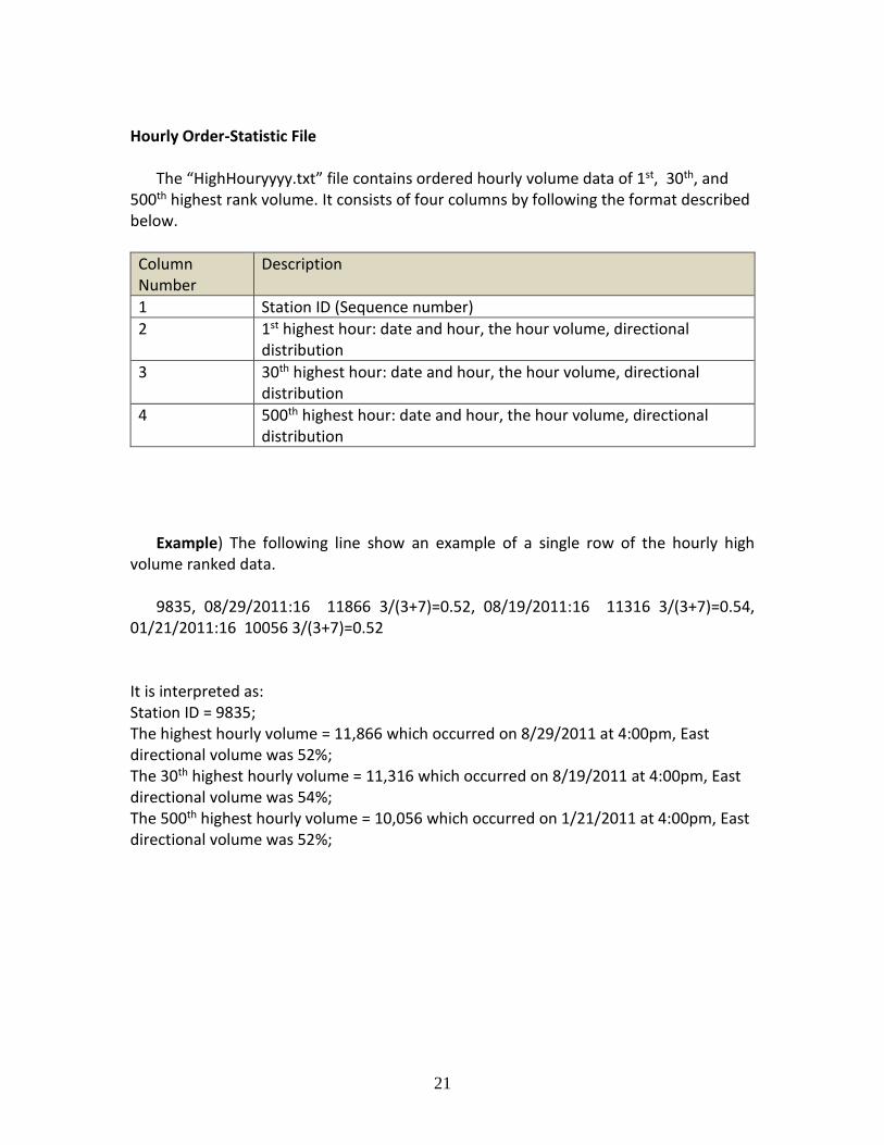
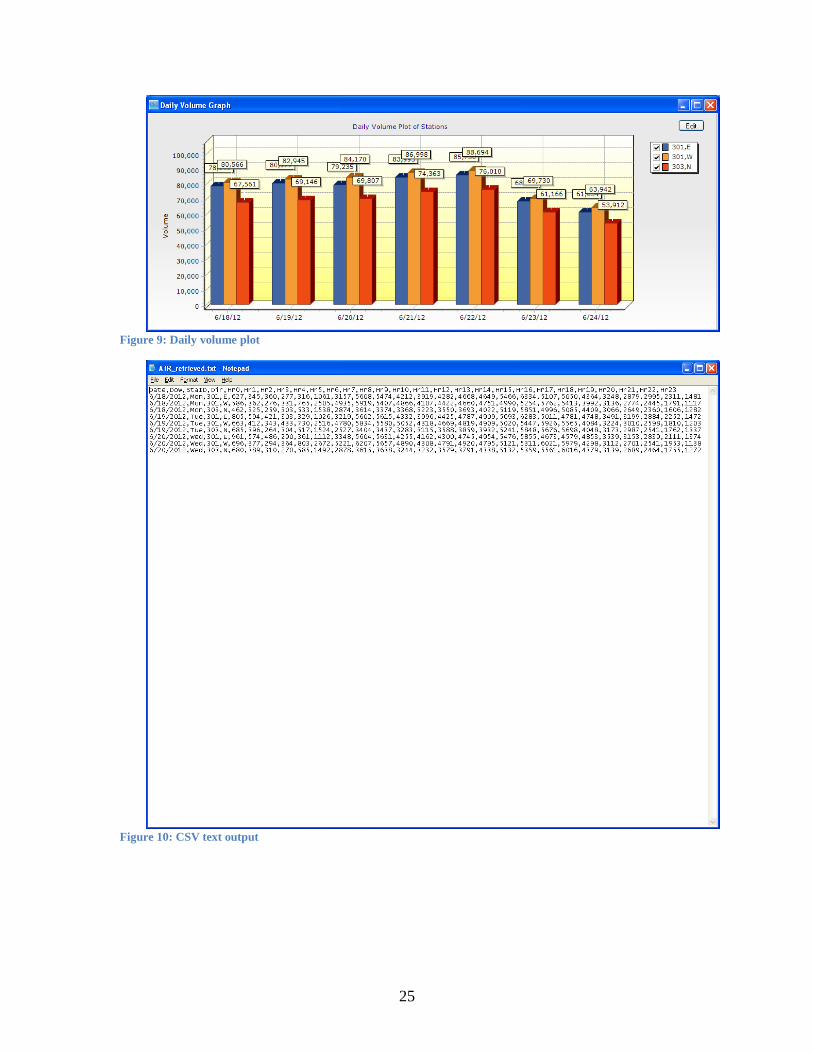
Using this tool is very simple. Please refer to the Figure 7 screen capture. First, the user needs to load an ATR file using the Browse button, which would populate the station list as well as the date list. Multiple items in the list can be selected by simultaneously pressing the Ctrl or Shift key along with the left mouse button. There are three data retrieval functions assigned to the three buttons. 1. Hourly Plot: produces hourly volumes using line plots (Figure 7) 2. Daily Plot: produces daily volume in a bar graph (Figure 8). The plot characteristics can be modified using the Edit button in the plot window. 3. Export to a File: It can produce comma separated values (CSVs) on a notepad or Excel. The column headings are shown below. The numbers, 0-23, denote total volume starting from the 0th to 23th hour of the day (Figure 9).
The ATR data file column heading of the exported file:
Date,Dow,StaID,Dir,Hr0,Hr1,Hr2,Hr3,Hr4,Hr5,Hr6,Hr7,Hr8,Hr9,Hr10,Hr11
,Hr12,Hr13,Hr14,Hr15,Hr16,Hr17,Hr18,Hr19,Hr20,Hr21,Hr22,Hr23

24
Figure 7: Screen shot of ATRviewer
Figure 8: Hourly volume plot
25
Figure 9: Daily volume plot
Figure 10: CSV text output

26
5.2 FHWA Vol Data Tab
The second tab, called FHWA Vol Data, is used to load and query FHWA formatted
volume data. Both ATR-TDA and SC-TDA include a function that produces FHWA volume data. This tab allows query and plot the hourly or daily traffic volume data. Please see Figure 11.
Figure 11: FHWA Vol Data Tab

27
5.3 SC Data Tab
When SC-TDA runs, it not only produces the final AADT data but also produces hourly
and daily traffic data for the entire year. You can use the SC Data Tab to retrieve hourly and daily traffic volumes in three forms: text, Excel, or graph. This tool is useful when you want to see hourly volumes of a day or monthly volume. It allows selection of multiple dates. A screen shot of this Tab is shown in Figure 12: left side is for hourly volume and the right side is for daily volume.
For retrieving hourly volume of a day, an hourly volume file with “.yr” or “.yrImp” extension should be loaded using the Browse button, which would populate the Stations and Dates ListBox. The user may then select one or more stations and dates. The three buttons on the right side of the dates ListBox provide retrieval options of text, Excel, or graph.
Figure 13 shows an example of the hourly plot of two consecutive dates on two selected stations as shown in Figure 12. Daily volume is retrieved using the right side
plane. Loading a daily traffic volume file (“*.days”) populates the station list. The text
and Excel outputs provide daily volume for the entire year while the plot provides the
average AADT of each month for the entire year. A example plot corresponding to
Figure 12 selection is shown in Figure 14.
Figure 12: Screen shot of SC-Query

28
Figure 13: Hourly volume plot of two stations
Figure 14: Monthly volume plot of two stations

29
6. Concluding Remark
Although the outside looks (interfaces) of the programs described in this manual show simplicity, the internal programs are complex, developed by multiple years of research and writing of thousands of lines of codes. The mathematical procedures applied for imputation may be understood at a Maters of Science (M.S.) or higher level in Engineering or in Mathematics. If anyone wishes to explore the mathematical procedures used in the software for multiple imputation, reading of the following two books are highly recommended.
[1] Rubin, Donald B., Multiple Imputation For Non-Response in Surveys, Wiley Series in
Probability and Mathematical Statistics, 1987.
[2] Little, R. J. A. and D. B. Rubin, Statistical Analysis with Missing Data, Wiley Series in
Probability and Mathematical Statistics, 1987.
The software packages will be updated regularly, typically triggered by the following
events (1) error was found, (2) operating system (OS) versions have been changed, (3) RTMC changed the data format, or (4) after a major upgrade project. Presently, the OS supported by the software are Windows XP, 7, and 10. The latest versions of the software are distributed through the web site:
http://www.d.umn.edu/~tkwon/Download/mndotDownload.htm Lastly, I would like to thank three people contributed towards this work: Mark Flinner,
Gene Hicks, and Megan Forbes. Their inputs were invaluable for research, development, and implementation of the final software packages.