Atmospheric Horizontal Resolution Affects Tropical Climate ... · in the T30 model is moderated in the T106 as it shifts to a longer time scale. At high resolution, new processes

Atmospheric Horizontal Resolution Affects Tropical Climate Variability inCoupled Models

A. NAVARRA, S. GUALDI, AND S. MASINA

Centro Euromediterraneo per i Cambiamenti Climatic, and Istituto Nazionale di Geofisica e Vulcanologia, Bologna, Italy

S. BEHERA, J.-J. LUO, AND S. MASSON

Frontier Research System for Global Change, Yokohama, Japan

E. GUILYARDI AND P. DELECLUSE

IPSL/LSCE, Gif-sur-Yvette, France

T. YAMAGATA

Frontier Research System for Global Change, Yokohama, Japan

(Manuscript received 20 March 2006, in final form 1 May 2007)

ABSTRACT

The effect of atmospheric horizontal resolution on tropical variability is investigated within the modifiedScale Interaction Experiment (SINTEX) coupled model, SINTEX-Frontier (SINTEX-F), developed jointlyat Istituto Nazionale di Geofisica e Vulcanologia (INGV), L’Institut Pierre-Simon Laplace (IPSL), and theFrontier Research System. The ocean resolution is not changed as the atmospheric model resolution ismodified from spectral resolution 30 (T30) to spectral resolution 106 (T106). The horizontal resolutions ofthe atmospheric model T30 and T106 are investigated in terms of the coupling characteristics, frequency,and variability of the tropical ocean–atmosphere interactions. It appears that the T106 resolution is gen-erally beneficial even if it does not eliminate all the major systematic errors of the coupled model. Thereis an excessive shift west of the cold tongue and ENSO variability, and high resolution also has a somewhatnegative impact on the variability in the east Indian Ocean. A dominant 2-yr peak for the Niño-3 variabilityin the T30 model is moderated in the T106 as it shifts to a longer time scale. At high resolution, newprocesses come into play, such as the coupling of tropical instability waves, the resolution of coastal flowsat the Pacific–Mexican coasts, and improved coastal forcing along the coast of South America. The delayedoscillator seems to be the main mechanism that generates the interannual variability in both models, but themodels realize it in different ways. In the T30 model it is confined close to the equator, involving relativelyfast equatorial and near-equatorial modes, and in the high-resolution model, it involves a wider latitudinalregion and slower waves. It is speculated that the extent of the region that is involved in the interannualvariability may be linked to the time scale of the variability itself.

1. Introduction

The numerical resolution of a general circulationmodel is a major factor that affects the numerical simu-lation of the atmosphere and/or the ocean. It is naturalthat considerable attention has been spent on the in-vestigation on how changing the numerical resolution

will affect the quality of the simulation. Though verticaland horizontal resolutions are probably equally impor-tant, most of the studies have focused on the horizontalresolution. The number of papers devoted to the sub-ject is very large, starting with early work at the Geo-physical Fluid Dynamics Laboratory (GFDL; Manabeet al. 1970) and continuing with later studies on theimpact of resolution for extended range (10 days),monthly, and seasonal scales (Tibaldi et al. 1990; Bo-ville 1991; Boyle 1993; Williamson et al. 1995; Brank-ovic and Gregory 2001). These studies showed that the

Corresponding author address: A. Navarra, Istituto Nazionaledi Geofisica e Vulcanologia, Via Donato Creti 12, Bologna, Italy.E-mail: [email protected]

730 J O U R N A L O F C L I M A T E VOLUME 21

DOI: 10.1175/2007JCLI1406.1

© 2008 American Meteorological Society

JCLI1406

evaluation of the effect of resolution is often difficult asthe changes in the numerics affect the components ofthe models in a complex way: overall the change tohigher resolution is beneficial, but often it is not uni-form across the model parameters and processes. Themajor systematic errors of a model cannot be elimi-nated simply by increasing resolution, even if a read-justment of the parameterization is performed (Duffyet al. 2003). Higher resolution does not appear to be amagical solution to all the illnesses of the model, butrather it defines a more advanced work field for themodeler, permitting the explicit treatment of more pro-cesses.

Several papers have investigated the impact of reso-lution, mainly horizontal resolution, for specific pro-cesses or phenomena. Bengtsson et al. (1995) showedthat simulation of tropical cyclones is more realistic atthe higher horizontal resolution considered in the study(T106). Recently, Kobayashi and Sugi (2004) haveshown that the number of simulated tropical cyclonestends to increase at an even higher resolution. Gualdi etal. (1997) investigated the impact of resolution on thesimulation of the MJO and they found that resolutionalone cannot improve the accuracy of the simulation ofthe oscillation. The simulations of the Asian summermonsoon have been shown to be sensitive to horizontalresolution (Sperber et al. 1994; Stephenson et al. 1998;Kobayashi and Sugi 2004), leading to positive results atincreased resolution. Horizontal resolution is also cru-cial to accurately treat the effects of ice sheets (Wild etal. 2003) and Greenland orography (Junge et al. 2005).

The impact of atmospheric horizontal resolution atclimate scales has received comparably less attention.Most investigations have been conducted with pre-scribed SST distribution for relatively short periods us-ing observed SST (Roeckner et al. 1996; Duffy et al.2003; Stratton 1999; Pope and Stratton 2002) or as time-slice experiments with SST from lower-resolutioncoupled models (May and Roeckner 2001; May 2003,2001).

There is almost no documentation of the effect ofatmospheric resolution in coupled models. Some as-pects of it were shown in Guilyardi et al. (2004) andGualdi et al. (2005), but a more extended study at cli-mate time scales is lacking. We present here an analysisof the interannual climate sensitivity to atmospherichorizontal resolution by examining numerical simula-tions performed with a coupled model developed by thecooperation between the Istituto Nazionale di Geo-fisica e Vulcanologia (INGV), the L’Institut Pierre-Simon Laplace (IPSL) groups, and the Frontier Groupat the Earth Simulator Center in Japan.

The focus of this paper is on the tropical coupled

dynamics. The numerical setup is such that the atmo-spheric model resolution is varied, but the ocean modelis maintained at the same resolution. We have per-formed a set of simulations with the same ocean modelcoupled to the atmospheric model at two different hori-zontal resolutions, the first truncated at spectral reso-lution 30 (T30) and the second truncated at spectralresolution 106 (T106). The simulations were of suffi-cient length to be able to establish significant statisticalresults (200 yr). Some of the aspects of the T30 vari-ability were investigated by Guilyardi et al. (2003).

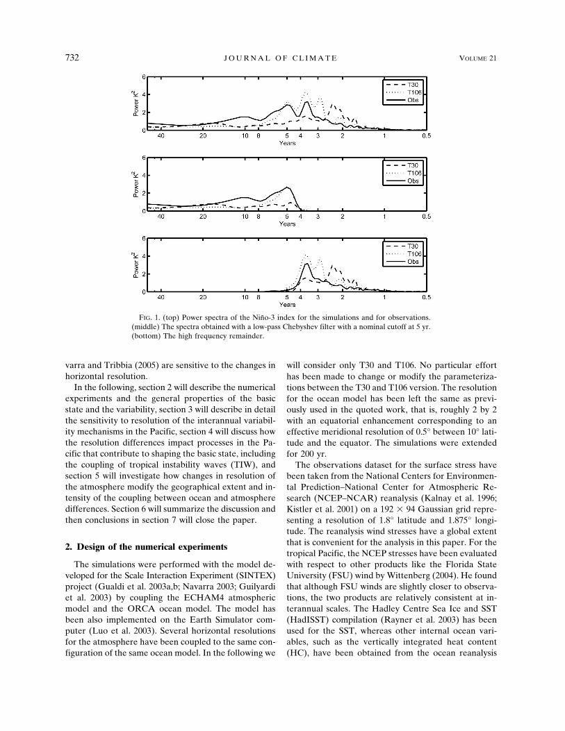
The changes in the atmospheric resolution do affectthe variability in the tropical Pacific, even if the oceanmodel has not been changed at all. The impact of thehorizontal resolution changes can be noted in a generalindicator of the tropical variability, such as the timespectrum of the Niño-3 SST index (Fig. 1). The toppanel of Fig. 1 shows that the coupled model with alow-resolution atmosphere exhibits a marked peak ofvariability around 2 yr (Guilyardi et al. 2003) and com-paratively small variability everywhere else. Thecoupled model with the high-resolution atmosphereshifts the major variability peaks toward longer timescales. The variability is overestimated with respect tothe observations and there are still some remains of themisplaced peak at around 2 yr, but there is a noticeableimprovement. In the following we will refer to thesetwo experiments as the low- and high-resolution experi-ments, respectively.

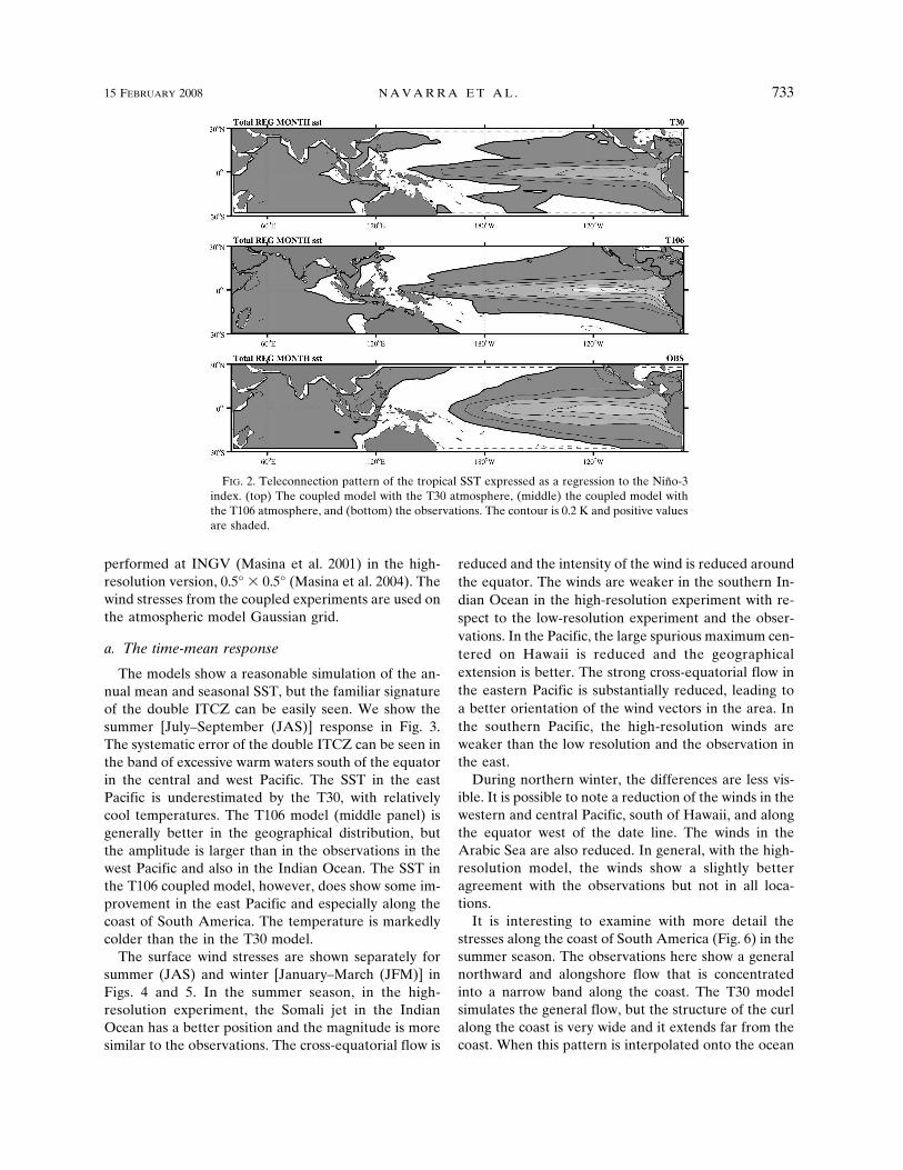
The improved horizontal resolution impacts also theteleconnections properties of the variability (Fig. 2).The regression pattern in the observation of the Niño-3SST index with the SST elsewhere is a wide wedgepattern protruding into the Pacific Ocean. The low-resolution model displays a regression pattern that isweaker in total amplitude and it is more confined to theequator than the observations, whereas the high reso-lution is showing a higher amplitude and a wider pat-tern in latitude. Though the main systematic errors inthe teleconnection are not automatically solved by theshift to high resolution, we can see that the higher-resolution coupled model yields a more realistic patternand indicates a general beneficial trend.

Modifying the atmospheric resolution, therefore, af-fects the ocean behavior and ocean variables even if theocean model is not modified in the coupling.

In the following, we will investigate the mechanismsthat allow this effect to take place. We will characterizethe time-mean patterns of the models and their vari-ability, the wave propagation, and the changes in thecoupling properties of the models. We will investigatehow the interannual variability, the teleconnectionsproperties, and the coupled manifold introduced by Na-

15 FEBRUARY 2008 N A V A R R A E T A L . 731

varra and Tribbia (2005) are sensitive to the changes inhorizontal resolution.

In the following, section 2 will describe the numericalexperiments and the general properties of the basicstate and the variability, section 3 will describe in detailthe sensitivity to resolution of the interannual variabil-ity mechanisms in the Pacific, section 4 will discuss howthe resolution differences impact processes in the Pa-cific that contribute to shaping the basic state, includingthe coupling of tropical instability waves (TIW), andsection 5 will investigate how changes in resolution ofthe atmosphere modify the geographical extent and in-tensity of the coupling between ocean and atmospheredifferences. Section 6 will summarize the discussion andthen conclusions in section 7 will close the paper.

2. Design of the numerical experiments

The simulations were performed with the model de-veloped for the Scale Interaction Experiment (SINTEX)project (Gualdi et al. 2003a,b; Navarra 2003; Guilyardiet al. 2003) by coupling the ECHAM4 atmosphericmodel and the ORCA ocean model. The model hasbeen also implemented on the Earth Simulator com-puter (Luo et al. 2003). Several horizontal resolutionsfor the atmosphere have been coupled to the same con-figuration of the same ocean model. In the following we

will consider only T30 and T106. No particular efforthas been made to change or modify the parameteriza-tions between the T30 and T106 version. The resolutionfor the ocean model has been left the same as previ-ously used in the quoted work, that is, roughly 2 by 2with an equatorial enhancement corresponding to aneffective meridional resolution of 0.5° between 10° lati-tude and the equator. The simulations were extendedfor 200 yr.

The observations dataset for the surface stress havebeen taken from the National Centers for Environmen-tal Prediction–National Center for Atmospheric Re-search (NCEP–NCAR) reanalysis (Kalnay et al. 1996;Kistler et al. 2001) on a 192 � 94 Gaussian grid repre-senting a resolution of 1.8° latitude and 1.875° longi-tude. The reanalysis wind stresses have a global extentthat is convenient for the analysis in this paper. For thetropical Pacific, the NCEP stresses have been evaluatedwith respect to other products like the Florida StateUniversity (FSU) wind by Wittenberg (2004). He foundthat although FSU winds are slightly closer to observa-tions, the two products are relatively consistent at in-terannual scales. The Hadley Centre Sea Ice and SST(HadISST) compilation (Rayner et al. 2003) has beenused for the SST, whereas other internal ocean vari-ables, such as the vertically integrated heat content(HC), have been obtained from the ocean reanalysis

FIG. 1. (top) Power spectra of the Niño-3 index for the simulations and for observations.(middle) The spectra obtained with a low-pass Chebyshev filter with a nominal cutoff at 5 yr.(bottom) The high frequency remainder.


performed at INGV (Masina et al. 2001) in the high-resolution version, 0.5° � 0.5° (Masina et al. 2004). Thewind stresses from the coupled experiments are used onthe atmospheric model Gaussian grid.

a. The time-mean response

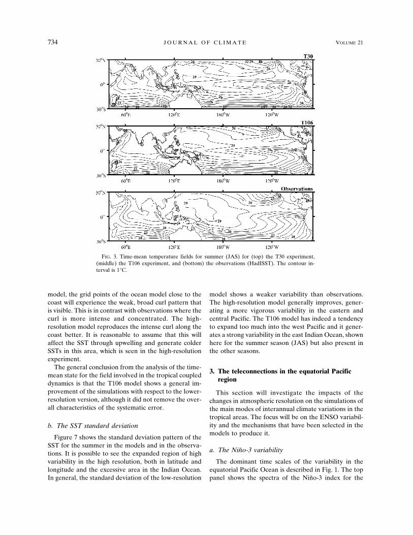
The models show a reasonable simulation of the an-nual mean and seasonal SST, but the familiar signatureof the double ITCZ can be easily seen. We show thesummer [July–September (JAS)] response in Fig. 3.The systematic error of the double ITCZ can be seen inthe band of excessive warm waters south of the equatorin the central and west Pacific. The SST in the eastPacific is underestimated by the T30, with relativelycool temperatures. The T106 model (middle panel) isgenerally better in the geographical distribution, butthe amplitude is larger than in the observations in thewest Pacific and also in the Indian Ocean. The SST inthe T106 coupled model, however, does show some im-provement in the east Pacific and especially along thecoast of South America. The temperature is markedlycolder than the in the T30 model.

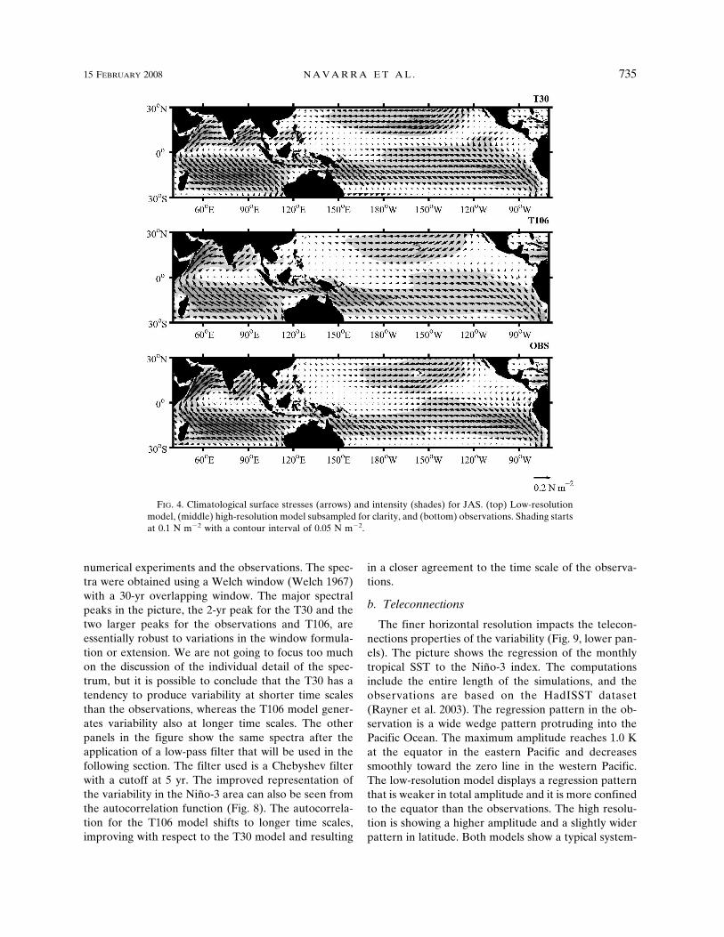
The surface wind stresses are shown separately forsummer (JAS) and winter [January–March (JFM)] inFigs. 4 and 5. In the summer season, in the high-resolution experiment, the Somali jet in the IndianOcean has a better position and the magnitude is moresimilar to the observations. The cross-equatorial flow is

reduced and the intensity of the wind is reduced aroundthe equator. The winds are weaker in the southern In-dian Ocean in the high-resolution experiment with re-spect to the low-resolution experiment and the obser-vations. In the Pacific, the large spurious maximum cen-tered on Hawaii is reduced and the geographicalextension is better. The strong cross-equatorial flow inthe eastern Pacific is substantially reduced, leading toa better orientation of the wind vectors in the area. Inthe southern Pacific, the high-resolution winds areweaker than the low resolution and the observation inthe east.

During northern winter, the differences are less vis-ible. It is possible to note a reduction of the winds in thewestern and central Pacific, south of Hawaii, and alongthe equator west of the date line. The winds in theArabic Sea are also reduced. In general, with the high-resolution model, the winds show a slightly betteragreement with the observations but not in all loca-tions.

It is interesting to examine with more detail thestresses along the coast of South America (Fig. 6) in thesummer season. The observations here show a generalnorthward and alongshore flow that is concentratedinto a narrow band along the coast. The T30 modelsimulates the general flow, but the structure of the curlalong the coast is very wide and it extends far from thecoast. When this pattern is interpolated onto the ocean

FIG. 2. Teleconnection pattern of the tropical SST expressed as a regression to the Niño-3index. (top) The coupled model with the T30 atmosphere, (middle) the coupled model withthe T106 atmosphere, and (bottom) the observations. The contour is 0.2 K and positive valuesare shaded.


model, the grid points of the ocean model close to thecoast will experience the weak, broad curl pattern thatis visible. This is in contrast with observations where thecurl is more intense and concentrated. The high-resolution model reproduces the intense curl along thecoast better. It is reasonable to assume that this willaffect the SST through upwelling and generate colderSSTs in this area, which is seen in the high-resolutionexperiment.

The general conclusion from the analysis of the time-mean state for the field involved in the tropical coupleddynamics is that the T106 model shows a general im-provement of the simulations with respect to the lower-resolution version, although it did not remove the over-all characteristics of the systematic error.

b. The SST standard deviation

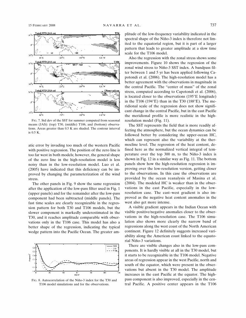
Figure 7 shows the standard deviation pattern of theSST for the summer in the models and in the observa-tions. It is possible to see the expanded region of highvariability in the high resolution, both in latitude andlongitude and the excessive area in the Indian Ocean.In general, the standard deviation of the low-resolution

model shows a weaker variability than observations.The high-resolution model generally improves, gener-ating a more vigorous variability in the eastern andcentral Pacific. The T106 model has indeed a tendencyto expand too much into the west Pacific and it gener-ates a strong variability in the east Indian Ocean, shownhere for the summer season (JAS) but also present inthe other seasons.

3. The teleconnections in the equatorial Pacificregion

This section will investigate the impacts of thechanges in atmospheric resolution on the simulations ofthe main modes of interannual climate variations in thetropical areas. The focus will be on the ENSO variabil-ity and the mechanisms that have been selected in themodels to produce it.

a. The Niño-3 variability

The dominant time scales of the variability in theequatorial Pacific Ocean is described in Fig. 1. The toppanel shows the spectra of the Niño-3 index for the

FIG. 3. Time-mean temperature fields for summer (JAS) for (top) the T30 experiment,(middle) the T106 experiment, and (bottom) the observations (HadISST). The contour in-terval is 1°C.


numerical experiments and the observations. The spec-tra were obtained using a Welch window (Welch 1967)with a 30-yr overlapping window. The major spectralpeaks in the picture, the 2-yr peak for the T30 and thetwo larger peaks for the observations and T106, areessentially robust to variations in the window formula-tion or extension. We are not going to focus too muchon the discussion of the individual detail of the spec-trum, but it is possible to conclude that the T30 has atendency to produce variability at shorter time scalesthan the observations, whereas the T106 model gener-ates variability also at longer time scales. The otherpanels in the figure show the same spectra after theapplication of a low-pass filter that will be used in thefollowing section. The filter used is a Chebyshev filterwith a cutoff at 5 yr. The improved representation ofthe variability in the Niño-3 area can also be seen fromthe autocorrelation function (Fig. 8). The autocorrela-tion for the T106 model shifts to longer time scales,improving with respect to the T30 model and resulting

in a closer agreement to the time scale of the observa-tions.

b. Teleconnections

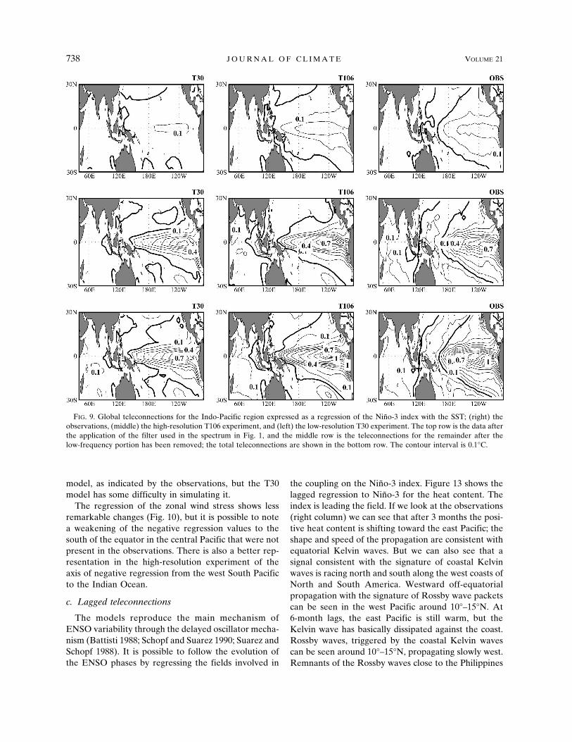
The finer horizontal resolution impacts the telecon-nections properties of the variability (Fig. 9, lower pan-els). The picture shows the regression of the monthlytropical SST to the Niño-3 index. The computationsinclude the entire length of the simulations, and theobservations are based on the HadISST dataset(Rayner et al. 2003). The regression pattern in the ob-servation is a wide wedge pattern protruding into thePacific Ocean. The maximum amplitude reaches 1.0 Kat the equator in the eastern Pacific and decreasessmoothly toward the zero line in the western Pacific.The low-resolution model displays a regression patternthat is weaker in total amplitude and it is more confinedto the equator than the observations. The high resolu-tion is showing a higher amplitude and a slightly widerpattern in latitude. Both models show a typical system-

FIG. 4. Climatological surface stresses (arrows) and intensity (shades) for JAS. (top) Low-resolutionmodel, (middle) high-resolution model subsampled for clarity, and (bottom) observations. Shading startsat 0.1 N m�2 with a contour interval of 0.05 N m�2.


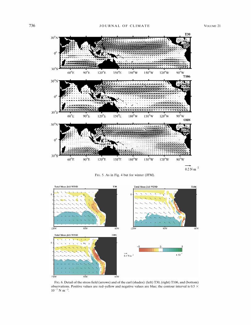
FIG. 5. As in Fig. 4 but for winter (JFM).

FIG. 6. Detail of the stress field (arrows) and of the curl (shades): (left) T30, (right) T106, and (bottom)observations. Positive values are red–yellow and negative values are blue; the contour interval is 0.5 �10�7 N m�3.


Fig 6 live 4/C

atic error by invading too much of the western Pacificwith positive regression. The position of the zero line istoo far west in both models; however, the general shapeof the zero line in the high-resolution model is lessnoisy than in the low-resolution model. Luo et al.(2005) have indicated that this deficiency can be im-proved by changing the parameterization of the windstress.

The other panels in Fig. 9 show the same regressionafter the application of the low-pass filter used in Fig. 1(upper panels) and for the remainder after the low-passcomponent had been subtracted (middle panels). Thefast time scales are clearly recognizable in the regres-sion pattern for both T30 and T106 models, but theslower component is markedly underestimated in theT30, and it reaches amplitude comparable with obser-vations only in the T106 case. This model has also abetter shape of the regression, indicating the typicalwedge pattern into the Pacific Ocean. The greater am-

plitude of the low-frequency variability indicated in thespectral shape of the Niño-3 index is therefore not lim-ited to the equatorial region, but it is part of a largerpattern that leads to greater amplitude at a slow timescale for the T106 model.

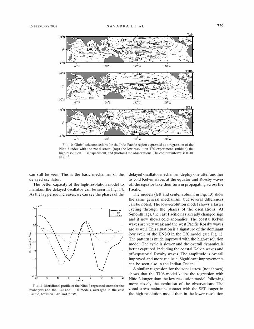
Also the regression with the zonal stress shows someimprovements. Figure 10 shows the regression of thezonal wind stress to Niño-3 SST index. A bandpass fil-ter between 1 and 5 yr has been applied following Ca-potondi et al. (2006). The high-resolution model has abetter agreement with the observations in magnitude inthe central Pacific. The “center of mass” of the zonalstress, computed according to Capotondi et al. (2006),is located closer to the observations (195°E longitude)in the T106 (194°E) than in the T30 (188°E). The me-ridional scale of the regression does not show signifi-cant change in the central Pacific, but in the east Pacificthe meridional profile is more realistic in the high-resolution model (Fig. 11).

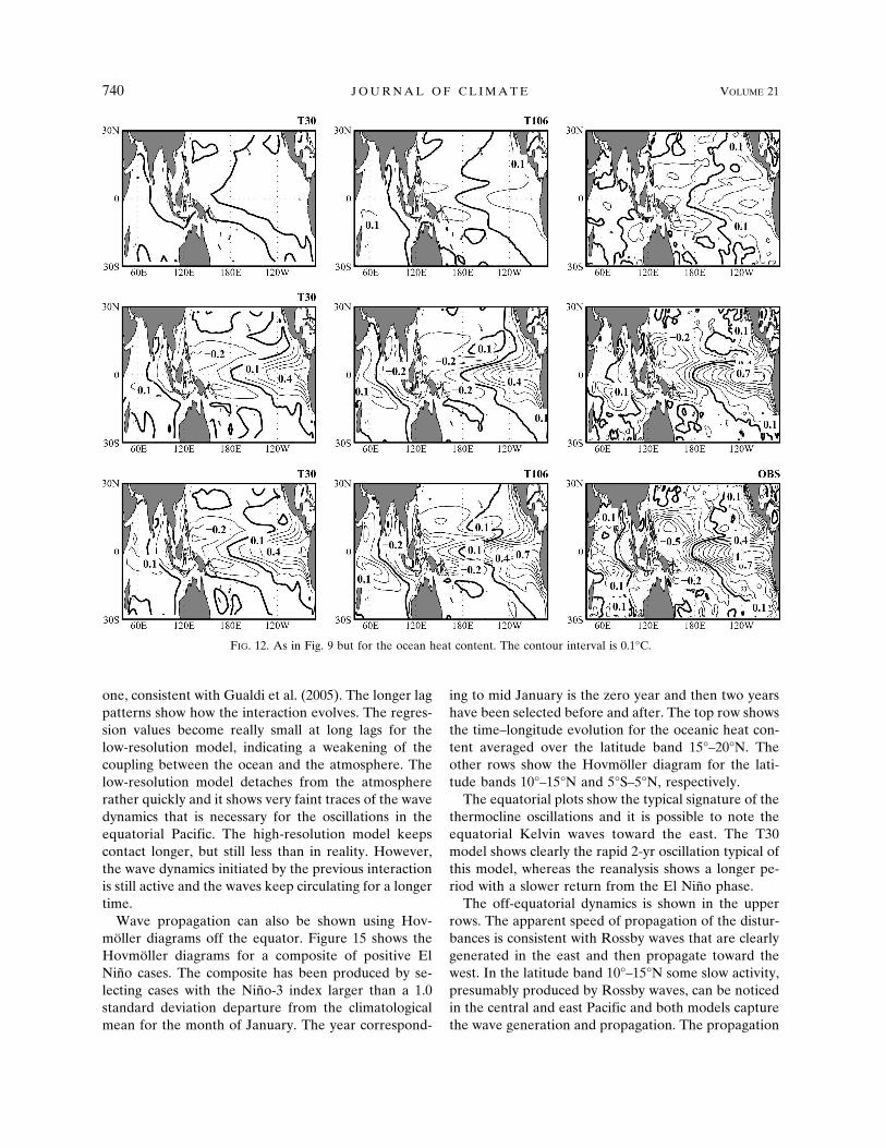
The SST represents the field that is more readily af-fecting the atmosphere, but the ocean dynamics can befollowed better by considering the upper-ocean HC,which can represent also the variability at the ther-mocline level. The regression of the heat content, de-fined here as the normalized vertical integral of tem-perature over the top 300 m, to the Niño-3 index isshown in Fig. 12 in a similar way as Fig. 11. The bottompanels show how the high-resolution regression is im-proving over the low-resolution version, getting closerto the observations. In this case the observations areprovided by the ocean reanalysis of Masina et al.(2004). The modeled HC is weaker than in the obser-vations in the east Pacific, especially in the low-resolution case. The east–west gradient is also im-proved as the negative heat content anomalies in thewest also get more intense.

A visible gradient appears in the Indian Ocean withvisible positive/negative anomalies closer to the obser-vations in the high-resolution case. The T106 simu-lation also shows more clearly the narrow band ofregressions along the west coast of the North Americancontinent. Figure 12 definitely suggests increased vari-ability along the American coast linked to the equato-rial Niño-3 variations.

There are visible changes also in the low-pass com-ponents. It is hardly visible at all in the T30 model, butit starts to be recognizable in the T106 model. Negativeareas of regression appear in the west Pacific, north andsouth of the equator, which were present in the obser-vations but absent in the T30 model. The amplitudeincreases in the east Pacific at the equator. The high-pass component is also improved, especially in the cen-tral Pacific. A positive center appears in the T106

FIG. 8. Autocorrelation of the Niño-3 index for the T30 andT106 model simulations and for the observations.

FIG. 7. Std dev of the SST for summer computed from seasonalmeans (JAS): (top) T30, (middle) T106, and (bottom) observa-tions. Areas greater than 0.5 K are shaded. The contour intervalis 0.5 K.


model, as indicated by the observations, but the T30model has some difficulty in simulating it.

The regression of the zonal wind stress shows lessremarkable changes (Fig. 10), but it is possible to notea weakening of the negative regression values to thesouth of the equator in the central Pacific that were notpresent in the observations. There is also a better rep-resentation in the high-resolution experiment of theaxis of negative regression from the west South Pacificto the Indian Ocean.

c. Lagged teleconnections

The models reproduce the main mechanism ofENSO variability through the delayed oscillator mecha-nism (Battisti 1988; Schopf and Suarez 1990; Suarez andSchopf 1988). It is possible to follow the evolution ofthe ENSO phases by regressing the fields involved in

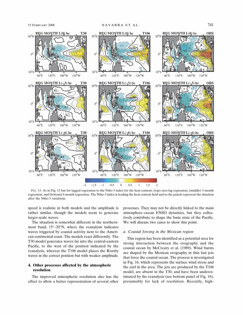
the coupling on the Niño-3 index. Figure 13 shows thelagged regression to Niño-3 for the heat content. Theindex is leading the field. If we look at the observations(right column) we can see that after 3 months the posi-tive heat content is shifting toward the east Pacific; theshape and speed of the propagation are consistent withequatorial Kelvin waves. But we can also see that asignal consistent with the signature of coastal Kelvinwaves is racing north and south along the west coasts ofNorth and South America. Westward off-equatorialpropagation with the signature of Rossby wave packetscan be seen in the west Pacific around 10°–15°N. At6-month lags, the east Pacific is still warm, but theKelvin wave has basically dissipated against the coast.Rossby waves, triggered by the coastal Kelvin wavescan be seen around 10°–15°N, propagating slowly west.Remnants of the Rossby waves close to the Philippines

FIG. 9. Global teleconnections for the Indo-Pacific region expressed as a regression of the Niño-3 index with the SST; (right) theobservations, (middle) the high-resolution T106 experiment, and (left) the low-resolution T30 experiment. The top row is the data afterthe application of the filter used in the spectrum in Fig. 1, and the middle row is the teleconnections for the remainder after thelow-frequency portion has been removed; the total teleconnections are shown in the bottom row. The contour interval is 0.1°C.


can still be seen. This is the basic mechanism of thedelayed oscillator.

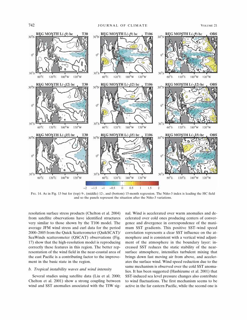
The better capacity of the high-resolution model tomaintain the delayed oscillator can be seen in Fig. 14.As the lag period increases, we can see the phases of the

delayed oscillator mechanism deploy one after anotheras cold Kelvin waves at the equator and Rossby wavesoff the equator take their turn in propagating across thePacific.

The models (left and center column in Fig. 13) showthe same general mechanism, but several differencescan be noted. The low-resolution model shows a fastercycling through the phases of the oscillations. At6-month lags, the east Pacific has already changed signand it now shows cold anomalies. The coastal Kelvinwaves are very weak and the west Pacific Rossby wavesare as well. This situation is a signature of the dominant2-yr cycle of the ENSO in the T30 model (see Fig. 1).The pattern is much improved with the high-resolutionmodel. The cycle is slower and the overall dynamics isbetter captured, including the coastal Kelvin waves andoff-equatorial Rossby waves. The amplitude is overallimproved and more realistic. Significant improvementscan be seen also in the Indian Ocean.

A similar regression for the zonal stress (not shown)shows that the T106 model keeps the regression withNiño-3 longer than the low-resolution model, followingmore closely the evolution of the observations. Thezonal stress maintains contact with the SST longer inthe high-resolution model than in the lower-resolution

FIG. 11. Meridional profile of the Niño-3 regressed stress for thereanalysis and the T30 and T106 models, averaged in the eastPacific, between 120° and 90°W.

FIG. 10. Global teleconnections for the Indo-Pacific region expressed as a regression of theNiño-3 index with the zonal stress; (top) the low-resolution T30 experiment, (middle) thehigh-resolution T106 experiment, and (bottom) the observations. The contour interval is 0.001N m�2.


one, consistent with Gualdi et al. (2005). The longer lagpatterns show how the interaction evolves. The regres-sion values become really small at long lags for thelow-resolution model, indicating a weakening of thecoupling between the ocean and the atmosphere. Thelow-resolution model detaches from the atmosphererather quickly and it shows very faint traces of the wavedynamics that is necessary for the oscillations in theequatorial Pacific. The high-resolution model keepscontact longer, but still less than in reality. However,the wave dynamics initiated by the previous interactionis still active and the waves keep circulating for a longertime.

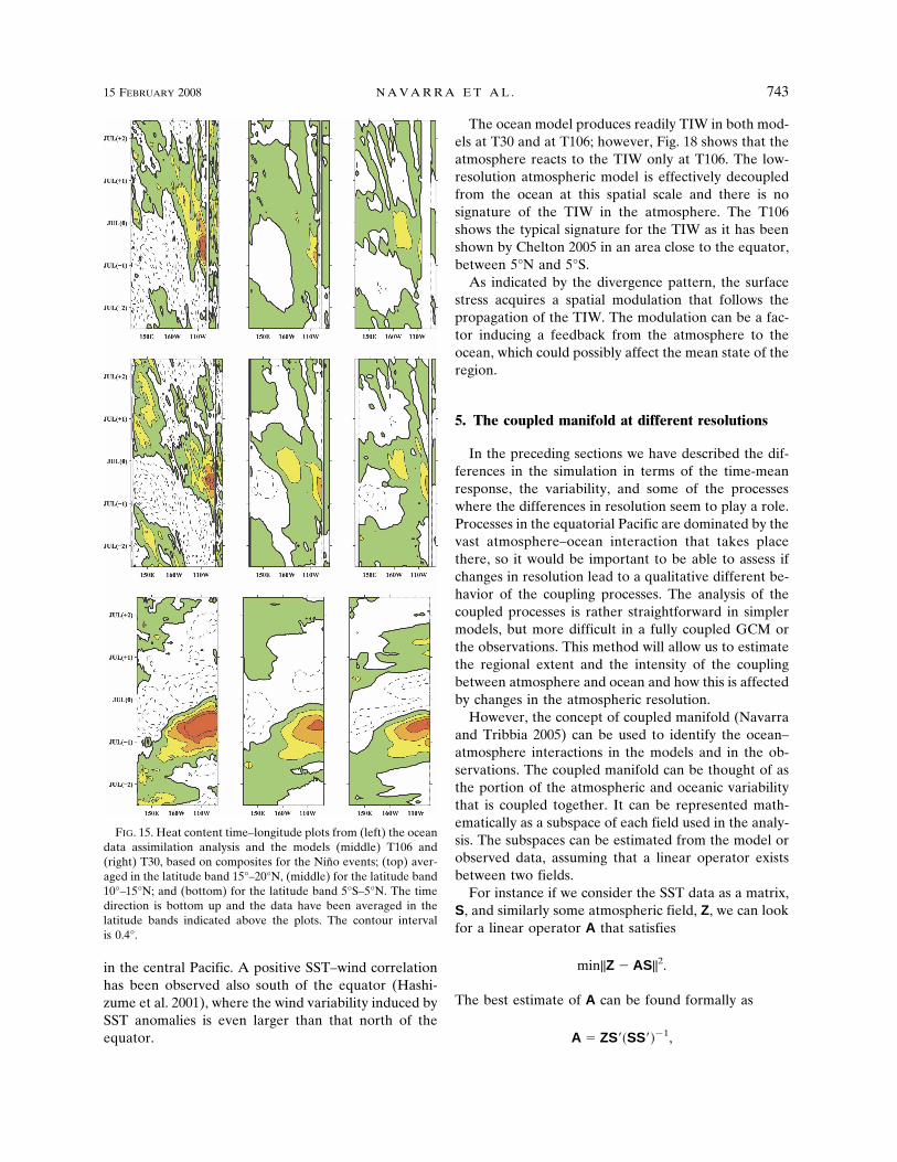
Wave propagation can also be shown using Hov-möller diagrams off the equator. Figure 15 shows theHovmöller diagrams for a composite of positive ElNiño cases. The composite has been produced by se-lecting cases with the Niño-3 index larger than a 1.0standard deviation departure from the climatologicalmean for the month of January. The year correspond-

ing to mid January is the zero year and then two yearshave been selected before and after. The top row showsthe time–longitude evolution for the oceanic heat con-tent averaged over the latitude band 15°–20°N. Theother rows show the Hovmöller diagram for the lati-tude bands 10°–15°N and 5°S–5°N, respectively.

The equatorial plots show the typical signature of thethermocline oscillations and it is possible to note theequatorial Kelvin waves toward the east. The T30model shows clearly the rapid 2-yr oscillation typical ofthis model, whereas the reanalysis shows a longer pe-riod with a slower return from the El Niño phase.

The off-equatorial dynamics is shown in the upperrows. The apparent speed of propagation of the distur-bances is consistent with Rossby waves that are clearlygenerated in the east and then propagate toward thewest. In the latitude band 10°–15°N some slow activity,presumably produced by Rossby waves, can be noticedin the central and east Pacific and both models capturethe wave generation and propagation. The propagation

FIG. 12. As in Fig. 9 but for the ocean heat content. The contour interval is 0.1°C.


speed is realistic in both models and the amplitude israther similar, though the models seem to generatelarger-scale waves.

The situation is somewhat different in the northern-most band, 15°–20°N, where the reanalysis indicateswaves triggered by coastal activity next to the Ameri-can continental coast. The models react differently. TheT30 model generates waves far into the central-easternPacific, to the west of the position indicated by thereanalysis, whereas the T106 model places the Rossbywaves in the correct position but with weaker amplitude.

4. Other processes affected by the atmosphericresolution

The improved atmospheric resolution also has theeffect to allow a better representation of several other

processes. They may not be directly linked to the mainatmosphere–ocean ENSO dynamics, but they collec-tively contribute to shape the basic state of the Pacific.We will discuss two cases to show this point.

a. Coastal forcing in the Mexican region

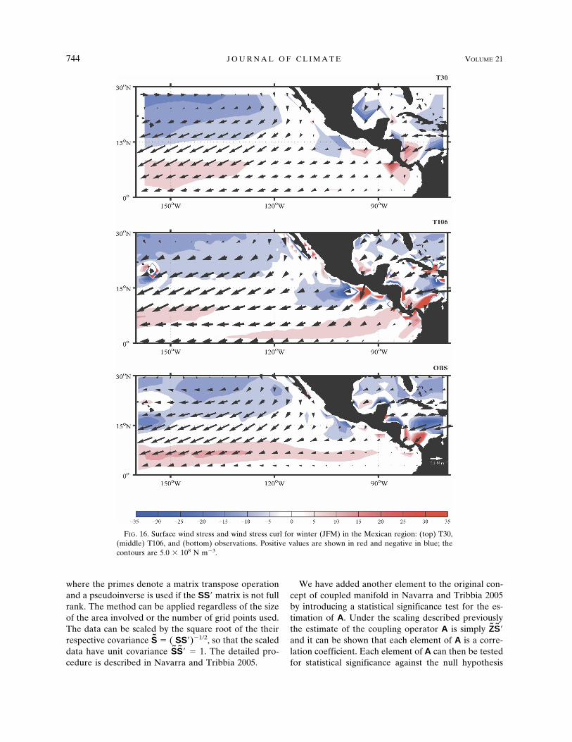
This region has been identified as a potential area forstrong interaction between the orography and thecoastal ocean by McCreary et al. (1989). Wind burstsare shaped by the Mexican orography in thin fast jetsthat force the coastal ocean. The process is investigatedin Fig. 16, which represents the surface wind stress andthe curl in the area. The jets are produced by the T106model, are absent in the T30, and have been underes-timated by the reanalysis (see bottom panel of Fig. 16),presumably for lack of resolution. Recently, high-

FIG. 13. As in Fig. 12 but for lagged regression to the Niño-3 index for the heat content; (top) zero-lag regression, (middle) 3-monthregression, and (bottom) 6-month regression. The Niño-3 index is leading the heat content field and so the panels represent the situationafter the Niño-3 variations.


Fig 13 live 4/C

resolution surface stress products (Chelton et al. 2004)from satellite observations have identified structuresvery similar to those shown by the T106 model. Theaverage JFM wind stress and curl data for the period2000–2005 from the Quick Scatterometer (QuikSCAT)/SeaWinds scatterometer (QSCAT) observations (Fig.17) show that the high-resolution model is reproducingcorrectly these features in this region. The better rep-resentation of the wind field in the near-coastal area ofthe east Pacific is a contributing factor to the improve-ment in the basic state in the region.

b. Tropical instability waves and wind intensity

Several studies using satellite data (Liu et al. 2000;Chelton et al. 2001) show a strong coupling betweenwind and SST anomalies associated with the TIW sig-

nal. Wind is accelerated over warm anomalies and de-celerated over cold ones producing centers of conver-gence and divergence in correspondence of the maxi-mum SST gradients. This positive SST–wind speedcorrelation represents a clear SST influence on the at-mosphere and is consistent with a vertical wind adjust-ment of the atmosphere in the boundary layer: in-creased SST reduces the static stability of the near-surface atmosphere, intensifies turbulent mixing thatbrings down fast moving air from above, and acceler-ates the surface wind. Wind speed reduction due to thesame mechanism is observed over the cold SST anoma-lies. It has been suggested (Hashizume et al. 2001) thatSST-induced sea level pressure changes also contributeto wind fluctuations. The first mechanism seems to beactive in the far eastern Pacific, while the second one is

FIG. 14. As in Fig. 13 but for (top) 9-, (middle) 12-, and (bottom) 15-month regression. The Niño-3 index is leading the HC fieldand so the panels represent the situation after the Niño-3 variations.


Fig 14 live 4/C

in the central Pacific. A positive SST–wind correlationhas been observed also south of the equator (Hashi-zume et al. 2001), where the wind variability induced bySST anomalies is even larger than that north of theequator.

The ocean model produces readily TIW in both mod-els at T30 and at T106; however, Fig. 18 shows that theatmosphere reacts to the TIW only at T106. The low-resolution atmospheric model is effectively decoupledfrom the ocean at this spatial scale and there is nosignature of the TIW in the atmosphere. The T106shows the typical signature for the TIW as it has beenshown by Chelton 2005 in an area close to the equator,between 5°N and 5°S.

As indicated by the divergence pattern, the surfacestress acquires a spatial modulation that follows thepropagation of the TIW. The modulation can be a fac-tor inducing a feedback from the atmosphere to theocean, which could possibly affect the mean state of theregion.

5. The coupled manifold at different resolutions

In the preceding sections we have described the dif-ferences in the simulation in terms of the time-meanresponse, the variability, and some of the processeswhere the differences in resolution seem to play a role.Processes in the equatorial Pacific are dominated by thevast atmosphere–ocean interaction that takes placethere, so it would be important to be able to assess ifchanges in resolution lead to a qualitative different be-havior of the coupling processes. The analysis of thecoupled processes is rather straightforward in simplermodels, but more difficult in a fully coupled GCM orthe observations. This method will allow us to estimatethe regional extent and the intensity of the couplingbetween atmosphere and ocean and how this is affectedby changes in the atmospheric resolution.

However, the concept of coupled manifold (Navarraand Tribbia 2005) can be used to identify the ocean–atmosphere interactions in the models and in the ob-servations. The coupled manifold can be thought of asthe portion of the atmospheric and oceanic variabilitythat is coupled together. It can be represented math-ematically as a subspace of each field used in the analy-sis. The subspaces can be estimated from the model orobserved data, assuming that a linear operator existsbetween two fields.

For instance if we consider the SST data as a matrix,S, and similarly some atmospheric field, Z, we can lookfor a linear operator A that satisfies

min||Z � AS||2.

The best estimate of A can be found formally as

A � ZS��SS��1,

FIG. 15. Heat content time–longitude plots from (left) the oceandata assimilation analysis and the models (middle) T106 and(right) T30, based on composites for the Niño events; (top) aver-aged in the latitude band 15°–20°N, (middle) for the latitude band10°–15°N; and (bottom) for the latitude band 5°S–5°N. The timedirection is bottom up and the data have been averaged in thelatitude bands indicated above the plots. The contour intervalis 0.4°.


Fig 15 live 4/C

where the primes denote a matrix transpose operationand a pseudoinverse is used if the SS� matrix is not fullrank. The method can be applied regardless of the sizeof the area involved or the number of grid points used.The data can be scaled by the square root of the theirrespective covariance S̃ � ( SS�)�1/2, so that the scaleddata have unit covariance S̃S̃� � 1. The detailed pro-cedure is described in Navarra and Tribbia 2005.

We have added another element to the original con-cept of coupled manifold in Navarra and Tribbia 2005by introducing a statistical significance test for the es-timation of A. Under the scaling described previouslythe estimate of the coupling operator A is simply Z̃S̃�and it can be shown that each element of A is a corre-lation coefficient. Each element of A can then be testedfor statistical significance against the null hypothesis

FIG. 16. Surface wind stress and wind stress curl for winter (JFM) in the Mexican region: (top) T30,(middle) T106, and (bottom) observations. Positive values are shown in red and negative in blue; thecontours are 5.0 � 108 N m�3.


Fig 16 live 4/C

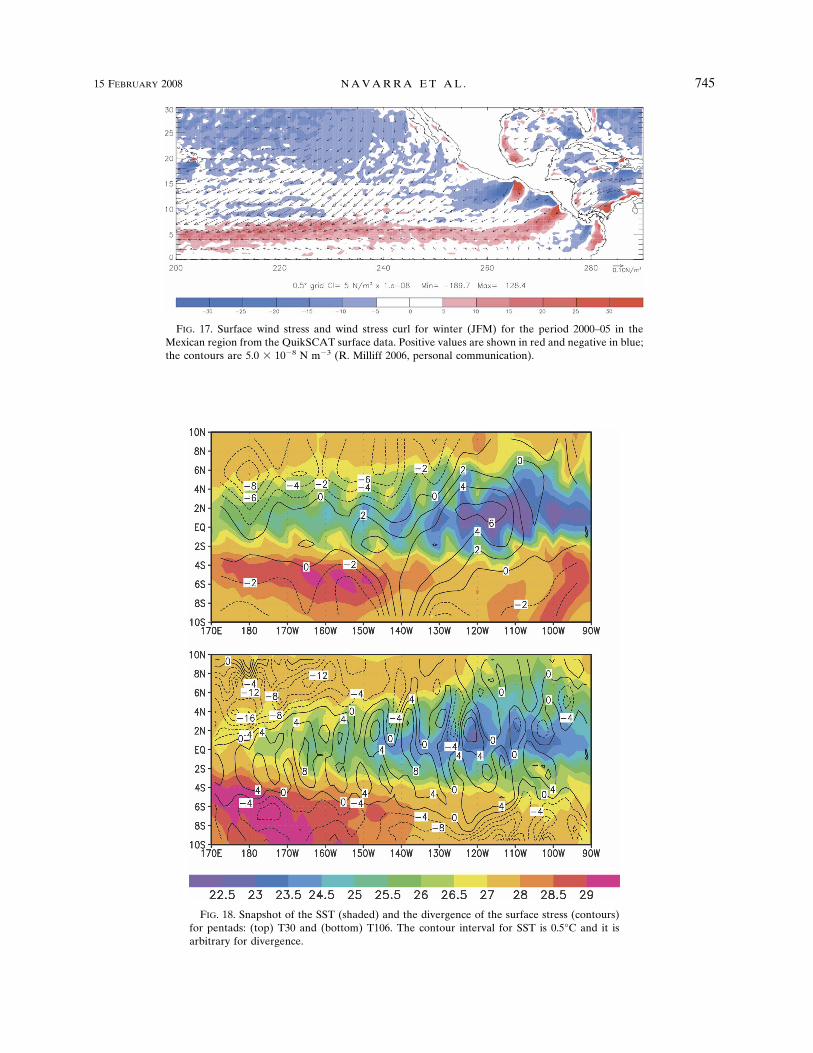
FIG. 17. Surface wind stress and wind stress curl for winter (JFM) for the period 2000–05 in theMexican region from the QuikSCAT surface data. Positive values are shown in red and negative in blue;the contours are 5.0 � 10�8 N m�3 (R. Milliff 2006, personal communication).

FIG. 18. Snapshot of the SST (shaded) and the divergence of the surface stress (contours)for pentads: (top) T30 and (bottom) T106. The contour interval for SST is 0.5°C and it isarbitrary for divergence.


Fig 17 18 live 4/C

that the correlation is zero. In the following, only thecoefficients that passed a 5% significance criterion havebeen retained in the construction of the coupling op-erator A.

a. SST and wind stress

This method can separate the time series of each fieldin the part that is cross correlated with the other. Theresulting time series can then be used for further pro-cessing. In the following we have considered the ratio ofvariance of the cross-correlated portion with respect tothe total to yield an estimate of the strength of thecoupling relation. We have considered instantaneousrelation, but the generalization to the lagged case isimmediate.

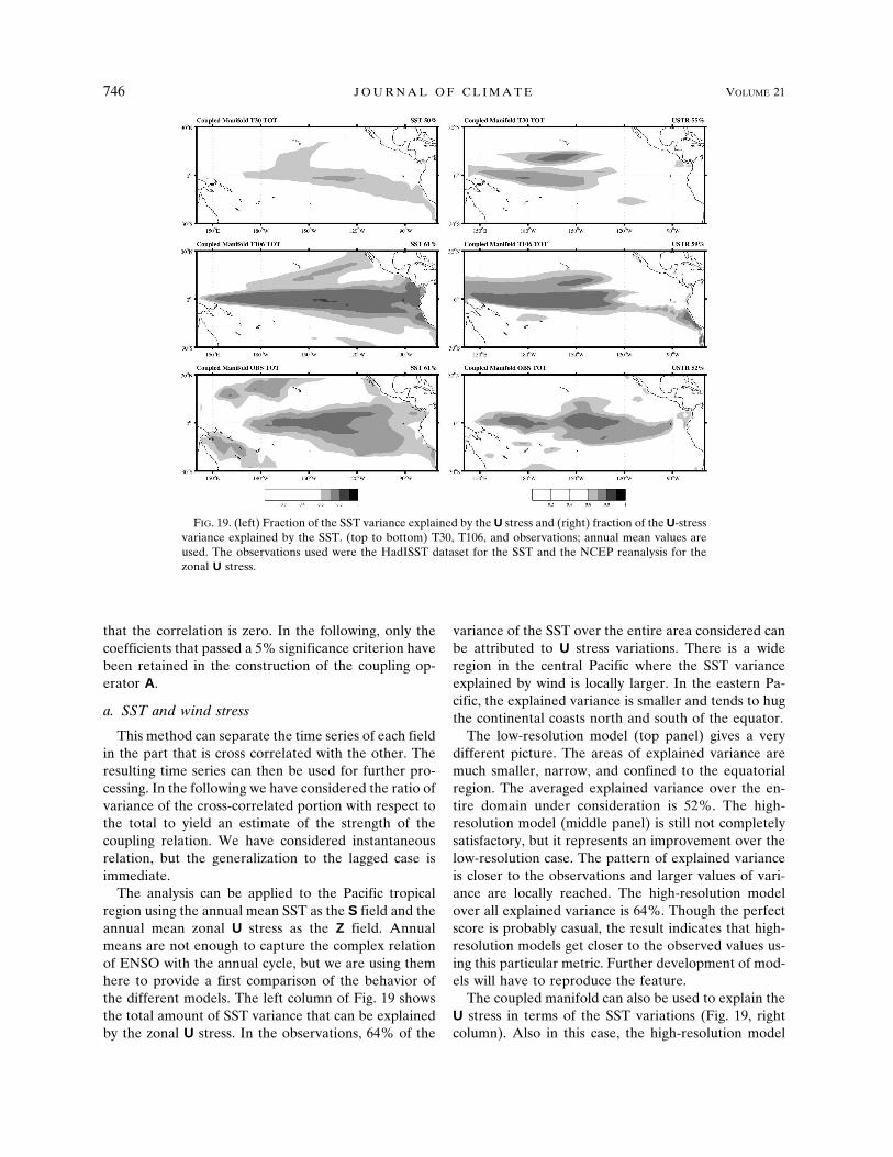
The analysis can be applied to the Pacific tropicalregion using the annual mean SST as the S field and theannual mean zonal U stress as the Z field. Annualmeans are not enough to capture the complex relationof ENSO with the annual cycle, but we are using themhere to provide a first comparison of the behavior ofthe different models. The left column of Fig. 19 showsthe total amount of SST variance that can be explainedby the zonal U stress. In the observations, 64% of the

variance of the SST over the entire area considered canbe attributed to U stress variations. There is a wideregion in the central Pacific where the SST varianceexplained by wind is locally larger. In the eastern Pa-cific, the explained variance is smaller and tends to hugthe continental coasts north and south of the equator.

The low-resolution model (top panel) gives a verydifferent picture. The areas of explained variance aremuch smaller, narrow, and confined to the equatorialregion. The averaged explained variance over the en-tire domain under consideration is 52%. The high-resolution model (middle panel) is still not completelysatisfactory, but it represents an improvement over thelow-resolution case. The pattern of explained varianceis closer to the observations and larger values of vari-ance are locally reached. The high-resolution modelover all explained variance is 64%. Though the perfectscore is probably casual, the result indicates that high-resolution models get closer to the observed values us-ing this particular metric. Further development of mod-els will have to reproduce the feature.

The coupled manifold can also be used to explain theU stress in terms of the SST variations (Fig. 19, rightcolumn). Also in this case, the high-resolution model

FIG. 19. (left) Fraction of the SST variance explained by the U stress and (right) fraction of the U-stressvariance explained by the SST. (top to bottom) T30, T106, and observations; annual mean values areused. The observations used were the HadISST dataset for the SST and the NCEP reanalysis for thezonal U stress.


seems to be closer to the observations than the low-resolution model. It is tempting to use the definition ofthe coupled manifold to conclude that the areas wherethe SST explains a large portion of the stress varianceand also the stress explains a large portion of the SSTvariance are indicative of strong coupling between thetwo fields. Using this interpretation, we can character-ize one problem of the low-resolution model as an in-sufficient coupling of the atmosphere with the ocean,whereas the high-resolution model is capable to de-scribe a more intense coupling.

A similar analysis can be done on the V stress (notshown). The inspection of these figures seems to indi-cate that the variation of the surface stress is positionedat the margin of the SST distribution (see also Fig. 3),where the gradients are stronger. The models tend tooverestimate this mechanism. In the T30 model the re-action of the wind to SST is really weak and it canbarely be seen; in the T106 model it is probably toostrong, but it tends to position in a more realistic way.

b. SST and heat content

The response of the surface stress to the SST is some-what weak, as in the T30, or close to the surface gradi-

ents of SST, rather than to the SST itself. A conse-quence of the delayed oscillator theory is that the SSTis in balance with the thermocline (Kirtman 1997). It istherefore interesting to consider the coupled manifoldof the SST with a parameter representing the ther-mocline. We will use the heat content, defined previ-ously as an indicator of thermocline variability. TheSST enters the calculation of the heat content, but theweight of the SST itself in the vertical integral of theheat content is minor, representing a very shallow layerat the top (5 m).

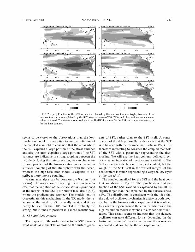
The coupled manifold for the SST and the heat con-tent are shown in Fig. 20. The panels show that thefraction of the SST variability explained by the HC isslightly larger than that explained by the surface stress,68%. The distribution is consistent with the idea thatthe delayed oscillator mechanism is active in both mod-els, but in the low-resolution experiment it is confinedto a narrow region around the equator, whereas in thehigh-resolution model it extends to a wider belt of lati-tudes. This result seems to indicate that the delayedoscillator can take different forms, depending on thelatitudinal extent of the channel where the waves aregenerated and coupled to the atmospheric field.

FIG. 20. (left) Fraction of the SST variance explained by the heat content and (right) fraction of theheat content variance explained by the SST. (top to bottom) T30, T106, and observations; annual meanvalues are used. The observations used were the HadISST dataset for the SST and the ocean reanalysisfor the heat content.


It is also interesting to note how the amount of SSTvariance explained by the U stress and the HC is dis-tributed in different areas. The SST variations seem tobe strongly linked to the HC in the east Pacific, devel-oping into a wide pattern into the central Pacific. Onthe other hand, the SST variations are strongly ex-plained by U-stress variations in the central Pacific. Themodels tend to misrepresent this behavior; the low-resolution model tends to have a really small fraction ofthe SST variance explained by the stress, whereas theSST variance is explained mostly by the HC variations.The high-resolution model realizes a better mix of thetwo mechanisms, and although it is still far from beingsatisfactory, it is closer to the observations.

6. Discussion

One of the most interesting results of this paper is theindication that the higher-resolution model is coupledto the atmosphere in wider region than the low-resolution model. The effect may appear counterintui-tive since the low-resolution model has a natural ten-dency to spread out the atmospheric information over awider oceanic area. However, the spreading may actu-ally be a negative factor in the simulation of how theocean and atmosphere interact. A low-resolution atmo-spheric model will spread the same information over alarge number of ocean grid boxes, resulting in an un-realistic uniformity of forcing over the ocean. The ex-amples of the tropical instability waves show how thelow-resolution atmospheric model is missing the inter-action with the ocean at the smaller scales and there-fore is not able to represent the consequent TIW-induced feedback to the ocean. The high resolution isexerting its impacts through small-scales effect like this,resulting in a better variability of wind forcing in theeast Pacific. Processes like these contribute to create adifferent basic state in the T106 from the T30. Thechange of basic state is visible in the mean SST (Fig. 3)and in the mean surface stress (Figs. 4 and 5). Thewinter wind stress in the T106 is more realistic than theT30 at the equator and it has a better geographicalextension, stopping short of the date line rather thanextending right to it as in the T30 case. The summerwind stress is also weaker at the equator and thereforecloser to the observed values. Probably, also as a con-sequence of the weaker winds, the SST in the westernPacific is warmer and the 29° area is larger in the T106and extends over a wider latitudinal extent. The coldtongue, however, is still extending too much west.

The Pacific can sustain a large variety of interannualocean and coupled modes (Jin 2001; Fedorov and Phi-lander 2000) and the basic state can select to emphasize

one or the other (Dewitte et al. 2007). Weaker winds atthe equator and a larger meridional scale have alsobeen connected with longer ENSO time scales (Kirt-man 1997; Capotondi et al. 2006), as the basic statesimulated by the T106 coupled model shows a morerealistic meridional profile of the zonal wind stressesthat is favorable to the slower modes. The change in thebasic state is affecting the mixing of the different modesof interannual variability as they were identified byFedorov and Philander (2000). The SST mode is limitedto the equator and does not involve much off-equatorvariability of the thermocline, whereas the thermoclinemode connected to the delayed oscillator shows off-equator variability. In practice the variability includesboth modes and so the changes in the basic state modifythe relative mix of the two. However, inspection of theheat content standard deviation (not shown) also showsthat there is more activity off the equator in the T106,rather than in the T30. The more prominent role of thedelayed oscillator mode can also be seen in Figs. 13 and14, which show how the T106 stays coupled longer thanthe T30, and in the coupled manifold (Figs. 19 and 20)that also indicates coupling over a wider area. The dif-ference between T106 and T30 can then be understoodas a more prominent role played by the delayed oscil-lator mode in the T106 due to the differences in basicstate between the two simulations.

7. Conclusions

This paper has shown that using a high horizontalresolution atmospheric component in a coupled modelis beneficial regarding the space–time characteristics ofthe tropical variability. The improvement is mostly vis-ible in the Pacific, but certain aspects of the surfaceatmospheric circulation in the Indian sector that is cru-cial for the simulation of the summer Indian monsoonare also improved. The comparison between the low-and high-resolution models shows that in the high-resolution model the delayed oscillator is at work in amore realistic set of parameters. The interaction be-tween ocean and atmosphere is realized in a wider lati-tudinal region and not confined in a narrow strip alongthe equator. The extension of more off-equatorial re-gions into the coupling allows the triggering of sloweroff-equatorial waves that allow slower time scales andshift the dominant Niño-3 variability toward longertime periods.

The introduction of high horizontal resolution hasother effects related to the introduction of smaller-scalemechanisms. The coastal upwelling along the SouthAmerican coast is improved, reducing the systematicerror in the mean SST in the east Pacific. Regions of


strong curl along the Mexican Pacific coast are visible inhigh-resolution satellite observations and are present inthe T106, but totally absent in the T30 and barelyhinted at in the reanalysis. They are probably linked tobetter resolved orographic features. Tropical instabilitywaves become coupled to the atmosphere, showing aclear signature pattern in the divergence field, as hasbeen discussed by Chelton (2005). The ocean compo-nent is producing tropical instability waves in bothmodels, but the atmosphere becomes sensitive to themonly in the high-resolution case. There is also someground to argue that the reanalysis is showing its limi-tation due to relatively low resolution used, and it isprobably time to produce a high-resolution atmo-spheric reanalysis datasets.

The coupled manifold approach allows the identifi-cation of the mechanisms of interannual variability inthe models and in the observations. Delayed oscillator-like mechanisms are the cause of the tropical Pacificinterannual variability in the models, but in the lowresolution model it is confined to a narrow region closeto the equator, yielding a faster period for the oscilla-tion. The results suggest that this is probably due to thefaster propagation of the waves in this area and to theweak coupling between U stress and SST. In the high-resolution model, the delayed oscillator involves awider latitudinal extent and the U stress is bettercoupled to the SST with a mix of mechanisms that isprobably closer to reality. It can also be speculated thatthe involvement of slower waves caused by the widerlatitudinal extent of the variations in the high-resolution model might lead to the spectral shift of thepeak of the variability toward longer time scales.

The increase of horizontal resolution therefore hasimpacts on a variety of phenomena, but it is far frombeing a “magic bullet” that fixes all the deficiencies ofthe models. In particular, the presence of a doubleITCZ does not seem to be affected by resolution and itcontinues to afflict the high-resolution simulation. Also,in the Indian Ocean the increase in resolution some-what negatively affects the variability in the east IndianOcean. The excessive penetration of the cold tongueand interannual variability too much in the west is alsonot affected by the change in resolution. The indication,however, is that improvements of the model can have abetter return if sufficient resolution is used.

Acknowledgments. This research was partially sup-ported by the Italy–USA Cooperation Program of theItalian Ministry of Environment and by the EU projectsENSEMBLES and DYNAMITE. It is a pleasure toacknowledge Dr. Ralph Milliff of CORA, Boulder, forkindly providing the QuikSCAT data and figure.

REFERENCES

Battisti, D. S., 1988: Dynamics and thermodynamics of a warmingevent in a coupled tropical atmosphere–ocean model. J. At-mos. Sci., 45, 2889–2919.

Bengtsson, L., M. Botzet, and M. Esch, 1995: Hurricane-type vor-tices in a general circulation model. Tellus, 47A, 175–196.

Boville, B., 1991: Sensitivity of simulated climate to model reso-lution. J. Climate, 4, 469–485.

Boyle, J., 1993: Sensitivity of dynamical quantities to horizontalresolution for a climate simulation using the ECMWF (cycle33) model. J. Climate, 6, 796–815.

Brankovic, C., and D. Gregory, 2001: Impact of horizontal reso-lution on seasonal integrations. Climate Dyn., 18, 123–143.

Capotondi, A., A. Wittenberg, and S. Masina, 2006: Spatial andtemporal structure of tropical Pacific interannual variabilityin 20th century coupled simulations. Ocean Modell., 15, 274–298.

Chelton, D. B., 2005: The impact of SST specification on ECMWFsurface wind stress fields in the eastern tropical Pacific. J.Climate, 18, 530–550.

——, and Coauthors, 2001: Observations of coupling between sur-face wind stress and sea surface temperature in the easterntropical Pacific. J. Climate, 14, 1479–1498.

——, M. Schlax, M. H. Freilich, and R. Milliff, 2004: Satellitemeasurements reveal persistent small-scale features in oceanwinds. Science, 303, 978–983.

Dewitte, B., C. Cibot, C. Périgaud, S.-I. An, and L. Terray, 2007:Interaction between near-annual and ENSO modes in aCGCM simulation: Role of the equatorial background meanstate. J. Climate, 20, 1035–1052.

Duffy, P. B., B. Govindasamy, J. P. Iorio, J. Milovich, K. R. Sper-ber, K. E. Taylor, M. F. Wehner, and S. L. Thompson, 2003:High-resolution simulations of global climate, part 1: Presentclimate. Climate Dyn., 21, 371–390.

Fedorov, A. V., and S. G. Philander, 2000: Is El Niño changing?Science, 288, 1997–2002.

Gualdi, S., A. Navarra, and H. von Storch, 1997: Tropical intrasea-sonal oscillation appearing in operational analyses and in afamily of general circulation models. J. Atmos. Sci., 54, 1185–1202.

——, E. Guilyardi, P. Delecluse, S. Masina, and A. Navarra,2003a: The role of the Indian Ocean in a coupled model.Climate Dyn., 20, 567–582.

——, A. Navarra, E. Guilyardi, and P. Delecluse, 2003b: Assess-ment of the tropical Indo-Pacific climate in the SINTEXCGCM. Ann. Geophys., 46, 1–5.

——, A. Alessandri, and A. Navarra, 2005: Impact of atmospherichorizontal resolution on El Niño Southern Oscillation fore-casts. Tellus, 57A, 357–374.

Guilyardi, E., P. Delecluse, S. Gualdi, and A. Navarra, 2003:Mechanism for ENSO phase change in a coupled GCM. J.Climate, 16, 1141–1158.

——, and Coauthors, 2004: Representing El Niño in coupledocean–atmosphere GCMs: The dominant role of the atmo-spheric component. J. Climate, 17, 4623–4629.

Hashizume, H., S.-P. Xie, W. T. Liu, and K. Takeuchi, 2001: Localand remote atmospheric response to tropical instabilitywaves: A global view from space. J. Geophys. Res., 106,10 173–10 186.

Jin, F.-F., 2001: Low-frequency modes of tropical ocean dynamics.J. Climate, 14, 3874–3881.

Junge, M. M., R. Blender, K. Fraedrich, V. Gayler, U. Luksch,


and F. Lunkeit, 2005: A world without Greenland: Impactson the Northern Hemisphere winter circulation in low- andhigh-resolution models. Climate Dyn., 24, 297–307.

Kalnay, E., and Coauthors, 1996: The NCEP/NCAR 40-Year Re-analysis Project. Bull. Amer. Meteor. Soc., 77, 437–471.

Kirtman, B., 1997: Oceanic Rossby wave dynamics and the ENSOperiod in a coupled model. J. Climate, 10, 1690–1704.

Kistler, R., and Coauthors, 2001: The NCEP–NCAR 50-Year Re-analysis: Monthly means CD-ROM and documentation. Bull.Amer. Meteor. Soc., 82, 247–267.

Kobayashi, C., and M. Sugi, 2004: Impact of horizontal resolutionon the simulation of the Asian summer monsoon and tropicalcyclones in the JMA global model. Climate Dyn., 23, 165–176.

Liu, W. T., X. Xie, P. S. Polito, S.-P. Xie, and H. Hashizume, 2000:Atmospheric manifestation of tropical instability waves ob-served by QuikSCAT and Tropical Rain Measuring Mission.Geophys. Res. Lett., 27, 2545–2548.

Luo, J.-J., S. Masson, S. Behera, P. Delecluse, S. Gualdi, A. Na-varra, and T. Yamagata, 2003: South Pacific origin of thedecadal ENSO-like variation as simulated by a coupledGCM. Geophys. Res. Lett., 30, 2250–2258.

——, ——, E. Roeckner, G. Madec, and T. Yamagata, 2005: Re-ducing climatology bias in an ocean–atmosphere CGCM withimproved coupling physics. J. Climate, 18, 2344–2360.

Manabe, S., J. Smagorinsky, J. L. Holloway Jr., and H. M. Stone,1970: Simulated climatology of a general circulation modelwith a hydrologic cycle. III: Effects of increased horizontalcomputational resolution. Mon. Wea. Rev., 98, 175–212.

Masina, S., N. Pinardi, and A. Navarra, 2001: A global oceantemperature and altimeter data assimilation system for stud-ies of climate variability. Climate Dyn., 17, 687–700.

——, P. Di Pietro, and A. Navarra, 2004: Interannual-to-decadalvariability of the North Atlantic from an ocean data assimi-lation system. Climate Dyn., 23, 531–546.

May, W., 2001: The impact of horizontal resolution on the simu-lation of seasonal climate in the Atlantic/European area forpresent and future times. Climate Res., 16, 203–223.

——, 2003: The Indian summer monsoon and its sensitivity to themean SSTs: Simulations with the ECHAM4 AGCM at T106horizontal resolution. J. Meteor. Soc. Japan, 81, 57–83.

——, and E. Roeckner, 2001: A time-slice experiment with theECHAM4 AGCM at high resolution: The impact of horizon-tal resolution on annual mean climate change. Climate Dyn.,17, 407–420.

McCreary, J. P., H. S. Lee, and D. B. Enfield, 1989: The responseof the coastal ocean to strong offshore winds: With applica-

tion to circulations in the gulfs of Tehuantepec and Papa-gayo. J. Mar. Res., 47, 81–109.

Navarra, A., 2003: Preface: The SINTEX Project. Ann. Geophys.,46, V–IX.

——, and J. Tribbia, 2005: The coupled manifold. J. Atmos. Sci.,62, 310–330.

Pope, V., and R. Stratton, 2002: The processes governing hori-zontal resolution sensitivity in a climate model. Climate Dyn.,19, 211–236.

Rayner, N. A., D. E. Parker, E. B. Horton, C. K. Folland, L. V.Alexander, D. P. Rowell, E. C. Kent, and A. Kaplan, 2003:Global analyses of SST, sea ice, and night marine air tem-perature since the late nineteenth century. J. Geophys. Res.,108, 4407, doi:10.1029/2002JD002670.

Roeckner, E., and Coauthors, 1996: The atmospheric general cir-culation model ECHAM-4: Model description and simula-tion of present-day climate. Max-Planck-Institut für Meteo-rologie Rep. 218, 90 pp.

Schopf, P., and M. J. Suarez, 1990: Ocean wave dynamics and thetime scale of ENSO. J. Phys. Oceanogr., 20, 629–645.

Sperber, K., S. Hameed, G. L. Potter, and J. S. Boyle, 1994: Simu-lation of the northern summer monsoon in the ECMWFmodel: Sensitivity to horizontal resolution. Mon. Wea. Rev.,122, 2461–2481.

Stephenson, D. B., F. Chauvin, and J.-F. Royer, 1998: Simulationof the Asian summer monsoon and its dependence on modelhorizontal resolution. J. Meteor. Soc. Japan, 76, 237–265.

Stratton, R. A., 1999: A high resolution AMIP integration usingthe Hadley Centre model HadAM2b. Climate Dyn., 15, 9–28.

Suarez, M. J., and P. S. Schopf, 1988: A delayed action oscillatorfor ENSO. J. Atmos. Sci., 45, 3283–3287.

Tibaldi, S., T. N. Palmer, C. Brankovic, and U. Cubasch, 1990:Extended-range predictions with ECMWF models: Influenceof horizontal resolution on systematic error and forecast skill.Quart. J. Roy. Meteor. Soc., 116, 835–866.

Welch, P., 1967: The use of fast Fourier transform for the estima-tion of power spectra: A method based on time averagingover short, modified periodograms. IEEE Trans. Audio Elec-troacoust., 15, 70–73.

Wild, M., P. Calanca, S. C. Scherrer, and A. Ohmura, 2003: Ef-fects of polar ice sheets on global sea level in high-resolution.J. Geophys. Res., 108, 4165, doi:10.1029/2002JD002451.

Williamson, D. L., J. T. Kiehl, and J. J. Hack, 1995: Climate sen-sitivity of the NCAR Community Climate Model (CCM2) tohorizontal resolution. Climate Dyn., 11, 377–397.

Wittenberg, A. T., 2004: Extended wind stress analyses for ENSO.J. Climate, 17, 2526–2540.


Documents

Atmospheric Horizontal Resolution Affects Tropical Climate ... · in the T30 model is moderated in the T106 as it shifts to a longer time scale. At high resolution, new processes