Asynchronous Variational Contact Mechanics

E. Vougaa,∗, D. Harmona, R. Tamstorfb, E. Grinspuna

aComputer Science Department, Columbia University, New York, New York 10027bWalt Disney Animation Studios, Burbank, California 91521

Abstract

An asynchronous, variational method for simulating elastica in complex contact and impact scenariosis developed. Asynchronous Variational Integrators [1] (AVIs) are extended to handle contact forcesby associating different time steps to forces instead of to spatial elements. By discretizing a barrierpotential by an infinite sum of nested quadratic potentials, these extended AVIs are used to resolve con-tact while obeying momentum- and energy-conservation laws. A series of two- and three-dimensionalexamples illustrate the robustness and good energy behavior of the method.

Keywords: contact, impact, variational integrators

1. Introduction

Variational integrators (VIs) [2, 3, 4] are a general class of time integration methods for Hamiltoniansystems whose construction guarantees certain properties highly desirable of numerical simulations.Instead of directly discretizing the smooth equations of motion of a system, the variational approachinstead discretizes the system’s action integral. By analogy to Hamilton’s least action principle, adiscrete action can be formed, and discrete Euler-Lagrange equations derived by examining pathswhich extremize it. From the Euler-Lagrange equations, discrete equations of motion are readilyrecovered. As a consequence of this special construction, VIs are guaranteed to satisfy a discreteformulation of Noether’s Theorem [5], and as a special case conserve linear and angular momentum.VIs are automatically symplectic [6]; while they do not necessarily conserve energy, conservation of thesymplectic form assures no-drift conservation of energy over exponentially many time steps [6].

Given the many advantages of VIs, it is natural to apply them to the handling of contact and impact,a long-studied and challenging problem in physical simulation. Unfortunately, a naıve application of acontact algorithm to a variational integrator is not guaranteed to preserve the variational structure ofthe time integration method, and in practice one observes that the good energy behavior is lost. Forthis reason, a few recent works have explored structure-preserving approaches for contact mechanics [7,8, 9, 10]. Common to all these approaches is a synchronous treatment of global time, in which theentire configuration is advanced from one intant in time to the next. While synchronous integrationis attractive for its simplicity, it has the drawback that a spatially-localized stiff mode—such as thatassociated to a localized contact—can force the global configuration to advance at fine time steps.

Indeed, mechanical systems are almost never uniformly stiff. Different potentials have differentstable time step requirements, and even for identical potentials this requirement depends on element

∗Corresponding author

Preprint submitted to Elsevier March 16, 2011

size, since finer elements can support higher-energy modes than coarser elements. Any global timeintegration scheme cannot take advantage of this variability, and instead must integrate the entiresystem at the globally stiffest time step.

Suppose the system can be partitioned into elements such that each force acts entirely within oneelement. Then asynchronous variational integrators (AVIs) [1] generalize VIs by allowing each elementto have its own, independent time step. Coarser elements can then be assigned a slower “clock,” andfiner elements a faster one. Asynchrony avoids the undesirable situation in which a small number of veryfine elements degrade overall performance. AVIs retain all of the properties of variational integratorsmentioned above, except for discrete symplecticity. However, AVIs instead preserve an analogousdiscrete multisymplectic form, and it has been shown experimentally that preservation of this formlikely induces the same long-time good energy behavior that characterize symplectic integrators [1].

To our knowledge, this work is the first to consider an asynchronous, variational treatment of contactshown to retain multisymplecity. Rangarajan et al. [11] suggest AVIs for simulating penetration of asoft hyperelastic material by rigid bodies, and propose handling contact by reflecting momentum at theend of any elemental time step during which contact occurred. This method was observed to dissipateenergy during contact events; the amount of drift can be controlled by appropriately decreasing the timesteps of elements involved in contact. We are also aware that Ryckman and Lew [12] are concurrentlyinvestigating extending the AVI framework to incorporate contact response.

The starting point for this approach is the selection of the penalty method as a model for contact [13,14]. For each pair of elements in the system, a potential is added that is (piecewise) quadratic in the gapfunction measuring the separation distance between the two elements. This potential vanishes whenelements are sufficiently far apart, and increases with increasing interpenetration, so that approachingelements feel a force that resists impact. This approach suffers two limitations, however. Firstly, thesecontact potentials are fundamentally nonlocal phenomena: for every pair of elements that might comeinto contact during the course of the simulation, a potential coupling the two must be added. As willbe shown, the fact that contact potentials cannot be expressed as the integration over the materialdomain of an energy density depending only on a neighborhood of the domain will present a technicalobstruction to the original formulation of AVIs, but fortunately one that can be overcome by a naturalgeneralization.

Secondly, penalty forces have a well-studied performance-robustness tradeoff [15]: adding a half-quadratic potential requires choosing an arbitrary stiffness parameter, and for any stiffness chosenfor the penalty potential, two approaching elements will interpenetrate some distance, and in theworst case tunnel completely through each other. Moreover, the stable time step of the penalty forcedecreases as stiffness increases, so choosing a very stiff penalty potential is untenable as a solutionto excessive penetration or tunneling. In practice, users of the method must determine an adequatepenalty stiffness by iterated tweaking of parameters, until the simulation completes without collisionartifacts. An appealing modification of the penalty approach replaces the quadratic potential witha nonlinear barrier potential [16] that diverges as the configuration approaches contact. Because thebarrier diverges, its stiffness is unbounded, necessitating a time-adaptive time stepping method. Thiswork presents a discrete analogue of the barrier potential—an infinite sequence of discrete penaltylayers—that in effect enables AVIs to serve as adaptive integrators.

This paper

• extends the construction of AVIs so that a discretization into disjoint elements is no longernecessary, by associating a clock to each force instead of to each element;

• demonstrates that this generalization does not destroy the desirable integration properties guar-

2

anteed by the variational paradigm, most importantly the conservation of the discrete multisym-plectic form;

• leverages this extension to equip the AVI framework with a contact model. The proposed barriermethod uses a divergent sequence of quadratic potentials that guarantees non-penetration andretains the asynchrony or conservation properties of AVIs;

• presents numerical evidence to support the claim that by retaining the symplectic structureof the smooth system, simulations of thin shells undergoing complex (self-)interactions havedemonstrably good long-time energy and momentum behavior;

• describes simple extensions to the contact model to allow for controlled, dissipative phenom-ena, such as a coefficient of restitution and kinetic friction. Although there is not yet theoryexplaining the energy behavior of dissipative simulations run under a variational integrator, em-pirical evidence is presented to show that the proposed method produces smooth, controlled, andqualitatively correct energy decay.

This paper complements the publication [17], which provides a detailed description of the softwareimplementation using kinetic data structures [18]. For completeness, Section 6 briefly introduces theseconcepts.

2. Related Work

The simplest contact models for finite element simulation follow the early analytical work ofHertz [19] in assuming frictionless contact of planar (or nearly planar) surfaces with small strain.In this regime, several approaches have been explored to arrive at a weak formulation of contact;for a high-level survey of these approaches, see for example the overview by Belytschko et al. [20] orWriggers [21]. The first of these are the use of penalty forces, described for instance by Oden [22] andKikuchi and Oden [23]. The penalty approach results in a contact force proportional to an arbitrarypenalty stiffness parameter and to the rate of interpenetration, or in more general formulations to anarbitrary function of rate of interpenetration and interpenetration depth; Belytschko and Neal [15]discuss the choosing of this parameter in Section 8. Recent work by Belytschko et al. [24] uses movingleast squares to construct an implicit smooth contact surface, from which the interpenetration distanceis evaluated. Peric and Owen [25] describe how to equip penalty forces with a Coulomb friction model.

Seeking to exactly enforce non-penetration along the contact surface leads to generalizations ofthe method of Lagrange multipliers. Hughes et al. [26] and Nour-Omid and Wriggers [27] providean overview of this approach in the context of contact response. Such contraint enforcement canbe viewed as a penalty force in the limit of infinite stiffness, impossible to attain in practice sincethe system becomes ill-conditioned. Taylor and Papadopoulos [28] considers persistent contact byextending Newmark to treat jump conditions in kinematic fields, thus reducing undesirable oscillatorymodes. However, the effects of these modifications on numerical dissipation and long-time energybehavior is not considered.

The Augmented Lagragian method blends the penalty and Lagrange multiplier approaches, andcombines the advantages of both: unlike for pure penalty forces, convergence to the exact interpene-tration constraint does not require taking the penalty stiffness to infinity, and the Lagrange multipliersolve tends to be well-conditioned. Bertsekas [29] gives a mathematical overview of the augmentedLagrangian method, and Wriggers et al. [30] and Simo and Laursen [31] expand on its application tocontact problems in finite elements.

3

Non-smooth contact requires special consideration, since in the non-smooth regime there is nostraightforward way of defining a contact normal or penetration distance. Simo et al. [32] discretizethe contact surface into segments over which they assume constant contact pressure; this formulationallows them to handle non-node-to-node contact using a perturbed Lagrangian. Kane et al. [33] applynon-smooth analysis to resolve contact constraints between sharp objects. Pandolfi et al. [10] extend thework of Kane et al. by describing a variational model for non-smooth contact with friction. Cirak andWest [34] decompose contact resolution into an impenetrability-enforcement and momentum-transferstep, thereby exactly enforcing non-interpenetration while nearly conserving momentum and energy.

Several authors have explored a structure-preserving approach to solving the contact problem.Barth et al. [7] consider an adaptive-step-size algorithm that preserves the time-reversible symmetry ofthe RATTLE algorithm, and demonstrate an application to an elastic rod interacting with a Lennard-Jones potential. Kane et al. [8] show that the Newmark method, for all parameters, is variational,and construct two two-step dissipative integrators that yield good energy decay. Laursen and Love [9],by taking into account velocity discontinuities that occur at contact interfaces, develop a momentum-and energy-preserving method for simulating frictionless contact. This paper shares with these lastapproaches the viewpoint that structured integration, with its associated conservation guarantees, isan invaluable tool for accurately simulating dynamic systems with contact.

Although several previous approaches are also adaptive, the algorithm described in this paper isthe first structured integrator for contact mechanics that achieves time adaptivity using asynchrony.This novel approach guarantees the robustness of the proposed integrator, without compromising thegood properties of structured integration.

3. Variational Integrators

This section presents a background on variational integration and symplectic structure [6, 4, 5].Let γ(t) be a piecewise-regular trajectory through configuration space Q, and γ(t) = d

dtγ(t) be theconfigurational velocity at time t. For simplicity, assume that the kinetic energy of the system T de-pends only on configurational velocity, and that the potential energy V depends only on configurationalposition, so that the Lagrangian L at time t may be written as

L(q, q) = T (q)− V (q). (1)

Then given the configuration of the system q0 at time t0 and qf at tf , Hamilton’s principle [35]states that the trajectory of the system γ(t) joining γ(t0) = q0 and γ(tf ) = qf is a stationary point ofthe action functional

S(γ) =

∫ tf

t0

L [γ(t), γ(t)] dt

with respect to taking variations δγ of γ which leave γ fixed at the endpoints t0, tf . In other words,γ satisfies

dS(γ) · δγ = 0. (2)

4

Integrating by parts, and using that δγ vanishes at t0 and t1,

dS(γ) · δγ =

∫ tf

t0

(∂L

∂q(γ, γ) · δγ +

∂L

∂q(γ, γ) · δγ

)dt =

∫ tf

t0

(−∂V∂q

(γ)− ∂2T

∂q2(γ)γ

)· δγ dt = 0.

Since this equality must hold for all variations δγ that fix γ’s endpoints,

∂V

∂q(γ) +

d

dt

(∂T

∂q(γ)

)= 0, (3)

the Euler-Lagrange equation of the system. This equation is a second-order ordinary differentialequation, and so has a unique solution γ given two initial values γ(t0) and γ(t0).

3.1. Symplecticity

The flow Θs : [γ(t), γ(t)] 7→ [γ(t+ s), γ(t+ s)] induced by (3) has many structure-preserving prop-erties; in particular it is momentum-preserving, energy-preserving, and symplectic [36]. To derive thislast property, for the remainder of this section the space of trajectories is restricted to those that satisfythe Euler-Lagrange equations. For such trajectories, if the requirement that δγ fix the endpoints of γis relaxed, then the boundary terms of the integration by parts are no longer 0 and

dS(γ) · δγ =∂T

∂q[πq(q, q)] · δγ

∣∣∣∣tft0

, (4)

where πq is projection onto the second factor.Since initial conditions (q, q) are in bijection with trajectories satisfying the Euler-Lagrange equa-

tion, such trajectories γ can be uniquely parametrized by initial conditions [γ(t0), γ(t0)]. For theremainder of this section variations δγ are also restricted to first variations: those variations inwhose direction γ continues to satisfy the Euler-Lagrange equations. These are also parametrizedby variations of the initial conditions, (δq, δq). For conciseness of notation, the change of variablesν(t) = (γ(t), γ(t)) and δν(t) = [δγ(t), δγ(t)] can be used; using this notation the above two facts can berewritten as ν(t) = Θt−t0ν(t0) and δν(t) = Θt−t0∗δν(t0). The action (1), a functional on trajectoriesγ, can also be rewritten as a function Si of the intial conditions,

Si(q, q) =

∫ tf−t0

0

L [Θt(q, q)] dt,

so that

dS(γ) · δγ = dSi [ν(t0)] · δν(t0).

5

Substituting all of these expressions into (4),

dSi [ν(t0)] · δν(t0) =

(∂T

∂q◦ πq

)[Θt−t0ν(t0)] · δγ(t)

∣∣∣∣tft0

=

(∂T

∂q◦ πq

)[Θt−t0ν(t0)] dq · δν(t)

∣∣∣∣tft0

=

(∂T

∂q◦ πq

)[Θt−t0ν(t0)] dq ·Θt−t0∗δν(t0)

∣∣∣∣tft0

= (Θtf−t0∗θL − θL)ν(t0) · δν(t0),

where θL is the one-form(∂T∂q ◦ πq

)dq. Since dSi is exact,

d2Si = 0 = Θtf−t0∗dθL − dθL,

so since t0 and tf are arbitrary, Θ∗sdθL = dθL for arbitrary times s, and Θ preserves the so-calledsymplectic form dθL.

3.2. Discretization

Discrete mechanics [37, 2, 38, 39, 4, 6] describes a discretization of Hamilton’s principle, yielding anumerical integrator that shares many of the structure-preserving properties of the continuous flow Θs.Consider a discretization of the trajectory γ : [t0, tf ]→ Q by a piecewise linear trajectory interpolatingn points q = {q0, q1, . . . qn−1}, with q0 = γ(t0) and qn−1 = γ(tf ), where the discrete velocity qi+1/2 onthe segment between qi and qi+1 is

qi+1/2 =qi+1 − qi

h, h =

tf − t0n

.

An analogue of (3) in this discrete setting is needed. To that end, a discrete Lagrangian

Ld(qa, qb) = T

(qb − qah

)− V (qb) (5)

can be formulated, as well as a discrete action

Sd(q) =

n−2∑i=0

hLd(qi, qi+1). (6)

Motivated by (2), a discrete Hamilton’s principle can be imposed:

dSd(q) · δq = 0

for all variations δq = {δq0, δq1, . . . , δqn−1} that fix q at its endpoints, i.e., with δq0 = δqn−1 = 0. Forease of notation, the kinetic and potential energy terms in (5) can be written to depend on (qa, qb),

6

two points of phase space consecutive in time, instead of (q, q):

Td(qa, qb) = T

(qb − qah

)T ′d(qa, qb) =

∂T

∂q

(qb − qah

)Vd(qa, qb) = V (qb) V ′d(qa, qb) =

∂V

∂q(qb).

Then

dSd(q) · δq =

n−2∑i=0

h (D1Ld(qi, qi+1) · δqi +D2Ld(qi, qi+1) · δqi+1)

=

n−2∑i=0

h

(− 1

hT ′d(qi, qi+1) · δqi +

1

hT ′d(qi, qi+1) · δqi+1 −

∂V

∂q(qi+1) · δqi+1

)= T ′d(qn−2, qn−1) · δqn−1 − T ′d(q0, q1) · δq0 − h

∂V

∂q(qn−1) · δqn−1

+

n−2∑i=1

(T ′d(qi−1, qi)− T ′d(qi, qi+1)− h∂V

∂q(qi)

)· δqi

=

n−2∑i=1

(T ′d(qi−1, qi)− T ′d(qi, qi+1)− h∂V

∂q(qi)

)· δqi = 0.

Since δqi is unconstrained for 1 ≤ i ≤ n− 2,

∂T

∂q(qi+1/2)− ∂T

∂q(qi−1/2) = −h∂V

∂q(qi), i = 1, . . . , n− 2, (7)

the discrete Euler-Langrange equations of the system.Unlike in the continuous settings, the discrete Euler-Lagrange equations do not always have a

unique solution given initial values q0 and q1. Therefore in all that follows it is assumed that Td andVd are of a form so that (7) gives a unique qi+1 given qi and qi−1—this assumption always holds, forinstance, in the typical case where Td is quadratic in q. Then the discrete Euler-Lagrange equationsgive a well-defined discrete flow

F : (qi−1, qi) 7→ (qi, qi+1),

which recovers the entire trajectory from initial conditions, in perfect analogy to the continuous setting.

3.3. Symplecticity of the Discrete Flow

By analogy to the continuous setting, it is desired that F preserve a symplectic form, just as dθLis preserved by Θ. As in the continuous setting, trajectories q are restricted to those that satisfythe discrete Euler-Lagrange equations, and variations to first variations (and the condition that thesevariations vanish at the endpoints is lifted), yielding

dSd(q) · δq = T ′d(qn−2, qn−1) · δqn−1 − T ′d(q0, q1) · δq0 − h∂V

∂q(qn−1) · δqn−1.

7

F k denotes the discrete flow F composed with itself k times, or k “steps” of F . Again, all q satisfying(7) can be parametrized by initial conditions ν0 = (q0, q1), and first variations by δν0 = (δq0, δq1), sothat the discrete action can be rewritten as

Sid(ν0) =

n−2∑i=0

hLd(Fiν0).

Putting together all of the pieces,

dSid(ν0) · δν0 = dSd(q) · δq

= T ′d(qn−2, qn−1) · δqn−1 − T ′d(q0, q1) · δq0 − h∂V

∂q(qn−1) · δqn−1

=

(T ′d(qa, qb)− h

∂V

∂q(qb)

)dqb · (δqn−2, δqn−1)

∣∣∣qa=qn−2, qb=qn−1

=[T ′d(F

n−2ν0)− hV ′(Fn−2ν0)]dqb · Fn−2∗δν0 − T ′d(ν0)dqa · δν0

= θ+Fn−2ν0· Fn−2∗δν0 + θ−ν0 · δν0

=(Fn−2

∗θ+)ν0· δν0 + θ−ν0 · δν0.

for the indicated two-forms θ+ and θ−. Since d(hLd) = θ+ + θ−, d2(hLd) = 0 = dθ+ + dθ−. Moreoverthe initial conditions ν0 are arbitrary, hence

d2Sid = 0 =(Fn−2

)∗dθ+ + dθ− = −

(Fn−2

)∗dθ− + dθ−,

so

dθ− =(Fn−2

)∗dθ−.

Since n is arbitrary, the discrete flow F preserves the symplectic form dθ−. Using backwards erroranalysis, it can be shown that this geometric property guarantees that integrating with F introducesno energy drift for a number of steps exponential in h [6], a highly desirable property when simulatingmolecular dynamic or other Hamiltonian systems whose qualitative behavior is substantially affectedby errors in energy.

4. Asynchronous Variational Integrators

In Section 3.2 an action functional (6) was formulated as the integration of a single discrete La-grangian over a single time step size h. Such a construction is cumbersome when modeling multiplepotentials of varying stiffnesses acting on different parts of the system: to prevent instability one mustintegrate the entire system at the resolution of the stiffest force. Asynchronous variational integrators(AVIs), introduced by Lew et al. [1], are a family of numerical integrators, derived from a discreteHamilton’s principle, that support integrating potentials at different time steps. Their formulationassumes a spatial partition, with each potential depending only on the configuration of a single ele-ment; in this exposition, the general arguments set forth by Lew et al. are followed, but the notationand derivation departs from their work as necessary to support potentials with arbitrary, possiblynon-disjoint spatial stencil.

8

Let {V i} be potentials with time steps hi. Each potential V i is concerned with certain moments intime—namely, integer multiples of hi—and these moments are inconsistent across different potentials.Time is therefore subdivided in a way compatible with all potentials: for a τ -length interval of time,the set Ξ(τ) is defined by

Ξ(τ) =⋃V i

bτ/hic⋃j=0

jhi.

That is, Ξ(τ) is the set of all integer multiples less than τ of all time steps. Ξ can be ordered, and inparticular let ξ(i) be the (i+ 1)-st least element of Ξ. For ease of notation, also let ωi(j) = ξ−1(jhi);that is, ω converts the jth timestep of potential i into a global time index.

If n is the cardinality of Ξ, a trajectory of duration τ is then discretized by linearly interpolatingintermediate configurations q0, q1, . . . , qn−1, where qi is the configuration of the system at time ξ(i).Velocity is discretized as qk+1/2 = qk+1−qk

ξ(k+1)−ξ(k) on the segment of the trajectory between qk and qk+1.

A global action functional of these trajectories is needed, and can be constructed in the natural way:

Sg(q) =

n−2∑j=0

[ξ(j + 1)− ξ(j)]Td [qj , qj+1, ξ(j), ξ(j + 1)]−∑V i

bτ/hic∑j=1

hiV i(qωi(j)),

where, for T (q) the kinetic energy of the entire configuration, Td(qa, qb, ta, tb) = T(qb−qatb−ta

). For use in

the following, also let T ′d(qa, qb, ta, tb) = ∂T∂q

(qb−qatb−ta

).

No attempt has been made to define a Lagrangian pairing the kinetic and potential energy terms;it will be seen that an action defined in this way still leads to a multisymplectic numeric integrator.To this end, Hamilton’s principle dSg(q) · δq = 0 is imposed for variations δq = {δq0, . . . , δqn−1} withδq0 = δqn−1 = 0. Then Sg can be rewritten as

Sg(q) =

n−2∑j=0

[ξ(j + 1)− ξ(j)]Td [qj , qj+1, ξ(j), ξ(j + 1)]−n−1∑j=1

∑hi|ξ(j)

hiV i(qj), (8)

9

where the notation hi|ξ(j) is abused to mean “all indices i for which hi evenly divides ξ(j),” so that

dSg(q) · δq =

n−2∑j=0

T ′d [qj , qj+1, ξ(j), ξ(j + 1)] · (δqj+1 − δqj)−n−1∑j=1

∑hi|ξ(j)

hi∂Vi∂q

(qj) · δqj

= T ′d [qn−2, qn−1, ξ(n− 2), ξ(n− 1)] · δqn−1 − T ′d [q0, q1, ξ(0), ξ(1)] · δq0

−∑

hi|ξ(n−1)

hi∂V i

∂q(qn−1) · δqn−1

+

n−2∑j=1

T ′d [qj−1, qj , ξ(j − 1), ξ(j)]− T ′d [qj , qj+1, ξ(j), ξ(j + 1)]−∑hi|ξ(j)

hi∂V i

∂q(qj)

· δqj=

n−2∑j=1

T ′d [qj−1, qj , ξ(j − 1), ξ(j)]− T ′d [qj , qj+1, ξ(j), ξ(j + 1)]−∑hi|ξ(j)

hi∂V i

∂q(qj)

· δqj .The Euler-Lagrange equations are then

∂T

∂q(qk+1/2)− ∂T

∂q(qk−1/2) = −

∑hi|ξ(k)

hi∂V i

∂qi(qk), (9)

These equations are similar to those derived for synchronous variational integrators (7), except thatonly a subset of potentials V id contribute during each time step. As in the synchronous case, if, as istypical, Td(q) is quadratic in q, the system (9) gives rise to an explicit numerical integrator that isparticularly easy to implement in practice. Algorithm 1 gives pseudocode for such integration whenTd = qTMq for a mass matrix M; Lew et al. [36] discuss the algorithm in greater detail.

4.1. Multisymplecticity

The right hand side of (9) depends on ξ(k), and so unlike (7), the Euler-Lagrange equations for AVIsare time dependent, and do not give rise to a uniform update rule F (qi−1, qi) 7→ (qi, qi+1). Instead,consider the total, time-dependent flow F k(q0, qi) 7→ (qk, qk+1). Once again, trajectories satisfying(9) are parametrized by ν0 = (q0, q1), and first variations by δν0 = (δq0, δq1). By restricting to suchtrajectories and variations, the action (8) can be rewritten as

SiAVI =

n−2∑j=0

[ξ(j + 1)− ξ(j)]Td(F j(ν0), ξ(j), ξ(j + 1)

)−∑V i

bτ/hic−1∑j=0

hiV id (Fωi(j+1)(ν0)).

10

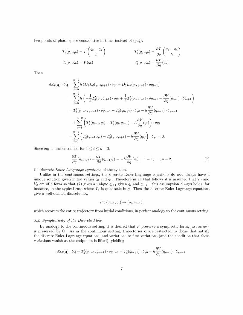
Algorithm 1 An algorithm for integrating the trajectory given by the AVI Euler-Lagrange equations(9) adapted from Lew et al. [36]

Let events be (potential, time step, time) triplets E = (V, h, t).Denote by qV the configuration subspace on which V depends.Let PQ be a priority queue of events, sorted by event times E.t.Tg ← 0 {Tg maintains the value of the simulation clock}q ← q0 {Set up initial conditions}q ← q0for all Vi doEi ← (Vi, h

i, hi) {Add all potentials to the queue as events}PQ.push(Ei)

end forloop

(V, h, t)← PQ.popq ← q + (t− Tg)qqV ← qV − hM−1V

∂V∂qV{Update only those elements affected by this event.}

PQ.push(V, h, t+ h) {Return the event to the queue, with a new, later time}Tg ← t {Update the simulation clock}

end loop

Then, for V id′(qa, qb) = ∂V i

∂q (q),

dSiAVI(ν) · δν = dSg(q) · δq= T ′d [qn−2, qn−1, ξ(n− 2), ξ(n− 1)] · δqn−1 − T ′d [q0, q1, ξ(0), ξ(1)] · δq0

−∑V i

∑hi|ξ(n−1)

hi∂V i

∂qi(qn−1) · δqn−1

= T ′d

[Fn−2(ν0), ξ(n− 2), ξ(n− 1)

]· δqn−1 − T ′d [ν0, ξ(0), ξ(1)] · δq0

−∑V i

∑hi|ξ(n−1)

hiV id′[Fn−2(ν0)

]· δqn−1

= θ−ν0 · δν0 + θ+Fn−2ν0

· Fn−2∗δν0

= (θ− + Fn−2∗θ+)ν0 · δν0

for one-forms θ− and θ+. Once again

0 = d2SiAVI = dθ− + Fn−2∗dθ+, (10)

but unlike when the action was a sum of Lagrangians, from the multisymplectic form formula (10)there is no way of relating dθ− to dθ+, and thus discrete symplectic structure preservation is notrecovered. Nevertheless, Lew et al. [1] conjecture that this multisymplectic structure leads to the goodenergy behavior observed for AVIs.

11

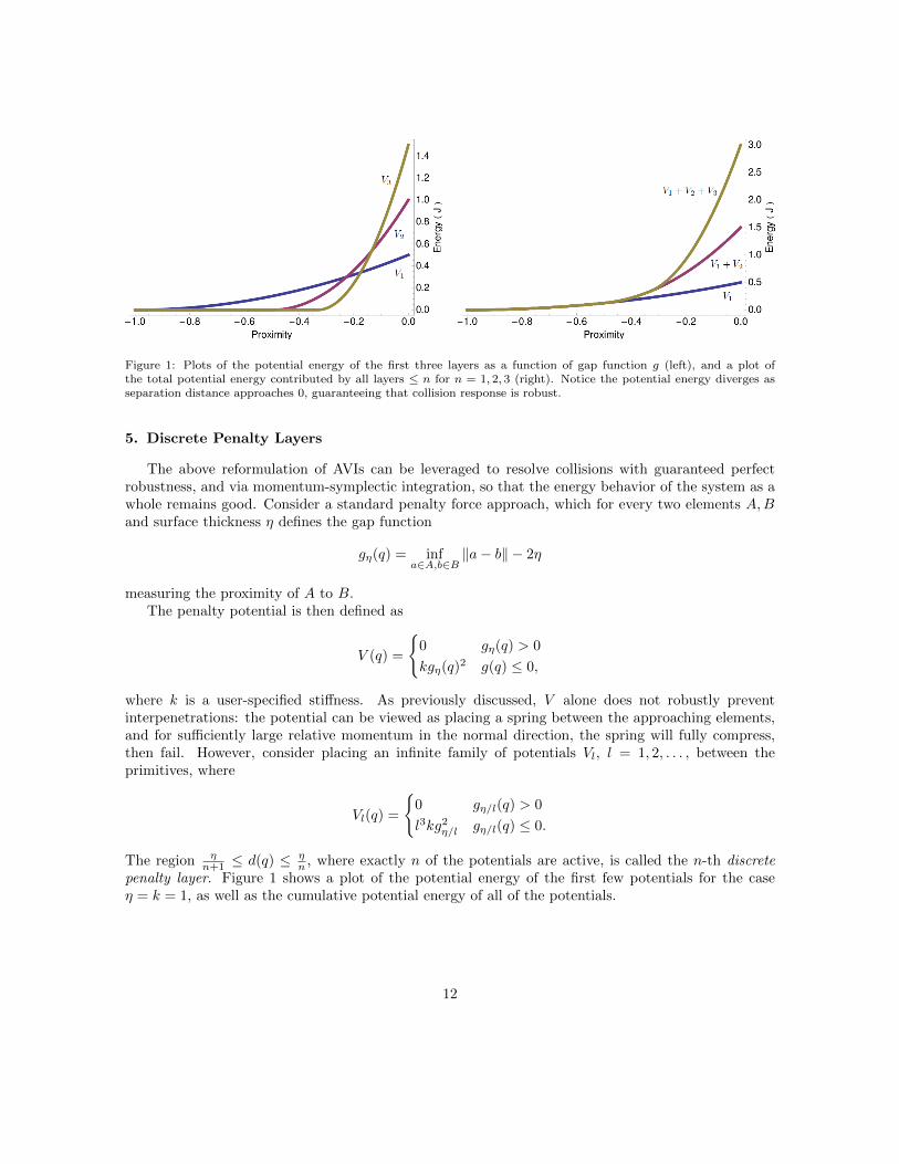
Figure 1: Plots of the potential energy of the first three layers as a function of gap function g (left), and a plot ofthe total potential energy contributed by all layers ≤ n for n = 1, 2, 3 (right). Notice the potential energy diverges asseparation distance approaches 0, guaranteeing that collision response is robust.

5. Discrete Penalty Layers

The above reformulation of AVIs can be leveraged to resolve collisions with guaranteed perfectrobustness, and via momentum-symplectic integration, so that the energy behavior of the system as awhole remains good. Consider a standard penalty force approach, which for every two elements A,Band surface thickness η defines the gap function

gη(q) = infa∈A,b∈B

‖a− b‖ − 2η

measuring the proximity of A to B.The penalty potential is then defined as

V (q) =

{0 gη(q) > 0

kgη(q)2 g(q) ≤ 0,

where k is a user-specified stiffness. As previously discussed, V alone does not robustly preventinterpenetrations: the potential can be viewed as placing a spring between the approaching elements,and for sufficiently large relative momentum in the normal direction, the spring will fully compress,then fail. However, consider placing an infinite family of potentials Vl, l = 1, 2, . . . , between theprimitives, where

Vl(q) =

{0 gη/l(q) > 0

l3kg2η/l gη/l(q) ≤ 0.

The region ηn+1 ≤ d(q) ≤ η

n , where exactly n of the potentials are active, is called the n-th discretepenalty layer. Figure 1 shows a plot of the potential energy of the first few potentials for the caseη = k = 1, as well as the cumulative potential energy of all of the potentials.

12

The total potential energy of the springs when fully compressed is

∞∑l=1

l3k4(ηl

)2= 4kη2

∞∑l=1

l,

which diverges. The infinite array of potentials is guaranteed to stop all collisions. This guaranteein no way depends on the chosen stiffness k: although performance and trajectory will vary with thechoice of stiffness, unlike for penalty forces the stiffness does not affect the guarantee. The method isalways guaranteed to be robust.

There is one obstruction to implementing this scheme in practice: integrating the l-th spring stablyand with good energy behavior requires a time step proportional to 1

l3/2, which vanishes as l → ∞.

Using a traditional integrator, one could decide ahead of time to only simulate the first few springs—but then the guarantee that no penetrations will occur is lost, and the simulation must be run at aprohibitively small time step. AVIs, with the above modifications, and a bit of extra bookkeeping, area first step towards alleviating the problem, by allowing the user to assign each spring its own timestep. This bookkeeping is now described, in terms of modifications to the basic Algorithm 1.

6. The Asynchronous Algorithm

AVIs allow each penalty layer to be assigned a different time step, so that less stiff (l small)layers can take large time steps regardless of the presence of the stiffer layers. However, it is still notpossible as a practical matter to integrate the system, since arbitrarily large l would need arbitrarilysmall time steps, and the global time in Algorithm 1 would never advance. The following observationsurmounts this obstacle: at any time during a well-posed simulation, the number of layers that areexerting a non-zero force, or that are active, is finite. More precisely, a simulation is well-posed ifits total energy over time is bounded—that is, if the simulation begins in a non-penetrating state; allprescribed, infinite-mass bodies are stationary; and only a finite amount of energy is added over timein the form of external forcing. Inactive penalty potentials can be ignored by Algorithm 1 entirely,since they do not change configurational velocity, and the position integration that would take placeduring the handling of an inactive potential can just as well be done by the following event. Thereforethe simulation would be guaranteed to never stop making progress if there is a lower bound for theamount of global time Tg that elapses with the processing of any event. Such a lower bound existsif there is a way to detect which penalty potentials are active or inactive at all times and remove allinactive events from the priority queue PQ.

Suppose that at the start of the simulation, all penalty layers are inactive. Thus no penalty layerevents are needed on the queue. For each pair of simulation elements, the time ta that the first penaltylayer would become active (assuming all elements continue along the trajectory described by theirinitial velocities) can be calculated, and the corresponding event added to the queue at that time.Such an approach suffers from two problems, however. Firstly, solving for the time when the gapfunction will be zero is easy in some cases, such as if the elements are two spheres or two planes,but can involve expensive root solves in others, such as if the elements are two non-rigid triangularelements of a thin shell simulation. Secondly, the times computed are fragile: should any event alterthe velocity of one of the elements (such as a material force, or gravity, or another penalty force ifone of the elements collides with a third party) the activation time is no longer valid and must berecomputed.

13

Instead of an exact time, only a conservative guarantee, or certificate [18], that the first penaltylayer will not be active before some time tc (where necessarily tc ≤ ta) is truly needed. For example,one certificate is the existence of an 2η-thick planar slab S that separates the two elements up until timetc, where η is the thickness of the first penalty layer. For an m-dimensional configuration space, sucha planar slab is understood to be an extrusion of an (m−1)—dimensional affine subspace. Concretely,let w be a unit vector in Rm, wi be m− 1 linearly independent vectors in Rm orthogonal to w, and pa point in Rm. Then the slab Sw,p is the set

Sw,p ={p+ αw +

∑i

βiwi

∣∣∣− η ≤ α ≤ η, βi ∈ R}.

If such a slab separates the two elements, the first penalty layer cannot become active before tc. Thiscertificate can be placed as an event on the queue, with time tc. The certificate might then sufferseveral fates: [17]

• An event modifies the velocity of one of the elements before time tc. The certificate placed onthe queue is then no longer valid until time tc, but instead until a new time t′c which may besooner or later than tc. The algorithm must thus reschedule the certificate, by removing its eventfrom the queue, and reinserting it at the appropriate new time.

• The certificate event is popped from the queue without incident, but it is possible and convenientto find a new separating slab that guarantees the penalty layer does not activate before timet′c > tc. This new certificate can then be pushed on the queue for time t′c.

• The certificate event is popped from the queue without incident, but finding a new slab isimpossible, costly, or a slab can be found, but the new time t′c is judged heuristically to be toonear tc. The first penalty layer may then be activated early: doing so affects the efficiency, butnot the correctness, of the simulation. Simultaneously, the algorithm searches for an η-thickseparating slab to serve as a certificate that layer two is not yet active, and the whole processdescribed above is repeated.

Detecting when a penalty layer event becomes inactive, and should be removed from the queue,is much simpler than detecting layer activation: whenever a penalty force for layer n is integrated,the algorithm simply checks if the force applied was 0. If so, and if the two elements in question areseparating, layer n is now inactive: it is not pushed back onto the queue (and instead a separatingslab of thickness η/n is sought.)

It is very important to note that when an event becomes active and is added back into the eventpriority queue, it is done so at a time that is an integer multiple of its timestep from its last timeof integration. That is, those times when integration would do nothing have been optimized away,but the potential’s “integration clock” has not been tampered with or realigned, since every potentialhaving a fixed-size time step was fundamental to the proof that asynchronous variational integrationis multisymplectic. The spring-on-a-plane example described below underlines the danger of failing tomaintain such a fixed time step.

For an event E, denote all simulation elements on which E depends the support of V . Denoteall simulation elements whose velocities are modified by E the stencil of E. For force integrationevents, there is no distinction between stencil and support. Certificates have a support, but no stencil.Algorithm 2 uses this terminology to incorporate the above into the AVI algorithm.

In Algorithm 2 and its accompanying subalgorithms, the behavior of the functions FindCertificateand Schedule will depend on the type of certificate chosen. FindCertificate returns a new certificate

14

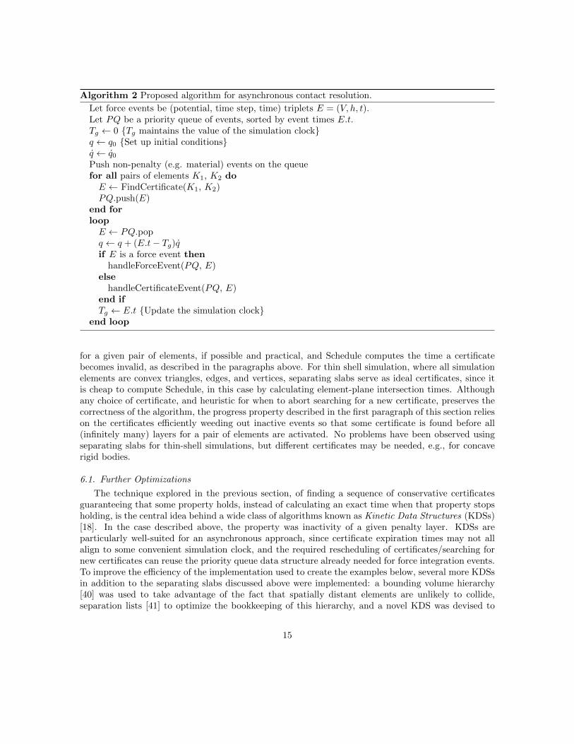
Algorithm 2 Proposed algorithm for asynchronous contact resolution.

Let force events be (potential, time step, time) triplets E = (V, h, t).Let PQ be a priority queue of events, sorted by event times E.t.Tg ← 0 {Tg maintains the value of the simulation clock}q ← q0 {Set up initial conditions}q ← q0Push non-penalty (e.g. material) events on the queuefor all pairs of elements K1, K2 doE ← FindCertificate(K1, K2)PQ.push(E)

end forloopE ← PQ.popq ← q + (E.t− Tg)qif E is a force event then

handleForceEvent(PQ, E)else

handleCertificateEvent(PQ, E)end ifTg ← E.t {Update the simulation clock}

end loop

for a given pair of elements, if possible and practical, and Schedule computes the time a certificatebecomes invalid, as described in the paragraphs above. For thin shell simulation, where all simulationelements are convex triangles, edges, and vertices, separating slabs serve as ideal certificates, since itis cheap to compute Schedule, in this case by calculating element-plane intersection times. Althoughany choice of certificate, and heuristic for when to abort searching for a new certificate, preserves thecorrectness of the algorithm, the progress property described in the first paragraph of this section relieson the certificates efficiently weeding out inactive events so that some certificate is found before all(infinitely many) layers for a pair of elements are activated. No problems have been observed usingseparating slabs for thin-shell simulations, but different certificates may be needed, e.g., for concaverigid bodies.

6.1. Further Optimizations

The technique explored in the previous section, of finding a sequence of conservative certificatesguaranteeing that some property holds, instead of calculating an exact time when that property stopsholding, is the central idea behind a wide class of algorithms known as Kinetic Data Structures (KDSs)[18]. In the case described above, the property was inactivity of a given penalty layer. KDSs areparticularly well-suited for an asynchronous approach, since certificate expiration times may not allalign to some convenient simulation clock, and the required rescheduling of certificates/searching fornew certificates can reuse the priority queue data structure already needed for force integration events.To improve the efficiency of the implementation used to create the examples below, several more KDSsin addition to the separating slabs discussed above were implemented: a bounding volume hierarchy[40] was used to take advantage of the fact that spatially distant elements are unlikely to collide,separation lists [41] to optimize the bookkeeping of this hierarchy, and a novel KDS was devised to

15

Algorithm 3 handleForceEvent

Require: Priority queue of events PQ and force event E that needs processing{Processing a force event E is a three-step process: integrating the force, rescheduling all eventswhose support depends on E’s stencil, and lastly, resceduling E itself.}for all i in Stencil(E) doqi ← qi − (E.h)M−1i

∂E.V∂qi

{Update only those elements affected by this event.}end for{Reschedule all events whose support depends on E’s stencil}for all Certificate events E′ with Stencil(E) ∩ Support(E′) 6= ∅ doPQ.remove(E′)Schedule(E′)PQ.push(E′)

end for{If E was a penalty force event, it exerted 0 force, and the two primitives in question are separating,then we no longer need it}if E is a penalty force event and ∂E.V

∂qi= 0 then

if E.V.K1 and E.V.K2 have positive relative velocity (are separating) thenreturn

end ifif addCertificate(E.V.K1, E.V.K2) then

returnend if

end if{Otherwise, reschedule E itself}PQ.push(V, h, t+ h)

Algorithm 4 handleCertificateEvent

Require: Priority queue of events PQ and certificate event E that needs reschedulingif not addCertificate(E.K1, E.K2) then{Finding a new certificate failed. We must thus activate a penalty force, one layer deeper thanthe deepest currently active penalty force event.}CurLayer ← max{penalty events E′ on queue for E.K1 and E.K2}E

′.layerE′ ← new PenaltyForceEvent(E.K1, E.K2, CurLayer + 1)PQ.push(E′) {Push the appropriate penalty force event on the queue}

end if

16

Algorithm 5 addCertificate

Require: Priority queue of events PQ, and two elements K1 and K2{Attempts to find a certificate for the collision of K1 against K2 and add it to the queue. Returnstrue if one was found.}E′ ← FindCertificate(K1, K2)if E′ was successfully found thenPQ.push(FindCertificate(K1, K2))return true

end ifreturn false

leverage the observation that high-frequency, low amplitude oscillations in velocity do not significantlychange a separation slab’s expiration time, so that rescheduling is in many cases unnecessary. All ofthe improvements are described in greater detail in [17].

7. Dissipation

The framework, as described so far, gives near-perfect long-time energy conservation. In the realworld, however, many dissipative phenomena are observed — for instance friction, spring damping,and non-unit coefficients of restitution during collisions. Several simple modifications can be madeto the proposed method to take such dissipation into account. Qualitatively, these have performedwell in practice: energy seems to behave well over long times for dissipative systems analogously tothe near-conservation observed for Hamiltonian systems, but a theoretical understanding of this goodbehavior remains future work.

7.1. Coefficient of Restitution

It is often desirable to simulate semi-elastic or inelastic collisions. A simple modification to thepotential Vl allows the use of arbitrary coefficients of restitution e:

Vl(q) =

{0 gη/l(q) > 0

l3ksgη/l(q)2 gη/l(q) ≤ 0,

where s is e if the primitives are separating, 1 otherwise. The penalty layers exert their full forceduring compression, then weaken according to the coefficient of restitution during decompression.

This approach, while simple, does have a limitation in the inelastic limit e = 0: due to errorintroduced by numerical integration, two colliding primitives may have non-zero, though small, post-response normal relative velocity. The magnitude of this velocity is at most kη/l, so it can be limitedby choosing a small enough base stiffness k.

7.2. Friction

The Coulomb friction model is a simple approximation to kinetic friction: at a point of contactbetween two bodies, the Coulomb force has magnitude µ|Fn|, where µ is a coefficient of friction andFn is the normal force at the contact points, and has direction opposite the relative tangential motionof the contact points.

17

0 2´107 4´107 6´107 8´107 1´108-0.5

-0.4

-0.3

-0.2

-0.1

0.0

0.1

0.2

Time H s L

Rel

ativ

eE

nerg

yD

evia

tion

Figure 2: The relative error in energy of a spring bouncing on a plane when a) the system is integrated by mixingvariational material force integration with impulse-based collision response (blue), b) the alignment of the integrationclocks is not respected (maroon), c) using the proposed method (brown).

Whenever an impulse is applied during integration of a penalty layer, a corresponding frictional im-pulse can also be applied. Just as increasingly stiff penalty forces are applied for contact forces, frictionforces are increasingly applied (equal to µ|Fn|) to correctly halt high-speed tangential motion. Noticethat these friction forces, like the material and contact penalty forces, are applied asynchronously:every layer applies friction independently at its own time step.

This simple, asynchronous formulation of friction fits very naturally into the framework of AVIs.Unfortunately, it is unsuitable for simulations featuring static friction, such as a block of wood restingon an inclined plane. The above formulation, with friction applied piecemeal during penalty inte-gration, is reactive instead of proactive, and in simulations of this type the block of wood has beenobserved “creeping” down the incline no matter how high a coefficient of restitution is chosen. A morecomprehensive model of friction compatible with the AVI framework, which correctly handles staticfriction, remains future work.

8. Results

8.1. Spring on a plane

As a simplest didactic demonstration of the proposed method, three experiments were conducted.A vertical spring of unit rest length, stiffness, and endpoint masses began each of the three simulationsstationary a unit height above a fixed horizontal plane. The springs fell under a gravitational force ofstrength 1m/s2, with impact handled in one of three different ways:

In the first experiment, gravity and the stretching force were integrated synchronously, and aninstantaneous impulse was applied whenever the bottom of the spring touched the plane. Figure 2shows error in energy over time when using this method. Energy in this experiment, far from beingconserved, took a random walk.

In the second experiment, all forces were integrated asynchronously using the proposed method.The thickness η was chosen to be 0.1, and the penalty base stiffness k, 1000. Energy in this case waswell-conserved over long time: although energy experiences high-frequency, low-amplitude oscillations,there was no drift.

The importance of respecting the integrity of each potential’s integration clock is highlighted inthe third experiment. Instead of adding a force event onto the priority queue at an integer multiple of

18

its time step, the events are added at the precise moment when each layer becomes active. As can beseen from the resulting plot of energy error (Figure 2), energy is no longer well-conserved, but insteadseems to increase monotonically over time.

8.2. Box of particles

Figure 3: A rigid box containing 900 spheres with random initial velocity, several minutes after the start of the simulation.

0 10 20 30 40 50

-0.0004

-0.0002

0.0000

0.0002

0.0004

Time H s L

Rel

ativ

eE

nerg

yD

evia

tion

0 10 20 30 40 50-0.02

-0.01

0.00

0.01

0.02

Time H s L

Rel

ativ

eE

nerg

yD

evia

tion

Figure 4: Left: The relative error in measured energy (brown) and momentum (orange), as compared to the samequantities at the start of the simulation, for the box of spheres. Right: The relative error of energy of the box, withgravity added, over time.

As an example that involves more collisions, consider a fixed 3 m× 3 m square box. Inside this box900 spheres of radius 10 cm were uniformly distributed, each of which was given a random velocity ofmagnitude between 0 and 10 m/s. Figure 3 depicts this box after several minutes have elapsed. Energyerror over time is plotted in Figure 4 (left), and it is again almost perfectly conserved. The same plotalso shows the error in total momentum of the box over time, and it is exactly zero, as expected sincea multisymplectic integrator is used. Gravity (9.8 m/s2) was added to the box and again the relativeerror of energy was plotted over time (Figure 4, right), Good behavior of the energy error was stillobserved.

19

0 5 10 15 200

50

100

150

Time H s L

En

erg

yH

JL

Figure 5: The energy of the box of 900 spheres under different coefficients of restitution: from top to bottom, 1.0, 0.9,0.8, 0.7, 0.5, 0.2, 0.0.

As a test of controllable dissipation by using a coefficient of restitution, the box with gravity wasresimulated several times using different coefficients of restitution. Figure 5 shows the resulting energyplots. For any chosen coefficient of restitution, the non-conservative energy behavior is qualitativelyas one would expect.

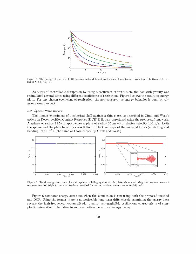
8.3. Sphere-Plate Impact

The impact experiment of a spherical shell against a thin plate, as described in Cirak and West’sarticle on Decomposition Contact Response (DCR) [34], was reproduced using the proposed framework.A sphere of radius 12.5 cm approaches a plate of radius 35 cm with relative velocity 100 m/s. Boththe sphere and the plate have thickness 0.35 cm. The time steps of the material forces (stretching andbending) are 10−7 s (the same as those chosen by Cirak and West.)

0

0.1

300.0100.00 0.004 0.005Time (s)

En

erg

y (

J)

0.2

0.15

0.05

0.0020

0.1

.00300.0010 0.004 0.005Time (s)

Ener

gy (J

)

0.2

0.15

0.05

0.002

0.001 0.0020.186300

0.186320

Figure 6: Total energy over time of a thin sphere colliding against a thin plate, simulated using the proposed contactresponse method (right) compared to data provided for decomposition contact response [34] (left).

Figure 6 compares energy over time when this simulation is run using both the proposed methodand DCR. Using the former there is no noticeable long-term drift; closely examining the energy datareveals the high-frequency, low-amplitude, qualitatively-negligible oscillations characteristic of sym-plectic integration. The latter introduces noticeable artifical energy decay.

20

8.4. Large-scale Three-dimensional Examples

Harmon et al. [17] describe a series of optimizations that improve the efficiency of Algorithm 2.These optimizations were incorporated to form our Asynchronous Contact Mechanics (ACM) code.This code continues to yield qualitatively good results when scaled to additional large-scale problems.

Figure 7: Simulated tying of a cloth reef knot (left) and bowline knot (right).

Two thin rectangular 27 cm× 2 cm ribbons were modeled as thin shells of 5321 vertices, subject toconstant-strain triangle stretching forces [42] (stiffness 750) and discrete shell bending forces formulatedby Grinspun et al. [43] (stiffness 0.05). These ribbons were positioned into a loose reef knot by anartist. The knot was then tightened by constraining the end of the ribbon to move apart at 10 cm/s,and running the simulation.

Figure 7, left, shows the ribbon after 2 seconds. Since the velocities of the ends of the ribbons wereconstrained, the knot material became arbitrarily stretched once the knot was tight. The forces pressingthe two ribbons into each other thus grew unbounded, but the two ribbons never interpenetrated, norwere other collision-related artifacts observed. It should be stressed that this good behavior did notrequire the tweaking of the penalty stiffnesses nor any other artificial parameters.

As a second large-scale example, a ribbon similar to the ones in the reef knot simulation waspositioned by an artist into a loose bowline knot tied around a cylindrical thin shell of 1334 vertices.The bowline was then tightened by fixing one end of the ribbon and constraining the other to moveaway from the cylinder at 10 cm/s. Again, the knot successfully tightened with no penetrations orother artifacts (Figure 7, right).

8.5. Sphere and Wedge

Inspired by Pandolfi et al. [10], a rigid thin-shell sphere was dropped into a wedged formed by twothin shell triangular prism, shown in Figure 8. Each prism has an isosceles base with width 12.92 cmand height 20.05 cm, and length 38.41 cm. The prisms contain 71 vertices each. The sphere contains92 vertices, has radius 4.97 cm and begins the simulation 20.84 cm above the ground plane on whichthe prisms rest. The sphere has initial downwards velocity of −100 cm/s (no gravity). The sphere andshells use the same thin shell model as the debris in the above trash compactor example, with bendingand stretching stiffness parameters 100000 and 50000 respectively.

As the sphere descends, it enters into multiple contact with the faces of the wedge, which undergoelastic deformation and high-frequency vibration. Despite the large areas of simultaneous contact and

21

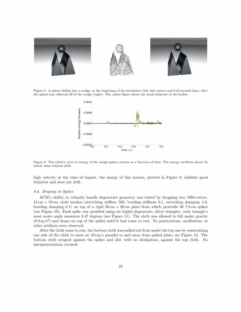
Figure 8: A sphere falling into a wedge, at the beginning of the simulation (left and center) and 0.42 seconds later, afterthe sphere has reflected off of the wedge (right). The center figure shows the mesh elements of the bodies.

0.0 0.1 0.2 0.3 0.4 0.5-0.0010

-0.0005

0.0000

0.0005

0.0010

Time H s L

Rel

ativ

eE

nerg

yD

evia

tion

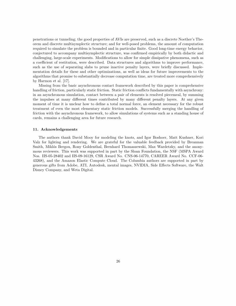
Figure 9: The relative error in energy of the wedge-sphere system as a function of time. The energy oscillates about itsinitial value without drift.

high velocity at the time of impact, the energy of this system, plotted in Figure 9, exhibits goodbehavior and does not drift.

8.6. Draping on Spikes

ACM’s ability to robustly handle degenerate geometry was tested by dropping two 1994-vertex,15 cm × 50 cm cloth meshes (stretching stiffnes 500, bending stiffness 0.1, stretching damping 1.0,bending damping 0.1) on top of a rigid 20 cm × 20 cm plate from which protrude 36 7.8 cm spikes(see Figure 10). Each spike was modeled using six highly-degenerate, sliver triangles: each triangle’smost acute angle measures 3.47 degrees (see Figure 11). The cloth was allowed to fall under gravity(9.8 m/s2) and drape on top of the spikes until it had come to rest. No penetrations, oscillations, orother artifacts were observed.

After the cloth came to rest, the bottom cloth was pulled out from under the top one by constrainingone side of the cloth to move at 10 cm/s parallel to and away from spiked plate; see Figure 12. Thebottom cloth scraped against the spikes and slid, with no dissipation, against the top cloth. Nointerpenetrations occured.

22

Figure 10: Two cloth rectangles were draped on a bed of spikes. The system at the start of the simulation (left), andafter the cloth has come to rest (right).

Figure 11: A close-up of one of the spikes; the spike has been rotated clockwise 90 degrees to conserve space. Each spikeis composed of six triangles with apex angle 3.47 degrees.

Figure 12: After the cloth came to rest, the bottom cloth was pulled out from under the top one. The simulation 3seconds after pulling began.

8.7. Trash Compactor

Various coarse thin-shell solid objects (platonic solids, tori, etc.) modeled as triangle meshes wereplaced in a rectangular box measuring 71.5 cm×36.7 cm×9.3 cm. The four sides were scripted to close

23

Figure 13: Walls close in and compress various thin-shell objects. The beginning (left) and end (right) of the simulation.

in and compress the objects within: the length at 20 cm/s, and the width at 10 cm/s. All objects weregiven the same material parameters (stretching stiffness 1000, bending stiffness 10, stretching damping15, bending damping 0.5) and held to the floor of the box by gravity (9.8 m/s2). Figure 13 shows thebox at the beginning of the simulation, and after the simulation had run for 3.4 seconds. A simpleplastic deformation model, described by Bergou et al. [44], allowed the objects to crush plasticallywhen stressed by the encroaching walls. Nevertheless, the material forces acting on the objects grewlarger as the box decreases to a small fraction of its original volume, yet no object penetrated anyother object or wall, as guaranteed by the method.

9. Effects of Stiffness and Thickness Parameters

The proposed algorithm requires choosing values for two parameters: k, the stiffness of the outer-most layer, and η, the outermost layer’s thickness. In penalty methods the choice of stiffness is oftencritical – there is no guaranteed maximum degree of constraint violation, so failure to judiciously setthe stiffness to a problem-dependent optimal value can result in arbitrary large penetrations and errorsin trajectories and, in the worst case, the tunnelling of objects through each other.

The proposed method using discrete penalty layers, by contrast, is guaranteed by constructionto prevent interpenetrations for any choice of stiffness parameter. Different choices of parametervalue do, however, affect the trajectory of the simulation – increasing the stiffness decreases the timeobjects are in contact during impact events, and more closely approximates exact enforcement of theconstraint gη > 0. Changing the stiffness also requires changing the time step of penalty force events toretain stability and good energy behavior. A full theoretical understanding of the relationship betweenstiffnesses and stable time steps for AVIs remains future work; for instance recent research [45] suggeststhat poorly chosen time step ratios can lead to resonance instabilities. Nevertheless, in practice,

24

a penalty time step proportional to 1√k

was observed to be stable for all experiments described in

Section 8.The choice of thickness η likewise does not affect the method’s non-interpenetration guarantee, but

does influence the trajectory, since shrinking η shrinks the distance over which the penalty layers arepermitted to act, approaching exact enforcement of the constraint g0 > 0 as the thickness vanishes.Moreover, since the maximum potential energy Vl of a layer l is proportional to η2, for smaller η stiffer,deeper layers will be activated to resolve a given collision, carrying a performance cost.

-4 -2 0 2 4-4

-2

0

2

4

X H m L

YHm

L

0 20 40 60 80 100-0.010

-0.005

0.000

0.005

0.010

Time H s LR

elat

ive

Ene

rgy

Dev

iatio

n

-4 -2 0 2 4-4

-2

0

2

4

X H m L

YHm

L

0 20 40 60 80 100-0.010

-0.005

0.000

0.005

0.010

Time H s L

Rel

ativ

eE

nerg

yD

evia

tion

Figure 14: The trajectory (left) and energy behavior over time (right) of a single ball bouncing elastically between twoparallel walls in two dimensions, for two different outer layer thicknesses (top row: η = 1 m; bottom row: η = 0.1 m)and three outer layer stiffnesses (solid line: k = 1; dashed line: k = 0.1; dotted line: k = 0.01). Although the choice ofthese parameters affects the trajectory of the system, good energy behavior is guaranteed for any such choice.

To explore the effects of k and η on a simple simulation, a particle in 2D of unit mass was simulatedbouncing between two parallel walls 1 m apart (no gravity). The particle was initially positionedmidway between the walls, with velocity 1 m/s at 85 degrees to the bottom wall. Figure 14 shows thetrajectory and energy of the particle for various choices of k and η.

10. Conclusion and Future Work

A framework for asynchronous, structure-preserving handling of contact and impact has been pre-sented. Provable guarantees were established for this framework: impact handling is robust, allowing no

25

penetrations or tunneling; the good properties of AVIs are preserved, such as a discrete Noether’s The-orem and discrete multisymplectic structure; and for well-posed problems, the amount of computationrequired to simulate the problem is bounded and in particular finite. Good long-time energy behavior,conjectured to accompany multisymplectic structure, was confirmed empirically by both didactic andchallenging, large-scale experiments. Modifications to allow for simple dissipative phenomena, such asa coefficient of restitution, were described. Data structures and algorithms to improve performance,such as the use of separating slabs to prune inactive penalty layers, were briefly discussed. Imple-mentation details for these and other optimizations, as well as ideas for future improvements to thealgorithms that promise to substantially decrease computation time, are treated more comprehensivelyby Harmon et al. [17].

Missing from the basic asynchronous contact framework described by this paper is comprehensivehandling of friction, particularly static friction. Static friction conflicts fundamentally with asynchrony:in an asynchronous simulation, contact between a pair of elements is resolved piecemeal, by summingthe impulses at many different times contributed by many different penalty layers. At any givenmoment of time it is unclear how to define a total normal force, an element necessary for the robusttreatment of even the most elementary static friction models. Successfully merging the handling offriction with the asynchronous framework, to allow simulations of systems such as a standing house ofcards, remains a challenging area for future research.

11. Acknowledgements

The authors thank David Mooy for modeling the knots, and Igor Boshoer, Matt Kushner, KoriValz for lighting and rendering. We are grateful for the valuable feedback provided by BreannanSmith, Miklos Bergou, Rony Goldenthal, Bernhard Thomaszewski, Max Wardetzky, and the anony-mous reviewers. This work was supported in part by the Sloan Foundation, the NSF (MSPA AwardNos. IIS-05-28402 and IIS-09-16129, CSR Award No. CNS-06-14770, CAREER Award No. CCF-06-43268), and the Amazon Elastic Compute Cloud. The Columbia authors are supported in part bygenerous gifts from Adobe, ATI, Autodesk, mental images, NVIDIA, Side Effects Software, the WaltDisney Company, and Weta Digital.

26

References

[1] A. Lew, J. Marsden, M. Ortiz, M. West, Asynchronous variational integrators, Archive forRational Mechanics and Analysis 167 (2003) 85–146.

[2] Y. Suris, Hamiltonian methods of runge-kutta type and their variational interpretation, Matem-aticheskoe Modelirovanie 2 (1990) 78–87.

[3] R. MacKay, Some aspects of the dynamics of hamiltonian systems, in: The Dynamics of Numericsand the Numerics of Dynamics, Oxford University Press, 1992, pp. 137–193.

[4] J. Marsden, M. West, Discrete mechanics and variational integrators, Acta Numerica 10 (2001)357–514.

[5] M. West, Variational integrators, Ph.D. thesis, California Institute of Technology, 2004.

[6] E. Hairer, C. Lubich, G. Wanner, Geometric Numerical Integration: Structure-Preserving Algo-rithms for Ordinary Differential Equations, Springer-Verlag, second edition, 2006.

[7] E. Barth, B. Leimkuhler, S. Reich, A time-reversible variable-stepsize integrator for constraineddynamics, SIAM Journal on Scientific Computing 21 (1999) 1027–1044.

[8] C. Kane, J. E. Marsden, M. Ortiz, M. West, Variational integrators and the newmark algorithmfor conservative and dissipative mechanical systems, International Journal for Numerical Methodsin Engineering 49 (2000) 1295–1325.

[9] T. A. Laursen, G. R. Love, Improved implicit integrators for transient impact problems - geometricadmissibility within the conserving framework, International Journal for Numerical Methods inEngineering 53 (2002) 245–274.

[10] A. Pandolfi, C. Kane, J. E. Marsden, M. Ortiz, Time-discretized variational formulations of non-smooth frictional contact, International Journal for Numerical Methods in Engineering 53 (2002)1801–1829.

[11] R. Rangarajan, R. Ryckman, A. Lew, Towards long-time simulation of soft tissue simulantpenetration, in: Proceedings of the 26th Army Science Conference, pp. 1–8.

[12] R. Ryckman, A. Lew, An explicit asynchronous contact algorithm (in preparation).

[13] P. Wriggers, Computational Contact Mechanics, John Wiley and Sons Ltd, 2002.

[14] T. Laursen, Computational Contact and Impact Mechanics, 2002.

[15] T. Belytschko, M. O. Neal, Contact-impact by the pinball algorithm with penalty and lagrangianmethods, International Journal for Numerical Methods in Engineering 31 (1991) 547–572.

[16] J. Nocedal, S. Wright, Numerical Optimization, Springer, 2000.

[17] D. Harmon, E. Vouga, B. Smith, R. Tamstorf, E. Grinspun, Asynchronous contact mechanics,in: ACM SIGGRAPH 2009 papers, pp. 1–12.

27

[18] L. J. Guibas, Kinetic data structures: a state of the art report, in: Proceedings of the ThirdWorkshop on the Algorithmic Foundations of Robotics on Robotics : the Algorithmic Perspective,pp. 191–209.

[19] H. Hertz, Study on the contact of elastic bodies, Journal fur die Reine und AngewandtheMathematik 29 (1882) 156–171.

[20] T. Belytschko, W. K. Liu, B. Moran, Nonlinear Finite Elements for Continua and Structures,John Wiley and Sons, 2006.

[21] P. Wriggers, Finite element algorithms for contact problems, Archives of Computational Methodsin Engineering 2 (1995) 1–49.

[22] J. T. Oden, Exterior penalty methods for contact problems in elasticity, in: Bathe, Stein, Wun-derlich (Eds.), Europe-US Workshop: Nonlinear Finite Element Analysis in Structural Mechanics,Springer, 1980.

[23] N. Kikuchi, J. T. Oden, Contact Problems in Elasticity: A Study of Variational Inequalities andFinite element Methods, SIAM, 1988.

[24] W. J. T. D. T. Belytschko, G. Ventura, A monolithic smoothing-gap algorithm for contact-impact based on the signed distance function, International Journal for Numerical Methods inEngineering 55 (2002) 101–125.

[25] D. Peric, D. R. J. Owen, Computational model for 3-D contact problems with friction basedon the penalty method, International Journal for Numerical Methods in Engineering 35 (1992)1289–1309.

[26] T. Hughes, R. L. Taylor, J. L. Sackman, A. Curnier, W. Kanoknukulchai, A finite element methodfor a class of contact-impact problems, Computer Methods in Applied Mechanics and Engineering8 (1976) 249–276.

[27] B. Nour-Omid, P. Wriggers, A two-level iteration method for solution of contact problems, Com-puter Methods in Applied Mechanics and Engineering 54 (1986) 131–144.

[28] R. L. Taylor, P. Papadopoulos, On a finite element method for dynamic contact/impact problems,International Journal for Numerical Methods in Engineering 36 (1993) 2123–2140.

[29] D. P. Bertsekas, Contrained Optimization and Lagrange Multiplier Methods, Academic Press,1984.

[30] P. Wriggers, J. C. Simo, R. L. Taylor, Penalty and augmented lagrangian formulations for con-tact problems, in: J. Middleton, G. N. Pande (Eds.), Proceedings of NUMETA 85 Conference,Balkema, 1985.

[31] J. C. Simo, T. A. Laursen, An augmented lagrangian treatment of contact problems involvingfriction, Computers and Structures 42 (1992) 97–116.

[32] J. C. Simo, P. Wriggers, R. L. Taylor, A perturbed lagrangian formulation for the finite elementsolution of contact problems, Computer Methods in Applied Mechanics and Engineering 50 (1985)163–180.

28

[33] C. Kane, E. A. Repetto, M. Ortiz, J. E. Marsden, Finite element analysis of nonsmooth contact,Computer Methods in Applied Mechanics and Engineering 180 (1999) 1–26.

[34] F. Cirak, M. West, Decomposition contact response (DCR) for explicit finite element dynamics,International Journal for Numerical Methods in Engineering 64 (2005) 1078–1110.

[35] C. Lanczos, The Variational Principles of Mechanics, Dover Publications, fourth edition, 1986.

[36] A. Lew, Variational Time Integrators in Computational Solid Mechanics, Ph.D. thesis, CaliforniaInstitute of Technology, 2003.

[37] A. P. Veselov, Integrable discrete-time systems and difference operators, Functional Analysis andIts Applications 22 (1988) 83–93.

[38] J. Moser, A. P. Veselov, Discrete versions of some classical integrable systems and factorizationof matrix polynomials, Communications in Mathematical Physics 139 (1991) 217–243.

[39] J. M. Wendlandt, J. E. Marsden, Mechanical integrators derived from a discrete variationalprinciple, Physica D: Nonlinear Phenomena 106 (1997) 223–246.

[40] J. T. Klosowski, M. Held, J. S. B. Mitchell, H. Sowizral, K. Zikan, Efficient collision detectionusing bounding volume hierarchies of k-dops, IEEE Transactions on Visualization and ComputerGraphics 4 (1998) 21–36.

[41] R. Weller, G. Zachmann, Kinetic separation lists for continuous collision detection of deformableobjects, in: Third Workshop in Virtual Reality Interactions and Physical Simulation (Vriphys).

[42] Y. Gingold, A. Secord, J. Y. Han, E. Grinspun, D. Zorin, A Discrete Model for Inelastic Defor-mation of Thin Shells, Technical Report, New York University, 2004.

[43] E. Grinspun, A. Hirani, M. Desbrun, P. Schrder, Discrete shells, in: Proceedings of the 2003ACM SIGGRAPH/Eurographics symposium on Computer animation, pp. 62–67.

[44] M. Bergou, S. Mathur, M. Wardetzky, E. Grinspun, Tracks: toward directable thin shells, in:ACM SIGGRAPH 2007 papers, p. 50.

[45] W. Fong, E. Darve, A. Lew, Stability of asynchronous variational integrators, in: Proceedings ofthe 21st International Workshop on Principles of Advanced and Distributed Simulation, PADS’07, pp. 38–44.

29