PART I

ON THE BREAKING OF NONLINEAR DISPERSIVE WAVES

PART II

VARIATIONAL PRINCIPLES IN CONTINUUM MECHANICS

Thesis by

Robert L. Seliger

In Partial Fulfillment of the Requirements

For the Degree of

Doctor of Philosophy

California Institute of Technology

Pasadena, California

1968

(Submitted November 10, 1967)

-n-

ACKNOWLEDGEMENTS

The author wishes to thank Professor G. B. Whitham for

suggesting these topics and for providing guidance, many useful

suggestions and invaluable criticism during the course of this

research.

The financial support of the author's graduate education was

attained through the Fellowship Programs of the Hughes Aircraft

Company. The author is sincerely grateful for having participated

in these programs and would like to thank all the people who made

this possible. The author especially thanks the Fellowship

representative with whom he had most contact , Mrs. D. M cClure

of the Hughes Research Laboratories, for consistently providing

accurate, efficient and outstandingly pleasant administration of the

Programs. Special thanks also go to Mr. J. H . Molitor of the Hughes

Research Laboratories for complementing the author's academic

education with insight into the real world and for being so generously

re ce ptive to the toils and troubles of students.

Finally, the author acknowledges an extremely competent

and cheerful typist, Miss Ann Law of the Hughes Research

Laboratories for typing this dissertation.

-111-

ABSTRACT

A model equation for water waves has been suggested by

Whitham to study , qualitatively at least, the different kinds of

breaking. This is an integra-differential equation which combines

a typical nonlinear convection term with an integral for the

dispersive effects and is of independent mathematical interest.

For an approximate kernel of the form -blxl e ' it is shown

first that solitary waves have a maximum height with sharp

crests and secondly that waves which are sufficiently asymmetric

break into "bores. 11 The second part applies to a wide class of

bounded kernels , but the kernel giving the correct dispersion

effects of water waves has a square root singularity and the

present argument does not go through. Nevertheless the

possibility of the two kinds of breaking in such integra-differential

equations is demonstrated.

Difficulties arise in finding variational principles for

continuum mechanics problems in the Eulerian (field) description.

The reason is found to be that continuum equations in the original

field variables lack a mathematical ''self-adjointness 11 property

which is necessary for Euler equations. This is a feature of

the Eulerian description and occurs in non-dissipative problems

which have variational principles for their Lagrangian description.

To overcome this difficulty a ''potential representation'' approach

is used which consists of transforming to new (Eulerian) variables

whose equations are self-adjoint. The transformations to the

-lV-

velocity potential or stream function in fluids or the scaler and

vector potentials in electromagnetism often lead to variational

principles in this way. As yet no general procedure is available

for finding suitable transformations. Existing variational

principles for the inviscid fluid equations in the Eulerian

description are reviewed and some ideas on the form of the

appropriate transformations and Lagrangians for fluid problems

are obtained. These ideas are developed in a series of examples

which include finding variational principles for Rossby waves

and for the internal waves of a stratified fluid.

-v-

TABLE OF CONTENTS

PART PAGE

I. ON THE BREAKING OF NONLINEAR DISPERSIVE

WAVES

1. Introduction 1

2. Solutions with Sharp Crests 3

3 . Solutions which Break into Bores 7

II. VARIATIONAL PRINCIPLES IN CONTINUUM

MECHANICS

4. Introduction 12

5. The Self-Adjointness Condition of Vainberg 18

6. A Variational Formulation of In viscid

Fluid Mechanics . . 25

7. Variational Principles for Ross by Waves in

a Shallow Basin and in the "13-P.lane" Model . 37

8. The Variational Formulation of a

Plasma .

9. Variational Principles for the Internal Waves

of a Stratified F'luid .

APPENDIX A

APPENDIX B

The Singularity in K (x) g

An Estimate of p(x, t) for a

Breaking Wave

. 49

53

59

. 61

-1-

PART I

ON THE BREAKING OF NONLINEAR DISPERSIVE WAVES

1. Introduction

An integra-differential equation has been proposed by

Whitham [ 1] which offers an improvement on the well known

Korteweg-de Vries equation for water waves. This integral equation

can be considered an extension of the (relatively long wave)

Korteweg-de Vries model to include all the dispersion present in

linear water wave theory. The Korteweg-de Vries equation ( 2] is

"lt+(a"l+c )"1 +y"l = 0, 0 X XXX

where "1 1s the elevation of the water surface above the undisturbed

depth h, 0

a = 3c /2h , 0 0

1 2 c = ~, and 'I = -

6 c h .

0 0 0 0 This

equation is valid for water waves whose typical amplitude a and

2 2 wavelength X. are such that a/h and h /X. are comparable small

0 0

quantities. The form of the proposed extension is

<X)

"lt+a"l"lx+J K(x- £)"1~(£,t)d£ = 0.

-oo

( 1)

1. G. B. Whitham, Proc. Roy. Soc. A, Vol. 299 ( 1967) pp. 6-25.

2.. D. J. Korteweg and G. de Vries, Phil. Mag., Vol. 39 ( 1895), pp. 422-443.

-2-

For water waves the appropriate kernel is the Fourier transform

of the linear water wave phase speed c(k);

K(x) 1

= K (x) = g 2'TT

co

J -co

If only the first two terms

ikx c(k)e dk, c(k)

c 0

2 y k , in the long wave (kh << 1)

0

expansion of c(k) are used, equation ( l ) reduces to the

Korteweg-de Vries equation. It is known that two kinds of breaking

are observed for water waves: formation of sharp crests and

breaking into bores. Although the Korteweg-de Vries equation

has solitary wave and cnoidal wave train solutions, breaking of

solutions into sharp crests or bores has not been found. Apparent-

ly the 'llxxx term prevents these high frequency effects from

occurring. No theory has yet been given which demonstrates both

types of breaking. The more general equation ( l) was proposed

with the hope for finding these high frequency effec ts.

The water wave kernel K (x) has a square root singular­g

ity [ 3] which makes the integral in (l) difficult to handle. To

gain insight into the behavior of the solutions to such integral equa-

tions, the kernel will be approximated by functions of the form

-b\xl e .

3. See Appendix A.

-3-

2. Solutions with Sharp Crests

Uniformly propagating solutions of (1} are found with

'l = 'l(X), where X = x - Ut. For these solutions ( 1} can be

integrated once to the form

l 2 A - U'l + l o.'l +

(X)

J K(X- ~} 'l(~) d~ = 0,

-(X)

where A is the constant of integration. Oscillatory and solitary

wave solutions can be found for (2). But unlike the Korteweg-de

( 2}

Vries equation, (2) has maximum amplitude wave solutions which

have sharp crests. Solitary wave solutions can be distinguished

from oscillatory wave trains by requiring that 'l > 0 and 'l -0

as lxl - oo. Thus, to study solitary waves we take A= 0. Then,

by writing (2) in the form

(X)

( i a. 'l - U) 'l + f K( X - ~} 'l( ~} d~ = 0 ,

-(X)

it is seen that for a positive kernel, the height of solitary wave

solutions must be less than 2 u . 0.

(3}

More detailed investigations of (3) can be made for special

kernels. Whitham [ 4] discusses the occurrence of a sharp crest

in the maximum amplitude solitary wave solution to (2) for a kernel

of the form e -b lx I. This limiting solution can be found explicitly.

4. Ibid.

-4-

For the kernel e-bjxj (3) becomes a second order ordinary di£-

ferential equation when operated on by The

resulting equation can be integrated once and written in the form

1 b2,., 2 ( ) ( ) = 4 ., 11 - 111 11 - 112 • ( 4)

where the constant of integration is again zero (for solitary waves) .

If the precise kernel used to obtain {4) is

then 111

and 112

are the two roots of the quadratic equation

2 {a'll) + 4(a - U) a 11 + 2U(2U - 3a) = 0

and are given by the formulas

, 1 =

2

2a a.

Solitary wave solutions of {4) occur for real roots of the same

sign. It can be shown that a family of smooth solitary wave solu-

tions exists when the speed U lies in the range

3 2 a < U < 2a .

This corresponds to roots 111

, 112

which satisfy

-5-

o < "12 < ~ < "11 ·

These smooth solutions can be given implicitly in terms of

Jacobian elliptic functions and have maximum height equal to 112

.

3 The speed U = Z a gives 11

2 = 0 and the trivial solution. As

U - 2a both roots approach the value U/a.. When U = 2a the

maximum amplitude solitary wave occurs. Equation (4) reduces

to

,2 1 b2 2 "1 = 4 "1

which giy es a solution of the form -~lxl

e 2 It can be verified

directly that

u = 2a

is a solution of the integral equation (3) for the kernel K (x). ab

This solitary wave solution has a finite angle at the crest and

agrees qualitatively with observed water wave profiles [ 5].

To check the properties of this solution quantitatively

(5)

Whitham [ 6] chooses a = 2/3 and b - = rr/2 so that the kernel

Kab(x) models the water wave

proximation is poor near x =

kernel K (x). g

0 where K g

(Of course, the ap-

is singular.) The

value a.= 3/2 is taken to agree with the Korteweg-de Vries equation

5. See, for example, J . J. Stoke:+, Water Waves, sec. 10. 10. New York: Interscience (195 7).

6. Ibid.

and g = h 0

( 5) becomes

-6-

= l. Now the limiting solitary wave solution

which has a crest angle of 110° and a maximum height of 8/9.

Whitham points out that although these values agree reasonably well

with Stokes' 12.0° angle and McCowan's maximum height 0. 78,

the angle result should not be taken seriously since the angle size

depends on the local behavior of the kernel near x = 0. The

maximum height result depends on the whole kernel and may be

taken more seriously.

-7-

3. Solutions which Break into Bores

For approximate kernels progress can also be made on

proving that solutions of ( l) can break asymmetrically into bores.

The analysis is carried through for kernels which are bounded,

integrable, even functions of x which approach zero monotonically

as x approaches infinity. This includes a kernel such as

but does not include K (x) because of the singularity at x = 0. g

Sufficient conditions on the initial profile are found which guarantee

that the corresponding solution to ( l) breaks. The approach is

motivated from the hyperbolic equation

1lt + O.l)T)x + ~ 1') = 0, l3 > 0 • (6)

In this case, a method for seeing how solutions ca'n break is to

study the differential equation for the maximum value of -71 • Let X

m(t) denote this most negative slope and m(t) = 71 (X(t), t), where X

X(t) satisfies 71 (X( t), t) = XX

0. The ordinary differential equation

for m( t)

dm dt = - m(a.m + ~), (7)

is then obtained by differentiating (6) with respect to x and

setting x = X(t). The solution of (7) is

m(t)

-8-

where m = m( 0) is the most negative slope on the initial profile 0

,.,(x, 0). It is seen that if m < -~ breaking occurs (m(t) - co) 'I 0 Q. '

as t ..- ~log {<a.m0

)/(a.m0

+ 13)}. The significance of the breaking

condition m < -13/a. is that it ensures that the right hand side 0

of (7), and thus dm/dt, is negative initially. With m(O) and

dm(O)/dt negative, m(t) continues to decrease and the dominant

2 term -a.m gives m ..- - co in a finite time.

This same kind of dynamical breaking is found for the

nonlinear dispersive equation ( 1 ), but the initial conditions required

to start the steepening process are different and the argument has

to be extended. It is clear that important differences come in when

one takes into account that ( l), unlike ( 6 ), has nonbreaking

solutions with steady profiles. The oscillatory nature of these

solutions indicates that consideration of the maximum positive

slope will also be required. Let m _ ( t) be the most negative slope

of the solution T)(x, t) to ( l ). As before m ( t) = T) (X ( t), t), - X -

where X_ ( t) satisfies

satisfies the equation

where

co

p(x, t) = f -co

,., (X (t),t) = 0. ' 1xx -

dm

crt= 2

- a.m

K( £)TJ (x- £ , t)d£, XX

However, now m

p ( t)

p _( t) = p(X_(t), t) •

( 8)

-9-

Equation (8) governs breaking for the dispersive equation ( 1) as

(7) does for the hyperbolic equation (6). If steepening is to occur

in a similar way the -am: term must dominate p (t). Bounds on

p are therefore needed for this study and, since p(x, t) is linear

in T] the situation looks hopeful. Using the second mean value

theorem [ 7], p(x, t) can be written as

where s 1

and £2 are two numbers which depend on x and t and

satisfy sl :s x, Sz ~ x. A linear bound for p(x, t) in terms of

m_(t) and the maximum value of the positive slope m+(t) is then

I p( x, t) I :S K( 0) ( m + ( t) - m _ ( t)) ;

this inequality holds for all x. The essential difference between

(7) and (8) is the presence of m+(t) in the bound for p_. The

function m+(t) enters in such a way that it makes the right hand

side of (8) more positive and therefore deters breaking. An

estimate for m +( t) is found by considering its equation,

( 9)

( 1 0)

7. See, for example, E. W. Hobson, The Theory of Functions of a Real Variable, Vol. 1, p. 618. New York: Dover {1927).

-10-

where p+(t) = p(X+(t), t) and X+(t) satisfies "lxx(X+(t), t) = 0.

From the estimate in (9), the derivatives of m_(t) and m+(t)

can be bounded by

2. ~ - um + K( 0) { m + - m ) ,

dm+ 2. dt ~ -um+ + K(O) (m+- m_) .

Then

If m+ + m_ < - 2.K(O)/u initially, then m+ + m_ decreases

further and

< _ 2.K(O) for all t > 0. u

Using this estimate for m+ in (11), we have

dm

crt 2.

~ - um - 2.K(O)m

from which

( 11)

( 1 2.)

(13)

follows. Let q(t) = - (m_(t) + K~O)) and note that q > 0 when

2. ( 13) is satisfied. Therefore dq/ dt ~ uq and

where q = q > 0 at t = 0

-11-

l l :$ - a.t +-

q qo

o. Finally, for q we have

q ;:: l - uq t

0

l - ro as t-­

a.qo

We conclude that if the initial wave profile is sufficiently

asymmetrical so that m+(O) + m_(O) < - 2K(O)/a., the slope m_(t)

will become infinite in a time less than ja.m_(O) + K{O) r 1• This

is a sufficient condition only, not a sharp criterion.

For the kernel K {x) a proof that solutions of ( l) can g

break into bores is not yet available. One would like to carry

through similar arguments, but the extension of the proof is difficult;

the singularity in K {x) prevents the a priori estimate (9) of the g

integral p _ in terms of slopes. However, even with the infinity in

K (x) it seems likely that p is dominated by the term -am 2_ in

g -

{8) and can not prevent breaking of sufficiently asymmetric waves.

A partial indication of this is that if a typical breaking profile is

substituted into the integral it can be shown [ 8] that

p_ = o{jm_j7

/4

) as lm_l- ro.

8. See Appendix B.

-12-

PART II

VARIATIONAL PRINCIPLES IN CONTINUUM MECHANICS

4. Introduction

The variational formulation of classical mechanics provides

an elegant setting in which the deep ideas of dynamics, such as

canonical transformations and adiabatic invariants, can be concisely

expressed. Hopefully, a variational formulation of continuum

mechanics would be equally as fruitful. But the slow progress 1n

this direction indicates that new problems arise. When Hamilton 1s

principle is applied to the particles of a continuum, a variational

formulation does result which correctly gove rns motion of the

continuum as described by Lagrangian (or particle) coordinates.

But in many continuum problems, for example in fluid mechanics,

it is preferable to study the equations which correspond to Eulerian

(or field) coordinates. To obtain these equations .as they stand as

the Euler equations of some variational principle is generally

impossible. The reason is that in their original form the continuum

equations for field quantities generally do not satisfy a self-

adjointnes s condition. This condition is an extension of the usual

self-adjointness property to nonlinear operators and was

established as a necessary and sufficient condition for Euler

equations by Vainberg [ 9]. This is why existing variational

9. M. M. Vainberg, Variational Methods for the StudT of Nonlinear Operators. Transl. by A. Fe ins tein,Holden- Day 1964).

-13-

principles usually appear in terms of auxiliary quantities (e. g ., the

velocity potential and stream function in fluids or the vector and

scaler potentials in electromagne tism) whose equations are self­

adjoint .

Equations which are not self-adjoint can only come indirectly

from variational principles . Several different approaches to indirect

formulations are possible. A formulation in which the Lagrangian

for any equation of the form

Mu( x ) = 0 ( 14)

is immediately known, 1s to vary u in the functional

(15)

Sinc e J( u] takes on its minimum value zero for solutions of ( 14),

its Euler equation must be satisfied by solutions of ( 14). However,

th e actual Euler equation for J( u] 1s more complicated than

equation ( 14). For a linear operator L the functional J( u]

b e comes the inner product (Lu, Lu) whose Euler equation is

L>.'<Lu = 0, where L* istheoperatoradjointto L. Inthecase

of the heat equation,

the functional J( u) is

ff< uxx - ut) 2 dxdt

and the corresponding Euler equation is

-14-

c:~ -:,)(a:~ + :, ) u = 0 .

Thus, in this approach the functional to be varied is easily

formulated and the difficulty is that information about the original

equation is hidden in a more complicated Euler equation.

Another indirect variational technique is to vary only part

of the Lagrangian. To illustrate this approach we consider the

equation

"V • (A.( T) "V T) = 0 (16)

which arises in problems of steady-state heat conduction in a

solid. In such problems (16) is to be solved for the temperature

distribution T (x) in a body. The kind of variational principle o-

that we have in mind now is to find a functional ci>[ T , T], de­o

pending on the two functions J' 0

and T, for which the condition

( 17)

leads to equation (16). The meaning of (17) is that T is

varied in ci>( T , T) while T is treated as a known function. 0 0

Then, in the resulting Euler equation, T is set equal to T • One 0

functional which leads to ( 16) in this way is

( 18)

-15-

where A = A.(T }. Varying T in (18} gives 0 0

which becomes (16) with T = T. 0

Another functional which

also leads to (16} by this method is given by the integral

f A \7 T · ~ T dx . 0 0 -

The above example is taken from a paper by Glansdorff and

Prigogine [ 10] where a theory is presented which arrives at

the functional <r>(T , T) given in (18). Indeed some basis for 0

( 19)

choosing the most advantageous functional for a given equation would

be desirable. In this kind of variational technique the equations ob-

tained are precisely the ones of interest but the functionals used

depend on the solutions of the problems.

The approach to be considered here for finding indirect

variational principles is to introduce new dependent variables by

means of "potential" representations which result in self-adjoint

equations. Variational principles in terms of the potentials are

then found which have Euler equations equivalent to the original

non-self-adjoint set. The ideas of adiabatic invariants and

canonical transformations do occur in continuum problems for

which potential type variational formulations are used. In his

10. P. G1ansdorff and I. Prigogine, Physica, Vol. 30 ( 1964), pp. 351-374.

-16-

averaging method for nonlinear dispersive equations, Whitham [ ll]

finds that a prohibitive amount of algebra is avoided if the whole

theory is obtained from a variational formalism. The variational

principles he uses are of this potential repr esentation type and the

ideas of his theory then follow the lines of adiabatic invariants in

classical Lagrangian- Hamiltonian mechanics . Clebsch [ 12] gives

the first variational formulation of rotational fluid flow by

introducing a velocity representation of the form

Under this transformation the new equations of motion can be put

in a canonical form which resembles the classical Hamilton

equations [ 13]. The difficult steps in the potential representation

method are to find a suitable representation and to find a

Lagrangian which leads to the appropriate equations for the

potentials . A very general (one to one) representation is not always

required. For special problems such as irrotational flow , the

limited velocity potential representation u = \Tp is adequate and

the work in fi nding the variational formulation is reduced. There

11. G. B . Whitham, Proc. Roy. Soc. A, Vol. 283 ( 1965), pp . 238-261. J. Fluid Mech., Vol. 22 (1965), pp. 273 - 283.

12. A. Clebsch, J. reine u. angew. math., Vol. 56 (1859), pp. 1-10.

13. See , for example , H . Lamb, Hydrodynamics , 6 ed., p. 249, New York: Dover (19 32 ).

-17-

are, however, interesting examples for which more general

potential representations are required. This is true for Rossby

wave s and internal wave s which are examples of nonlinear

dispersive waves that can only exist in rotational fluid flows. The

model equations used to study these waves are approximate forms

of general equations for an inviscid fluid. Variational formulations

for these examples are found (Section 4, 6) by first studying the

variational formulation for a general inviscid fluid (Section 3) and

then suitably modifying the potential repre s entation and

Lagrang ian .

The discus sion begins {Section 2) with a brief account of

Vainber g 1 s necessary and sufficient self-adjointnes s condition for

Euler equations and its application to differential equa tions.

-18-

5. The Self-Adjointnes s Condition of Vainberg

Necessary and sufficient conditions for a class of nonlinear

equations to be the Euler equations of a variational principle have

been given by Vainberg [ 14]. Although Vainberg's work deals mostly

with nonlinear integral operators, his results are easily applied to

the partial differential equations of physics with which we are

concerned. This theory will now be discussed in terms of a single

ordinary differential equation of the form

F(u , u , u , x) = 0 , X XX

( 20)

where F 1s a polynomial function of the dependent variable u, its

first and second derivatives, and the independent variable x . Such

a limited model example can be used because extension of the ideas

to systems of nonlinear partial differential equations is straight-

forward. Vainberg found that the conditions for (20) to result from

the variation of some functional are analogous to the conditions for

a vector function to be the gradient of some scalar function. It is

well known that in three dimensions a vector can be expressed as

the gradient of a scalar if its curl is zero or, by Stoke's theorem,

if the line in te gral of the vector around any closed curve is zero.

To generalize the ''curl'' condition the notion of the derivative of an

operator is needed. Here it is useful to define

lim N (u + <Jh) - N(u) <J--0 (}

DN(u;h)

14. Loc. cit.

-19-

as the derivative of the operator N at the point u , in the direction h.

For operators such as F in ( 20 }, one recognizes that DF(u;h} 1s

just the operator F linearized about u operating on h . The

analogy to the "curl 11 condition is that for an operator F to come

from varying some functional, F must satisfy the symmetry

condition

(21)

at each point u and for all h1

and h2

. The inner products in (21}

are usual integrals over x . Condition ( 21) means that when F is

linearized about any point the resulting operator is self-adjoint. For

linear operators F = Lu, DF(u;h} = Lh, and (21} reduces to the

usua l definition of self-adjointness. Vainberg also defines the

concept of a curvelinear integral in function space for an operator

and shows that the independence of this integral on path determines

when the operator is an Euler equation. The definitions of these

function space concepts will not be needed here. We just note for

motivation that if the operator F has the path independence property,

its integral along any curve in function space, between the points 0

and u, say, must equal the straight line integral in function space

be tween 0 and u. But this straight line integral can be written

explicitly as

l 'I (F(A.u), u} dA. = J [ u] ,

0

( 2 2)

-20-

where again the inner product is an integral over x. Thus the

functional J[ uJ 1n (22) should be an excellent candidate for a

Lagrangian for F.

It will now be shown that (21) is indeed a necessary and

sufficient condition for (20} to come from a variational principle,

and that the Lagrangian is given in (22}. Suppose that F satisfies

the self-adjointnes s condition ( 21 }. Computing 6J[ uJ from ( 22}

gives

1 x2

OJ[ u] = I f k(>-u, kux' kuxx' x)Ou + kuDF(ku;Ou) ( dxdk

0 x1

By the sel£-adjointness of F it follows that

hence

x2 f ku DF(ku; Ou)dx

xl

x2

= J Mu DF(>-u, u)dx

xl

F(Au, AU , Au , x} 6u dx; X XX

. l x2

0 J[ u] = i J lF(ku, kux' kuxx' x) + >- ..& F (ku, kux' kuxx' x)i Oudxd>-

0 x 1 .

-21-

Assuming that the variations ou vanish at x1

and x2

, interchange

the order of integration and integrate the second term by parts with

respect to >... to obtain

oJ( u]

x2 .

= J F ( u, u , u , x) ou dx . X XX

xl

The variational principle 6J[ u) = 0 therefore leads to (20) as

its Euler equation. Conversely, suppose that F = 0 - is the Euler

equation from the variational principle

x2

of o((u,ux,x)dx = 0

xl

Then F must have the. form

F( u, u , u , x) = ;(. - ~;;(. ) • X XX U U

X X

The deriva tive of F 1s now given by

DF(u;h) = X h+X h UU UU X

X -( ;;:u h +X u hx) ~ X X X X

It is a straightforward calculation to show that

h1

DF(u;h) = h DF(u;h1

) ,

from which the self-adjointness of F follows.

(23)

-22-

When F is the expression in ( 23) J[ u] becomes

The second term can be integrated by parts to give

J( u] + u ;t X U

X

Since the second and third integrals do not contribute to the

variations, J[ u J is equivalent to the original Lagrangian.

To extend the above theory to systems of nonlinear partial

differential equations it is convenient to introduce vector notation.

Denote a system of partial differential equations by

( 24)

where

-23-

The F . are again polynomial functions of the dependent varia bles 1

u1

, u2

, .•• , un, their derivatives and the independent variables

• • • I X • n The derivative of the vector operator F

defined by

DF.(u:h) = 1--

lim <T-0

F.(u + <Th)- F .(u) 1- - 1-

0"

The self-adjointness condition for F is then

where the inner product is defined by

1s now

-24-

Using this definition of the inner product, the generalization of

the functional J [ u] in (22) is

1

J[ u] = J (F (X.~).~) dX.

0

With these definitions the results obtained for ( 20) are also

true for ( 24).

-25-

6. A Variational Formulation of Inviscid Fluid Mechanics

Variational principles for non-dissipative fluid flows de­

scribed in terms of Lagrangian (or particle) coordinates are known

to be the generalization of the classical Hamilton's principle for

a system of particles. The appropriate Lagrangian density has

the form of kinetic energy - internal energy for a fluid particle

and is a function of the position and velocity of the particle. In

these variational principles the particle paths themselves are

varied to give the necessarily self-adjoint Lagrangian equations

for the fluid. Variational principles for fluid flows described in

the more usual Eulerian (field) coordinates are more difficult.

The fluid equations in Eulerian coordinates are not self-adjoint as

they stand and therefore cannot be the Euler equations of a

variational principle in which the field quantities are varied. For

this reason the most common variational principles in fluid

mechanics appear for special flows in which new variables, such

as the velocity potential or stream function , can be introduced. The

advantage is that when the Eulerian equations are written in terms

of these auxiliary variables, they often become self-adjoint.

Although one usually looks at specialized flows, knowing a change

in variables which leads to variational principles for the general

fluid equations is useful when treating new problems.

Clebsch [ 15] introduced the representation

15. Loc. cit.

-26-

and was successful in finding a variational formulation for

incompressible rotational flow. He was motivated to introduce

the potentials p, a., ~ in the form of ( 25) from the results of

Pfaff's theorem [ 16] which states that the differential form

ud.x + vdy + wdz

1s reducible to a form

Equating the expressions m (26) and {27) leads to Clebsch's

representation ( 25 ). Clebsch finds that a variational formulation

of the equations

Du

Dt = - \7 p •

\7• u = 0 •

where

u = {u, v, w)

D a Dt = at + u· \7

'

16. See, for example, A. R. Forsyth, Theory of Differential Equations, Vol. l, New York: Dover {1959).

(25)

(26)

{27)

( 28)

-27-

is obtained by introducing the representation

(29)

( 3 0)

for the dependent variables. From ( 28) it follows that the

equations to be satisfied by ~. a, 13 are

Da 0 Dt =

.!2Q. = 0 Dt ( 31)

_'V · u= 0

where u stands for the expression in (29). Equations (31)

follow from varying ~. a, 13 in the variational principle

Here, as in all of the subsequent variational principles considered,

the Lagrangian is an integral over a fixed region of (~, t) spac e

and the variations are assumed to vanish on the boundary of this

region. This is the first instance in which the pressure appears

as the Lagrangian density. As will be seen in the later examples,

-28-

the pressure, expressed in terms of the potentials used, is the desired

Lagrangian density for problems in fluid mechanics described by

Eulerian coordinates, much the way the kinetic energy - potential

energy, expressedin terms of coordinates and velocities, is the

Lagrangian for problems in classical mechanics.

The potentials a., f3 account for circulation in the flow.

Expressions for the vorticity components in terms of a. and f3 are

s =

'l =

s =

w - v = y z

u - w = Z X

v - u = X y

8(a.,f3) 8(y,z)

8(a.,f3) 8( z, x)

8(a.,f3) a(x, y)

w = (£,1), s) = Y'a. X'Vf3 .

The intersection of surfaces a. = constant, f3 = constant

represents a vortex line . The first two equations in (31) indicate

that a. and f3 are constant following particles. Therefore vortex

lines move with the fluid and always carry the same particles. The

:role of the potentials a., f3 as ca,nonical variables is discussed by

Lamb [ i 7]. This propel'ty is also d:l.scussed by

17. Loc. cit.

-29-

Clebsch [ 18) with his ideas on canonical transformations of these

potentials. Here, it will only be remarked that if an arbitrary

function H(a., 13, t) 1s added to the pressure in (30) the equations

to be satisfied by the new potentials take on the canonical form

~ Dt = - H (a., ~. t) , a.

and follow from varying the integral of the new expression for the

pressure.

An extension of the above variational formulation to a

compressible fluid is given by Bateman [ 19]. His results are for

a so-called baratropic fluid in which the pressure is a function of

the density . The equations for compressible flow are

Du P nt = 'V p ,

~ + p 'V· u = 0 ,

18. Loc. cit.

( 3 2)

(33)

19. H. Bateman, Partial Differential Equations, p . 164, Cambridge: Cambridge University Press ( 1964).

-30-

and for convenience p(p) 1s taken to be of the form

I

p = p f ( p) - f( p) ( 34)

To obtain a variational formulation for (32) and (33), Bateman

uses the representation

u = 'Vp+ a'\713, ( 3 5)

(36)

Now the potentials p, a, 13 must satisfy the equations

Da 0 ' Dt =

~ Dt = 0 ' (37)

l2£. + p Dt '\7•u = 0 '

where u · stands for the expression in ( 35 ). Again, the variation

of p, a and l3 in the integral of the expression for the pressure

1n (36) leads to the set (37). The variation of p in this integral

leads to ( 34).

The first variational formulation of fluid mechanics in the

Eulerian description which includes all the effects of compressibility,

-31-

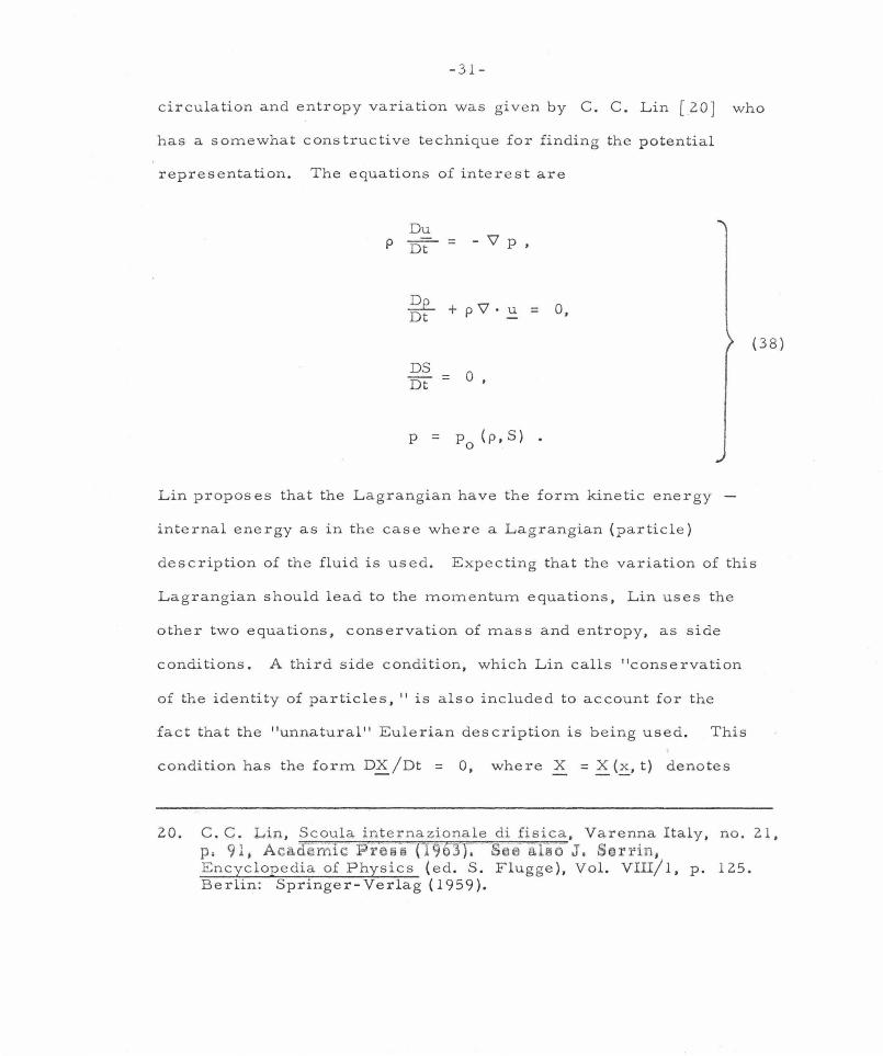
circulation and entropy variation was given by C. C. Lin [20] who

has a somewhat constructive technique for finding the potential

representation. The equations of interest are

Du p Dt = - \1 p I

gt + p \1. u = 0,

( 38)

DS 0 1 Dt =

p = Po (p, S)

Lin proposes that the Lagrangian have the form kinetic energy

internal energy as in the case where a Lagrangian (particle)

description of the fluid is used. Expecting that the variation of this

Lagrangian should lead to the momentum equations, Lin uses the

other two equations, conservation of mass and entropy, as side

conditions. A third side condition, which Lin calls "conservation

of the identity of particles," is also included to account for the

fact that the "unnatural" Eulerian description is being used. This

condition has the form DX /Dt = 0, where X = X (~, t) denotes

20. C. C. Lin, Scoula internazionale di fisica, Varenna Italy, no. 21, P• 91, Aea.dTmic-~r€u;a {1961)": Scul- also J, Sarrin, Encyclopedia of Physics ( ed. S. Flugge ), Vol. VIII/ 1, p. 125. Berlin: Springer- Verlag ( 1959 ).

-32-

the initial position of the particle which is at position x at time t,

The side conditions can be built into the variational principle by

using Lagrange multipliers. The resulting variational principle

has the form

oJJIL+p(pt+\l· (p~))- pl3 g~ - py· ~; j dxdt = o,

(39)

where p, 13 , y are Lagrange multipliers ,

1 2 L = 2 p u - p E( p, S)

and E(p, S) is the specific internal energy. The independent

variations of ~· p, S, X then lead to Euler equations which can

be put in the form

u = \l p + l3 \lS + \lX · y ,

h - (p + 1 2

= 13 st + Y. xt + 2 u ) t (40)

~ Dt = Es = T,

Dy 0 ' Dt =

where h = E + pj p 1s the enthalpy and use has been made of the

thermodynamic equation

-33-

[oE(p, S)J = p(p, S)

ap s P2

A direct calculation shows that the mom e ntum equations follow from

the set (40) . Herivel [ 21] gives the formulation in (39) and (40)

without the condition DX /Dt = 0. He arrives at the velocity

representation ~ = Vp + !3 '\1 S and notes that it is a particular

case of the form u = "V p + a '\1 !3 given by Clebsch [ 22] .

Although Herivel's representation does allow for some rotational

flows , in cases of uniform entropy only potential flows are

represented. It was this restriction which Lin [ 23 ] wanted to

overcome when he added the third side condition DX /Dt = 0 to

the variational principl e ( 39) . In the mo r e general representation

u = "Vp + !3 '\IS+ '\IX · y

which results, the term !3 '\1 S leads to vorticity due to entropy

variation and the three terms '\IX · y account for other sources of

rotation.

It can be shown that the Lin formulation goe s through with

only a single equation as the third side condi tion . That is, when

the scalar side condition DX /Dt = 0 is used in place of DX / Dt = 0

21. J . W. Herivel , Proc. Cambridge Phil. Soc . , Vol. 51 {1955) pp. 344-349 .

22. Loc . cit .

23. Loc. cit.

-34-

1n (39), with a scalar Lagrange multiplier y, the expression for

the velocity in (40) becomes

u = 'Vp + l3'VS + y'VX. ( 41)

The rest of the equations in (40) remain unchanged and the

momentum equations still follow.

An alternate view of Lin 1 s formulation can be taken in which

the side conditions are eliminated from the variational principle.

For this approach one begins by assuming the first two equations

in (40) as representations for ~ and p. Instead of using these

equations as they stand, the more conc1se expression for ~ given

in ( 41) is used and the notation for the potentials is changed so

that the representation is assumed in the form

u = \JfJ + a. 'Vl3 + s'V 11 •

s = S 1 ( 42)

where E is a known function which satisfies 2.

p E (p,S) = p (p,S). p 0

From equations (38), it follows that the potentials p, a., !3, £,11

must satisfy the equations

-35-

Da 0 Dt =

~ Dt = 0

QS. = 0 (43) Dt

l22l Dt = -E~

Qe +p\7 · ~ Dt = 0 ,

where u stands for the expression in (42). The set (43) follows

from varying p, a , f3 , ~ . Tl in the variational principle

where again th e Lagrangian density is the pressure. The variation

of p in (44) gives the equation of state p = p (p, S). This 0

variational formulation includes the formulations of Clebsch and

Bateman described earlier in this section.

Two important ideas which appear in the general fluid

formulation and will be used for finding variational formulations

for the examples which follow are: (i) use a velocity representation

of the form

""a. \l f3. L-J l l

i

-36-

where pairs of potentials a.., j3. are used for the different sources 1 1

of vorticity in the problem ; (ii) the Lagrangian density 1s the

pres sure suitably expressed 1n terms of the potentials.

-37-

7 . V a riational Princip l e s for Ro ssby Wave s 1n a S h allow B as i n a nd i n the "f3-Pla n e " Mode l

Rossby waves , also calle d plane tary waves , provide an

example of wave motion whose existence depends explicitly on the

rotation of a fluid . To give some idea of the phy sical si g nificance

of these waves , we will br i efly note some results of past

investi g ations . Plane tary waves were first found by Laplace and

Hough in their work on the theory of tides . Hough [ 24] s hows

that the small oscillations of a thin layer of fluid on a rotating

sphere under the action of gravitational and Coriolis forces , are

divided into two classes. The first are the usual gravity waves

modified to some extent by the rotation . The others , called

"oscillations of the second class" by Hough, are distinguished

from g ravity waves by the properties that their frequency is less

than twice the angular frequency rl of the sphere and is proportional

to rl in the limi t rl - 0. Ros sby [25 J shows that these second-

class oscillations are important in the theory of atmosphere flow.

He was able to isolate the second-class modes by considering

horizontal nondivergen t flow in a coordinate system which roughly

approximates a spherical globe. By means of this so-called

"f3-plane" model, Rossby gave the first clear physical

interpretation of these waves: the northward displacement of a

24. S.S. Hough , Phil. Trans .A, Vol. 191 ( 1898), pp. 139-185 .

25 . C . G . Rossby, J. Mar. Res . ,Vol. 2 ( 1939), pp. 38 - 55.

-38-

fluid element gives rise to a restoring force due to the increase in

the vertical component of angular velocity. Extensions of Rossby's

model were made by Haurwitz [ 26], and more recently by

Longuet-Higgins [ 27], who also studies the validity of the f) -plane

approximation.

Ros sby waves can also occur in rotating basins of variable

depth. Lamb [ 28] shows that slow second-class oscillations are

included in the solutions of the linearized shallow water equations

when applied to a rotating basin. For the special basin whose

depth is proportional to its radius squared, Phillips [ 29] finds that

the solution of Lamb's equations is expressible in terms of

elementary functions and that for low frequencies the dispersion

relation is similar to the one for Rossby waves in the f)-plane.

As regards finding a variational formulation for Rossby

waves, it is convenient to begin with the shallow basin model. A

variational principle is first given for the shallow water equations.

Then the rotation is put in by changing to a coordinate system

rotating with the fluid. The transformed equations and variational

principle are applicable to Rossby waves . Finally, by noting the

26. B. Haurwitz, J. Mar. Res., Vol. 3 (1940), pp. 35 -50.

27. M.S. Longuet-Higgins, Proc. Roy . Soc. A, Vol. 279 (1964), pp. 446-473. Proc. Roy. Soc. A, Vol. (1965), pp. 40-68.

28. Loc. cit. p. 326.

29 . N.A. Phillips, Tellus, Vol. XVII (1965), pp. 295-301.

-39-

similarity between the 13-plane equations for Rossby waves and

the rotating shallow water equations, a variational formulation

of the 13-plane model is given.

The shallow water equations written in cylindrical polar

coordinates ( r, g) are

+ 1

\ ru {h + 11) I r + ~~v(h+11)lg 0, 11t = r

vu9

2 + +

v ut uu --- = - g11r r r r

(45)

vv9

+ uv

+ 1

vt + uv = g 11g r r r r

where (u, v) are the velocity components of the fluid in the

directions (r, G), 11 is the free surface elevation and h is depth

of the bottom. A variational formulation for these equations is

found by applying the ideas discussed in the previous section. The

last two equations in ( 45) look like momentum equations for an

incompressible flow with pres sure g 11· Accordingly, the Clebs ch

type representation (see Section 6)

u = Pr + al3 r

1 <Pg a 13g) ( 46) v = + r

g11 = -j /Jt + a 13t + .!.(u2 2

+ v2) I

-40-

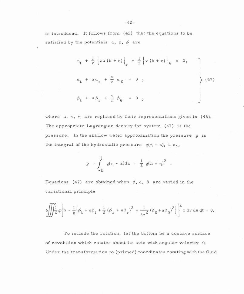
1s introduced. It follows from ( 45) that the equations to be

satisfied by the potentials a, 13, p are

1 'lt + r

ua r = 0 )

= 0 )

=

(47)

where u, v, '1 are replaced by their representations given in (46).

The appropriate Lagrangian density for system (47) is the

pressure. In the shallow water approximation the pressure p is

the integral of the hydrostatic pressure g (ij - z), i.e.,

'1

p = J g( '1 - z)dz = ~ g(h + i])2

.

-h

Equations (47) are obtained when p, a, 13 are varied in the

variational principle

To include the rotation, let the bottom be a concave surface

of revolution which rotates about its axis with angular velocity Q.

Under the transformation to (primed) coordinates rotating with the fluid

-41-

I I

u = u v = v - S";lr

r22r2 r22r 2 I I

T] = T] - 2g h = h + 2g ( 48)

Ql I I = Q - s-2 t t = t, r = r ,

the shallow water equations ( 45) become

1 I ru ( h + 11) I r +l. I v(h + ,) I Q 0 , T] +- = t r r

vu9

2 v

-2s-;Jv {49) ut + uv +-- = - gT]r, r r r

vv9 +~ + + 2r2u

1 vt +-- uv = g 'llg , r r r r

where the primes have been dropped and now u, v are the radial

and axial components of the velocity in a frame (r, 9) rotating

with the fluid; 11 is the free surface elevation above the

undisturbed surface s-22

r2 /2g and h is the depth of the basin

below the undisturbed free surface. When linearized, equations

(49) contain Rossby wave solutions. A variational formulation

for this system is found by using the modified representation [ 30]

30. For clarity, primes are kept on the potentials which represent the variables in the rotating frame.

-42-

PI I I

u = + a. f3 ' r r

1 (p~ I I

v = + a. f3g) - Or (50) r

-I p~ I I 1 (u2+v2)l gY) = + a. f3t + 2

( _,(I I (.\ I From 49) it follows that the equations to be satisfied by p , a. , ~'-'

are the same as equations (47) provided that u, v, '1 stand for

their new expressions in (50). These equations for the primed

potentials still come from varying the integral of the pressure

which now has the form

Dis regarding for the moment that the variables in equations ( 45)

and (49) stand for different quantities, we note that equations

( 45) are identical to equations ( 49) when the Coriolis terms are

added. Moreover, the complete variational formulation of ( 49)

is obtained from the formulation of ( 45) by only a minor change

(the term -Or in the expression for v) in the representation.

The equations for Rossby waves in an elementary

11 f3-plane 11 model are [31)

31. Loc. cit. Longuet-Higgins.

-43-

ut + uu + vu 2 n f(y) v = - px' X y

vt + uv + vv + 2 n f(y) u = - Py' (51) X y

u + v = 0 . X y

They are an attempt to locally approximate a thin shell of fluid

located between two concentric rotating spheres, by a flow between

two parallel planes. Thus, u, v are the velocity components of

the fluid in the directions of the rectangular coordinates x, y

which increase to the east and north respectively. The Coriolis

parameter 2 n f(y) is an approxima~ion to the true one 2 n cos ~

in spherical coordinates which varies with the latitude angle ~.

Rossby [ 32] notes that this variation is small near the equator

and takes 2 Q f'(y) = f3 a constant, in his model. Here, and in

the next paragraph, f3 is used as this constant of the "f3-plane''

model and should not be confused with the potential f3. ·

The last equation in {51) is satisfied identically when the

velocity {u, v) is derived from a stream function 4; by the

equations

u = - lj; • X

v =

32. Loc. cit.

-44-

Eliminating the pressure then leads to the equation

= 0.

It is interesting to observe that equation (52) has exact plane

wave solutions of the form ei(kx +my- wt); the nonlinear terms

cancel out. A uniform eastward flow can also be included so that

(52) has solutions of the form

ljJ = Uy - A cos my sin k (x - ct) ,

where

c =

Rossby considered the case m = 0 and noted that standing waves

occur at the critical wave number k = ~ Waves with s

wavelengths greater than 2iT/k move to the west, and shorter s

waves move to the east.

(52)

A variational principle for (52) would be most convenient

for studying Rossby waves . But, as ·it stands, not even the linear

terms in (52) are self-adjoint. By the substitution x = {,t

the linear terms become

-45-

which are self-adjoint and come from a variational principle of the

form

The nonlinear terms become

but in spite of the symmetry of the derivatives, they are not

self-adjoint and therefore cannot come from a variational principle

in terms of S,.

A variational formulation has been found for Rossby waves

in the f3-plane model by introducing a Clebsch-type representation.

Aside from the Coriolis terms, equations (51) are just

incompressible flow equations. As in the rotating basin problem,

the modification needed to include the Coriolis terms occurs when

a velocity corresponding to a vorticity equal to 20f(y) is

subtracted from the standard Clebsch representation. Accordingly,

either velocity representation

(i) (ii)

u = px +. a.f3 u = p + a.f3 + 2 0 F( y) X X X

or

v = p + a.f3 - 20xf(y) v = p + a.f3 • f(y) = Fl(y) y y y y

-46-

can be used along with

to obtain a variational formulation for (51). In either case the

Lagrangian density is the pressure and both sets of potentials

must satisfy equations of the form

ua. X

+ va. = y 0 I

!3t + u!3 + v!3 X y = 0 I

U + V = 0 1 X y

with u and v appropriately given by (i) or (ii).

Alternative forms of the above variational principles can

be given which lead to equations more suitable for linearization.

When the potentials are set to zero in (i) or (ii), fluid motion

remains. This motion is eliminated by transforming to new

potentials. In (ii), no motion corresponds to

p = 0, a.= 2 OF(y), !3 = - X •

Upon introducing the new potentials A, B by the equations

-47-

a. = A + ~ F(y), i3 = B - X~ '

representation (ii) can be written in the form

u = ~ + AB - A ~. X X

(53)

v = (!> + AB - B ~ f( y) ' y y

where

~ = ,6 + B ~f(y).

The expression for the pressure then becomes

p = I 1 2 2 l ?!>t + A Bt + 2 (u + v ) . (54)

The equations to be satisfied by ~. A, B are

(55)

u + v = 0) X y

-48-

where u, v stand for the expressions 1n (53). The set (55)

follows from the variation of ~. A, B in the pressure integral:

2l (~ +AB - .JZ.flA) 2

X X

-49-

8. The Variational Formulation for a Plasma

In the previous section variational formulations were found

for examples of fluid flow which contain rotation. The equations

of motion for such flows are complicated by the presence of

Coriolis terms of the form w x u. Variational formulations were

found for these equations by using a velocity representation obtained

by subtracting a velocity ..9. , such that w = curl ..9. , from

Clebsch-type representations. The equation of motion for a

charged particle moving in a magnetic field B will contain a

term B x ~ corresponding to the Lorentz force. In view of the

previous examples, it is expected that this term could be included

in a variational formulation by using a representation of the form

u = 'lp + a"Vf3 A

where A 1s the magnetic vector potential (i.e., B = curl A).

Using this idea we find a variational principle for the equations of

a gas which consists of several species of charged particles, when

the different species interact only through the electromagnetic

fields.

Let ui (~, t) and ni (~, t) be the Eulerian velocity and

number density of particles of species i which have mass m. 1

and charge e . . l

The equations to be assumed for the particles

in species i are the inviscid fluid equations:

m. 1

DS. 1

Dt

-50-

V'. u . -1

= 0 1

Du. -1

Dt + e .

1

c B Xu,

-1,

= 0 ,

(n., S . ) 1 1

= e. E -1-

1 V' p.

n. 1 1

no summation is implied by repeated subscripts. Although the

(56)

pressure terms in (56) can often be neglected in plasma problems,

as in the case of the so-called "collisionless" plasma, the terms

p . . will be included here since the variational formulation ·goes 1

through without extra difficulty. The electric and magnetic fields

satisfy the Maxwell equations

'V·B = 0,

'V· E = 4rr I: i

'YxE + 1

Bt c

V'xB-_!_E c -t =

e. n. 1 1

= 0 I

4rr ~ c L.....

i e.n.u.

1 1-l

(57)

-51-

Hopefully , as with the previous examples , having a variational

formulation for these general equations will help in finding

variational principles for the model equations which arise in

specific problems.

A variational principle for equations (56) and (57) 1s

found by representing the variables u .• -1

of the potentials f;. , l

f3. • £. • TJ· • A, l l l

u. = "Vp5. +a. . "Vf3. + £ . "YTJ. -1 1 1 1 1 1

e. l

m . 1

S. = £. 1 1

{ a f;. -n+ ~ 8;_(ni' £) + a/+ p . = +m. 1 1 1 1

S . , p., E, B 1n terms l l - -

via the equations

a f3. 8 ~; 1 z J j 1 a. . at + ;i at+ 2 ~i 1

where each e. 1S a known function which satisfies 1

2 n.

1

a§. 1

an.-1

(n . ,S . ) = 1 1

The representations in (5 8) for

(n., S.) 1 1

u. , S . and p. are similar to -1 1 1

the inviscid fluid case at the end of Section 6. The term e.

(58)

1

mi

like''

A now in the expression for u . accounts for the "Coriolis-- -1

e. term -

1 B xu. and the term - n.e. ljJ contributes to the

c -1 1 1

electric force e. E . From (56) and (57) it follows that the 1-

equations to be satisfied by the potentials are

-52-

'V· E = 4'1T L: e.n. i 1 1

'VxB l_E 4'1T L: - = c -t c i

Dn. 1

Dt + ni 'V· u. -1

= 0

Du . 1

Dt = O

Df3 . 1 = 0

Dt

D£. 1

Dt = O

DT) . 1

Dt = a e.

1 -~ (n., £.)

u ':>· 1 1 1

e.n.u. 1 1-1

The set {59) follows from varying the potentials

Si' lli' A, lj; in the variational principle

~-. 1 f3. ,

1

where E, B and the p. stand for the e,xpressions 1n {58). The -- 1

(59)

( 60)

variation of the n . leads to the equations of state p. = p (n., S . ). 1 1 0 . 1 1

1

-53-

9. Variational Principles for the Internal Waves of a Stratified Fluid

Another exam.ple of wave motion in a rotational fluid flow is

provided by the internal waves of a stratified fluid. If a vertical

gravitational force - p g~, (~ a unit vector in the z-direction) is

included in the equations of motion of a general compressible fluid

(32), new vertical gradients of the variables, density, pressure

etc., will appear. The gravitational force stratifies fluid in the

undisturbed state into horizontal layers of constant density. In an

analysis of the internal waves which can occur the density p ( z) 0

of the undisturbed layers is specified and model equations for the

perturbing motion are prescribed. Perhaps the simplest

formulation of internal waves is to consider motion of the interface

between two incompressible fluids of different density. In the

ocean, variation in salt concentration enables a continuous

stratification into vertical layers by the gravitational field.

Internal waves in a continuously stratified fluid are more easily

studied when the Bousinesq approximation is made. This consists

of isolating the internal waves from the compressional waves by

treating the fluid as incompressible. The equations for internal

waves in the Bousinesq approximation are

Du p Dt = -\1 p - g k ,

.Qe_ = 0 Dt '

(61}

'ii'·u= 0,

-54-

where p is no longer a given function of p, S and initially

p = p ( z) • 0

Long [ 33] treats equations ( 61) for the case of two-

dimensional steady motion in which ~ = (u(x, z), 0, w(x, z)}. The

stream function lJ; is introduced and its equation is integrated

once. A variational principle is given for the integrated equation

in which lJ; is varied. This analysis rests on using an auxiliary

variable z0

(1J;), which denotes the height of undisturbed

streamlines IJ;( z) = constant, and does not go through in the time

dependent case.

Variational formulations can be found for two- and three-

dimensional non-steady motions by using a more general (c;;lebsch-

type) representation. For equations ( 61) in two dimensions,

u = (u(x, z, t) , 0 , w(x, z , t)), we introduce the representation

u = ~X + af3 X

w = ~ + af3 z z ( 62)

p = p (a) 0

po(a)- Po( a) I ~t l 2 + w_2) + g z l . p = + af3t + 2 (u

where p (z) and p (z) are the equilibrium density and pressure 0 0

profiles. It can be shown that the quantities u, v, p, p given

33. R.R. Long, Tellus, vol. V, (1953). pp. 42-58.

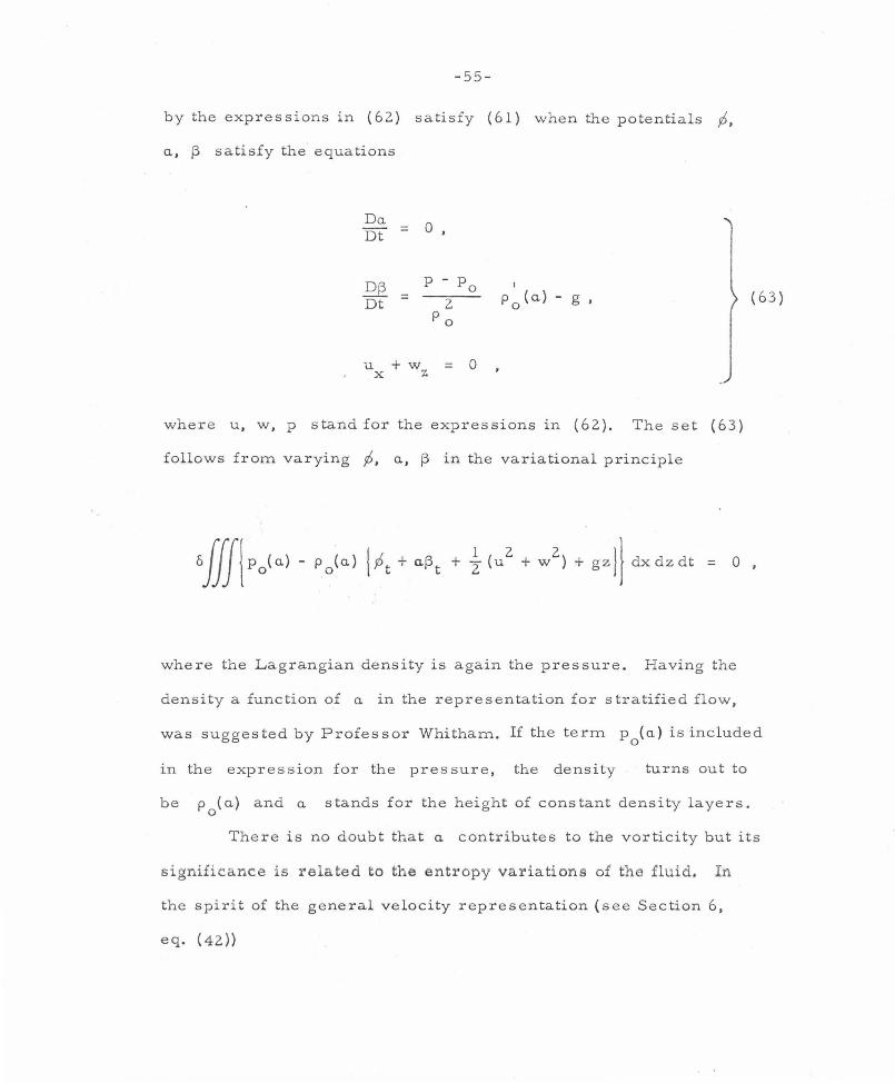
-55-

by the expressions in {62) satisfy (61) when the potentials p,

a., 13 satisfy the equations

Do. 0 • Dt =

~ p - Po 1

Dt = 2 p (a.) - g 0

(63)

Po

u + w'Z = 0 X

where u, w, p stand for the expressions in (62). The set (63)

follows from varying p, a., l3 in the variational principle

where the Lagrangian density is again the pressure. Having the

density a function of a. in the representation for stratified flow,

was suggested by Professor Whitham. If the term p0

(a.) is included

1n the expression for the pres sure, the density turns out to

be p {a.) and a. stands for the height of constant density layers. 0

There is no doubt that a. contributes to the vorticity but its

significance is related to the entropy variations o£ the .fluid. In

the spirit of the general velocity representation (see Section 6,

eq. (42))

-56-

( 64)

it would therefore be more appropriate to use the potentials ~. 11

in place of a., {3 for the velocity representation in a stratified

flow. Representation {62) differs from those previously given

because only three potentials a., {3, p are used to represent the

four functions u, v , p, p. The representation is therefore not

completely general and may not be capable of representing all

pas sible flows . This is more easily seen when ( 6 2) is

generalized to three dimensions by adding a second horizontal

velocity. Now equations {61) are being treated with

u = {u{x, y, z, t). v{x , y, z, t ). w{x, y, z , t)) . The natural

generalization of (62 ) is obtained by adding the equation

v = I> + a.{3 • y y

Now five variables are represented in terms of three potentials

and it is expected that some flows are omitted. This generality

question is best settled by the demands of specific problems.

For the last example we consider the variational

formulation of the equations for Rossby waves in a stratified fluid .

Combining equations {51) for the Rossby waves and equations (61)

for the internal waves , gives the equations

-57-

Du - f( y)v 1 Dt = -- px' p

Dv - f( y)u

1 Dt = py' p

(65)

Dw 1 Dt = pz - g ' p

~ = 0 V' • .::.:.... = 0 ' Dt '

where the velocity has components {u, v, w) in the directions

(x, y, z} which correspond to east-west, north-south and depth

coordinates respectively. The fluid flow described by (65)

has vorticity due to both the rotation of the Rossby waves and

the entropy variation of the internal waves . A velocity

representation of the form (64) is suggested in which a., f3

account for the Rossby wave effects and £, T) account for internal

wave effects . The desired representation has the form

u = !; + a.f3 + s T) - ~ a., X X X

v = P + a.f3 + s'l'1 - .J2fi: f(y) i3 y y y

w = !; + a.f3 + s'l'1 z ( 66) z z

p = p o( s>

p = Po(s) - Po(s) I Pt + 1 2. 2. 2. ) a.!3t + ST)t + 2 (u + v + w ) + gz

-58-

The equations to be satisfied by the potentials p, a, f3, £, 11 are

D a . r=;-;::;-Dt + '\J 2r2 f(y)v = 0

~- .JZii u= 0 Dt

QS. = 0 Dt

l2.!l p- Po I

Dt = 2 po(£)- g

Po

\l· u = 0

The set (67) follows from the variation of the five potentials

in the variational principle

(67)

0 .

-59-

APPENDIX A

The Singularity in K (x)

The kernel K (x) appropriate to water waves is given g

by the integral

· An estimate of K is obtained by writing g

l K (x) =

g 1T

l/2 [~tanh k h 0 J cos kx dk

where

1 =

1T

00

00 f .fi7k cos kx dk .. 0

+ f(x) ,

f(x) = ; ~ .Jilk /-I tanh k h0

- 1j cos kxdk.

(A-l}

(A-2}

l/2 The integral in (A- 2} can be evaluated and is equal to lz:!x I . The function f(x} is bounded by

-60-

co l £ I f(x) I $ .Jgfk ( l - >J tanh k h ) dk lT 0

co 4 £ < lT

Thus, for K (x) we have g

-2kh

~ 0 dk e =

l/2 Kg(x) = ~~I + f(x) ,

where

4 >Jg/2Tih 0

these formulas hold for all x.

4>Jg/2Tih 0

-61-

APPENDIX B

An Estimate of p(x, t) for a Breaking Wave

To help understand the effect of the singularity in K on g

breaking, we estimate the integral term p(x, t) for the singular

kernel

and a known breaking wave T)(x, t). Let

M 1(t) = max I 'llx(x, t) I X

M 2 (t) = max I 'llx)x, t) I X

The functions M1 (t) and M

2(t) will be determined later for a

specific breaking profile. An estimate of p(x, t) is obtained by

writing

co

p(x, t) = f IS ~-1/2 e- b IS I 'llxx(x- £, t) d£

-co

e -b Is I \ 'llx)x-£, t)

+ ·T) (x + £, t) I d£. XX

- 62-

Then

(B -1)

where the second mean value theorem was used toes timate the second

integral.

A breaking wave which is convenient for finding M 1

and

M2

1s provided by the solution of the equation

= 0

with 11 (x,O) = 11 (x) = - sinx. The solution to (B-2) is given 0

implicitly by the equations

from which the formulas

11x =

11xx =

l

{, =

I

110 ( {,)

I

X - ,., t ·10

,

+ 11 (t;,)t 0

11~ (S}

( l + 11~ (1~,)t) 3

(B- 2)

(B-3)

-63-

are derived. With these expressions for 11 and 11 viewed as X XX

functions of s and t, the lines sM on which l11x I is a maximum 1

at time t are found to be

= 2n'lT, n= 0, ± 1, ± 2, ... (B-4)

The lines sM on which l11xx I is a maximum at time t are found 2

from the equation

II 2 = 3t,.,

0

For the initial profile 11 (x} = - sin x, equation (B-5} becomes 0

which yields

2 t (cos SM ) 2

+ cos SM - 3t = 0 2 2

1 = 4t l- 1 ± ~1 + 24 t

2 ) .

To study the behavior near x = 0, (this behavior is repeated at

x = 2n'!T } we take n = 0 in (B-4) and the positive root in (B-6)

to ob tain

sM (t) = 0 , 1

12(t5-1)11/2 sM ( t) =

2 as t- 1

(B -5)

(B-6)

-64-

Substituting these values 1n (B-3) then gives

1

where tb(= 1) 1s the breaking time. Finally, by choosing

and using the above expressions for M1

and M2

in the bound

(B-1) we obtain