Asymptotics ofEigenpolynomials of

Exactly-Solvable OperatorsTanja Bergkvist

Department of MathematicsStockholm University

2007

Doctoral Dissertation 2007Department of MathematicsStockholm UniversitySE-106 91 Stockholm

Typeset by LATEXc©2007 by Tanja BergkvistISBN 91-7155-380-0Printed by US-AB, Stockholm 2007.

Summary

The main topic of this doctoral thesis is asymptotic properties ofzeros in polynomial families appearing as eigenfunctions to exactly-solvable differential operators (ES-operators). The study was ini-tially inspired by a number of striking results from computer exper-iments performed by G. Masson and B. Shapiro for a more restric-tive class of operators. Our research is also motivated by a classi-cal question going back to S. Bochner on a general classification ofdifferential operators possessing an infinite sequence of orthogonaleigenpolynomials. In general however, the sequence of eigenpolyno-mials of an ES-operator does not constitute an orthogonal systemand it can therefore not be studied by means of the extensive theoryknown for such systems. Our study can thus be considered as thefirst step to a natural generalization of the asymptotic behaviourof the roots of classical orthogonal polynomials. Also, many spe-cial functions appear as solutions to certain second-order differentialequations and hence solutions to exactly-solvable differential equa-tions might be thought of as higher order special functions. Ourmain definition is as follows. An exactly-solvable operator oforder k is a linear differential operator of the form

T =

k∑

j=1

Qj(z)dj

dzj

where the Qj are complex polynomials in one variable satisfyingthe condition degQj ≤ j with equality for at least one j. Weare interested in the sequence of polynomials pn∞n=0 satisfyingT (pn) = λnpn where deg pn = n, and λn is the spectral parameter.One can show that for all sufficiently large integers n there exists aunique and monic pn for any T as above. If degQk = k for the lead-ing term then T is called a non-degenerate ES-operator, whereasif degQk < k we call T a degenerate ES-operator. The majordifference between these two classes is that in the non-degeneratecase the union of all roots of all pn is contained in a compact set,as opposed to the degenerate case where the largest modulus of theroots of pn tends to infinity when n → ∞. Computer experimentsindicate that roots of eigenpolynomials of ES-operators fill piece-wise real analytic curves in the complex plane. One of the maintechnical tools in this thesis is the Cauchy transform of a probabil-

ity measure, which in the considered situation satisfies an algebraicequation - in the degenerate case however only after an appropriatescaling of the eigenpolynomials. Due to the connection between the(asymptotic) root measure and its Cauchy transform it is thus pos-sible to obtain detailed information on the limiting zero distribution.

Some Remarks. Let us mention some interesting but still un-exploited connections of our results to other fascinating fields:

1. The existence of a probability measure µ with compact sup-port such that its Cauchy transform satisfies an algebraic equationimplies that the Cauchy transform also satisfies a differential equa-tion (of order at most k) expressed by a so called Fuchsian operatorin the Weyl algebra A1(z, ∂). It is an open problem to determinethe class of all Fuchsian operators which arise via the limiting rootmeasure of eigenpolynomials associated to degenerate ES-operators.

2. In many situations considered in this thesis the support ofthe limiting root measure is a curvilinear tree in the complex planewhich can be straightened out in a certain canonical holomorphiccoordinate. The resulting usual tree has only a finite number ofpossible angles between its edges. This bears a strong resemblancewith the notion of amoeba in tropical algebraic geometry, which is anextremely active research area. But the actual connection betweenour ’generalized’ amoebas and the classical amoebas is unclear atthe moment.

3. The support of the limiting root measure seems to be a partof the global Stokes line of the associated ordinary linear differentialequation. But for orders k > 2 there is no satisfactory theory ofStokes lines, and the question about the exact interrelation betweenthe latter support and Stokes lines is still widely open.

4. In the non-degenerate situation considered in this thesis (seepaper I) it is only the leading coefficient of the differential equationwhich effects the limiting zero distribution. To change the situationin such a way that the whole symbol of the differential operator willbe important one has to, instead of the usual spectral problem, con-sider its homogenized version where the polynomial coefficient Qj ismultiplied by λj

n where λn is the spectral parameter. This directionis at present pursued by J. Borcea, R. Bøgvad and B. Shapiro.

This thesis consists of five papers, all devoted to the study of zerosof eigenpolynomials of ES-operators.

Paper I: In this paper we study roots of polynomials arising aseigenfunctions to non-degenerate ES-operators. In this case theeigenvalue equation can be considered as a natural generalizationto higher orders of the Gauss hypergeometric equation

(z2 − 1)f ′′(z) + (az + b)f ′(z) + cf(z) = 0

to which (for certain choices of a, b and c) the classical orthogonalJacobi polynomials appear as solutions. But for orders k > 2 thesequence of eigenpolynomials is in general not an orthogonal sys-tem. The main result in this paper is a complete characterizationof the asymptotic distribution of zeros of the eigenpolynomial of anarbitrary non-degenerate ES-operator. We thus settle several of theconjectures stated by G. Masson and B. Shapiro in [4]. Namely, forany such operator, we construct the probability measure µn (we callthis the root measure) of its unique and monic eigenpolynomial pn

by placing a point mass of size 1/n at each zero of pn. We thenprove that µn converges (weakly) to a unique probability measureµ whose Cauchy transform satisfies the equation C(z)k = 1/Qk(z)for almost all z ∈ C. Thus the asymptotic zero distribution of pn

depends only on the leading polynomial Qk of T . Moreover, suppµ is a tree which contains all the zeros of Qk and is contained inthe convex hull of the zeros of Qk. The proof of these properties ofsupp µ depends heavily on Lemma 3 in section 3 due to H. Rullgard.

Paper II: In this paper we adress a classical question going backto S. Bochner and H.L. Krall. A system of orthogonal polynomialswhich also appear as eigenfunctions of some finite-order differentialoperator is called a Bochner-Krall system and the correspondingspectral operator a Bochner-Krall operator. It is an open problemto classify all Bochner-Krall systems - a complete classification isonly known for operators of order k ≤ 4. Here we use the resultsobtained in paper I to settle a special case of a general conjecturedescribing the leading terms of all Bochner-Krall operators. Namely,in [4] it is conjectured that the leading coefficient of any such op-erator is a power of a polynomial of degree at most 2. Our mainresult in this paper is an affirmative answer to this conjecture for

Bochner- Krall operators of Nevai type - that is operators for whichthe system of eigenpolynomials is orthogonal with respect to a mea-sure of the so called Nevai class.

Paper III: This paper is devoted to a study on the location of zerosof individual eigenpolynomials of a confluent hypergeometric opera-tor, which is the simplest example of a degenerate ES-operator. Theclassical Laguerre polynomials appear as a special case, and somewell-known results about these are recovered by yet another methodand generalized. We pay particular attention to hyperbolicity prop-erties of the eigenpolynomials of this operator.

Paper IV: In this paper we extend our previous study to asymptoticproperties of zeros of eigenpolynomials for arbitrary degenerate ES-operators. We prove that (as opposed to the non-degenerate case)the zeros of the unique and monic nth degree eigenpolynomial pn donot stay in a compact set as its degree tends to infinity. However,computer experiments indicate the existence of a limiting root mea-sure supported on a tree in this case too, but that it has compactsupport only after an appropriate scaling. The main achievement inthis paper is an explicit conjecture and partial results (lower bound)on the growth of the largest modulus of the roots of pn. This can beseen as a generalization of the asymptotic behaviour of the maximalroot for classical orthogonal polynomials appearing as eigenfunc-tions to degenerate ES-operators - our conjecture is confirmed byknown results when reduced to such systems. Namely, let T be adegenerate ES-operator of order k and denote by j0 the largest j forwhich degQj = j in T (note that j0 < k). Denote by rn the largestmodulus of the roots of pn. Then

limn→∞

rn

nd= cT where d := max

j∈[j0+1,k]

(j − j0

j − degQj

)

and where cT is a positive constant. Based on this conjecturewe introduce the properly scaled polynomial qn(z) = pn(ndz) forwhich the zeros are (conjecturally) contained in a compact set whenn→ ∞. In fact, our natural heuristic arguments (see section 3) showthat d as above is the only possible choice which results in a nicealgebraic equation satisfied by the Cauchy transform of the asymp-totic root measure of qn(z). From this equation we can conclude

which terms of T that are relevant for the limiting zero distributionof its eigenpolynomials. Numerical evidence clearly illustrates thatdistinct operators whose scaled eigenpolynomials satisfy the sameCauchy transform equation when n→ ∞ yield identical zero distri-butions. It is still an open problem to describe its support explicitly.

Finally, as in the non-degenerate case, operators of the type weconsider here occur in the theory of Bochner-Krall systems. By com-paring known results on orthogonal polynomials with results on theeigenpolynomials studied here, we believe it will be possible to gainnew insight into the nature of Bochner-Krall systems.

Paper V: In this paper we extend earlier results from paper IVby establishing a lower bound for the largest modulus of the rootsof the eigenpolynomial of an arbitrary degenerate ES-operator. Wethus confirm the lower-bound part of our main conjecture as statedin paper IV.

Acknowledgements

First I would like to thank my dear PhD advisor Professor BorisShapiro for introducing me to this very fascinating and fruitful prob-lem. Without him this thesis would never have come into being. Oneof his first comments a few weeks after I had entered the Depart-ment of Mathematics at Stockholm University was: “You resemblean electron - you are everywhere at the same time!”, and I guess hemeant that my existence was like an overlap of wavefunctions thatnever would collapse - and he was right. The probablity for himto collapse as an effect of my intense nature was much higher (hementioned this several times) but in time we developed a fruitful col-laboration. I thank him for his professional guidance, his patience,kindness and support during my work.

I have had the pleasure to work with Hans Rullgard, who isone of the brightest persons I have ever met. His intelligence andimpressive intuition extends far beyond the field of mathematics andI thank him for many stimulating discussions.

I have also had the privilege to work with Professor Jan-ErikBjork who is one of the most knowledgeable and eccentric personsat the faculty. Professor Bjork is a person who can pick an arbitrarybook from the library and state the content of the theorem on page125, its originator and the year it was proved. I have learnt thehistory of mathematics and the life stories of its giants exclusivelyfrom my endless chats with Professor Bjork.

I am also indepted to Christian Gottlieb for guidance in my teach-ing and for his support and encouragement in this process.

It has been a pleasure to work with Johan Thorbiornson and ClasLofwall on the Internet based courses in mathematics. Thorbiornsonis one of the most optimistic and captivating mathematicians I havecollaborated with.

I would like to thank all PhD students for making my time at thedepartment pleasant and interesting. In particular my thoughts goto Veronica Crispin and Elin Ottergren for many wonderful momentswith joy and laughter, but also for their moral support in times ofsorrow. I will miss funny and crazy discussions enlightening the daywith my PhD student fellow Karl Rokaeus. Peas to my fellows inMatlaget.

I would like to express my gratitude to system administrator

Tomas Ericsson for immediate help in all situations and especiallyfor exchanging my keyboard when it collapsed from pieces of noodlesbeing stuck between the keys.

I am grateful to Barbro Fernstrom and Tom Wollecki for theirkindness and helpfulness in many practical situations. I must con-fess that during my years at the department I only emptied the dish-washer once - please do not consider this a feministic standpoint!I really have no sensible excuse but my occupation with roots ofeigenpolynomials.

The list of people I am indepted to could be made much longer. Iwould like to thank all employees at the Department of Mathematicsat Stockholm University. You have all been a source of inspirationto me. I am also deeply grateful to the staff at the Department ofMathematics at Lund University where I as a young student discov-ered the beauty of mathematics.

Finally I want to thank my family - my parents, grandparents,brother with family, and the most important person in my life: mydaughter Nadja - for their love and support.

My interest in natural science began with astronomy which wasmy main occupation as a teenager. Over time my focus passed tophysics until I finally realized one day that it’s all mathematics!Years of research in the field of mathematics has deeply affected myunderstanding of Nature. Nowadays, whenever I look up to the skyI can’t stop wondering if any of the constellations of stars I studiedas a youngster isn’t actually the distribution of zeros of a polynomialarising as an eigenfunction to an operator I haven’t yet considered.

I dedicate this thesis to my mother Anni and to my grandparentsSlavka and Nikola who are the reason I came this far and becamethe person I am today. You have been the main source of inspirationin my life - thank you for believing in me!

Tanja Bergkvist, February 2007

PAPER I

On Polynomial Eigenfunctions for aClass of Differential Operators

Tanja Bergkvist & Hans RullgardPublished in Mathematical Research Letters 9, 153-171 (2002)

AbstractIn this paper we study the asymptotic properties of ze-

ros of polynomials arising as eigenfunctions of a certainclass of operators (non-degenerate exactly-solvable opera-tors). We prove that when the degree of the unique andmonic eigenpolynomial tends to infinity, its zeros are dis-tributed according to a certain probability measure whichis compactly supported on a tree and which depends onlyon the leading term of the operator.

1 Introduction

Jacobi polynomials are solutions of the differential equation

(z2 − 1)f ′′(z) + (az + b)f ′(z) + cf(z) = 0, (1)

where a, b, c are constants satisfying a > b, a + b > 0 and c =n(1 − a − n) for some nonnegative integer n. It is a classical factthat the zeros of the Jacobi polynomials lie in the interval [−1, 1],

and that their density in this interval is proportional to 1/√

1 − |z|2in the limit when the degree n tends to infinity. The usual proof ofthis statement involves the observation that, for fixed a and b, theJacobi polynomials constitute an orthogonal system of polynomialswith respect to a certain weight function on the interval [−1, 1]. Thedesired conclusion then follows from the general theory of orthogonalsystems of polynomials.

The following appears to be a natural generalization of the dif-ferential equation (1). Let k ≥ 2 be an integer, and let Q0, . . . , Qk

be polynomials in one complex variable satisfying degQj ≤ j withequality when j = k. Moreover, we make a normalization by assum-ing that Qk is monic. Consider the differential operator

TQ(f) =

k∑

j=0

Qjf(j) (2)

1

where f (j) denotes the jth derivative of f . Operators of this typeappear for example in the theory of Bochner-Krall systems of orthog-onal polynomials, see [3]. This operator was studied by G. Massonand B. Shapiro in [4]. Particular attention was given the more spe-cial operators T ′(f) = Qkf

(k) and T ′′(f) = (d/dz)k (f(z)Qk(z)).These are indeed special cases of (2) obtained by taking Qj = 0 or

Qj =(

kj

)Q

(k−j)k respectively, for j = 0, . . . , k − 1. The following re-

sult, which shows that TQ has plenty of polynomial eigenfunctions,was proved for the operators T ′ and T ′′ in [4]:

Theorem 1 For all sufficiently large integers n there exists a uniqueconstant λn and a unique monic polynomial pn of degree n whichsatisfy

TQ(pn) = λnpn. (3)

Moreover, we have λn/n(n− 1) . . . (n− k + 1) → 1 when n→ ∞.

G. Masson and B. Shapiro made a number of striking conjectures,based on numerical evidence, about the zeros of the eigenpolynomi-als pn. They also observed that when k > 2, the sequence pn is ingeneral not an orthogonal system of polynomials, so it cannot bestudied by means of the extensive theory known for such systems.

The goal of this paper is to prove some of the conjectures in [4].More precisely, we shall show that in the limit when n→ ∞, the ze-ros of pn are distributed according to a certain probability measure.This probability measure depends only on the “leading polynomial”Qk and may be independently characterized in the following way.

Theorem 2 Let Qk be a monic polynomial of degree k. Then thereexists a unique probability measure µQk

with compact support whoseCauchy transform

C(z) =

∫dµQk

(ζ)

z − ζ(4)

satisfies C(z)k = 1/Qk(z) for almost all z ∈ C.

We record some properties of the measure µQkwhich will be en-

countered in the proof of Theorem 2. Let suppµ denote the support

2

of a measure µ. Also, let

Ψ(z) =

∫Qk(z)

−1/k dz

be a primitive function of Qk(z)−1/k. At this point, we think of

Ψ as a locally defined function in any simply connected domainwhere Qk does not vanish. The choice of a branch of Qk(z)

1/k andan integration constant is of no importance here. As need arises,specifications will be made concerning these choices.

Theorem 3 Let Qk and µQkbe as in Theorem 2. Then supp µQk

isthe union of finitely many smooth curve segments, and each of thesecurves is mapped to a straight line by the mapping Ψ. Moreover,suppµQk

contains all the zeros of Qk, is contained in the convex hullof the zeros of Qk and is connected and has connected complement.

If p is a polynomial of degree n, we can construct a probabilitymeasure µ by placing a point mass of size 1/n at each zero of p. Wewill call µ the root measure of p. Our main result is

Theorem 4 Let pn be the monic degree n eigenpolynomial of theoperator TQ and let µn be the root measure of pn. Then µn convergesweakly to µQk

when n→ ∞.

To illustrate, we show the zeros of the eigenpolynomial p40 forthe order 5 operator TQ with Q5(z) = z(z − 1 + i)(z − 5)(z − 2 −4i)(z − 4 − 4i) and Q0 = · · · = Q4 = 0. Large dots represent thezeros of Q5 (which are, in this case, also zeros of pn) and small dotsrepresent (the remaining) zeros of p40. It is remarkable how well thezeros of the eigenpolynomial line up along the curves predicted byour results. Notice also how these curves are straightened out bythe mapping Ψ, see Figure 1.

It is not difficult to deduce various other features of the measureµQk

from the properties given in Theorem 3 and the defining prop-erty (4). For example, a recipe for computing the angles betweenthe different curve segments is conjectured in [4]. The correctness ofthe procedure follows easily from our results. We refrain from goinginto details, but the key observation is the following. Suppose z0 is

3

Figure 1: Zeros of the polynomial Q5 and the eigenpolynomial p40 (left) andthe image of these zeros under a branch of the mapping Ψ.

a point on one of the curve segments in suppµQkand let C1 and C2

be the limiting values of C(z) as z approaches z0 from different sidesof the curve. Then C1 and C2 are kth roots of 1/Qk(z0), and theiractual values are easily found if the combinatorics of suppµQk

areknown (which was assumed in the recipe mentioned above). Fromthe fact that πµQk

= ∂C/∂z ≥ 0, it follows that the curve must beperpendicular to C1 − C2 at z0. Using this observation where sev-eral curves meet, it is possible to deduce the angles between them.Notice also that the density of µQk

at z0 is proportional to |C1−C2|.

It is particularly easy to compute µQkwhen Qk has only real zeros.

Namely, denote the zeros by z1, . . . , zk in increasing order. FromTheorem 3 we know that supp µQk

= [z1, zk]. A direct computationshows that on the subinterval [zj , zj+1], the measure is given by

µQk=

1

π

∂C

∂z=

2

π|Qk|1/ksin

(πj

k

)dx

where dx denotes Lebesgue measure on the real line. This remainstrue even if Qk has multiple zeros, except if all the zeros coincide.In this case, µQk

reduces, of course, to a point mass at this multiplezero.

Let us finally discuss some possible applications and directionsfor further research. As we already mentioned, operators of thetype we consider occur in the theory of Bockner-Krall orthogonal

4

systems. More precisely, a Bochner-Krall system (BKS), is a se-quence of polynomials pn which are both eigenpolynomials of anoperator TQ (here one omits the assumption that degQk = k) andalso orthogonal with respect to a suitable inner product. It is a longstanding problem to classify all BKS. A great deal is known aboutthe asymptotic distribution of zeros of orthogonal polynomials. Bycomparing such results with our results on the distribution of zerosof eigenpolynomials, we believe that it will be possible to gain newinsight into the nature of BKS. To get the most out of this approach,however, it would be desirable to have generalizations of our resultsto the case degQk < k. Computer experiments performed by thefirst author indicate that a limiting measure exists in this case too,but that it may not have compact support.

This paper is organized as follows. In section 2 we compute thematrix for the operator TQ with respect to the basis of monomials1, z, z2, . . ., and use this to prove Theorem 1 for an arbitrary op-erator of the type we consider. Section 3 contains a proof of theuniqueness part of Theorem 2. Along the way, we also prove es-sentially all the statements in Theorem 3. In section 4 we recallsome basic facts on the weak topology of measures in the complexplane and on logarithmic potentials and Cauchy transforms. Wealso outline the connection of these concepts to root measures ofpolynomials and prove a general result on the relation between thezeros of a polynomial and those of its derivative. In the final section5 we apply the ideas from the previous section to give a proof ofTheorem 4. The existence part of Theorem 2 is also a consequenceof this proof.

Acknowledgements. The authors are sincerely grateful to HaroldShapiro for highly valuable comments and discussions, and in par-ticular for suggesting the use of the Cauchy transform. We wouldalso like to thank Gisli Masson and Boris Shapiro for introducing usto the problem and for their support during our work.

5

2 Calculation of the matrix

Proof of Theorem 1. We now prove that Theorem 1 as stated inIntroduction holds for any operator of the type we consider. Recallthat the differential operator TQ is defined by

TQ = Qkdk

dzk+Qk−1

dk−1

dzk−1+ · · ·+Q1

d

dz+Q0

where the Qm are polynomials such that degQm ≤ m for m =0, . . . , k and degQk = k. Let pn(z) =

∑ni=0 an,iz

i be a monic poly-nomial of degree n and let Qm(z) =

∑mj=0 qm,jz

j . Using these nota-tions we get

TQ(pn) =k∑

m=0

Qm · dm

dzmpn =

k∑

m=0

[ m∑

j=0

qm,jzj

]·[ n∑

i≥m

an,i ·i!

(i−m)!zi−m

]

=k∑

m=0

n∑

s=0

[ ∑

s=j+i−mm≤i≤n0≤j≤m

qm,j · an,i ·i!

(i−m)!

]zs

=n∑

s=0

[ k∑

m=0

∑

s=j+i−mm≤i≤n0≤j≤m

qm,j · an,i ·i!

(i−m)!

]zs.

Lemma 1 If pn is monic and TQ(pn) = λnpn then

λn =k∑

m=0

qm,m · n!

(n−m)!.

Proof. With pn monic and TQ(pn) = λn·pn = λnzn+λn·an,n−1z

n−1+. . .+λn ·an,0, finding the eigenvalue λn amounts to finding the coef-ficient at zn in TQ(pn). Note that deg

(Qm

dm

dzmpn

)≤ m+ n−m = n

with equality if and only if degQm = m. Thus we can assume thatpn = zn since any lower degree terms of pn will result in terms ofdegree lower than n in TQ(pn). Thus

6

TQ(zn) =

k∑

m=0

Qm · dm

dzmzn =

k∑

m=0

Qm · n!

(n−m)!zn−m

=k∑

m=0

[( m∑

j=0

qm,jzj

)· n!

(n−m)!zn−m

]

=k∑

m=0

[ m∑

j=0

qm,j ·n!

(n−m)!zj+n−m

].

Setting j = m we get

λnzn =

k∑

m=0

qm,m · n!

(n−m)!zn =⇒ λn =

k∑

m=0

qm,m · n!

(n−m)!.

Lemma 2 For n ≥ 1 the coefficient vector X of pn with componentsan,0, . . . , an,n−1 satisfies the linear system MX = Y , where Y isa vector and M is an upper triangular matrix, both with entriesexpressible in the coefficients qm,j.

Proof. The relationTQ(pn) = λn · pn

is equivalent to

n∑

s=0

[ k∑

m=0

∑

s=j+i−mm≤i≤n0≤j≤m

qm,j · an,i ·i!

(i−m)!

]zs = λn

n∑

s=0

an,szs.

With j = m + s − i the condition j ≤ m gives i ≥ s and thecondition j ≥ 0 results in m ≥ i − s. Therefore the above systemwill be equivalent to

n∑

s=0

[ ∑

s≤i≤n

∑

i−s≤m≤min(i,k)

qm,m+s−i ·i!

(i−m)!· an,i −λn · an,s

]zs = 0.

Thus for each s we have∑

s≤i≤n

∑

i−s≤m≤min(i,k)

qm,m+s−i ·i!

(i−m)!· an,i − λn · an,s = 0

7

or, equivalently,

∑

s≤i≤n−1

∑

i−s≤m≤min(i,k)

qm,m+s−i ·i!

(i−m)!· an,i − λn · an,s =

=∑

n−s≤m≤min(n,k)

qm,m+s−n · n!

(n−m)!· an,n

where an,n = 1. The n × n matrix M is thus constructed for 0 ≤s ≤ n − 1 and 0 ≤ i ≤ n − 1. The left-hand side of the aboveequation corresponds to the (s + 1)st row in M multiplied by thecolumn vector X, and the right-hand side represents the (s + 1)strow in Y . Thus the entries of M are given by

Ms+1,i+1 =∑

i−s≤m≤min(i,k)

qm,m+s−i ·i!

(i−m)!− λn · δi,s (5)

where δ denotes the Kronecker delta. The condition i ≥ s impliesthat M is upper triangular.

We can now prove Theorem 1. Using Lemma 1 we get

λn

n(n− 1) . . . (n− k + 1)=

∑km=0 qm,m · n!

(n−m)!

n(n− 1) . . . (n− k + 1)

=q0,0

n!n!

+ q1,1n!

(n−1)!+ q2,2

n!(n−2)!

+ . . .+ qk−1,k−1n!

(n−k+1)!+ qk,k

n!(n−k)!

n(n− 1) . . . (n− k + 1)

=q0,0

n(n− 1) . . . (n− k + 1)+

q1,1

(n− 1) . . . (n− k + 1)+ . . .

. . .+qk−1,k−1

(n− k + 1)+ qk,k.

Thus

limn→∞

λn

n(n− 1) . . . (n− k + 1)= qk,k = 1,

and the first part of Theorem 1 is proved. To prove the uniquenesspart, we show that the determinant of the matrix M constructed inLemma 2 is nonzero for all sufficiently large n. Since the matrix isupper triangular its determinant equals the product of the diagonalelements. Thus it suffices to prove that for sufficiently large n everydiagonal element is nonzero.

8

The diagonal element Mi+1,i+1 of M is obtained by letting i = s in(5) and so

Mi+1,i+1 =∑

0≤m≤min(i,k)

qm,m · i!

(i−m)!− λn

for i = 0, . . . , n− 1. But the last expression equals λi − λn. Indeed,if i ≥ k then

∑

0≤m≤min(i,k)

qm,m · i!

(i−m)!=

∑

0≤m≤k

qm,m · i!

(i−m)!= λi.

If i < k then this is again true since by definition i!/(i −m)! = 0for i < m ≤ k. Thus we have to show that λi − λn 6= 0 ∀i < nas n → ∞. For small values of i (i < k) we have λi < ∞ butλn → ∞ as n → ∞, implying λi − λn 6= 0. For larger values of i(0 < m < k ≤ i) we get

λn − λi =

k∑

m=0

qm,mn!

(n−m)!−

k∑

m=0

qm,mi!

(i−m)!

=k∑

m=0

qm,m

[n!

(n−m)!− i!

(i−m)!

].

Dividing the last expression by n!(n−k)!

− i!(i−k)!

we obtain

λn − λi

n!(n−k)!

− i!(i−k)!

= qk,k +

k−1∑

m=1

qm,m

n!(n−m)!

− i!(i−m)!

n!(n−k)!

− i!(i−k)!

.

which tends to qk,k = 1 as n→ ∞, since for each m ≤ k − 1 we get

limn→∞

n!(n−m)!

− i!(i−m)!

n!(n−k)!

− i!(i−k)!

= limn→∞

i!(n−m)!

(n!i!− (n−m)!

(i−m)!

)

i!(n−k)!

(n!i!− (n−k)!

(i−k)!

)

= limn→∞

(n− k)!

(n−m)!·(

n!i!− (n−m)!

(i−m)!

)(

n!i!− (n−k)!

(i−k)!

)

= 0.

Therefore λn − λi 6= 0. Thus, as n→ ∞, every diagonal element ofM becomes nonzero so M is invertible and the systemMX = Y hasa unique solution.

9

3 Probability measures whose Cauchy transformsatisfies an algebraic equation

In this section we will prove the uniqueness part of Theorem 2 andshow that the measure µQk

, if it exists, has the properties stated inTheorem 3. The proof relies heavily on the following lemma.

Lemma 3 Let A ⊂ C be a finite set, U ⊂ C a convex domainand χ : U → A a measurable function such that ∂χ/∂z ≥ 0 (inthe sense of distributions). Let a ∈ A, z0 ∈ U and assume thatχ−1(a) ∩ |z − z0| < r has positive Lebesgue measure for everyr > 0. Then χ(z) = a almost everywhere in U ∩ (z0 + Γa) where

Γa = z ∈ C; Re(az) ≥ Re(bz), ∀b ∈ A. (6)

Note that if χ−1(a)∩|z−z0| < r has positive Lebesgue measurefor every a ∈ A and all r > 0, then χ is determined completely (out-side a set of measure 0) since the cones Γa cover the whole complexplane.

Proof. Let χa denote the characteristic function of the set χ−1(a).We will show that if z1, z2 ∈ U with z2 − z1 ∈ Γa, and φ is a pos-itive test function such that z1 + supp φ and z2 + supp φ are bothcontained in U , then

(φ ∗ χa)(z1) ≤ (φ ∗ χa)(z2). (7)

The desired conclusion follows from this. Indeed, let φj be a se-quence of positive test functions such that suppφj → 0 and

∫φj dλ =

1, where λ denotes planar Lebesgue measure. We know then thatφj ∗ χa converges in L1

loc to χa. Hence, for any ǫ, r > 0 we can findfor all sufficiently large j a point z1 with |z1 − z0| < r such that(φj ∗ χa)(z1) > 1 − ǫ. It follows from (7) that (φj ∗ χa)(z2) > 1 − ǫand hence

|(φj ∗ χ)(z2) − a| =

∣∣∣∣∫φj(z2 − ζ)(χ(ζ)− a) dλ(ζ)

∣∣∣∣ < ǫmaxb∈A

|b− a|

for all z2 ∈ z1 + Γa. Letting ǫ and r tend to 0 and j → ∞ it followsthat χ(z) = limj→∞(φj ∗ χ)(z) = a for almost all z in z0 + Γa.

We now prove the inequality (7). Without loss of generality wemay assume that z2 − z1 > 0 and that a = 0, for the general case

10

can be reduced to this situation by replacing χ with the functioneiθ(χ(eiθz)−a) where θ = arg(z2−z1). The assumption that z2−z1 ∈Γa then implies that A is contained in the closed left half planeRe z ≤ 0.

For any ǫ > 0, let χǫ = log(χ− ǫ) where we have chosen a branchof the logarithm function which is continuous in the left half plane.Let ψ be a positive test function and note that ∂(ψ ∗χ)/∂z ≥ 0 andReψ ∗ χ ≤ 0. It follows that

Re∂

∂zlog(ψ ∗ χ− ǫ) = Re

(1

ψ ∗ χ− ǫ· ∂(ψ ∗ χ)

∂z

)≤ 0.

When suppψ → 0 with∫ψ dλ = 1, we have that log(ψ∗χ−ǫ) → χǫ

in L1loc, and hence as a distribution. By passing to the limit it follows

that

Re∂χǫ

∂z≤ 0.

If we write χǫ = σǫ + iτǫ, this means that

∂σǫ

∂x≤ ∂τǫ

∂y. (8)

Fix a positive test function φ such that zj + supp φ ⊂ U forj = 1, 2 and consider the function (φ∗σǫ)(z1 +ξ) of the real variableξ. It follows from (8) and the fact that τǫ is uniformly bounded forall ǫ that

∂

∂ξ(φ ∗ σǫ)(z1 + ξ) =

∫∂φ

∂x(z1 + ξ − ζ)σǫ(ζ) dλ(ζ)

≤∫∂φ

∂y(z1 + ξ − ζ)τǫ(ζ) dλ(ζ)

≤ M

where the constant M does not depend on ǫ. In particular,

(φ ∗ σǫ)(z2) − (φ ∗ σǫ)(z1) ≤M |z2 − z1|. (9)

On the other hand it is clear that

(φ ∗ σǫ)(z) = log ǫ · (φ ∗ χa)(z) +O(1). (10)

Now (7) follows from (9) and (10) when ǫ→ 0.

11

We deduce two corollaries of Lemma 3.

Corollary 1 Let U ⊂ C be a convex domain and A ⊂ C a finite set.If v is a subharmonic function defined in U such that 2∂v/∂z ∈ Aalmost everywhere, then v is convex.

Recall that a subharmonic function can locally be written as thesum of a harmonic function and a logarithmic potential. It followsthat the distribution ∂v/∂z is represented by a locally integrablefunction. The condition 2∂v/∂z ∈ A should be interpreted by say-ing that 2∂v/∂z is represented by a measurable function with valuesin A.

Proof. Let χ = 2∂v/∂z. Since v is subharmonic, ∂χ/∂z ≥ 0.Take any point z0 ∈ U and let A0 be the set of all a ∈ A suchthat χ−1(a) has positive measure in every neighbourhood of z0. LetU0 be a convex neighbourhood of z0 such that χ(z) ∈ A0 almosteverywhere in U0. By Lemma 3, χ(z) = a almost everywhere inU0 ∩ (z0 + Γa) where Γa is defined by (6) but with A0 in place of A.This implies that v(z) = v(z0)+Re a(z−z0) for all z ∈ U0∩(z0+Γa),so that

v(z) = v(z0) + maxa∈A0

Re a(z − z0), z ∈ U0.

We have shown that in a neighbourhood of z0, v is the maximumof certain linear functions, hence it is convex there. Since z0 wasarbitrary, it follows that v is convex.

Corollary 2 Let A ⊂ C be a finite set, U ⊂ C a convex domainand let χ : U → A be a measurable function. Then ∂χ/∂z ≥ 0 ifand only if there exist real numbers ca (possibly equal to −∞) suchthat χ(z) = a almost everywhere in Ga where

Ga = z ∈ U ; ca + Re(az) ≥ cb + Re(bz), ∀b ∈ A.

Proof. Suppose ca are real numbers such that χ(z) = a almosteverywhere in Ga. Let v(z) = maxa∈A (ca + Re(az)). Then v issubharmonic and χ = 2∂v/∂z, hence

∂χ

∂z= 2

∂2v

∂z∂z≥ 0.

12

Suppose conversely that ∂χ/∂z ≥ 0. Since ∂χ/∂z is real, thereexists a real valued function v defined in U with 2∂v/∂z = χ. Itfollows from Corollary 1 that v is convex. Moreover, we see fromthe proof that

v(z) = maxa∈A

(ca + Re(az))

whereca = inf

z∈U(v(z) − Re(az)).

If we define Ga using these constants ca it follows that v(z) = ca +Re(az) for z ∈ Ga, hence χ(z) = 2∂v/∂z = a in Ga.

Fix a monic polynomial Qk of degree k and suppose that µ is acompactly supported probability measure whose Cauchy transformC(z) satisfies

C(z)k = 1/Qk(z). (11)

We will first show that µ has the properties asserted in Theorem 3,except that supp µQk

is contained in the convex hull of the zeros ofQk, which will be proved in section 5.

Lemma 4 If the Cauchy transform of µ satisfies (11), then the sup-port of µ is the union of finitely many smooth curve segments. Thesecurves are mapped to lines by Ψ.

Proof. It is sufficient to prove that suppµ has these properties ina neighbourhood of any given point z0. Assume first that Qk(z0) 6=0. Choose a branch of Qk(z)

−1/k defined in a simply connectedneighbourhood of z0 and let Ψ be a primitive function of Qk(z)

−1/k.Let U be a convex neighbourhood of Ψ(z0) so small that Ψ mapsa neighbourhood of z0 bijectively onto U . By (11) we can writeC(z) = χ(Ψ(z))Qk(z)

−1/k for z ∈ Ψ−1(U), where χ has values inthe set of kth roots of unity. If we write w = Ψ(z), then

πµ =∂C

∂z=∂χ(Ψ(z))

∂z·Q−1/k

k = Ψ∗

(∂χ

∂w

)· ∂Ψ∂z

·Q−1/kk

= Ψ∗

(∂χ

∂w

)· |Qk|−2/k

where Ψ∗ denotes the pullback of distributions in U by Ψ. Since µis positive, it follows that

∂χ

∂w≥ 0.

13

By Corollary 2, U is the union of sets Ga whose boundaries arefinite unions of line segments, such that χ is constant in each Ga.It follows that supp µ ∩ Ψ−1(U) = Ψ−1(supp ∂χ/∂z) is the union offinitely many curve segments which are mapped to straight lines byΨ.

If z0 is a zero of Qk, we take a disc D centered at z0 wich doesnot contain any other zeros of Qk. If γ is any ray emanating at z0,we can define single valued branches of Q(z)−1/k and Ψ in D r γ.Notice that Ψ is continuous up to z0. Let U be any half disc centeredat Ψ(z0) and contained in Ψ(D r γ). It follows as in the first partof the proof that suppµ has the required properties in Ψ−1(U). Byvarying γ and U , we see that the same holds in a full neighbourhoodof z0.

Hence supp µ can be thought of as a graph whose edges are smoothcurve segments connecting certain vertices. The statement thatsuppµ is connected and has connected complement then means thatit is a connected graph without cycles, that is a tree. Recall that aconnected graph is a tree precisely if the number of vertices exceedsthe number of edges by exactly one.

Lemma 5 If the Cauchy transform of µ satisfies (11), then the sup-port of µ is a tree.

Proof. We will first prove that supp µ is connected. To do this wewill show that if U is a bounded domain which is connected andsimply connected, and the boundary of U does not intersect suppµ,then either supp µ ⊂ U or supp µ ⊂ C r U . From this it easilyfollows that supp µ is connected. Now it is clear that all the zerosof Qk are either contained in U or in the complement of U , sinceC(z) defines a continuous branch of Qk(z)

−1/k along ∂U . Observealso that

1

2πi

∫

∂U

C(z) dz =1

2πi

∫

C

∫

∂U

dz

z − ζdµ(ζ) =

∫

U

dµ(ζ). (12)

Now if all the zeros of Qk are contained in the complement of U ,there is an analytic continuation of C(z) across U , hence the lefthand side of (12) vanishes. It follows that suppµ ⊂ C r U . If onthe other hand, all the zeros of Qk are contained in U , then C(z)has an analytic continuation in CrU which is asymptotically equal

14

to a/z for some kth root of unity a when z → ∞. Thus the lefthand side of (12) is equal to a. Since the right hand side is positive,a must be 1, which means that all the mass of µ is in U . Hence wehave proved that suppµ is connected.

Now let E be the set of all curve segments in supp µ and let Vbe the set of vertices which are endpoints of the edges in E. Wemay assume that V contains all the zeros of Qk. To every paire ∈ E, v ∈ V such that v is an endpoint of e, we assign a numberν(e, v) by the following rule. Let γ be a small loop winding oncearound v in the clockwise direction, and let ν(e, v) be the jumpof (2πi)−1 logC(z) when z crosses e moving along γ. This number,which is defined modulo Z, will be uniquely determined if we requirethat 0 < ν(e, v) < 1. Assume now that v is not a zero of Qk andlet e1, . . . , er be the curves in E having v as one endpoint. (If somecurve has both its endpoints in v, it will be counted twice.) Selecta branch of Qk(z)

1/k near v and observe that by Lemma 3 and theproof of Lemma 4, Qk(z)

1/kC(z) is a kth root of unity, which movesonce around the unit circle in the counterclockwise direction as zmoves along γ. It follows that ν(e1, v) + · · · + ν(er, v) = 1. Ifinstead v is a zero of Qk of multiplicity m, a slight modification ofthe argument shows that ν(e1, v) + · · · + ν(er, v) = 1 − m/k. Onthe other hand, it is clear that ν(e, v1) + ν(e, v2) = 1 where v1, v2

are the endpoints of e ∈ E. Hence the sum of all the ν(e, v) is equalboth to ♯V − 1 and to ♯E. Since suppµ is a connected graph, thisimplies that it is a tree.

We are now ready to prove the uniqueness part of Theorem 2.This is done by means of the following two lemmas.

Lemma 6 Suppose the Cauchy transform of µ satisfies (11) andlet u be the logarithmic potential of µ. If Ψ−1 is a (locally defined)inverse of a primitive function of Qk(z)

−1/k, then u Ψ−1 is convex.

Proof. Let χ be as in the proof of Lemma 4. Since 2∂u/∂z = C(z)we have

2∂

∂wu(Ψ−1(w)) = 2

∂u

∂z(Ψ−1(w)) ·Qk(Ψ

−1(w))1/k

= C(Ψ−1(w)) ·Qk(Ψ−1(w))1/k

= χ(w).

15

It follows from Corollary 1, that u Ψ−1 is convex.

Lemma 7 Let µ be a measure whose Cauchy transform satisfies(11), let Ω = C r supp µ and let Ψ(z) be defined in Ω by

Ψ(z) =

∫log(z − ζ) dµ(ζ).

Then Ψ is a multivalued function mapping Ω onto a domain H =w; Rew > h(Imw) where h is a continuous function, and Ψ−1 :H → Ω is a single valued function.

Proof. It is clear that Ψ is a holomorphic function in Ω defined upto multiples of 2πi and that Ψ′(z) = C(z). Let γ be a curve segmentof supp µ and let U be a one-sided neighbourhood of γ in Ω on whichΨ has a single valued branch. Now the restriction of Ψ to U has ananalytic continuation across γ, and by Lemma 4, Ψ maps γ to a linesegment. Moreover, since in the notation of the proof of Lemma 4,χ = 1 in Ψ(U) and Reχ ≤ 1 everywhere, it follows that Ψ(γ) is nothorizontal and that Ψ(U) is on the right hand side of Ψ(γ). Puttingthe segments Ψ(γ) together as U moves around supp µ, we obtaina broken line of the form Rew = h(Imw) bounding a domainH = Rew > h(Imw). It is clear that Ψ maps Ω into H and theboundary of Ω to the boundary of H . Now ψ(z) = exp(−Ψ(z)) isa single valued proper mapping from Ω ∪ ∞ to D = ζ ; log |ζ | <−h(− arg ζ) which does not vanish in Ω and has a simple zeroat ∞. It follows that ψ : Ω ∪ ∞ → D is a bijection, henceΨ−1(w) = ψ−1(e−w) is a single valued holomorphic mapping.

Corollary 3 If µ1 and µ2 are two probability measures whose Cauchytransforms satisfy (11), then µ1 = µ2.

Proof. Let Ψ be defined as in Lemma 7 with µ1 in place of µ,and let u1 and u2 be the logarithmic potentials of µ1 and µ2. Thenu1(Ψ

−1(w)) = Rew for all w ∈ H and u2(Ψ−1(w)) = Rew when

Rew is sufficiently large. Since u2 Ψ−1 is convex by Lemma 6, itfollows that u2(Ψ

−1(w)) ≥ Rew for all w ∈ H , hence u1(z) ≤ u2(z)for almost all z. Similarly, u2(z) ≤ u1(z) for almost all z, and itfollows that µ1 = ∆u1/2π = ∆u2/2π = µ2.

16

4 Root measures and the Cauchy transform

In this section we describe the basic connections between root mea-sures and the Cauchy transform which will be used to prove Theorem4.

Let µn be a sequence of measures in the complex plane. Thesequence is said to converge weakly to a measure µ if

∫φ(z) dµn(z) →

∫φ(z) dµ(z)

for every continuous function φ with compact support. If in additionthere exists a compact set K such that suppµn ⊂ K for every n, wewill say that µn converges weakly with compact support to µ andwrite µn → µ (w.c.s.).

If K ⊂ C is a compact set and M(K) denotes the space of allprobability measures with support in K, equipped with the weaktopology, it is known thatM(K) is a sequentially compact Hausdorffspace. We will use this fact to select a convergent subsequence froma sequence of measures as a first step in the proof of Theorem 4.

If φ is a locally integrable function and µ is a compactly supportedmeasure, the convolution

(φ ∗ µ)(z) =

∫φ(z − ζ) dµ(ζ)

is a locally integrable function defined almost everywhere in thecomplex plane. If µn → µ (w.c.s.), it is easy to show that φ ∗ µn →φ ∗ µ in L1

loc.

We will be particularly interested in the cases where φ(z) = log |z|or φ(z) = 1/z. Convolution with these functions defines the loga-rithmic potential

u(z) =

∫log |z − ζ | dµ(ζ)

17

and the Cauchy transform

C(z) =

∫dµ(ζ)

z − ζ

of µ. It is well known that the measure µ can be reconstructed fromeither u or C by the formula

µ =1

2π· ∆u =

1

π· ∂C∂z

where ∆ = (∂/∂x)2 + (∂/∂y)2 is the Laplace operator and ∂/∂z =(∂/∂x + i∂/∂y)/2. These identities should be understood in thesense of distribution theory.

Let p be a polynomial of degree n and let µ be the root measureof p, as defined in the introduction. If p is monic, the logarithmicpotential of µ is given by

1

nlog |p(z)| =

∫log |z − ζ | dµ(ζ), (13)

and for any p, the Cauchy transform of µ is

p′(z)

np(z)=

∫dµ(ζ)

z − ζ. (14)

These two identities, which can easily be verified, are among themain ingredients in the proof of Theorem 4. We will here use themto prove a general lemma which will be needed later.

Lemma 8 Let pm be a sequence of polynomials, such that nm :=deg pm → ∞ and let µm and µ′

m be the root measures of pm and p′mrespectively. If µm → µ, µ′

m → µ′ (w.c.s.) and u and u′ are thelogarithmic potentials of µ and µ′, then u′ ≤ u with equality in theunbounded component of C r supp µ.

Proof. Assume with no loss of generality that the pm are monic.Let K be a compact set containing the zeros of every pm. By (13)we then have

u(z) = limm→∞

1

nm

log |pm(z)|

18

and

u′(z) = limm→∞

1

nm − 1log

∣∣∣∣p′m(z)

nm

∣∣∣∣ = limm→∞

1

nm

log

∣∣∣∣p′m(z)

nm

∣∣∣∣

with convergence in L1loc. Hence by (14),

u′(z) − u(z) = limm→∞

1

nmlog

∣∣∣∣p′m(z)

nmpm(z)

∣∣∣∣

= limm→∞

1

nmlog

∣∣∣∣∫dµm(ζ)

z − ζ

∣∣∣∣ . (15)

Now, if φ is a positive test function it follows that∫φ(z)(u′(z) − u(z)) dλ(z) = lim

m→∞

1

nm

∫φ(z) log

∣∣∣∣∫dµm(ζ)

z − ζ

∣∣∣∣ dλ(z)

≤ limm→∞

1

nm

∫φ(z)

∫dµm(ζ)

|z − ζ | dλ(z)

= limm→∞

1

nm

∫∫φ(z) dλ(z)

|z − ζ | dµm(ζ)

(16)

where λ denotes Lebesgue measure in the complex plane. Since 1/|z|is locally integrable, the function

∫φ(z)|z−ζ |−1 dλ(z) is continuous,

and hence bounded by a constant M for all z in K. Since supp µm ⊂K, the last expression in (16) is bounded by M/nm, hence the limitwhen m→ ∞ is 0. This proves that u′ ≤ u.

In the complement of supp µ, u is harmonic and u′ is subhar-monic, hence u′−u is a negative subharmonic function. Moreover, inthe complement of K, p′m/(nmpm) converges uniformly on compactsets to the Cauchy transform C(z) of µ. Since C(z) is a nonconstantholomorphic function in the unbounded component of CrK, it fol-lows from (15) that u′ − u = 0 there. By the maximum principlefor subharmonic functions it follows then that u′ − u = 0 in theunbounded component of C r supp µ. The proof is complete.

5 Root measures of eigenpolynomials

We now turn to the proof of Theorem 4. The plan is to show that µn

converges to a measure whose Cauchy transform satisfies (11). This

19

will prove Theorem 4 and the existence part of Theorem 2. Let µn

be the root measure of pn as in the statement of Theorem 4. Also

let µ(i)n be the root measure of the ith derivative p

(i)n . We begin by

showing that there is a compact set K containing the supports of

all the measures µ(i)n .

Lemma 9 Let Q0, ..., Qk be fixed and let pn be an eigenpolynomialof degree n of the operator TQ. Then there exists a compact set K

such that all the zeros of every p(i)n lie in K for every n and every

i ≥ 0. If Q0 = . . . = Qk−1 = 0, K may be taken as the convex hullof the zeros of Qk.

Proof. The case with Q0 = · · · = Qk−1 = 0 was treated in [4]. Inthe general case it suffices to check the roots of pn, since by Gauss-

Lucas’ theorem the roots of any derivative p(i)n are contained in the

convex hull of the roots of pn. Moreover it suffices to show thatthere exists a compact set containing the zeros of pn for large valuesof n, since for any finite value of n there are finitely many roots ofthe polynomial pn, and these are clearly contained in some compactset.

Let z be a root of pn. Then

TQ(pn)(z) =k∑

i=0

Qi(z) · p(i)n (z) = λn · pn(z) = 0

or, equivalently,

Qk(z) · p(k)n (z) +Qk−1(z) · p(k−1)

n (z) + . . .+Q1(z) · p(1)n (z) = 0. (17)

We will show that for sufficiently large choices of |z| and n thisequation cannot not hold. It is possible to find some r0 and somen0 such that if |z| ≥ r0 and n > n0, then z cannot be a root of pn.Using formula (14) we have

p(i+1)n (z)

(n− i) · p(i)n (z)

=

∫dµ

(i)n (ζ)

z − ζ=: bi.

Thus

p(k−1)n (z) =

p(k)n (z)

(n− k + 1) · bk−1

,

20

p(k−2)n (z) =

p(k−1)n (z)

(n− k + 2) · bk−2=

p(k)n (z)

(n− k + 1)(n− k + 2) · bk−1 · bk−2,

and so on. Generally we have

p(i)n (z) =

p(k)n (z)

(n− k + 1) . . . (n− i) ·∏k−1

j=i bj.

Now assume that z is the root of pn with the largest modulus and

let |z| = r. With ζ being a root of some p(i)n we have |ζ | ≤ |z|

by Gauss-Lucas’ theorem. We will estimate bi =∫ dµ

(i)n (ζ)z−ζ

so that

|bi| ≥ 1/2r ∀i ≤ k. We have

1

z − ζ=

1

z· 1

1 − ζ/z=

1

z· 1

1 − θ

and |θ| = |ζ/z| ≤ 1.With w = 1/(1 − θ) we obtain

|w − 1| =

∣∣∣∣1

1 − θ− (1 − θ)

(1 − θ)

∣∣∣∣ =|θ|

|1 − θ| = |θ||w| ≤ |w|

⇔|w − 1| ≤ |w|

⇔

Re(w) ≥ 1

2.

Using this result we get

|bi| =

∣∣∣∣∣

∫dµ

(i)n (ζ)

z − ζ

∣∣∣∣∣ =1

r

∣∣∣∣∣

∫dµ

(i)n (ζ)

1 − θ

∣∣∣∣∣ =

=1

r

∣∣∣∣∫wdµ(i)

n (ζ)

∣∣∣∣ ≥1

r

∣∣∣∣∫

Re(w)dµ(i)n (ζ)

∣∣∣∣ ≥

≥ 1

2r

∫dµ(i)

n (ζ) =1

2r.

Now we choose r0 in such a way that |Qk(w)| ≥ rk/2 as |w| ≥ r0 andthen a constant C such that |Qi(w)| ≤ C ·ri for every i = 1, . . . , k−1.

Finally we choose n0 such that C·2k−i+1

(n−i)...(n−k+1)< 1

k−1as n > n0 for

21

every i = 1, . . . , k − 1. Then, as |z| = r ≥ r0 and n > n0, we get∣∣∣∣∣Qi(z) · p(i)

n (z)

Qk(z) · p(k)n (z)

∣∣∣∣∣ =|Qi(z)||Qk(z)|

· (n− k)!

(n− i)!· 1∏k−1

j=i |bj |≤

≤ |Qi(z)||Qk(z)|

· (n− k)!

(n− i)!· 2k−i · rk−i ≤

≤ C · ri

rk/2· (n− k)!

(n− i)!· 2k−i · rk−i =

=C · 2k−i+1

(n− i) . . . (n− k + 1)<

1

k − 1.

Dividing (17) by Qk(z) · p(k)n (z) we obtain

1 +

k−1∑

i=1

Qi(z) · p(i)n (z)

Qk(z) · p(k)n (z)

= 0,

but with r ≥ r0 and n > n0 we get∣∣∣∣∣

k−1∑

i=1

Qi(z) · p(i)n (z)

Qk(z) · p(k)n (z)

∣∣∣∣∣ ≤k−1∑

i=1

∣∣∣∣∣Qi(z) · p(i)

n (z)

Qk(z) · p(k)n (z)

∣∣∣∣∣ <k−1∑

i=1

1

k − 1= 1

and so (17) cannot be fulfilled with such choices of r and n.

Assume that N is a subsequence of the natural numbers such that

µ(j) = limn→∞,n∈N

µ(j)n (18)

exists for j = 0, . . . , k. The following lemma shows that the Cauchytransform of µ = µ(0) satisfies (11).

Lemma 10 The measures µ(j) are all equal and the Cauchy trans-form C(z) of this common limit satisfies C(z)k = 1/Qk(z) for almostevery z.

Proof. By (14) we have that

p(j+1)n (z)

(n− j)p(j)n (z)

→∫dµ(j)(ζ)

z − ζ(19)

22

with convergence in L1loc, and by passing to a subsequence once

again we can assume that we have pointwise convergence almosteverywhere. From the relation TQpn = λnpn it follows that

Qkp

(k)n

n . . . (n− k + 1)pn=

λn

n . . . (n− k + 1)

−k−1∑

l=0

Ql

(n− l) . . . (n− k + 1)

l−1∏

j=0

p(j+1)n

(n− j)p(j)n

. (20)

Now λn/n . . . (n − k + 1) → 1 by Theorem 1, while the sum con-verges pointwise to 0 almost everywhere by virtue of the factors(n− l) . . . (n− k + 1) in the denominators. It follows that

p(k)n (z)

n . . . (n− k + 1)pn(z)→ 1

Qk(z)(21)

when n → ∞ through the sequence N for almost every z. If u(j)

denotes the logarithmic potential of µ(j), then it follows from (13)and (21) that

u(k)−u(0) = limn→∞

1

nlog

∣∣∣∣∣p

(k)n

n . . . (n− k + 1)pn

∣∣∣∣∣ = − limn→∞

1

nlog |Qk| = 0.

On the other hand we have from Lemma 8 that u(0) ≥ u(1) ≥ · · · ≥u(k), hence the potentials u(j) are all equal, and it follows that µ(j) =∆u(j)/2π are all equal. Finally we have from (19) and (21) that

C(z)k = limn→∞

k−1∏

j=0

p(j+1)n (z)

(n− j)p(j)n (z)

= limn→∞

p(k)n (z)

n . . . (n− k + 1)pn(z)=

1

Qk(z)

for almost every z. This completes the proof.

Corollary 4 There exists a unique measure µQksatisfying the re-

quirements in Theorem 2. The sequence µn converges weakly to µQk.

Moreover, suppµQkis contained in the convex hull of the zeros of

Qk.

Proof. By Theorem 1, the operator TQ has an eigenpolynomial pn

of degree n for all sufficiently large n. By Lemma 9, there exists a

compact set K such that supp µ(j)n ⊂ K for all n. By compactness,

23

there exists a subsequence N such that the limit (18) exists for j =0, . . . , k. By Lemma 10, µQk

= µ(0) has the required properties, soexistence is proved. Uniqueness was established in section 3. Since

we may take Q0 = . . . = Qk−1 = 0, and in this case supp µ(j)n ⊂ K

where K is the convex hull of the zeros of Qk by Lemma 9, it followsthat supp µQk

is also contained in K.Assume that µn does not converge to µQk

Then we can find asubsequence N ′ of the natural numbers such that µn stays awayfrom a fixed neighbourhood of µQk

in the weak topology, for alln ∈ N ′. Again by compactness, we can find a subsequence N of N ′

such that the limit (18) exists for j = 0, . . . , k. By Lemma 10 andthe uniqueness of µQk

, it follows that µ(0) = µQk, contradicting the

assumption that µn stays away from µQkfor all n in N ′ and hence

all n in N . The proof is complete.

References

[1] Lars Hormander: The analysis of partial differential operators I,Springer-Verlag.

[2] E. Kamke: Differentialgleichungen, Losungsmetoden undLosungen, Becker & Erler, Leipzig, 1942.

[3] K. Kwon, L: Littlejohn, G. Yoon: Bochner-Krall orthogonalpolynomials, p.181 - 193 in Special functions, World Sci. Pub-lishing, 2000.

[4] Gisli Masson, Boris Shapiro: On polynomial eigenfunctions of ahypergeometric-type operator. To appear in Experimental Math-ematics.

[5] Thomas Ransford: Potential theory in the complex plane, Cam-bridge University Press, 1995.

[6] Harold Shapiro: Spectral aspects of a class of differential opera-tors, to appear in Proceedings of S. Kovalevsky conference heldin Stockholm, June 2000, to be published in Operator Theory:Advances and Applications, Birkhauser, 2002.

24

PAPER II

On Bochner-Krall OrthogonalPolynomial Systems

T. Bergkvist & H. Rullgard & B. ShapiroPublished in Math. Scand. 94, no 1, 148-154 (2004)

Abstract

In this paper we address the classical question goingback to S. Bochner and H. L. Krall to describe all sys-tems pn(x)∞n=0 of orthogonal polynomials (OPS) whichare the eigenfunctions of some finite order differential op-erator. Such systems of orthogonal polynomials are calledBochner-Krall OPS (or BKS for short) and their spectraldifferential operators are accordingly called Bochner-Kralloperators (or BK-operators for short). We show that theleading coefficient of a Nevai type BK-operator is of theform ((x − a)(x − b))N/2. This settles the special case ofthe general conjecture 7.3. of [4] describing the leadingterms of all BK-operators.

1 Summary

Consider a sequence of polynomials pn∞n=0 in a variable x, wheredeg pn = n. This sequence is orthogonal with respect to a measure µif

∫pn(x)pm(x)dµ(x) is nonzero precisely when n = m. We are here

concerned with polynomials orthogonal with respect to a measureof the so-called Nevai class, see [11] and below. Furthermore we saythat pn is a sequence of eigenpolynomials if there exists a differ-

ential operator d =∑N

k=1 ak(x)(d/dx)k where ak are polynomials in

x. Finally, pn is called a Bochner-Krall system if it is both or-thogonal and a system of eigenpolynomials. If it is orthogonal withrespect to a measure of Nevai class, we say that it is a Bochner-Krallsystem of Nevai type.

It is an open problem to classify all Bochner-Krall systems. In[4] it is conjectured that the leading coefficient aN for any Bochner-Krall system is a power of a polynomial of degree at most 2. Ourmain result is an affirmative answer to this conjecture for Bochner-Krall systems of Nevai type.

1

Main Theorem. Let pn be a compact type BKS orthogonal withrespect to a measure µ and with differential operator d. If µ is of theNevai class and the convex hull of supp µ is the interval [a, b], thenN is even and aN (x) is a constant multiple of ((x− a)(x− b))N/2.

2 Introduction

Let PR and PC denote the spaces of all real and complex polynomials,respectively, in a variable x. By a real (or complex) polynomialsystem we will mean a sequence pn∞n=0 of polynomials in PR (or PC)such that deg pn = n. By an orthogonal polynomial system (OPS)one understands a real polynomial system pn such that 〈pn, pm〉is nonzero precisely when n = m, where 〈 , 〉 is some reasonableinner product on the linear space PR. If an orthogonal polynomialsystem for a given inner product exists, the pn are unique, up tomultiplication by scalars.

Orthogonal polynomial systems have been studied in various de-grees of generality. Classically, one has considered inner products ofthe form

〈p, q〉 = σ(p · q)where σ is a moment functional, that is a linear functional on PR.It is known that all moment functionals can be represented by anintegral

σ(p) =

∫p(x) dµ(x) (1)

where µ is a (possibly signed) Borel measure on the real line. Themost complete theories have been obtained in the case where µ ispositive with compact support, and moreover belongs to the so-called Nevai class. If the density of µ is a function ρ and log ρ isintegrable on the smallest interval containing suppµ, then µ is ofthe Nevai class, but this condition is not necessary. See [11] for theprecise definition of the Nevai class, denoted there by M(a, b). Inwhat follows we will mainly be concerned with orthogonal polyno-mial systems of this particular kind, which we will call orthogonalsystems of Nevai type. Recently, there has been interest in more

2

general inner products called Sobolev, which are of the form

〈p, q〉 =

M∑

k=0

σk(p(k) · q(k))

where the σk are moment functionals. For the basics of the classicaltheory of orthogonal polynomials see e.g. [12] and [3].

Consider now a differential operator

d =N∑

k=1

ak(x)dk

dxk(2)

where the coefficients ak(x) are polynomials in PC. We are interestedin eigenpolynomials of this operator, that is polynomials p ∈ PC sat-isfying dp = λp for some constant λ. Already S. Bochner observedthat the operator d has infinitely many linearly independent eigen-polynomials if and only if deg ak ≤ k, with equality for at least onek. In this case there is precisely one monic degree n eigenpolynomialpn for all sufficiently large n. For generic ak, the same is true forevery n ≥ 0. If a complex polynomial system consists of eigenpoly-nomials for an operator of the form (2), we will call it a system ofeigenpolynomials.

A Bochner-Krall system (BKS for short) is defined to be a realpolynomial system which is both orthogonal (with respect to someinner product 〈 , 〉) and a system of eigenpolynomials (for some dif-ferential operator d). In this case 〈 , 〉 is called a Bochner-Krall innerproduct, and d is called a Bochner-Krall operator. If a BKS is anorthogonal system of Nevai type, we will call it for short a Nevaitype BKS. The results we report in this note are valid for all Nevaitype BKS.

It is an open problem to classify all Bochner-Krall systems. Acomplete classification is only known for Bochner-Krall operators d

with N ≤ 4. The corresponding BKS are various classical systemssuch as the Jacobi-type, the Laguerre-type, the Legendre-type, theBessel and the Hermite polynomials, see [4], Th. 3.1. In general,it is not even known which differential operators are Bochner-Kralloperators for some BKS. In [4] it is conjectured that the leadingcoefficient aN of a Bochner-Krall operator is a power of a polynomial

3

of degree at most 2. Our main result is an affirmative answer to thisconjecture for Nevai type BKS.

Our results are obtained by studying the asymptotic distributionof zeros of a polynomial system. To make this more precise, let pnbe a polynomial system and for fixed n ≥ 1, let α1, . . . , αn denotethe (real or complex) zeros of pn. Let νn = 1

n

∑ni=1 δ(x− αi) be the

probability measure in the complex plane with point masses at thesezeros. We call the measures νn the root measures of the polynomialsystem pn. If the sequence of root measures νn converges weaklyto a measure ν when n → ∞, we say that ν is the asymptoticdistribution of zeros of the polynomial system.

The following results, which characterize the asymptotic distribu-tion of zeros for Nevai type OPS and for systems of eigenpolynomialsrespectively, are crucial to our treatment.

Suppose that a polynomial system pn is orthogonal with re-spect to a positive measure µ, and that the convex hull of suppµ isa compact interval [a, b]. It is well known (see [3]) that the zeros ofevery pn are contained in the interval [a, b]. The following is a moreprecise result on the distribution of zeros for orthogonal systems ofNevai type.

Theorem A. See [11], Th. 3, p. 50. Let the polynomial systempn be orthogonal with respect to a measure µ of Nevai class onR, and let the convex hull of supp µ be [a, b]. Then the asymptoticdistribution of zeros of pn is an absolutely continuous measure νwhich depends only on [a, b]. The support of ν is precisely [a, b] andits density in this interval is given by

ρ(x) =1

π√

(b− x)(x− a).

Next we describe the asymptotic distribution of zeros for a sys-tem of eigenpolynomials.

Theorem B. See [1] Th. 2 and 4. Let pn be a system of eigen-polynomials for an operator d with aN monic of degree N . Then theasymptotic distribution of zeros of pn is a probability measure νwith the following properties:

4

a) ν has compact support;

b) its Cauchy transform C(x) =∫ dν(ζ)

x−ζsatisfies the equation C(x)N =

1/aN(x) for almost all x ∈ C.These properties determine ν uniquely.

Note that the limiting measure ν is independent of all terms in(2) except the leading term aN (x) dN

dxN .To derive from these two results a statement about Nevai type

BKS, we will need the following

Proposition 1. Let pn be a system of eigenpolynomials for adifferential operator d, and assume that all the zeros of pn are real.Then there exists a compact set containing all the zeros of every pn

if and only if deg aN = N .

Now it is easy to derive the following

Main Theorem. Let pn be a Nevai type BKS, orthogonal withrespect to a measure µ and with differential operator d. If µ is ofthe Nevai class and the convex hull of supp µ is the interval [a, b],then N is even and aN (x) is a constant multiple of ((x−a)(x−b))N/2.

References and acknowledgements. There exists a really vastliterature devoted to the classification problem for OPS. Classifica-tion of BKS has also attracted considerable attention, see e.g. [4]with its 100 references and [7],[8], [9] and references therein. The au-thors are happy to be able to contribute to this both classical and ac-tive area. We are grateful to Dr.M. Shapiro and Professor H. Shapirofor a number of discussions on the topic. The third author wants toacknowledge the hospitality of Mathematisches ForschungsinstitutOberwolfach in September 2001 in whose peaceful and serene at-mosphere he found some information on BKS and realized that theresults of [10] and [1] are applicable to the BKS-classification prob-lem. We should mention that when a preliminary version of thisnote was shown to some experts in this field, Professors Kwon andLee sent us their paper [6] in preparation containing several resultsvery much in the same spirit as in the present note. We also wantto thank Prof. G. J. Yoon for clarifying to us the significance of theNevai class.

5

3 Proofs

We need to prove Proposition 1 and the main theorem (as its corol-lary). Since the proof of Theorem B, in the situation where we willneed it, follows easily along the same lines, we will include such aproof for the convenience of the reader.

Consider a polynomial system pn with the associated root mea-sures νn. Assume that the supports of the measures νn are all con-tained in the same compact set, and that νn → ν in the weak topol-ogy. Let Cn(x) be the Cauchy transform of νn and note that

Cn(x) =

∫dνn(ζ)

x− ζ=

p′n(x)

npn(x).

If C(x) denotes the Cauchy transform of ν, it follows that

p′n(x)

npn(x)→ C(x)

for almost every x ∈ C.

Suppose now that pn is a system of eigenpolynomials for anoperator d and that supp νn are all contained in the same compactsubset of the real line. Then there exists at least a subsequence of

the νn converging weakly to some measure ν. Moreover, if we let ν(j)n

denote the root measure of the jth derivative of pn, then it follows

from Rolle’s theorem that (a subsequence of) ν(j)n converges weakly

to ν for every j > 0. In particular,

p(j+1)n (x)

(n− j)p(j)n (x)

→ C(x)

for almost every x ∈ C, where C(x) is the Cauchy transform of ν.If we divide both sides of the differential equation dpn = λnpn byn(n− 1) . . . (n−N + 1)pn we obtain

aN (x)

N−1∏

j=0

p(j+1)n (x)

(n− j)p(j)n (x)

+aN−1(x)

n−N + 1

N−2∏

j=0

p(j+1)n (x)

(n− j)p(j)n (x)

+ · · · =

=λn

n(n− 1) . . . (n−N + 1).

6

When n→ ∞ all the terms on the left hand side but the first tendto zero, and so

aN (x)C(x)N = limn→∞

λn

n(n− 1) . . . (n−N + 1)

for almost all x. But it can be seen (see [1]) that λn =∑N

k=1 ckn(n−1) . . . (n−k+1) where ck is the coefficient at xk in ak(x). In partic-ular, if deg aN < N i.e. cN = 0, then λn/n(n−1) . . . (n−N+1) → 0when n → ∞, and it follows that C(x) = 0 for almost all x. Thisimplies that ν = 0, a contradiction. This argument proves oneof the implications in Proposition 1. For the other implication werefer to [1], Lemma 9. Moreover, if aN is monic of degree N , thenλn/n(n−1) . . . (n−N+1) → 1, and it follows that C(x)N = 1/aN(x).

Suppose now that pn(x) is a Nevai type BKS as in the maintheorem. By the remark preceding Theorem A, the zeros of everypn(x) are contained in the interval [a, b]. It follows from Proposition1 that deg aN(x) = N , and we might as well assume that aN(x) ismonic. Hence the Cauchy transform C(x) of the limit ν = limn→∞ νn

satisfies C(x)N = 1/aN(x). On the other hand, a direct computationof the Cauchy transform, using the expression for ν in Theorem A,gives C(x)2 = 1/(x − a)(x − b). Comparing these results yieldsaN(x) = ((x− a)(x− b))N/2.

4 Final remarks

Problem 1. The major problem in the context of this paper iswhether every BKS, orthogonal with respect to a positive mesurewith compact support, is a Jacobi-type OPS, compare [4], Conjec-ture 7.3. For the constant leading coefficient the analogous fact wasproved in [9].

Problem 2. Is there an analogue of Theorem A on the asymptoticzero distribution for a signed measure µ with compact support?What is the situation for a probability measure with a noncom-pact support as well as for Sobolev orthogonal polynomial systems.(There exists a literature on this topic.)

7

Problem 3. Generalize the results of [1] to operators with deg aN <N . Preliminary computer experiments show that similar results onthe asymptotic distribution of zeros would hold for all operators (2).

References

[1] T. Bergkvist and H. Rullgard: On polynomial eigenfunctionsfor a class of differential operators, Math. Research Letters 9,153 – 171 (2002).

[2] S. Bochner: Uber Sturm-Liouvillesche polynomsysteme, Math.Z., 89, 730–736 (1929).

[3] T. Chihara: An introduction to orthogonal polynomials, Ser.Math. & Appl. 13, Gordon & Breach, 1978.

[4] W. N. Everitt, K. H. Kwon, L. L. Littlejohn and R. Wellman:Orthogonal polynomial solutions of linear ordinary differentialequations, J. Comp. Appl. Math, 133, 85–109 (2001).

[5] H. L. Krall: On orthogonal polynomials satisfying a certainfourth order differential equation, The Pennsylvania State Col-lege Studies, 6, 1940.

[6] K. H. Kwon and D. W. Lee: On the classification of orthogonalpolynomials satisfying a differential equation, in preparation.

[7] K. H. Kwon, L. L. Littlejohn and G. J. Yoon: Bochner-Krallorthogonal polynomials, Special functions, 181–193, World Sci.Publ., River Edge, NJ, (2000).

[8] K. H. Kwon, L. L. Littlejohn and G. J. Yoon: Orthogonal poly-nomial solutions to spectral type differential equations: Mag-nus’s conjecture, J. Approx. Theory, to appear.

[9] K. H. Kwon, B. H. Yoo and G. J. Yoon: A characterizationof Hermite polynomials, J. of Comp. Appl. Math. 78, 295–299(1997).

[10] G. Masson and B. Shapiro: A note on polynomial eigenfunc-tions of a hypergeometric type operator, Experimental Mathe-matics, 10 609–618.

8

[11] P. Nevai: Orthogonal polynomials Memoirs Amer. Math. Soc.,213, 1–185 (1979).

[12] G. Szego: Orthogonal polynomials, AMS Colloqium Publ 23,Providence, RI, /1978).

9

PAPER III

On Generalized Laguerre Polynomialswith Real and Complex Parameter

Tanja Bergkvistsubmitted

Abstract

In this paper we consider families of polynomials arisingas eigenfunctions to the confluent hypergeometric operatorT = Q1(z)

ddz

+Q2(z)d2

dz2 where the polynomial coefficientsQ1 and Q2 are linear. We study the location and proper-ties of zeros of individual eigenpolynomials. The classicalLaguerre polynomials appear as a special case and somewell-known results about these are recovered and general-ized.

1 Introduction

The confluent hypergeometric operator studied in this paper is aspecial case of a wider class of operators which we are interested in.Namely, consider the differential operator

TQ =

k∑

j=1

Qj(z)dj

dzj

where the Qj are polynomials in one complex variable satisfying thecondition degQj ≤ j with equality for at least one j. In [3] westudied the eigenvalue problem

TQ(pn) = λnpn

where TQ is an operator of the above kind of order k and where inparticular degQk = k (we call this the non-degenerate case). Weproved that for such an operator there exists a unique monic eigen-polynomial pn of degree n for all sufficiently large integers n. Themain topic in [3] was asymptotic properties of the zeros of pn. Ourmain result was that when the degree n tends to infinity, the ze-ros of pn are distributed according to a certain probability measure

1

which is compactly supported on a tree and which depends only onthe leading polynomial Qk. Moreover, we proved that the zeros ofpn are all contained in the convex hull of the zeros of Qk.

An operator of the above type of order k but with the conditiondegQk < k for the leading term is referred to as a degenerate op-erator. In this paper we restrict our study to properties of zeros ofeigenpolynomials of the the simplest degenerate operator, namelythe confluent hypergeometric operator1

T = Q1(z)d

dz+Q2(z)

d2

dz2

where degQ1 = degQ2 = 1. With Q1(z) = αz + β and Q2(z) =γz + δ where α, β, γ, δ ∈ C and α, γ 6= 0, one can show (see Lemma2 in Section 2) that by an appropriate affine transformation of z anysuch operator can be rewritten as

T = δ

[(z + κ)

d

dz+ z

d2

dz2

],

where δ, κ ∈ C. In what follows T will denote this operator. Thecorresponding eigenvalue equation then becomes

zp′′

n(z) + (z + κ)p′

n(z) = npn(z), (1)

since λn = n. One can prove, using a similar method as in [3], thatthere exists a unique and monic eigenpolynomial pn of degree n forevery integer n in (1), see Lemma 1 in Section 2.

In this paper we study the location of zeros of individual eigen-polynomials of T . In the sequel we will extend this study to asymp-totic properties of zeros of eigenpolynomials of arbitrary degenerateoperators.

The Laguerre polynomials appear as solutions to the Kummerhypergeometric equation

zy′′

(z) + (α + 1 − z)y′

(z) + ny(z) = 0

1Various familiar functions of mathematical analysis such asHermite polynomials, Laguerre polynomials, Whittaker functions,Bessel functions and cylinder functions, are confluent hypergeomet-ric functions, that is solutions to confluent hypergeometric equa-tions.

2

when α ∈ R, α > −1 and n ∈ Z.2 Making the transformationz → −z it is easy to see that this equation corresponds to oureigenvalue equation (1) when κ ∈ R and κ > 0. Thus the clas-sical Laguerre polynomials appear normalized3 as solutions to (1).One of the most important properties of the Laguerre polynomialsis that they constitute an orthogonal system with respect to theweight function e−xxα on the interval [0,∞). It is well-known thatthe Laguerre polynomials are hyperbolic - that is all roots are real -and that the roots of two consecutive Laguerre polynomials pn andpn+1 are interlacing. For other choices of the complex parameter αin Kummer’s equation the sequence pn is in general not an or-thogonal system and it can therefore not be studied by means of thetheory known for such systems.

One of the results in this paper is the characterization of the ex-act choices on α for which T has hyperbolic eigenpolynomials andalso for which α two consecutive eigenpolynomials have interlacingroots. It turns out that these properties are not restricted to theLaguerre polynomials solely. Our study can therefore be consideredas a generalization of the properties of zeros of Laguerre polynomi-als to any family of polynomials appearing as eigenfunctions of theoperator T . We also recover some well-known results (Theorems 3and 4) by another method.

In what follows pn denotes the nth degree unique and monic eigen-polynomial of T . These are our results:

Theorem 1. The following two conditions are equivalent:(i) there exists a real affine transformation z → az+ b such that ouroperator can be written

T = δ

[(z + κ)

d

dz+ z

d2

dz2

]

where δ ∈ C, κ ∈ R and κ > −1,(ii) pn is hyperbolic for all n.

2Observe that this equation has a degree n polynomial solutionif and only if n is an integer. Without the condition that n is aninteger we obtain the Laguerre functions.

3The nth degree Laguerre polynomial becomes monic when mul-tiplied by n!(−1)n.

3

Remark. Each pn is actually strictly hyperbolic here, that is allroots are real and simple, see Corollary 2. Note that (i)⇒(ii) forκ > 0 also follows from the general theory of orthogonal polynomialsystems, since then the pn are normalized Laguerre polynomials.

Theorem 1′

. The following two conditions are equivalent:(i)

′

there exists a real affine transformation z → az + b such thatour operator can be written

T = δ

[(z + κ)

d

dz+ z

d2

dz2

]

where δ ∈ C, κ ∈ R and κ > −1 or κ = −1,−2,−3, . . . ,−(n− 1),(ii)

′

pn is hyperbolic.

Remark. Thus if κ is a negative integer then all pn such thatn > |κ| are hyperbolic. Note that when the degree n tends to infin-ity, pn is hyperbolic for all negative integer values of κ.

The above results imply the following corollaries:

Corollary 1. The following two conditions are equivalent:(i) there exists a complex affine transformation z → αz + β suchthat our operator can be written

T = δ

[(z + κ)

d

dz+ z

d2

dz2

]

where δ ∈ C, κ ∈ R and κ > −1,(ii) the roots of pn lie on a straight line in C for all n.

Corollary 1′

. The following two conditions are equivalent:(i)

′

there exists a complex affine transformation z → αz + β suchthat our operator can be written

T = δ

[(z + κ)

d

dz+ z

d2

dz2

]

where δ ∈ C, κ ∈ R and κ > −1 or κ = −1,−2,−3, . . . ,−(n− 1),(ii)

′

the roots of pn lie on a straight line in C.

4

Remark. Thus if κ is a negative integer, then the roots of ev-ery pn such that n > |κ| lie on a straight line in C.

Theorem 2. Let

T = δ

[(z + κ)

d

dz+ z

d2

dz2

]

where δ, κ ∈ C. Then all roots of pn are simple, unlessκ = −1,−2, . . . ,−(n− 1).

Combining Theorem 1 (hyperbolicity) and Theorem 2 (simplic-ity) we obtain the following

Corollary 2. The eigenpolynomials of T are strictly hyperbolic(all roots are real and simple) for all n if and only if there exists areal affine transformation z → az + b such that our operator can bewritten

T = δ

[(z + κ)

d

dz+ z

d2

dz2

]

where δ ∈ C, κ ∈ R and κ > −1.

Corollary 3. Let

T = δ

[(z + κ)

d

dz+ z

d2

dz2

]

where δ ∈ C and κ = 0,−1,−2, . . . ,−(n − 1). Then the eigenpoly-nomial pn has (n + κ) distinct roots, all of which are simple exceptthe root at the origin which has multiplicity (1 − κ). Note that forκ = 0 all roots are simple.

Moreover, it is possible to count the exact number of real rootsof pn. Namely,

Theorem 3. Let

T = δ

[(z + κ)

d

dz+ z

d2

dz2

]

where δ ∈ C, κ ∈ R and κ < −(n− 1). Then pn has no real roots ifn is even, and pn has precisely one real root if n is odd.

5

Theorem 4. Let

T = δ

[(z + κ)

d

dz+ z

d2

dz2

]

where δ ∈ C, κ ∈ R and −(n − 1) < κ < −1 such that κ is not aninteger. Let [κ] denote the integer part of κ. Then the number ofreal roots of pn equals

n+ [κ] + 1, if [κ] is oddn+ [κ], if [κ] is even.

It is a classical fact that the roots of any two consecutive La-guerre polynomials interlace along the real axis. These polynomialsarise (normalized and after letting z → −z) as eigenfunctions toour operator T when κ > 0. Here we extend this result and provethat the interlacing property also holds for polynomials arising aseigenfunctions of T when κ = 0,−1,−2, . . . ,−(n− 1). We have thefollowing

Theorem 5. Assume that our operator, after some complex affinetransformation, can be written

T = δ

[(z + κ)

d

dz+ z

d2

dz2

]

where δ ∈ C, κ ∈ R. Then the roots of any two consecutive eigen-polynomials pn and pn+1 are interlacing if κ = 0,−1,−2, . . . ,−(n−1).

Remark. If the eigenpolynomials are hyperbolic then the mean-ing of this is obvious, while if they are not hyperbolic the rootsinterlace along a straight line in the complex plane (see Corollary1′

).

Recent results on zero asymptotics. When α is arbitrary andreal the polynomial solutions to Kummer’s equation are referred toas generalized Laguerre polynomials. Some properties of the zeroswhen α ≤ −1 have been studied in [18]. In [23] similar results

6

and several others are derived by considering the Laguerre polyno-mials as a limiting case of the Jacobi polynomials. In this paperwe recover some of these results using yet another method. Theasymptotic zero distribution for the generalized Laguerre polynomi-als (and several others) with real and degree dependent parameterαn (αn/n→ ∞) have been studied in [6] using a continued fractiontechnique, and the same results are derived in [11] via a differen-tial equation approach. It is known that when α ≤ −1 the zerosaccumulate along certain interesting contours in the complex plane.More recent results on this can be found in [14] where a Riemann-Hilbert formulation for the Laguerre polynomials together with thesteepest descent method (introduced in [6]) is used to obtain asymp-totic properties of the zeros. The asymptotic location of the zerosdepends on A = limn→∞−αn

n> 0, and the results show a great

sensitivity of the zeros to αn’s proximity to the integers. For A > 1the contour is an open arc. For 0 < A < 1 the contour consists of aclosed loop together with an interval on the positive real axis. In theintermediate case A = 1 the contour is a simple closed contour. Thecase A > 1 is well-understood (see [21]), and uniform asymptoticsfor the Laguerre polynomials as A > 1 were obtained more recently,see [9], [15] and [26]. For fixed n interesting results can be found in[7] and [8].

Acknowledgements. I wish to thank Boris Shapiro for introduc-ing me to this problem and for his support during my work. I wouldalso like to thank Harold Shapiro for valuable comments. My re-search was supported by Stockholm University.

2 Proofs

We start with the following preliminary result:

Lemma 1. Let

TQ =

k∑

j=0

Qj(z)dj

dzj

be a linear differential operator where the polynomial coefficientssatisfy degQ0 = 0, degQj = j for exactly one j ∈ [1, k], anddegQm < m if m 6= 0, j. Then TQ has a unique and monic eigen-

7

polynomial pn of degree n for every integer n. Also, using the nota-tion Qm =

∑mj=0 qm,jz

j, we have

limn→∞

λn

n(n− 1) . . . (n− j + 1)= qj,j

where λn is the eigenvalue.

Proof. In [3] we proved that for any operator TQ as above butwith the weaker restriction degQj ≤ j for all j ∈ [0, n], the eigen-value equation can be expressed as follows:

For n ≥ 1 the coefficient vector X of pn=(an,0, an,1, . . . , an,n−1) sat-isfies the linear system MX = Y , where Y is a vector and M is anupper triangular matrix, both with entries expressible in the coeffi-cients qm,j of the Qj .

We then used this to prove that there exists a unique monic eigen-polynomial of degree n for all sufficiently large integers n. Here weuse the same method to prove that for the operator in Lemma 1 (ofwhich the operator studied in this paper is a special case) we ac-tually obtain a unique and monic eigenpolynomial of every degree n.

If we compute the matrix M with respect to the basis of mono-mials 1, z, z2, . . ., a diagonal element Mi+1,i+1 of M at the position(i+ 1, i+ 1) (where 0 ≤ i ≤ n− 1) is given by

Mi+1,i+1 =∑

0≤m≤min(i,k)

qm,m · i!

(i−m)!− λn

where

λn =k∑

m=0

qm,m · n!

(n−m)!,

where we have used the notation Qm =∑m

j=0 qm,jzj . For the op-

erator TQ in Lemma 1 we have degQm < m if m 6= 0, j, and soqm,m = 0 for all m 6= 0, j. Inserting this in the expression for λn weobtain

λn =

k∑

m=0

qm,m · n!

(n−m)!= q0,0 + qj,j ·

n!

(n− j)!=

= q0,0 + qj,j · n(n− 1) . . . (n− j + 1),

8

and thus

limn→∞

λn

n(n− 1) . . . (n− j + 1)=

limn→∞

(q0,0

n(n− 1) . . . (n− j + 1)+ qj,j

)= qj,j.

To prove the uniqueness of pn we calculate the determinant of thematrix M and since it is upper triangular this equals the product ofthe diagonal elements. Thus, if we prove that all diagonal elementsare nonzero for every n, then M is invertible for every n and thesystem MX = Y has a unique solution for every n and we are done.Inserting qm,m = 0 for m 6= 0, j we get

Mi+1,i+1 =∑

0≤m≤min(i,k)

qm,m · i!

(i−m)!− λn =

=∑

0≤m≤min(i,k)

qm,m · i!

(i−m)!−

(q0,0 + qj,j ·

n!

(n− j)!

)=

= qj,j ·(

i!

(i− j)!− n!

(n− j)!

)6= 0

where qj,j 6= 0 since degQj= j and i < n. Note that for i < j one

sets i!/(i− j)! = 0.

Remark. The operator

T = Q1(z)d

dz+Q2(z)

d2

dz2

which we are interested in here is a special case of the operator TQ

in Lemma 1.

Lemma 2. Any operator

T = (αz + γ)d

dz+ (βz + δ)

d2

dz2

where α, β, γ, δ ∈ C can be written

T = δ

[(z + κ)

d

dz+ z

d2

dz2

]

9

for some δ, κ ∈ C.

Proof. Dividing T = (αz + γ) ddz

+ (βz + δ) d2

dz2 by β we obtain

T ∗ = T/β =

(α

βz +

γ

β

)d

dz+

(z +

δ

β

)d2

dz2

and making the translation z = z + δβ

we have

T ∗ =

(α

β

(z − δ

β

)+γ

β

)d

dz+

(z − δ

β+δ

β

)d2

dz2=

=

(α

βz − αδ

β2+γ

β

)d

dz+ z

d2

dz2.

Finally with z = αβz ⇔ z = β

αz we have dz/dz = α/β and so

ddz

= αβ

ddz

d2

dz2 = ddz

(ddz

)dzdz

= ddz

(αβ

ddz

)αβ

= α2

β2d2

dz2

and we get

¯T ∗ =

(α

βz − αδ

β2+γ

β

)d

dz+ z

d2

dz2=

=

(α

β· βαz − αδ

β2+γ

β

)α

β

d

dz+β

αz · α

2

β2

d2

dz2=

=α

β

[(z − αδ

β2+γ

β

)d

dz+ z

d2

dz2

]= δ

[(z + κ)

d

dz+ z

d2

dz2

]

where δ = αβ

and κ = −αδβ2 + γ

β.

Note that if α, β, γ, δ ∈ R then δ, κ ∈ R.

We will now study hyperbolicity of the eigenpolynomials of T indetail. Note that performing the transformations in Lemma 2 abovewith all coefficients real does not affect hyperbolicity of the polyno-mial eigenfunctions.

Proof of Theorems 1 and 1′

and their corollaries. We firstneed the following well-known corollary (see [2]):

10

Corollary of Sturm’s Theorem. All roots of a monic and realpolynomial are real if and only if the nonzero polynomials in itsSturm sequence have positive leading coefficients.

Here the Sturm sequence is defined as follows. Let p = p0 be agiven real polynomial. Define p1 = p

′

(the derivative of p) andchoose the pi to satisfy

p0 = p1q1 − p2, deg p2 < deg p1

p1 = p2q2 − p3, deg p3 < deg p2

p2 = p3q3 − p4, deg p4 < deg p3

...

where the qi are polynomials, and so on until a zero remainder isreached. That is, for each i ≥ 2, pi is the negative of the remainderwhen pi−2 is divided by pi−1. Then the sequence (p0, p1, p2, . . .) iscalled the Sturm sequence of the polynomial p.

We now calculate the Sturm sequence for a monic and real degreen eigenpolynomial p = pn of the operator T = δ

[(z + κ) d

dz+ z d2

dz2

],

where δ ∈ C and κ ∈ R. Note that p is real if κ ∈ R and anytwo operators differing by a complex constant have identical poly-nomial eigenfunctions. Since our eigenpolynomials by assumptionare monic, the first two elements in the Sturm sequence, p and p

′

,clearly have positive leading coefficients, namely 1 and n. DefineR(i) = pi+1 in the Sturm sequence above. Then R(1) is the nega-tive of the remainder when p is divided by p

′

. With deg p = n wehave degR(i) = n− i− 1. The last element in the Sturm sequence(if it has not already stopped) will be the constant R(n − 1). Wenow claim that for every n and every i ≥ 1 we have

R(i) = A · ∑n−i−1

j=0

(n−i−1

j

) (κ+n−i−1)!(κ+j)!

zj if i is odd

R(i) = B ·∑n−i−1

j=0

(n−i−1

j

) (κ+n−i−1)!(κ+j)!

zj if i is even(2)

whereA = (n− 1)(κ+ n− 1)(n− 3)(κ+ n− 3) . . . (n− i)(κ + n− i),B = n(n− 2)(κ+ n− 2)(n− 4)(κ+ n− 4) . . . (n− i)(κ + n− i).

11

It is obvious that with κ = 0 the leading coefficients of all theR(i) are positive and p will be hyperbolic. For κ ∈ R and κ 6= 0we have the following conditions for the leading coefficients R(i)lc

of the R(i) to be positive:

R(1)lc > 0 ⇒ κ > 1 − nR(2)lc > 0 ⇒ κ > 2 − nR(3)lc > 0 ⇒ κ > 3 − n...R(i)lc > 0 ⇒ κ > i− n...R(n− 1)lc > 0 ⇒ κ > −1.

These conditions together yield κ > −1. Note that if some factor(κ+n− j) = 0, then not only the leading coefficient is zero, but thewhole polynomial R(i) is zero. So for κ = j−n with j ∈ [1, n−1] wealso get hyperbolic pn since the Sturm sequence by definition stopswhen a zero remainder is reached, and thus the leading coefficientsof the previous components of the Sturm sequence are positive. Soby the corollary of Sturm’s Theorem, pn is hyperbolic for all n if andonly if κ > −1, and pn is hyperbolic for a particular n if and onlyif κ > −1 or κ = −1,−2, . . . ,−(n − 1). One can prove by induc-tion that the Sturm sequence polynomials are of the form claimedin (2) (see Appendix) . Moreover, it is obvious that if the roots ofpn lie on a straight line they can be transformed to the real axisby some complex affine transformation, and thus T must be on theform claimed by Theorem 1 or 1

′

, and so Corollaries 1 and 1′

follow.

To prove Theorem 2 we need the following

Lemma 3. Let pn =∑n

j=0 an,jzj be the nth degree monic poly-

nomial eigenfunction of T = δ[(z + κ) d

dz+ z d2

dz2

]where δ, κ ∈ C.

Note that T and δT have identical eigenpolynomials. Then the co-efficients an,j of pn are given by

an,j =

(n

j

)(κ+ n− 1)!

(κ+ j − 1)!, ∀j ∈ [0, n].

12

Proof. Inserting pn =∑n

j=0 an,jzj in (z+κ)p

′

n +zp′′

n = npn we have

(z + κ)

n∑

j=1

jan,jzj−1 + z

n∑

j=2

j(j − 1)an,jzj−2 = n

n∑

j=0

an,jzj

⇔n∑

j=1

jan,jzj +

n∑

j=1

κjan,jzj−1 +

n∑

j=2

j(j − 1)an,jzj−1 =

n∑

j=0

nan,jzj

⇔n∑

j=1

jan,jzj +

n−1∑

j=0

κ(j + 1)an,j+1zj +

n−1∑

j=1

j(j + 1)an,j+1zj =

n∑

j=0

nan,jzj .

Comparing coefficients we obtain

jan,j + κ(j + 1)an,j+1 + j(j + 1)an,j+1 = nan,j

⇔

an,j =(j + 1)(κ+ j)

(n− j)· an,j+1

Applying this iteratively and using an,n = 1 (by monicity of pn) wearrive at

an,j =

(n

j

)(κ+ n− 1)!

(κ+ j − 1)!, ∀j ∈ [0, n].

Proof of Theorem 2. Let α 6= 0 be a root of pn that is notsimple. Then, by repeatedly differentiating our eigenvalue equation

zp′′

n + (z + κ)p′

n = npn and inserting z = α, we get p(j)n (α) = 0

∀j, which means the multiplicity of α is infinite, which is absurd.Thus, for all κ ∈ C, any non-zero root α of pn is simple4. Nextwe prove that if κ 6= −1,−2, . . . ,−(n − 1) and if α = 0 is aroot of pn then it must be simple too. Let α = 0 be a rootof pn of multiplicity m and write pn(z) = zmq(z) where α = 0is not a root of q(z). Then p

′

n(z) = mzm−1q(z) + zmq′

(z) and

4This also follows from the uniqueness theorem for a second orderdifferential equation.

13

p′′

n(z) = m(m − 1)zm−2q(z) +mzm−1q′

(z) +mzm−1q′

(z) + zmq′′

(z).Inserting this in our eigenvalue equation we obtain

λnpn(z) =zp′′

n(z) + (z + κ)p′

n(z)

⇔zm−1[λnzq(z)] =m(m− 1)zm−1q(z) +mzmq

′

(z)

+mzmq′

(z) + zm+1q′′

(z) +mzmq(z) + zm+1q′

(z)

+κmzm−1q(z) + κzmq′

(z)

=zm−1[m(m− 1)q(z) +mzq′

(z) +mzq′

(z)

+z2q′′

(z) +mzq(z) + z2q′

(z) + κmq(z) + κzq′

(z)].

Equating the expressions in the brackets and setting z = 0 we arriveat the relation m(m − 1)q(0) + κmq(0) = 0 ⇔ m(m − 1 + κ) =0. Thus m = 0 or m = 1 − κ for the multiplicity m of the rootα = 0. But if m = 0 then α = 0 is not a root of pn whence allroots of pn are simple and we are done. If κ = 0 then m = 0 orm = 1 (it will soon be proved that the latter is true, see below).If κ 6= 0,−1,−2 . . . ,−(n − 1) then either m = 0 and we are done,or m = 1 − κ. Since m is the multiplicity of the root it must be anon-negative integer, and therefore m = 1 − κ is impossible unlessκ = 0,−1,−2, . . . ,−(n − 1). Thus α = 0 is not a root of pn ifκ > −1 and κ 6= 0. Also, m = 1 − κ is absurd if κ 6∈ Z, and thusm = 0 for κ 6∈ Z. Now consider the case κ ∈ Z with κ ≤ −n. Theneither m = 0 or m = 1 − κ. By Lemma 3 the constant term an,0 ofpn equals

an,0 =(κ− 1 + n)!

(κ− 1)!= (κ−1+n)(κ−2+n)(κ−3+n) . . . (κ+2)(κ+1)κ.

and this cannot be zero if κ ∈ Z and κ ≤ −n - hence there isno zero at the origin (m = 0). Finally we prove that for κ =−1,−2, . . . ,−(n − 1) the multiplicity of the root α = 0 is m =1 − κ > 1 and so in this case not all roots of pn are simple. Re-call that m(m − 1 + κ) = 0, so if m 6= 0 then m = 1 − κ and weare done. Thus we have to prove that we do have a root at theorigin for κ = 0,−1,−2, . . . ,−(n − 1). But this is only possible ifan,0 = 0, and this is indeed the case if κ = 0,−1,−2, . . . ,−(n − 1)and we can conclude that all roots of pn are simple for all κ ∈C r −1,−2, . . . ,−(n− 1).

14

Using Lemma 3 we also obtain the following

Proposition 1. Let pn(κ, z) denote the nth degree monic eigen-

polynomial of T = δ[(z + κ) d

dz+ z d2

dz2

]where δ, κ ∈ C. Then, using

the explicit representation of pn in Lemma 3, we obtain the identity

p(m)n (κ, z) =

n!

(n−m)!pn−m(κ +m, z), n = 0, 1, . . . ;m = 1, 2, . . .

and the recurrence formula

pn(κ, z) = (z + 2n+ κ− 2)pn−1(κ, z)− (n− 1)(n+ κ− 2)pn−2(κ, z),

where p0(κ, z) = 1 and p1(κ, z) = z + κ.

Proof of Corollary 3. By Theorem 2 all nonzero roots of pn

are simple, and from the proof of Theorem 2 we know that forκ = 0,−1,−2, . . . ,−(n−1) the multiplicity of the root at the originis m = 1 − κ. We have a total of n roots of pn and thus there aren− (1 − κ) + 1 = n + κ distinct roots.

As stated in Theorems 3 and 4, it is possible to count the exactnumber of real roots of pn if κ ∈ R in T . We use Sturm’s Theoremto count the number of real roots in any interval:5

Sturm’s Theorem. Let (p0(t), p1(t), p2(t), . . .) be the Sturm se-quence of a polynomial p(t) (as defined in the proof of Theorems 1and 1

′

). Let u < v be real numbers. Assume that U is the numberof sign changes in the sequence (p0(u), p1(u), p2(u), . . .) and let V bethe number of sign changes in the sequence (p0(v), p1(v), p2(v), . . .).Then the number of real roots of p(t) between u and v (with eachmultiple root counted exactly once) is exactly U − V .

Remark. Combining Sturm’s Theorem with Theorem 2 and itsCorollary 3 it is possible to recover Theorems 1 and 1

′

in the di-rection ⇒. Namely, we get (i) ⇒ (ii) if κ > −1 and pn is thenth degree monic polynomial eigenfunction of T , since then theSturm sequence of pn has (n + 1) nonzero elements, all with posi-tive leading coefficients. With u = −∞ and v = ∞ we then have

5see [2].

15

U = n and V = 0, and therefore the number of real roots of pn

is U − V = n, so pn is hyperbolic (Theorem 1). And similarly(i)′ ⇒ (ii)′ for κ = −1,−2, . . . ,−(n− 1), since the Sturm sequencestops as soon as the zero remainder is reached, and here it has(n + κ + 1) nonzero elements, all with positive leading coefficients.Therefore, with u = −∞ and v = ∞, we have U = n+κ and V = 0.By Corollary 3 all roots of pn are simple except the root at the originwhich has multiplicity 1−κ. Thus, counted with multiplicity, pn hasU − V + (−κ) = n real roots and is therefore hyperbolic (Theorem1′

) .

We already know that if κ 6= −1,−2, . . . ,−(n−1), then all rootsof pn are simple and no element in the Sturm sequence of pn is iden-tically zero. The leading coefficients of the elements of the Sturmsequence are (see the proof of Theorems 1 and 1

′

) given by

plc = 1p′

lc = nR(1)lc = (n− 1)(κ+ n− 1)R(2)lc = n(n− 2)(κ+ n− 2)R(3)lc = (n− 1)(κ+ n− 1)(n− 3)(κ+ n− 3)R(4)lc = n(n− 2)(κ+ n− 2)(n− 4)(κ+ n− 4)R(3)lc = (n− 1)(κ+ n− 1)(n− 3)(κ+ n− 3)(n− 5)(κ+ n− 5)R(4)lc = n(n− 2)(κ+ n− 2)(n− 4)(κ+ n− 4)(n− 6)(κ+ n− 6)...R(n− 1)lc = . . .

We now use Sturm’s Theorem to prove Theorems 3 and 4:

Proof of Theorem 3. Let pn be the monic degree n eigenpoly-nomial of T where κ < −(n − 1), i.e. κ + n − 1 < 0 and thereforeκ + n − j < 0 for every j ≥ 1. Thus we get the following for theleading coefficients of the Sturm sequence elements:

16

plc = 1 > 0p′

lc = n > 0R(1)lc < 0R(2)lc < 0R(3)lc > 0R(4)lc > 0R(5)lc < 0R(6)lc < 0...

This pattern continues up to the last element R(n − 1) of the se-quence. Inserting v = ∞ in the Sturm sequence of pn we find thatthere is a sign change at every R(i) where i is odd. Therefore thenumber of sign changes V in this sequence equals the number ofR(i) where i is odd. Thus:

V =

n2

if n is even,n−1

2if n is odd.

Inserting u = −∞ in the Sturm sequence we find that there is a signchange between the first two elements in the sequence and then atevery R(i) where i is even. and hence the number of sign changesU equals 1+ [the number of R(i) where i is even]. Thus:

U =

n−2

2+ 1 = n

2if n is even

n−12

+ 1 = n+12

if n is odd.

By Theorem 2 all roots of pn are simple and thus the number of real

roots of pn equals U − V =

0 if n is even.1 if n is odd.

Proof of Theorem 4. Let pn be the monic eigenpolynomial ofT where κ ∈ R and j − n < κ < j − n + 1 for j ∈ [1, n− 2]. Then(κ + n − j) > 0 and (κ + n − j − 1) < 0 and [κ] = j − n. Againwe consider the leading coefficients in the Sturm sequence of pn.Clearly plc = 1 > 0, p

′

lc = n > 0 and R(i)lc > 0 ∀i ∈ [1, j]. For the

17

remaining leading coefficients we have

R(j + 1)lc < 0R(j + 2)lc < 0R(j + 3)lc > 0R(j + 4)lc > 0R(j + 5)lc < 0R(j + 6)lc < 0

...

and this pattern continues up to the last element R(n − 1) in thesequence. Consider the sequence we obtain by inserting v = ∞ inthis Sturm sequence. We have sign changes at every R(j + l) wherel is odd. Our last element is R(n − 1) = R(j + (n − j − 1)). Alsonote that if n− j − 1 = n− n− [κ] − 1 = −[κ] − 1 is even then [κ]is odd, and if n− j − 1 is odd then [κ] is even. Thus the number ofsign changes V in this sequence is

V =

n−j−1

2if [κ] is odd,

n−j2

if [κ] is even.

Now insert u = −∞ in the Sturm sequence. The number of signchanges from the first element p in the sequence till the element R(j)is (1 + j). For the remaining n− j − 1 elements of this sequence wehave a change of sign at every R(j + l) where l is even. Thus thenumber of sign changes is (n− j − 1)/2 if (n− j − 1) is even ⇔ [κ]is odd, and the number of sign changes is (n− j−2)/2 if (n− j−1)is odd ⇔ [κ] is even. Thus for the total number of sign changes Uin this sequence we get

U =

(1 + j) + n−j−1

2= n+j+1

2if [κ] is odd

(1 + j) + n−j−22

= n+j2

if [κ] is even.

Therefore the number of real roots U − V of pn, counted with mul-tiplicity, is precisely

U − V =

n+j+1

2− n−j−1

2= j + 1 = n + [κ] + 1 if [κ] is odd

n+j2

− n−j2

= j = n+ [κ] if [κ] is even.

since all roots of pn are simple in this case by Theorem 2.

18

Proof of Theorem 5. The proof of the interlacing property con-sists of a sequence of five lemmas. Lemmas 4 and 8 are well-known.Lemmas 4,5 and 6 are used in the proof of Lemma 7, which is provedusing an idea due to S. Shadrin presented in [20]. The five lemmasare the following:

Lemma 4. If Rn and Rn+1 are strictly hyperbolic polynomials ofdegrees n and n + 1 respectively, then Rn + ǫRn+1 is hyperbolic forany sufficiently small ǫ.

Lemma 5. Let pn and pn+1 be two polynomial eigenfunctions of

the operator T = (z + κ) ddz

+ z d2

dz2 with κ = 0,−1,−2, . . . ,−(n− 1).Then pn + ǫpn+1 is hyperbolic for any sufficiently small ǫ.

Proof of Lemma 5. From Corollary 3 we know that pn andpn+1 have all their roots simple except for the root at the originwhich for both polynomials has multiplicity 1 − κ. Thus we canwrite pn + ǫpn+1 = z1−κ(Rn+κ−1 + ǫRn+κ), where Rn+κ−1 and Rn+κ

are strictly hyperbolic polynomials of degrees n + κ − 1 and n + κrespectively. By Lemma 4, Rn+κ−1+ǫRn+κ is hyperbolic for any suf-ficiently small ǫ, and then clearly z1−κ(Rn+κ−1+ǫRn+κ) = pn+ǫpn+1

is also hyperbolic for any sufficiently small ǫ.

Lemma 6. Let T = κ+(z+κ) ddz

+z d2

dz2 with κ = 0,−1,−2, . . . ,−(n−1), and let pn and pn+1 be two consecutive eigenpolynomials of T .Then letting T act on any linear combination αpn + βpn+1 withα, β ∈ R that is hyperbolic (i.e. has all its roots real) results in ahyperbolic polynomial.

Proof of Lemma 6. Note that the operators T = κ+(z+κ) ddz

+z d2

dz2

and T = (z + κ) ddz

+ z d2

dz2 have identical eigenpolynomials. Let f =αpn+βpn+1 be a hyperbolic linear combination with real coefficientsof two consecutive eigenpolynomials of T . Then f

′

is a hyperbolicpolynomial by Gauss-Lucas Theorem. By Rolle’s Theorem f andf

′

have interlacing roots and so by the well-known Lemma 8 below,(f+f

′

) is a hyperbolic polynomial. By Corollary 3 both pn and pn+1

have a root at the origin of multiplicity 1−κ. Thus f = αpn+βpn+1

has a root at the origin of multiplicity at least 1 − κ, and f′

has aroot at the origin of multiplicity at least −κ. Thus the polynomial

19

(f + f′

) has a root at the origin of multiplicity at least (−κ) and wecan write (f + f

′

) = z−κg for some hyperbolic polynomial g. Nowzκ(f + f

′

) = g is a hyperbolic polynomial. But D[zκ(f + f′

)] =κzκ−1(f +f

′

)+ zκ(f′

+f′′

) = zκ−1[κf +(z+κ)f′

+ zf′′

] = zκ−1T (f)where T (f) = κf + (z + κ)f

′

+ zf′′

. By Gauss-Lucas Theoremone has that D[zκ(f + f

′

)] is a hyperbolic polynomial and thereforeT (f) = z1−kD[zκ(f + f

′

)] is a hyperbolic polynomial.

Lemma 7. Let T = κ + (z + κ) ddz

+ z d2

dz2 . Any linear combinationαpn +βpn+1 with real coefficients of two consecutive eigenpolynomi-als of T with κ = 0,−1,−2, . . . ,−(n−1) is a hyperbolic polynomial.

Proof of Lemma 7. Applying to αpn + βpn+1 some high powerT−N of the inverse operator one gets

T−N(αpn + βpn+1) =α

λNn

pn +β

λNn+1

pn+1 =

=α

λNn

(pn + ǫpn+1),

where ǫ is arbitrarily small for the appropriate choice of N (since0 < λn < λn+1). Thus, by Lemma 5, the polynomial T−N(αpn +βpn+1) is hyperbolic for sufficiently large N . Assume that αpn +βpn+1 is non-hyperbolic and take the largest N0 for which RN0 =T−N0(αpn + βpn+1) is still non-hyperbolic. Then RN0 = T (RN0+1)where RN0+1 = T−N0−1(αpn + βpn+1). Note that RN0+1 is hyper-bolic and that if κ = 0,−1,−2, . . . ,−(n − 1) then letting T act onany hyperbolic linear combination αpn +βpn+1 with real coefficientsresults in a hyperbolic polynomial by Lemma 6. Contradiction.

Lemma 8 [classical]. If Rn and Rn+1 are any real polynomialsof degrees n and n + 1, respectively, then saying that every lin-ear combination αRn + βRn+1 with real coefficients is hyperbolic isequivalent to saying that(i) both Rn and Rn+1 are hyperbolic, and(ii) their roots are interlacing.

We now prove Theorem 5. Consider the operator T = (z +

κ) ddz

+ z d2

dz2 where κ = 0,−1,−2, . . . ,−(n− 1), and let pn and pn+1

be two consecutive eigenpolynomials of T . Recall that δT and T

20

have identical eigenpolynomials and that by Corollary 1′

the rootsin this case lie on straight lines in the complex plane. By Lemma 5the linear combination pn + ǫpn+1 is hyperbolic for any sufficientlysmall ǫ. Using Lemmas 5 and 6 we can therefore apply Lemma 7which says that any linear combination αpn +βpn+1 with real coeffi-cients α and β is a hyperbolic polynomial. By Lemma 8 this impliesthat the roots of pn and pn+1 are interlacing and we are done.

Remark. Note that we can recover the interlacing property forthe normalized Laguerre polynomials using the same proof as inTheorem 5 but with a small modification of Lemma 6. Namely,if κ > 0, then the application of T to any hyperbolic polynomialresults in a hyperbolic polynomial. For if f is a hyperbolic poly-nomial, then f

′

is hyperbolic by Gauss-Lucas Theorem, f and f′

have interlacing roots by Rolle’s Theorem, and by the well-knownLemma 8 the linear combination (f + f

′

), and therefore zκ(f + f′

),is a hyperbolic polynomial. Finally D[zκ(f + f

′

)] = zκ−1T (f) ishyperbolic by Gauss-Lucas Theorem.

When suitably scaled, it is possible to find a limiting expansionfor pn when n→ ∞ that is closely related to a Bessel function. Be-cause of the scaling however, the convergence to the Bessel functiononly gives information about the asymptotic behaviour of pn in aninfinitesimal neighbourhood of the origin. Although other methodsmust be used to get information elsewhere, it is interesting that onthe infinitesimal scale our eigenpolynomials mimic the global be-haviour of this particular Bessel function. We have the followingproposition, where Jκ−1 denotes the Bessel function of the first kindof order (κ− 1):

Proposition 2. Let pn(κ, z) denote the unique and monic eigen-polynomial of the operator

T = δ

[(z + κ)

d

dz+ z

d2

dz2

]

where δ, κ ∈ C and κ is not a negative integer. We then have thelimit formula

limn→∞

n1−κ

n!pn(κ, z/n) = (−z)(1−κ)/2Jκ−1(2i

√z),

21

where the convergence holds for all z ∈ C and uniformly on compactz-sets.

Remark. The Bessel function of the first kind of order κ is de-fined by the series

Jκ(z) ≡∞∑

ν=0

(−1)ν(z/2)κ+2ν

ν!Γ(κ+ ν + 1)

where z, κ ∈ C and |z| < ∞. Clearly z−κJκ(z) is an entire analyticfunction for all z ∈ C if κ is not a negative integer. This Besselfunction is a solution to Bessel’s equation 6 of order κ, which is thesecond-order linear differential equation

z2 d2y

dz2+ z

dy

dz+ (z2 − κ2)y = 0.

From now on we adopt the notational convention Γ(n + κ) =(n+ κ− 1)! for κ ∈ C, where Γ is the Gamma function. In order toprove Proposition 2, we will need the following technical

Lemma 9.

limn→∞

(n+ κ− 1

n− ν

)n1−κ−ν =

1

Γ(κ + ν)

where n, ν ∈ R and κ ∈ C \ −1,−2, . . ..

Proof of Lemma 9. Using the following well-known asymptoticformula:

Corollary of the Stirling formula. 7

limn→∞

Γ(n+ α)

Γ(n)n−α = 1

where α ∈ C and n ∈ R,

6Bessel’s equation is encountered in the study of boundary valueproblems in potential theory for cylindrical domains. The solutionsto Bessel’s equation are referred to as cylinder functions, of whichthe Bessel functions are a special kind.

7see e.g.[25]

22

we get

limn→∞

(n+ κ− 1

n− ν

)n1−κ−ν =

1

Γ(κ + ν)lim

n→∞

Γ(n+ κ)

Γ(n− ν + 1)n1−κ−ν

=1

Γ(κ + ν)lim

n→∞

Γ(n+ κ)

Γ(n)n−κ lim

n→∞

Γ(n)

Γ(n− ν + 1)n1−ν

=1

Γ(κ + ν).

Proof of Proposition 2. By Lemma 3 our eigenpolynomials havethe following explicit representation:

pn(κ, z) =

n∑

ν=0

(n

ν

)(κ+ n− 1)!

(κ+ ν − 1)!zν =

n∑

ν=0

(n+ κ− 1

n− ν

)n!

ν!zν

where κ ∈ C.

Thus, with the scaling z → z/n and using Lemma 9, we get

limn→∞

n1−κ

n!pn(κ, z/n) = lim

n→∞

n∑

ν=0

(n + κ− 1

n− ν

)n1−κ 1

ν!

(z

n

)ν

= limn→∞

n∑

ν=0

(n + κ− 1

n− ν

)n1−κ−ν z

ν

ν!

=∞∑

ν=0

zν

Γ(κ + ν)ν!= (−z)(1−κ)/2Jκ−1(2i

√z).

23

Appendix: Proof of (2) in Section 2.

Note that we have adopted the notational convention Γ(n + κ) =(n + κ − 1)! for κ ∈ C, where Γ denotes the Gamma function. Istart by calculating R(1) and R(2) and so the hypothesis (actuallythere are two hypotheses, one for even i and one for odd i) is truefor one case of even i and one case of odd i. With the nth degreeeigenpolynomial pn =

∑nj=0 an,jz

j we have by Lemma 3 that

an,j =

(n

j

)(κ+ n− 1)!

(κ+ j − 1)!⇒ pn =

n∑

j=0

(n

j

)(κ+ n− 1)!

(κ + j − 1)!zj .

Calculation of R(1) = [the negative of the remainder when the eigen-polynomial pn is divided by p

′

n]:

z

n+

(n − 1 + κ)

n

nX

j=1

j“n

j

” (κ + n − 1)!

(κ + j − 1)!zj−1

nX

j=0

“n

j

” (κ + n − 1)!

(κ + j − 1)!zj

−

» nX

j=1

j

n

“n

j

” (κ + n − 1)!

(κ + j − 1)!zj

–

=

n−1X

j=0

“n

j

” (κ + n − 1)!

(κ + j − 1)!

»

1 −j

n

–

zj

−

» n−1X

j=0

j + 1

n

“ n

j + 1

”

(κ + n − 1)(κ + n − 1)!

(κ + j)!zj

–

=

n−2X

j=0

»

“n

j

” (κ + n − 1)!

(κ + j − 1)!

„

1 −j

n

«

−(j + 1)

n

“ n

j + 1

”

(κ + n − 1)(κ + n − 1)!

(κ + j)!

–

zj

and it remains to prove that the negative of this remainder equals

R(1) = (n− 1)(κ+ n− 1)n−2∑

j=0

(n− 2

j

)(κ+ n− 2)!

(κ+ j)!zj .

24

Developing the coefficient in front of zj in our remainder we obtain“n

j

” (κ + n − 1)!

(κ + j − 1)!

„

1 −j

n

«

−(j + 1)

n

“ n

j + 1

”

(κ + n − 1)(κ + n − 1)!

(κ + j)!

=n!

(n − j)!j!

(κ + n − 1)!

(κ + j − 1)!−

n!

(n − j)!j!

j

n

(κ + n − 1)!

(κ + j − 1)!−

(j + 1)

n

n!(κ + n − 1)

(j + 1)!(n − j − 1)!

(κ + n − 1)!

(κ + j)!

=n(n − 1)(n − 2)!

(n − j − 2)!(n − j − 1)(n − j)j!

(κ + n − 2)!(κ + n − 1)(κ + j)

(κ + j)!

−(n − 1)(n − 2)!(κ + n − 2)!(κ + n − 1)j(κ + j)

(n − j − 2)!(n − j − 1)(n − j)(κ + j)!j!−

(n − 1)(n − 2)!(κ + n − 1)2(κ + n − 2)!

j!(n − j − 2)!(n − j − 1)(κ + j)!

= (n − 1)(κ + n − 1)(n − 2)!

j!(n − j − 2)!

(κ + n − 2)!

(κ + j)!

»

n(κ + j)

(n − j − 1)(n − j)−

j(κ + j)

(n − j − 1)(n − j)

−(κ + n − 1)(n − j)

(n − j − 1)(n − j)

–

= (n − 1)(κ + n − 1)“n − 2

j

” (κ + n − 2)!

(κ + j)!

»

nκ + nj − jκ − j2 − κn + κj − n2 + nj + n − j

n2 − nj − nj + j2 − n + j

–

= −(n − 1)(κ + n − 1)“n − 2

j

” (κ + n − 2)!

(κ + j)!,

and we are done.Calculation of R(2) = [the negative of the remainder when p

′

n isdivided by R(1)]:

nz

(n − 1)(κ + n − 1)+

n(2n − 3 + κ)

(n − 1)(κ + n − 1)

n−2X

j=0

“n − 2

j

” (κ + n − 2)!

(κ + j)!(n − 1)(κ + n − 1)zj

n−1X

j=0

(j + 1)“ n

j + 1

” (κ + n − 1)!

(κ + j)!zj

−

» n−1X

j=1

n“n − 2

j − 1

” (κ + n − 2)!

(κ + j − 1)!zj

–

=

n−2X

j=0

»

(j + 1)“ n

j + 1

” (κ + n − 1)!

(κ + j)!− n

“n − 2

j − 1

” (κ + n − 2)!

(κ + j − 1)!

–

zj

−

» n−2X

j=0

“n − 2

j

” (κ + n − 2)!

(κ + j)!n(2n−3+κ)zj

–

=

n−3X

j=0

»

(κ + n − 2)!

(κ + j − 1)!

„

(j + 1)“ n

j + 1

” (κ + n − 1)!

(κ + j)!− n

“n − 2

j − 1

”

«

− n(2n − 3 + κ)“n − 2

j

” (κ + n − 2)!

(κ + j)!

–

zj

and it remains to prove that the negative of this remainder equals

R(2) = n(n− 2)(κ+ n− 2)

n−3∑

j=0

(n− 3

j

)(κ + n− 3)!

(κ+ j)!zj .

25

Developing the coefficient in front of zj in our remainder we have

(κ + n − 2)!

(κ + j − 1)!(j + 1)

“ n

j + 1

” (κ + n − 1)

(κ + j)−

(κ + n − 2)!

(κ + j − 1)!n

“n − 2

j − 1

”

−(κ + n − 2)!

(κ + j)!

“n − 2

j

”

n(2n − 3 + κ)

=(κ + n − 2)!

(κ + j − 1)!

n!

j!(n − j − 1)!

(κ + n − 1)

(κ + j)−

(κ + n − 2)!

(κ + j − 1)!

n(n − 2)!

(j − 1)!(n − j − 1)!

−(κ + n − 2)!

(κ + j)!

(n − 2)!

(j!(n − j − 2)!n(2n − 3 + κ)

=(κ + n − 3)!(κ + n − 2)(n − 3)!(n − 2)(n − 1)n(κ + n − 1)

(κ + j)!j!(n − j − 3)!(n − j − 2)(n − j − 1)

−(κ + n − 3)!(κ + n − 2)n(n − 2)(n − 3)!j(κ + j)

j!(n − j − 3)!(n − j − 2)(n − j − 1)(κ + j)!

−(κ + n − 3)!(κ + n − 2)(n − 2)(n − 3)!n(2n − 3 + κ)

(κ + j)!j!(n − j − 2)(n − j − 3)!

=(κ + n − 3)!(n − 3)!

(κ + j)!j!(n − j − 3)!n(n − 2)(κ + n − 2)

»

(n − 1)(κ + n − 1)

(n − j − 2)(n − j − 1)

−j(κ + j)

(n − j − 2)(n − j − 1)−

(2n − 3 + κ)(n − j − 1)

(n − j − 2)(n − j − 1)

–

= n(n − 2)(κ + n − 2)“n − 3

j

” (κ + n − 3)!

(κ + j)!

»

−n2 + nj + n + nj − j2 − j + 2n − 2j − 2

n2 − nj − n − nj + j2 + j − 2n + 2j + 2

–

= −n(n − 2)(κ + n − 2)“n − 3

j

” (κ + n − 3)!

(κ + j)!,

and we are done.

To prove the induction hypotheses we divide R(i) by R(i + 1) toobtain R(i + 2). Here it is assumed that i is odd. The proof witheven i differs only in small details from this proof and is thereforeomitted here. For simplicity we use the notationsA = (n− 1)(κ+ n− 1)(n− 3)(κ+ n− 3) . . . (n− i)(κ+ n− i),B = n(n− 2)(κ+ n− 2)(n− 4)(κ+ n− 4) . . . (n− i)(κ+ n− i).

26

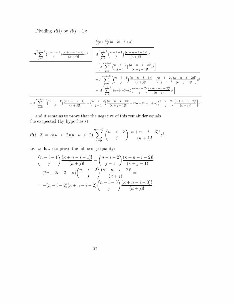
Dividing R(i) by R(i+ 1):

A

Bz +

A

B(2n − 2i − 3 + κ)

B

n−i−2X

j=0

“n − i − 2

j

” (κ + n − i − 2)!

(κ + j)!zj A

n−i−1X

j=0

“n − i − 1

j

” (κ + n − i − 1)!

(κ + j)!zj

−

»

A

n−i−1X

j=1

“n − i − 2

j − 1

” (κ + n − i − 2)!

(κ + j − 1)!zj

–

= A

n−i−2X

j=0

»

“n − i − 1

j

” (κ + n − i − 1)!

(κ + j)!−

“n − i − 2

j − 1

” (κ + n − i − 2)!

(κ + j − 1)!

–

zj

−

»

A

n−i−2X

j=0

(2n−2i−3+κ)“n − i − 2

j

” (κ + n − i − 2)!

(κ + j)!zj

–

= A

n−i−3X

j=0

»

“n − i − 1

j

” (κ + n − i − 1)!

(κ + j)!−

“n − i − 2

j − 1

” (κ + n − i − 2)!

(κ + j − 1)!− (2n − 2i − 3 + κ)

“n − i − 2

j

” (κ + n − i − 2)!

(κ + j)!

–

zj

and it remains to prove that the negative of this remainder equalsthe excpected (by hypothesis)

R(i+2) = A(n−i−2)(κ+n−i−2)

n−i−3∑

j=0

(n− i− 3

j

)(κ + n− i− 3)!

(κ + j)!zj ,

i.e. we have to prove the following equality:(n− i− 1

j

)(κ + n− i− 1)!

(κ + j)!−

(n− i− 2

j − 1

)(κ+ n− i− 2)!

(κ + j − 1)!

− (2n− 2i− 3 + κ)

(n− i− 2

j

)(κ+ n− i− 2)!

(κ+ j)!=

= −(n− i− 2)(κ+ n− i− 2)

(n− i− 3

j

)(κ+ n− i− 3)!

(κ+ j)!.

27

But“n − i − 1

j

” (κ + n − i − 1)!

(κ + j)!−

“n − i − 2

j − 1

” (κ + n − i − 2)!

(κ + j − 1)!− (2n − 2i − 3 + κ)

“n − i − 2

j

” (κ + n − i − 2)!

(κ + j)!

=(n − i − 1)!

j!(n − i − j − 1)!

(κ + n − i − 1)!

(κ + j)!−

(n − i − 2)!

(j − 1)!(n − i − j − 1)!

(κ + n − i − 2)!

(κ + j − 1)!

− (2n − 2i − 3 + κ)(n − i − 2)!

j!(n − i − j − 2)!

(κ + n − i − 2)!

(κ + j)!

=(n − i − 3)!(n − i − 2)(n − i − 1)(κ + n − i − 3)!(κ + n − i − 2)(κ + n − i − 1)

j!(n − i − j − 1)(n − i − j − 2)(n − i − j − 3)!(κ + j)!

−(n − i − 3)!(n − i − 2)j(κ + n − i − 3)!(κ + n − i − 2)(c + j)

j!(n − i − j − 3)!(n − i − j − 2)(n − i − j − 1)(κ + j)!

− (2n − 2i − 3 + κ)(n − i − 3)!(n − i − 2)(κ + n − i − 3)!(κ + n − i − 2)

j!(n − i − j − 3)!(n − i − j − 2)(κ + j)!

= (n − i − 2)(κ + n − i − 2)(n − i − 3)!

j!(n − i − j − 3)!

(κ + n − i − 3)!

(κ + j)!

·

»

(n − i − 1)(κ + n − i − 1) − j(κ + j) − (2n − 2i − 3 + κ)(n − i − j − 1)

(n − i − j − 1)(n − i − j − 2)

–

= (n − i − 2)(κ + n − i − 2)(n − i − 3)!

j!(n − i − j − 3)!

(κ + n − i − 3)!

(κ + j)!(−1)

= −(n − i − 2)(κ + n − i − 2)“n − i − 3

j

” (κ + n − i − 3)!

(κ + j)!.

References

[1] Robert B. Ash: Complex variables, Academic Press, INC. 1971.

[2] E.J. Barbeau: Polynomials, Springer-Vlg, cop. 1989.

[3] Tanja Bergkvist, Hans Rullgard: On polynomial eigenfunctionsfor a class of differential operators, Mathematical Research Let-ters 9, p. 153-171 (2002).

[4] Tanja Bergkvist, Hans Rullgard, Boris Shapiro: On Bochner-Krall orthogonal polynomial systems, to appear in MathematicaScandinavia in the spring of 2003.

[5] P. Deift, X. Zhou: A steepest descent method for oscillatoryRiemann-Hilbert problems, asymptotics for the mKDV equa-tion, Ann. Math. 137, (1993), p.295-368.

[6] H. Dette, W. Studden: Some new asymptotic properties for thezeros of Jacobi, Laguerre and Hermite polynomials, Construc-tive Approx. 11 (1995).

28

[7] K. Driver, P. Duren: Zeros of the hypergeometric polynomialsF (−n, b; 2b; z), Indag. Math. 11 (2000), p. 43-51.

[8] K. Driver, P. Duren: Trajectories of the zeros of hypergeometricpolynomials F (−n, b; 2b; z) for b < −1

2, Constr. Approx. 17

(2001), p.169-179.

[9] T. Dunster: Uniform asymptotic expansions for the reversegeneralized Bessel polynomials and related functions, SIAM J.Math. Anal. 32 (2001), p. 987-1013.

[10] Erdlyi, Magnus, Oberhettinger, Tricomi: Higher Transcenden-tal Functions, California Institute of Thechnology, McGraw-HillBook Company, INC. 1953.

[11] Jutta Faldey, Wolfgang Gawronski: On the limit distributionof the zeros of Jonquire polynomials and generalized classicalorthogonal polynomials, Journal of Approximation Theory 81,231-249 (1995).

[12] W. Gawronski: On the asymptotic distribution of the zeros ofHermite, Laguerre and Jonquire polynomials, J. Approx. The-ory 50 (1987), p.214-231.

[13] W. Gawronski: Strong asymptotics and the asymptotic zero

distribution of Laguerre polynomials L(an+α)n and Hermite poly-

nomials H(an+α)n , Analysis 13 (1993), p.29-67.

[14] A.B.J. Kuijlaars, K.T-R McLaughlin: Asymptotic zero be-haviour of Laguerre polynomials with negative parameter, toappear.

[15] A.B.J. Kuijlaars, K.T-R McLaughlin: Riemann-Hilbert anal-ysis for Laguerre polynomials with large negative parameter,Comput. Methods Func. Theory, to appear. (preprint math.CA/0204248)

[16] A.B.J. Kuijlaars, K.T-R McLaughlin, W. Van Assche, M.Vanlessen: The Riemann-Hilbert approach to strong asymp-totics for orthogonal polynomials on [−1, 1], manuscript, 2001.(preprint math. CA/0111252).

29

[17] A.B.J. Kuijlaars, W Van Assche: The asymptotic zero distri-bution of orthogonal polynomials with varying recurrence coef-ficients, J. Approx. Theory 99 (1999), p. 167-197.

[18] W. Lawton: On the zeros of certain polynomials related toJacobi and Laguerre polynomials, Bulletin of The AmericanMathematical Society, series 2, 38, 1932.

[19] Lebedev:Special functions and their applications, Prentice-Hall,INC.,1965.

[20] Gisli Masson, Boris Shapiro: A note on polynomial eigenfunc-tions of a hypergeometric type operator, Experimental Mathe-matics 10, no. 4, p. 609-618.

[21] E.B. Saff, R. Varga: On the zeros and poles of Pad approxi-mants to ez, Numer. Math. 30 (1978), p. 241-266.

[22] Slater: Confluent hypergeometric functions, Cambridge Univer-sity Press, 1960.

[23] Szeg: Orthogonal polynomials, vol. 23, AMS Colloqium Publ,1959.

[24] Watson: Thoery of Bessel Functions, Cambridge UniversityPress, 1944.

[25] Watson, Whittaker: Modern Analysis, Cambridge UniversityPress, 1940.

[26] R. Wong, J.M. Zhang: Asymptotic expansions of the gener-alized Bessel polynomials, J. Comput. Appl. Math. 85 (1997),p.87-112.

30

PAPER IV

On Asymptotics of PolynomialEigenfunctions for Degenerate

Exactly-Solvable Differential Operators

Tanja BergkvistAccepted for publication in

Journal of Approximation Theory.

Abstract

In this paper we study roots of eigenpolynomials of de-generate exactly-solvable differential operators, i.e. T =∑k

j=1QjDj with polynomial coefficients Qj in one complex

variable satisfying the condition degQj ≤ j with equalityfor at least one j, and in particular degQk < k. We showthat the root with the largest modulus of the nth degreeunique and monic eigenpolynomial pn of T tends to in-finity when n → ∞, as opposed to the non-degeneratecase (degQk = k), which we have treated previously in[2]. Our main result in this paper is an explicit conjectureand partial results on the growth of the largest modulusof the roots of pn. Based on this conjecture we deduce thealgebraic equation satisfied by the Cauchy transform ofthe asymptotic root measure of the appropriately scaledeigenpolynomials, for which the union of all roots is con-jecturally contained in a compact set.

1 Introduction

In this paper we study asymptotic properties of roots in certainfamilies of eigenpolynomials. Namely, consider a linear differentialoperator

T =k∑

j=1

QjDj ,

where D = d/dz and the Qj are complex polynomials in a sin-gle variable z satisfying the condition degQj ≤ j for all j, anddegQk < k for the leading term. Such operators will be referredto as degenerate exactly-solvable operators, see Definition 1 below.

1

In this paper we study polynomial eigenfunctions of such operators,that is polynomials satisfying

T (pn) = λnpn (1)

for some value of the spectral parameter λn, where n is a positiveinteger and deg pn = n.

The basic motivation for this study comes from two sources: 1)a classical question going back to S. Bochner, and 2) the generalizedBochner problem, which we describe below.

1) In 1929 Bochner asked about the classification of differentialequations (1) having an infinite sequence of orthogonal polynomialsolutions, see [15]. Such a system of polynomials pn∞n=0 which areboth eigenpolynomials of some finite order differential operator andorthogonal with respect to some suitable inner product, are referredto as Bochner-Krall orthogonal polynomial systems (BKS), and thecorresponding operators are called Bochner-Krall operators. It is anopen problem to classify all BKS - a complete classification is onlyknown for Bochner-Krall operators of order k ≤ 4, and the corre-sponding BKS are various classical systems such as the Jacobi type,the Laguerre type, the Legendre type and the Bessel and Hermitepolynomials, see [7].

2) The problem of a general classisfication of linear differential op-erators for which the eigenvalue problem (1) has a certain numberof eigenfunctions in the form of a finite-order polynomial in somevariables, is referred to as the generalized Bochner problem, see [19]and [20]. In the former paper a classification of operators possessinginfinitely many finite-dimensional subspaces with a basis in poly-nomials is presented, and in the latter paper a general method hasbeen formulated for generating eigenvalue problems for linear differ-ential operators in one and several variables possessing polynomialsolutions.

Notice that for the operators considered here the sequence ofeigenpolynomials is in general not an orthogonal system and it cantherefore not be studied by means of the extensive theory known forsuch systems.

2

Definition 1. We call a linear differential operator T of the kthorder exactly-solvable if it preserves the infinite flag P0 ⊂ P1 ⊂ P2 ⊂· · · ⊂ Pn ⊂ · · · , where Pn is the linear space of all polynomials ofdegree less than or equal to n.1 Or, equivalently, the problem (1)has an infinite sequence of polynomial eigenfunctions if and only ifthe operator T is exactly-solvable, see [21].

Notice that any exactly-solvable operator is of the form T =∑kj=1QjD

j. They split into two major classes: non-degenerate anddegenerate, where in the former case degQk = k, and in the lattercase degQk < k for the leading term. The major difference betweenthese two classes is that in the non-degenerate case the union of allroots of all eigenpolynomials of T is contained in a compact set (see[2]), contrary to the degenerate case, which we prove in this paper.

The importance of studying eigenpolynomials of exactly-solvableoperators is among other things motivated by numerous examplescoming from classical orthogonal polynomials. Our study can beconsidered as a natural generalization of the behaviour of the max-imal root for classical orthogonal polynomial families such as theLaguerre and Hermite polynomials, which appear as solutions tothe eigenvalueproblem (1) for certain choices on the polynomial co-efficients Qj for a second-order degenerate exactly-solvable opera-tor; the Laguerre polynomials appear as solutions to the differentialequation zy′′(z) + (1 − z)y′(z) + ny(z) = 0, and the Hermite poly-nomials are solutions to the differential equation y′′(z) − 2zy′(z) +2ny(z) = 0 where n is a nonnegative integer. Recent studies andinteresting results on the asymptotic zero behaviour for these poly-nomials and the corresponding generalized polynomials can be foundin e.g [6], [9],[13], [17], [18], [11], [12] and references therein. In [11]one can find bounds on the spacing of zeros of certain functionsbelonging to the Laguerre-Polya class satisfying a second order dif-ferential equation, and as a corollary new sharp inequalities on theextreme zeros of the Hermite, Laguerre and Jacobi polynomials areestablished.

1Correspondingly, a linear differential operator of the kth orderis called quasi-exactly-solvable if it preserves the space Pn for somefixed n.

3

Let us briefly recall our previous results. In [2] we treated theasymptotic zero distribution for polynomial families appearing assolutions to (1) where T is an arbitrary non-degenerate exactly-solvable operator. This seems to be a natural generalization tohigher orders of the Gauss hypergeometric equation. As a specialcase, the Jacobi polynomials appear as solutions to (z2 − 1)y′′(z) +(az + b)y′(z) + cy(z) = 0, where a, b and c are constants satisfyinga > b, a+b > 0 and c = n(1−a−n) for some nonnegative integer n.It is a classical fact that the zeros of the Jacobi polynomials lie in theinterval [−1, 1] and that their density in this interval is proportional

to 1/√

1 − |z|2 when the degree n tends to infinity, which followsfrom the general theory of orthogonal polynomial systems. However,for higher-order operators of this kind, the sequence of eigenpolyno-mials is in general not an orthogonal system. In [2] we proved thatwhen n → ∞, the roots of the nth degree eigenpolynomial pn for anon-degenerate exactly-solvable operator are distributed accordingto a certain probability measure which has compact support andwhich depends only on the leading polynomial Qk. Namely,

Theorem A. Let Qk be a monic polynomial of degree k. Thenthere exists a unique probability measure µQk

with compact support

whose Cauchy transform C(z) =∫ dµQk

(ζ)

z−ζsatisfies C(z)k = 1/Qk(z)

for almost all z ∈ C.

Theorem B. Let Qk and µQkbe as in Theorem A. Then supp

µQkis the union of finitely many smooth curve segments, and each

of these curves is mapped to a straight line by the locally definedmapping Ψ(z) =

∫Qk(z)

−1/kdz. Moreover, supp µQkcontains all

the zeros of Qk, is contained in the convex hull of the zeros of Qk

and is connected and has connected complement.

If pn is a polynomial of degree n we construct the probabilitymeasure (root measure) µn by placing the point mass of size 1

nat

each zero of pn. The following is our main result from [2]:

Theorem C. Let pn be the monic degree n eigenpolynomial of anon-degenerate exactly-solvable operator, and let µn be the root mea-sure of pn. Then µn converges weakly to µQk

when n→ ∞.

4

To illustrate, we show the zeros of some polynomial eigenfunc-tions for the non-degenerate exactly-solvable operator T = Q5D

5,where Q5 = (z − 2 + 2i)(z + 1 − 2i)(z + 3 + i)(z + 2i)(z − 2i− 2).In the pictures below large dots represent the zeros of Q5 and smalldots represent the zeros of the eigenpolynomials p50, p75 and p100

respectively.

-3 -2 -1 0 1 2-2

-1

0

1

2

-3 -2 -1 0 1 2-2

-1

0

1

2

-3 -2 -1 0 1 2-2

-1

0

1

2

n=50 n=75 n=100.

As a consequence of the above results we were able to prove aspecial case of a general conjecture describing the leading terms ofall Bochner-Krall operators, see [3].

In the present paper we partially extend the above results tothe case of degenerate exactly-solvable operators. Numerical evi-dence shows that the roots of the nth degree eigenpolynomial aredistributed on a tree in this case too, but that the limiting rootmeasure is compactly supported only after an appropraite scaling ofthe roots. In what follows we will wlog assume that pn is monic.

We start with the following preliminary result:

Lemma 1. Let T =∑k

j=1QjDj be a degenerate exactly-solvable

operator of order k. Then, for all sufficiently large integers n, thereexists a unique constant λn and a unique monic polynomial pn ofdegree n which satisfy T (pn) = λnpn. If degQj = j for precisely onevalue j < k, then there exists a unique constant λn and a uniquemonic polynomial pn of degree n which satisfy T (pn) = λnpn forevery integer n = 1, 2, . . ..

5

In what follows we denote by rn the largest modulus of all roots ofthe unique and monic nth degree eigenpolynomial pn of T , i.e.

rn = max|z| : pn(z) = 0.

These are our main results:

Theorem 1.2 Let T be a degenerate exactly-solvable operator oforder k. Then rn → ∞ when n→ ∞.

Next we establish a lower bound for rn when n→ ∞.

Theorem 2. Let T =∑k

j=1QjDj =

∑kj=1

(∑deg Qj

i=0 αj,izi)Dj be a

degenerate exactly-solvable operator of order k. Then for any γ < bwe have

limn→∞

rn

nγ= ∞,

where

b :=+

minj∈[1,k−1]

(k − j

k − j + degQj − degQk

),

and where the notation min+ means that the minimum is taken onlyover positive terms (k − j + degQj − degQk).

Corollary 1. Let T =∑k

j=1QjDj be a degenerate exactly-solvable

operator of order k such that degQj ≤ j0 for all j > j0, and in par-ticular degQk = j0, where j0 is the largest j such that degQj = j.Then limn→∞

rn

nγ = ∞ for any γ < 1.

Corollary 2. Let T =∑k

j=1QjDj be a degenerate exactly-solvable

operator of order k such that degQj = 0 for all j > j0, where j0 isthe largest j for which degQj = j. Then limn→∞

rn

nγ = ∞ for any

γ < k−j0k

.

In fact our extensive numerical experiments and natural heuristicarguments (see Section 3) support the following conjecture:

2This theorem is joint work with H. Rullgard.

6

Main Conjecture. Let T =∑k

j=1QjDj be a degenerate exactly-

solvable operator of order k and denote by j0 the largest j for whichdegQj = j. Then

limn→∞

rn

nd= cT ,

where cT > 0 is a positive constant and

d := maxj∈[j0+1,k]

(j − j0

j − degQj

).

Remark. Note that Main Conjecture implies Theorem 2 sinceb ≤ d.

The next two theorems support the above conjecture:

Theorem 3. Let T be a degenerate exactly-solvable operator of or-der k consisting of precisely two terms: T = Qj0D

j0 +QkDk. Then

there exists a positive constant c such that

limn→∞

infrn

nd≥ c

where d := maxj∈[j0+1,k]

(j−j0

j−deg Qj

)= k−j0

k−deg Qk.

This result can be generalized to operators consisting of any numberof terms, but with certain conditions on the degree of the polyno-mial coefficients Qj when j > j0, where j0 is the largest j for whichdegQj = j. Namely,

Theorem 4. Let T be a degenerate exactly-solvable operator oforder k. Denote by j0 the largest j such that degQj = j and let(j − degQj) ≥ (k − degQk) for every j > j0. Then there exists apositive constant c > 0 such that

limn→∞

infrn

nd≥ c

where d := maxj∈[j0+1,k]

(j−j0

j−deg Qj

)= k−j0

k−deg Qk.

Computer experiments indicate that roots of eigenpolynomialsscaled according to the Main Conjecture fill certain interesting curves

7

in C. To illustrate this phenomenon let us present some typical pic-tures. Below pn denotes the nth degree unique and monic eigenpoly-nomial of the given operator, and qn(z) = pn(ndz) denotes the cor-responding appropriately scaled polynomial, where d is as in MainConjecture, and for which the union of all roots is (conjecturally)contained in a compact set.

Fig.1: Fig.2: Fig.3:

-2 -1.5 -1 -0.5 0-1.5

-1

-0.5

0

0.5

1

1.5

-1 -0.5 0 0.5 1

-1

-0.5

0

0.5

1

-0.4 -0.2 0 0.2 0.4

-1

-0.5

0

0.5

1

roots of roots of roots ofq100(z) = p100(100z) q100(z) = p100(100z) q100(z) = p100(100z)

Fig.1: T1 = zD + zD2 + zD3 + zD4 + zD5.Fig.2: T2 = z2D2 +D7.Fig.3: T3 = z3D3 + z2D4 + zD5.

In Section 3 we will derive the (conjectural) algebraic equationsatisfied by the Cauchy transform C(z) of the asymptotic root mea-sure of the scaled eigenpolynomial qn for an arbitrary degenerateexactly-solvable operator. From this equation one can obtain de-tailed information about the above curves and also conclude whichterms of the operator that are relevant for the asymptotic zero dis-tribution of its eigenpolynomials.3 Namely, with d and j0 as in MainConjecture and assuming Qj0 is monic, we have

zj0Cj0(z) +∑

j∈A

αj,deg Qjzdeg QjCj(z) = 1,

where A = j : (j−j0)/(j−degQj) = d and αj,deg Qjis the leading

coefficient of Qj . For details see Section 3.

3As was mentioned earlier, in the non-degenerate case which wehave treated previously, the asymptotic zero distribution of theeigenpolynomials depends only on the leading coefficient Qk. Forthe operators considered here however, the situation is more com-plicated.

8

Numerical evidence clearly illustrates that distinct operators whosescaled eigenpolynomials satisfy the same Cauchy transform equationwhen n→ ∞, will yield identical asymptotic zero distributions. Be-low we show one such example. For further details see Section 4.3.

-1 -0.5 0 0.5

-1

-0.5

0

0.5

1

-1 -0.5 0 0.5

-1

-0.5

0

0.5

1

T4, roots of T4, roots ofq100(z) = p100(1002/3z) q100(z) = p100(1002/3z)

where T4 = z3D3 + z2D5 and T4 = z2D2 + z3D3 + zD4 + z2D5 +D6.

Let us finally mention some possible applications of our resultsand directions for further research. As was mentioned earlier, oper-ators of the type we consider occur in the theory of Bochner-Krallorthogonal systems. A great deal is known about the asymptoticzero distribution of orthogonal polynomials. By comparing suchknown results with results on the asymptotic zero distribution ofthe eigenpolynomials considered here, we believe it will be possibleto gain new insight into the nature of BKS.

This paper is structured as follows. In Section 2 we give theproofs of the lemma, the theorems and the corollaries stated in thissection. In Section 3 we explain how we arrived at Main Conjectureand how we obtain as its corollary the algebraic Cauchy transformequation. In Section 4 we display numerical evidence supportingMain Conjecture and its corollary. In Section 5 (Appendix) wegive the detailed calculations which led to the corollary of MainConjecture, and we also prove that for a class of operators of thetype we consider, the conjectured upper bound for rn implies theconjectured lower bound. Finally, in Section 6, we discuss someopen problems and directions for further research.

9

Acknowledgements. I am sincerely greatful to my PhD advi-sor Professor B. Shapiro for introducing me to this very fascinatingproblem and for his constant support during my work. I would alsolike to thank Professor J-E. Bjork for stimulating discussions on thetopic. I am also indepted to anonymous referees for their interest-ing suggestions which contributed to the improvement of this paper.My research was supported by Stockholm University.

2 Proofs

Proof of Lemma 1. In [2] we proved that for any exactly-solvableoperator T , the eigenvalue problem T (pn) = λnpn can be writ-ten as a linear system MX = Y , where X is the coefficient vec-tor of the monic nth degree eigenpolynomial pn with componentsan,0, an,1, an,2, . . . , an,n−1, and Y is a vector and M is an uppertriangular n × n matrix, both with entries expressible in the co-

efficients of T . With T =∑k

j=1QjDj, Qj =

∑deg Qj

i=0 αj,izi, and

pn(z) =∑n

i=0 an,izi, the eigenvalue λn is given by

λn =k∑

j=1

αj,jn!

(n− j)!,

and the diagonal elements of the matrix M are given by

Mi+1,i+1 =∑

1≤j≤min(i,k)

αj,ji!

(i− j)!−λn =

k∑

j=1

αj,j

[i!

(i− j)!− n!

(n− j)!

]

for i = 0, 1, . . . , n− 1. The last equality follows since i!/(i− j)! = 0for i < j ≤ k by definition (see Lemma 2 in [2]). In order to provethat pn is unique we only need to check that the determinant of Mis nonzero, which implies that M is invertible, whence the systemMX = Y has a unique solution. Notice that M is upper trian-gular and thus its determinant equals the product of its diagonalelements. We therefore prove that every diagonal element Mi+1,i+1

(i ∈ [0, n − 1]) is nonzero for all sufficiently large integers n for anarbitrary T as above, as well as for every n if degQj = j for exactlyone j.

10

From the expression

−Mi+1,i+1 =k∑

j=1

αj,j

[n!

(n− j)!− i!

(i− j)!

]

it is clear that Mi+1,i+1 6= 0 for every i ∈ [0, n − 1] and every n ifαj,j 6= 0 for exactly one j, that is if degQj = j for precisely one j,and thus we have proved the second part of Lemma 1.

Now assume that degQj = j for more than one j and denote byj0 the largest such j. Then αj0,j0 6= 0 and we have

− Mi+1,i+1 =

j0∑

j=1

αj,j

[n!

(n− j)!− i!

(i− j)!

]

=n!

(n− j0)!

[αj0,j0

(1 − i!/(i− j0)!

n!/(n− j0)!

)+

∑

1≤j<j0

αj,j(n− j0)!

(n− j)!

−∑

1≤j<j0

(n− j0)!i!

n!(i− j)!

].

The last two sums in the brackets on the right-hand side of the aboveequality tend to zero when n→ ∞, since j0 > j and i ≤ n−1. Thusfor all sufficiently large n we get

−Mi+1,i+1 =n!

(n− j0)!

[αj0,j0

(1 − i!/(i− j0)!

n!/(n− j0)!

)]6= 0

for every i ∈ [0, n− 1], and we have proved the first part of Lemma1.

To prove Theorem 1 we need the following. If pn is a polynomialof degree n we construct the probability measure µn by placing apoint mass of size 1

nat each zero of pn. We call µn the root measure

of pn. By definition, for any polynomial pn of degree n, the Cauchy

transform Cn,j of the root measure µ(j)n for the jth derivative p

(j)n is

defined by

Cn,j(z) :=p

(j+1)n (z)

(n− j)p(j)n (z)

=

∫dµ

(j)n (ζ)

z − ζ,

11

for j = 0, 1, . . . , n − 1, and it is well-known that the measure µ(j)n

can be reconstructed from Cn,j by the formula µ(j)n = 1

π· ∂Cn,j

∂zwhere

∂/∂z = 12(∂/∂x + i∂/∂y).

Proof of Theorem 1. Let T =∑k

j=1QjDj and denote by j0

the largest j for which degQj = j. Note that since T is degeneratewe have j0 < k. Thus, using the above notation, we have

p(j)n (z)

pn(z)= Cn,0(z)Cn,1(z) · · ·Cn,j−1(z) · n(n− 1) · · · (n− j + 1)

=n!

(n− j)!

j−1∏

m=0

Cn,m(z).

With the notationQj(z) =∑deg Qj

i=0 αj,izi we have λn =

∑j0j=1 αj,j

n!(n−j)!

.

Now dividing the equation T (pn) = λnpn by pn we obtain

Qk(z)p

(k)n (z)

pn(z)+Qk−1(z)

p(k−1)n (z)

pn(z)+ . . .+Q1(z)

p′n(z)

pn(z)=

j0∑

j=1

αj,jn!

(n− j)!

⇔

Qk(z)n!

(n− k)!

k−1∏

m=0

Cn,m(z) +Qk−1(z)n!

(n− k + 1)!

k−2∏

m=0

Cn,m(z) + . . .

. . .+Q1(z)n!

(n− 1)!Cn,0(z) =

j0∑

j=1

αj,jn!

(n− j)!. (2)

Dividing both sides of this equation by n!(n−k)!

we get

Qk(z)

k−1∏

m=0

Cn,m(z)

[1 +

(n− k)!

(n− k + 1)!

1

Cn,k−1(z)

Qk−1(z)

Qk(z)+

(n− k)!

(n− k + 2)!

1

Cn,k−1(z)Cn,k−2(z)

Qk−2(z)

Qk(z)+ . . .

. . .+(n− k)!

(n− 1)!

1∏k−1

m=1Cn,m(z)

Q1(z)

Qk(z)

]=

j0∑

j=1

αj,j(n− k)!

(n− j)!. (3)

Now assume that all zeros of all pn are uniformly bounded. Thenwe can take a subsequence pni

such that all the corresponding

12

root measures µniare weakly convergent to a compactly supported

probability measure. Then all Cauchy transforms Cni,m will be uni-formly convergent to a non-vanishing function outside some largedisc, which in particular contains all the roots ofQk(z). Since j0 < k,the right-hand side of (3) tends to zero when n→ ∞. On the otherhand, in the left-hand side of (3), all terms in the bracket except forthe constant term 1 tend to zero when n → ∞, and thus the limitof the left-hand side equals limn→∞Qk(z)

∏k−1m=0 Cn,m(z) = K 6= 0,

and we obtain a contradiction when n→ ∞.

In order to prove Theorem 2 we need the following two lemmas,where Lemma 2 is used to prove Lemma 3.

Lemma 2. Let zn be a root of pn with the largest modulus rn.Then, for any complex number z0 such that |z0| = r0 ≥ rn, we have|Cn,j(z0)| ≥ 1

2r0for all j ≥ 0.

Proof. Recall that Cn,j(z) :=∫ dµ

(j)n (ζ)z−ζ

= p(j+1)n (z)

(n−j)p(j)n (z)

. With ζ being

some root of p(j)n (z) we have |ζ | ≤ |z0| by Gauss-Lucas theorem.

Thus 1z0−ζ

= 1z0

· 11−ζ/z0

= 1z0

· 11−θ

where |θ| = |ζ/z0| ≤ 1. With

w = 11−θ

we obtain

|w − 1| =|θ|

|1 − θ| = |θ||w| ≤ |w| ⇔ |w − 1| ≤ |w| ⇒ Re(w) ≥ 1/2,

and thus

|Cn,j(z0)| =

∣∣∣∣∫dµ

(j)n (ζ)

z0 − ζ

∣∣∣∣ =1

r0

∣∣∣∣∫dµ

(j)n (ζ)

1 − θ

∣∣∣∣ =1

r0

∣∣∣∣∫wdµ(j)

n (ζ)

∣∣∣∣

≥ 1

r0

∣∣∣∣∫Re(w)dµ(j)

n (ζ)

∣∣∣∣ ≥1

2r0

∫dµ(j)

n (ζ) =1

2r0.

Lemma 3. Let T =∑k

j=1QjDj =

∑kj=1

( ∑deg Qj

i=0 αj,izi)Dj be a

degenerate exactly-solvable operator of order k. Wlog we assumethat Qk is monic, i.e. αk,deg Qk

= 1. Let zn be a root of pn with thelargest modulus rn. Then the following inequality holds:

13

1 ≤k−1∑

j=1

deg Qj∑

i=0

|αj,i|2k−j rk−j−degQk+in

(n− k + 1)k−j+

∑

0≤i<deg Qk

|αk,i|rdeg Qk−in

. (4)

Proof. From Cn,j(z) = p(j+1)n (z)

(n−j)p(j)(z)we get

p(j)(z) =p

(k)n (z)

(n− k + 1)(n− k + 2) · · · (n− j)∏k−1

m=j Cn,m(z)(5)

for all j < k. Inserting zn in the eigenvalue equation Tpn(z) =λnpn(z) we obtain

k−1∑

j=1

( deg Qj∑

i=0

αj,izin

)p(j)

n (zn) +

( deg Qk∑

i=0

αk,izin

)p(k)

n (zn) = λnpn(zn) = 0,

and after division by zdeg Qkn p

(k)n (zn) we obtain

k−1∑

j=1

( deg Qj∑

i=0

αj,i1

zdeg Qk−in

)p

(j)n (zn)

p(k)n (zn)

+∑

0≤i<deg Qk

αk,i1

zdeg Qk−in

+ 1 = 0.

Thus, applying (5) and Lemma 2, we obtain

1 =

∣∣∣∣k−1∑

j=1

( deg Qj∑

i=0

αj,i1

zdeg Qk−in

)p

(j)n (zn)

p(k)n (zn)

+∑

0≤i<deg Qk

αk,i1

zdeg Qk−in

∣∣∣∣

≤k−1∑

j=1

∣∣∣∣deg Qj∑

i=0

αj,i1

zdeg Qk−in

∣∣∣∣|p(j)

n (zn)||p(k)

n (zn)|+

∑

0≤i<deg Qk

|αk,i|rdeg Qk−in

≤k−1∑

j=1

deg Qj∑

i=0

|αj,i|rdeg Qk−in

1

(n− k + 1) · · · (n− j)∏k−1

m=j |Cn,m(zn)|

+∑

0≤i<deg Qk

|αk,i|rdeg Qk−in

≤k−1∑

j=1

deg Qj∑

i=0

|αj,i|rdeg Qk−in

(2rn)k−j

(n− k + 1)k−j+

∑

0≤i<deg Qk

|αk,i|rdeg Qk−in

=k−1∑

j=1

deg Qj∑

i=0

|αj,i|2k−j rk−j−degQk+in

(n− k + 1)k−j+

∑

0≤i<deg Qk

|αk,i|rdeg Qk−in

.

14

The proof of Theorem 2 follows from Theorem 1 and Lemma 3.

Proof of Theorem 2. Applying Theorem 1, we see that the lastsum on the right-hand side of inequality (4) in Lemma 3 tends to zerowhen n→ ∞. Now consider the double sum on the right-hand sideof (4). If, for given i and j, the exponent (k− j−degQk + i) of rn isnegative or zero, the corresponding term tends to zero when n→ ∞by Theorem 1. We now consider the remaining terms in the doublesum, namely those for which the exponent (k−j−degQk+i) of rn ispositive. If rn ≤ c0(n−k+1)γ where c0 > 0 and γ < k−j

k−j+i−deg Qkfor

given j ∈ [1, k− 1] and given i ∈ [0, degQj ], then the correspondingterm

rk−j+i−deg Qkn

(n− k + 1)k−j=

(rn

(n− k + 1)k−j

k−j+i−deg Qk

)k−j+i−deg Qk

in the double sum tends to zero when n → ∞. Thus assume thatrn ≤ c0(n− k+ 1)γ where c0 is a positive constant and γ < b where

b =+

minj∈[1,k−1]

i∈[0,j]

k − j

k − j + i− degQk=

+

minj∈[1,k−1]

k − j

k − j + degQj − degQk,

and where the notation min+ means that we only take the minimumover positive terms (k−j+i−degQk) and (k−j+degQj−degQk).

4

Then every term in the double sum tends to zero when n→ ∞, andwe obtain a contradiction to (4) when n → ∞. Thus for all suf-ficiently large integers n we must have rn > c0(n − k + 1)γ for allγ < b, and hence lim infn→∞

rn

nγ > c0 for any γ < b. But for any

such γ we can form γ′

= γ+b2

for which γ′

< b and γ < γ′

, and thuslimn→∞

rn

nγ = ∞ for all γ < b.

4On the left-hand side in the expression for b above we take theminimum over i ∈ [0, degQj ], so we can put i = degQj in this

expression. Thus with b = min+j∈[1,k−1]

k−jk−j+deg Qj−deg Qk

we get that

γ < k−jk−j+i−deg Qk

for every j ∈ [1, k − 1] and every i ∈ [0, degQj ].

Then if rn ≤ c0(n − k + 1)γ and γ < b, every term with positiveexponent (k − j + i− degQk) will tend to zero when n→ ∞.

15

Proof of Corollary 1. For this class of operators we have

b :=+

minj∈[1,k−1]

k − j

k − j + degQj − degQk

=+

minj∈[1,k−1]

k − j

k − j + degQj − j0=k − j0k − j0

= 1,

and the proof is complete applying Theorem 2.

Proof of Corollary 2. For this class of operators we have

b :=+

minj∈[1,k−1]

(k − j

k − j + degQj − degQk

)

=+

minj∈[1,k−1]

(k − j

k − j + degQj

)= min

j∈[1,j0]

k − j

k=k − j0k

where the third equality follows from choosing any j for whichdegQj = j, and the minimum is then attained for j = j0 (notethat for j > j0 we get (k − j)/(k − j + degQj) = 1 > (k − j0)/k),and the proof is complete applying Theorem 2.

Remark. Note that for the class of operators considered in Corol-lary 1 the Main Conjecture claims that limn→∞

rn

n= cT for some

cT > 0, since d := maxj∈[j0+1,k]

(j−j0

j−deg Qj

)= k−j0

k−j0= 1 (the maxi-

mum is attained by choosing any j > j0 such that degQj = j0, e.g.j = k), and for the class of operators considered in Corollary 2 theMain Conjecture claims that limn→∞

rn

n(k−j0)/k = cT for some cT > 0,since

d := maxj∈[j0+1,k]

(j − j0

j − degQj

)= max

j∈[j0+1,k]

(j − j0j

)=k − j0k

.

Remark. For a class of operators containing the operators con-sidered in Corollaries 1 and 2 we can actually prove that the con-jectured upper bound limn→∞ sup rn

nd ≤ c1 implies the conjecturedlower bound limn→∞ inf rn

nd ≥ c0 where c1 ≥ c0 > 0, see Theorem 5in Section 5.2.

Proof of Theorem 3. Clearly degQj0 = j0 since there exists

16

at least one such j < k. Set

T = Qj0Dj0 +QkD

k =

j0∑

i=0

αj0,iziDj0 +

deg Qk∑

i=0

αk,iziDk,

where αj0,j0 6= 0, and where we wlog assume that Qk is monic. Frominequality (4) in Lemma 3 we have

1 ≤j0∑

i=0

|αj0,i|2k−j0ri−deg Qk+k−j0n

(n− k + 1)k−j0+

∑

0≤i<deg Qk

|αk,i|1

rdeg Qk−in

≤j0∑

i=0

|αj0,i|2k−j0ri−deg Qk+k−j0n

(n− k + 1)k−j0+ ǫ,

where we choose n so large that ǫ < 1 (this is possible since ǫ → 0when n→ ∞ due to Theorem 1). Thus for sufficiently large n

c0 ≤j0∑

i=0

|αj0,i|2k−j0ri−deg Qk+k−j0n

(n− k + 1)k−j0

≤j0∑

i=0

|αj0,i|2k−j0rk−deg Qkn

(n− k + 1)k−j0

= Krk−deg Qkn

(n− k + 1)k−j0,

where 1− ǫ = c0 → 1 when n→ ∞, and K > 0 since αj0,j0 6= 0 (thesecond inequality follows since i ≤ j0). Thus

rn ≥( c0K

)1/(k−deg Qk)(n− k + 1)

k−j0k−deg Qk

for sufficiently large integers n, and hence there exists a positiveconstant c = (1/K)1/(k−deg Qk) such that

limn→∞

infrn

n

(k−j0

k−deg Qk

) ≥ c.

Finally, it is clear that for this two-term operator

d := maxj∈[j0+1,k]

(j − j0

j − degQj

)=

k − j0k − degQk

,

17

and we are done.

Remark. If, in Theorem 3, Qk is a monomial (i.e. Qk = zdeg Qk),then there exists a positive constant c such that rn ≥ c(n− k + 1)d

for every n, where d := maxj∈[j0+1,k]

(j−j0

j−deg Qj

)= k−j0

k−deg Qk. This is

easily seen from the calculations in the proof of Theorem 3 since∑0≤i<deg Qk

|αk,i| 1

rdeg Qk−in

on the right-hand side of (4) vanishes, and

therefore 1 ≤ K rk−deg Qkn

(n−k+1)k−j0for every n. From the second part of

Lemma 1 we know that for this class of operators there exists aunique eigenpolynomial pn for every n, and the conclusion follows.

Proof of Theorem 4. For this class of operators (j − degQj) ≥(k − degQk) for every j > j0 and thus

d := maxj∈[j0+1,k]

(j − j0

j − degQj

)=

k − j0k − degQk

.

Assuming that Qk is monic we have the inequality

1 ≤k−1∑

j=1

deg Qj∑

i=0

|αj,i|2k−j rk−j+i−deg Qkn

(n− k + 1)k−j+

∑

0≤i<deg Qk

|αk,i|rdeg Qk−in

(6)

by Lemma 3. The last sum here tends to zero when n → ∞ byTheorem 1. Considering the double sum on the right-hand side of(6) we see that for every j we have (since i ≤ degQj) that

deg Qj∑

i=0

|αj,i|2k−j rk−j+i−degQkn

(n− k + 1)k−j

=

deg Qj∑

i=0

|αj,i|2k−j rk−j+deg Qj−deg Qkn

(n− k + 1)k−jri−deg Qjn

=r

k−j+deg Qj−deg Qkn

(n− k + 1)k−j

(2k−j|αj,deg Qj

| +∑

i<deg Qj

2k−j|αj,i|ri−deg Qjn

)

= Kj,nr

k−j+deg Qj−deg Qkn

(n− k + 1)k−j, (7)

where

Kj,n = 2k−j|αj,deg Qj| +

∑

i<deg Qj

2k−j|αj,i|ri−deg Qjn ,

18

where Kj,n > 0 since αj,deg Qj6= 0. Also, Kj,n < ∞ when n →

∞ since (i − degQj) < 0 for the exponent of rn, and then usingTheorem 1 (note that Kj,n → 2k−j|αj,deg Qj

| when n → ∞). Withthe decompositionA = j : degQj = j,B = j : degQj < j and (k − j + degQj − degQk) > 0,C = j : degQj < j and (k − j + degQj − degQk) ≤ 0,and using (7) we see that inequality (6) is equivalent to:

1 ≤k−1∑

j=1

j∑

i=0

|αj,i|2k−j rk−j+i−deg Qkn

(n− k + 1)k−j+

∑

0≤i<deg Qk

|αk,i|rdeg Qk−in

=∑

j∈A

Kj,nrk−deg Qkn

(n− k + 1)k−j+

∑

j∈B

Kj,nr

k−j+deg Qj−deg Qkn

(n− k + 1)k−j

+∑

j∈C

Kj,nr

k−j+degQj−deg Qkn

(n− k + 1)k−j+

∑

0≤i<deg Qk

|αk,i|rdeg Qk−in

.

The last two sums on the right-hand side of this inequality bothtend to zero when n → ∞, the last one due to Theorem 1, and thesum over C since (j − degQj) ≥ (k − degQk) ⇔ (k − j + degQj −degQk) ≤ 0 for every j ∈ C by assumption, and then applyingTheorem 1. Therefore, when n→ ∞, we get the inequality

c0 ≤∑

j∈A

Kj,nrk−deg Qkn

(n− k + 1)k−j+

∑

j∈B

Kj,nr

k−j+deg Qj−deg Qkn

(n− k + 1)k−j(8)

where

c0 = 1 −∑

j∈C

Kj,nr

k−j+deg Qj−deg Qkn

(n− k + 1)k−j−

∑

0≤i<deg Qk

|αk,i|rdeg Qk−in

.

Note that c0 → 1 when n→ ∞.Now assume that B is empty. This corresponds to an opera-

tor such that (j − degQj) ≥ (k − degQk) for every j for whichdegQj < j. Then inequality (8) above becomes

19

c0 ≤∑

j∈A

Kj,nrk−deg Qkn

(n− k + 1)k−j

=rk−deg Qkn

(n− k + 1)k−j0

(Kj0,n +

∑

j∈A\j0

Kj,n1

(n− k + 1)j0−j

)

≤ KArk−deg Qkn

(n− k + 1)k−j0(9)

where KA is a positive constant which is finite when n → ∞, sincej0 − j > 0 for every j ∈ A\j0 (recall that j0 is the largest elementin A by definition). Thus for all sufficiently large integers n we have

rn ≥( c0KA

)1/(k−deg Qk)(n− k + 1)

k−j0k−deg Qk ,

and therefore there exists a positive constant c = (1/KA)1/(k−deg Qk)

such that

limn→∞

infrn

n

(k−j0

k−deg Qk

) ≥ c,

and we are done.

Now assume that B is nonempty. Again inequality (8) holds, i.e.

c0 ≤∑

j∈A

Kj,nrk−deg Qkn

(n− k + 1)k−j+

∑

j∈B

Kj,nr

k−j+deg Qj−deg Qkn

(n− k + 1)k−j,

where c0 → 1 when n→ ∞. From (9) we have

∑

j∈A

Kj,nrk−deg Qkn

(n− k + 1)k−j≤ KA

rk−deg Qkn

(n− k + 1)k−j0

for the sum over A for large n and thus

20

c0 ≤∑

j∈A

Kj,nrk−deg Qkn

(n− k + 1)k−j+

∑

j∈B

Kj,nr

k−j+deg Qj−deg Qkn

(n− k + 1)k−j

≤ KArk−deg Qkn

(n− k + 1)k−j0+

∑

j∈B

Kj,nr

k−j+deg Qj−deg Qkn

(n− k + 1)k−j

=rk−deg Qkn

(n− k + 1)k−j0

(KA +

∑

j∈B

Kj,nrdeg Qj−jn

(n− k + 1)j0−j

)

≤ KABrk−deg Qkn

(n− k + 1)k−j0,

where KAB is a positive and finite constant when n→ ∞ (note thatKAB → KA when n→ ∞, since (degQj − j) < 0 and j0 − j > 0 forevery j ∈ B). Thus for all sufficiently large integers n we have

rn ≥( c0KAB

)1/(k−deg Qk)(n− k + 1)

k−j0k−deg Qk ,

so there exists a positive constant c = (1/KAB)1/(k−deg Qk) such that

limn→∞

infrn

n

(k−j0

k−deg Qk

) ≥ c.

3 Main Conjecture and its Corollary

In this section we explain how we arrived at Main Conjecture (seeSection 1) and obtain as a corollary of our method the (conjectural)algebraic equation satisfied by the Cauchy transform of the asymp-totic root measure of the properly scaled eigenpolynomials.

How did we arrive at Main Conjecture?

Let T =∑k

j=1QjDj =

∑kj=1

(∑deg Qj

i=0 αj,izi)Dj be an arbitrary de-

generate exactly-solvable operator of order k and denote by j0 thelargest j for which degQj = j. Wlog we assume that Qj0 is monic,

21

i.e. αj0,j0 = 1. Consider the scaled eigenpolynomial qn(z) = pn(ndz),where pn(z) is the unique and monic nth degree eigenpolynomial ofT , and d is some real number. The goal is now to obtain a well-defined algebraic equation for the Cauchy transform of the root mea-sure µn of the scaled eigenpolynomial qn when n → ∞, and as wewill see in the process of doing this, we are forced to choose d as inMain Conjecture.5

Basic assumption. When performing our calculations we as-

sume that the root measures µ(0)n , µ

(1)n , µ

(2)n . . . , µ

(k−1)n of the scaled

eigenpolynomial qn(z) and its derivatives up to the kth order ex-ist when n → ∞ and that they are are all weakly convergent tothe same asymptotic root measure µ.6 Thus the correspondingCauchy transforms are all asymptotically identical, and we defineC(z) := limn→∞Cn,j(z) for all j ∈ [0, k − 1], where C(z) is theCauchy transform of µ and is considered for z’s away from the sup-port of µ. Computer experiments strongly indicate that this as-sumption is true - for details see Section 4.2.

From the definition of the Cauchy transform we obtain

j−1∏

i=0

Cn,i(z) =

j−1∏

i=0

q(i+1)n (z)

(n− j)q(i)n (z)

=q(1)n (z)

nqn(z)· q

(2)n (z)

(n− 1)q(1)(z)· q

(3)n (z)

(n− 2)q(2)n (z)

· · ·

· · · q(j−1)n (z)

(n− j + 2)q(j−2)n (z)

· q(j)n (z)

(n− j + 1)q(j−1)n (z)

=q(j)n (z)

n(n− 1) · · · (n− j + 1)qn(z),

5It is already well-known that for the Laguerre polynomials, whichappear as eigenpolynomials for a second order exactly-solvable op-erator, the largest root grows as n when n → ∞ and thus d = 1 inthis case, which is consistent with Main Conjecture.

6Conjecturally supp µ is a tree, see Section 6 on Open Problems.

22

and thus the basic assumption implies

Cj(z) = limn→∞

j−1∏

i=0

Cn,i(z) = limn→∞

q(j)n (z)

n(n− 1) · · · (n− j + 1)qn(z). (10)

In the above notation consider the eigenvalue equation Tpn(z) =λnpn(z), where the eigenvalue λn is given by

λn =k∑

j=1

αj,jn!

(n− j)!=

j0∑

j=1

αj,jn!

(n− j)!=

j0∑

j=1

αj,jn(n−1) · · · (n−j+1).

Clearly this sum ends at j0 since αj,j = 0 for all j > j0 by definitionof j0 as the largest j for which degQj = j. We then have

Tpn(z) = λnpn(z)

⇔k∑

j=1

( deg Qj∑

i=0

αj,izi

)p(j)

n (z) =

j0∑

j=1

αj,jn(n− 1) · · · (n− j + 1)pn(z).

Substituting z = ndz in this equation we obtain

k∑

j=1

( deg Qj∑

i=0

αj,indizi

)p(j)

n (ndz) =

j0∑

j=1

αj,jn(n−1) · · · (n−j+1)pn(ndz),

and with qn(z) = pn(ndz) we get

k∑

j=1

( deg Qj∑

i=0

αj,izi

nd(j−i)

)q(j)n (z) =

j0∑

j=1

αj,jn(n− 1) · · · (n− j +1)qn(z).

Dividing this equation by n!(n−j0)!

qn(z) = n(n−1) · · · (n−j0 +1)qn(z)we get

k∑

j=1

( deg Qj∑

i=0

αj,izi

nd(j−i)

)q(j)n (z)

n(n− 1) · · · (n− j0 + 1)qn(z)=

=

j0∑

j=1

αj,jn(n− 1) · · · (n− j + 1)

n(n− 1) · · · (n− j0 + 1). (11)

23

Consider the right-hand side of (11). Since j ≤ j0 all terms forwhich j < j0 (if not already zero, which is the case if αj,j = 0, i.e.if degQj < j) tend to zero when n→ ∞, and therefore the limit ofthe right-hand side of (11) equals

limn→∞

j0∑

j=1

αj,jn(n− 1) · · · (n− j + 1)

n(n− 1) · · · (n− j0 + 1)= αj0,j0 = 1,

since we assumed that Qj0 is monic. Now consider the jth term inthe sum on the left-hand side of (11). It equals

deg Qj∑

i=0

αj,izi

nd(j−i)· q

(j)n (z)

n(n− 1) · · · (n− j0 + 1)qn(z)=

=

deg Qj∑

i=0

αj,izi

nd(j−i)· q

(j)n (z)

n(n− 1) · · · (n− j + 1)qn(z)· n · · · (n− j + 1)

n · · · (n− j0 + 1)

=

deg Qj∑

i=0

αj,izi

nd(j−i)·

j−1∏

i=0

Cn,i(z) ·n(n− 1) · · · (n− j + 1)

n(n− 1) · · · (n− j0 + 1)

=

deg Qj∑

i=0

αj,izi

nd(j−i)+j0−j

j−1∏

i=0

Cn,i(z)n · · · (n− j + 1)

nj

nj0

n · · · (n− j0 + 1).

Taking the limit and using the basic assumption (10) we obtain

limn→∞

deg Qj∑

i=0

αj,izi

nd(j−i)· q

(j)n (z)

n(n− 1) · · · (n− j0 + 1)qn(z)

= limn→∞

deg Qj∑

i=0

αj,izi

nd(j−i)+j0−jCj(z)

for the jth term and thus, taking the limit of the left-hand side of(11) we get

limn→∞

k∑

j=1

( deg Qj∑

i=0

αj,izi

nd(j−i)

)q(j)n (z)

n(n− 1) · · · (n− j0 + 1)qn(z)

= limn→∞

k∑

j=1

( deg Qj∑

i=0

αj,izi

nd(j−i)+j0−j

)Cj(z).

24

Adding up, the following equation is satisfied by C(z) for z’s awayfrom the support of µ:

limn→∞

k∑

j=1

( deg Qj∑

i=0

αj,izi

nd(j−i)+j0−j

)Cj(z) = 1. (12)

In order to make (12) a well-defined algebraic equation, i.e. to avoidinfinities in the denominator when n→ ∞, we must impose the fol-lowing condition on the real number d in the exponent of n, namely

d(j − i) + j0 − j ≥ 0 ⇔ d ≥ j − j0j − i

for all j ∈ [1, k] and all i ∈ [0, degQj ]. Therefore we take d =max j∈[1,k]

i∈[0,deg Qj ]

(j−j0j−i

), but this maximum is clearly obtained for the

maximal value of i for any given j, so we may as well put i = degQj .Our condition then becomes d = maxj∈[1,k]

(j−j0

j−deg Qj

), and clearly

the maximum is taken only over j for which Qj(z) is not identicallyzero. Finally we observe that since T is degenerate we have j0 < kand thus we need only take this maximum over j ∈ [j0 + 1, k], sincethere always exists a positive value on d for any operator of the typewe consider. Thus our condition becomes:

d = maxj∈[j0+1,k]

(j − j0

j − degQj

).

Corollary of Main Conjecture.

In the above notation (recall that αj0,j0 = 1 by monicity of Qj0), thefollowing well-defined algebraic equation follows immediately wheninserting d as defined in Main Conjecture into equation (12) andletting n→ ∞:

Corollary. The Cauchy transform C(z) of the asymptotic root mea-sure µ of the scaled eigenpolynomial qn(z) = pn(ndz) of an exactly-solvable operator T as above with Qj0 monic satisfies the followingalgebraic equation for almost all complex z in the usual Lebesguemeasure on C:

zj0Cj0(z) +∑

j∈A

αj,deg Qjzdeg QjCj(z) = 1,

25

where A is the set consisting of all j for which the maximumd := maxj∈[j0+1,k]

(j−j0

j−deg Qj

)is attained, i.e.

A = j : (j − j0)/(j − degQj) = d.

For detailed calculations see Section 5.1.

4 Numerical evidence

4.1 Evidence for Main Conjecture

In the table on the last page of this section we present numericalevidence on the growth of rn = max|z| : pn(z) = 0 which sup-ports the choice of d in Main Conjecture. We have performed sim-ilar computer experiments for a large number of other degenerateexactly-solvable operators, and the results are in all cases consis-tent with Main Conjecture. Next we present some typical pictureson the zero distribution of the appropriately scaled eigenpolyno-mial qn(z) = pn(ndz) for some degenerate exactly-solvable opera-tors, where pn denotes the nth degree unique and monic polynomialeigenfunction of the given operator T . Conjecturally the zeros ofqn(z) are contained in a compact set when n→ ∞.

-2 -1.5 -1 -0.5 0

-1

-0.5

0

0.5

1

-2 -1.5 -1 -0.5 0-1.5

-1

-0.5

0

0.5

1

1.5

-2 -1.5 -1 -0.5 0-1.5

-1

-0.5

0

0.5

1

1.5

T1, roots of T1, roots of T1, roots ofq50(z) = p50(50z) q75(z) = p75(75z) q100(z) = p100(100z)

-1 -0.5 0 0.5 1

-1

-0.5

0

0.5

1

-1 -0.5 0 0.5 1

-1

-0.5

0

0.5

1

-1 -0.5 0 0.5 1

-1

-0.5

0

0.5

1

T2, roots of T2, roots of T2, roots ofq50(z) = p50(505/7z) q75(z) = p75(755/7z) q100(z) = p100(1005/7z)

26

-0.4 -0.2 0 0.2 0.4

-1

-0.5

0

0.5

1

-0.4 -0.2 0 0.2 0.4

-1

-0.5

0

0.5

1

-0.4 -0.2 0 0.2 0.4

-1

-0.5

0

0.5

1

T3, roots of T3, roots of T3, roots ofq50(z) = p50(501/2z) q75(z) = p75(751/2z) q100(z) = p100(1001/2z)

where T1 = zD + zD2 + zD3 + zD4 + zD5, T2 = z2D2 + D7 andT3 = z3D3 + z2D4 + zD5.

4.2 On the basic assumption

Below examples supporting the basic assumption, namely that theroot measures of qn(z) and its derivatives up to the kth order existwhen n→ ∞ and are all weakly convergent to the same measure µ.

Fig. 1: T7 = zD +D3 and qn(z) = pn(n2/3z)

-1.5 -1 -0.5 0 0.5-1.5

-1

-0.5

0

0.5

1

1.5

-1.5 -1 -0.5 0 0.5-1.5

-1

-0.5

0

0.5

1

1.5

roots of q100(z) roots of q′100(z)

-1.5 -1 -0.5 0 0.5-1.5

-1

-0.5

0

0.5

1

1.5

-1.5 -1 -0.5 0 0.5-1.5

-1

-0.5

0

0.5

1

1.5

roots of q′′100(z) roots of q′′′100(z)

Fig. 2:T9 = zD + zD4 + z3D7 and qn(z) = pn(n3/2z).

-1 -0.5 0 0.5 1

-1

-0.5

0

0.5

1

-1 -0.5 0 0.5 1

-1

-0.5

0

0.5

1

-1 -0.5 0 0.5 1

-1

-0.5

0

0.5

1

-1 -0.5 0 0.5 1

-1

-0.5

0

0.5

1

roots of q100(z) roots of q′100(z) roots of q′′100(z) roots of q′′′100(z)

-1 -0.5 0 0.5 1

-1

-0.5

0

0.5

1

-1 -0.5 0 0.5 1

-1

-0.5

0

0.5

1

-1 -0.5 0 0.5 1

-1

-0.5

0

0.5

1

-1 -0.5 0 0.5 1

-1

-0.5

0

0.5

1

roots of q(iv)100 (z) roots of q

(v)100(z) roots of q

(vi)100 (z) roots of q

(vii)100 (z)

27

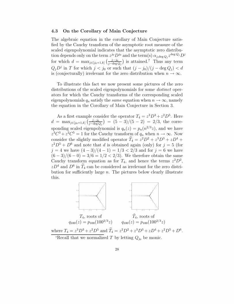
4.3 On the Corollary of Main Conjecture

The algebraic equation in the corollary of Main Conjecture satis-fied by the Cauchy transform of the asymptotic root measure of thescaled eigenpolynomial indicates that the asymptotic zero distribu-tion depends only on the term zj0Dj0 and the term(s) αj,deg Qj

zdeg QjDj

for which d = maxj∈[j0+1,k]

(j−j0

j−deg Qj

)is attained.7 Thus any term

QjDj in T for which j < j0 or such that (j − j0)/(j − degQj) < d

is (conjecturally) irrelevant for the zero distribution when n→ ∞.

To illustrate this fact we now present some pictures of the zerodistributions of the scaled eigenpolynomials for some distinct oper-ators for which the Cauchy transforms of the corresponding scaledeigenpolynomials qn satisfy the same equation when n→ ∞, namelythe equation in the Corollary of Main Conjecture in Section 3.

As a first example consider the operator T4 = z3D3 +z2D5. Hered = maxj∈[j0+1,k]

(j−j0

j−deg Qj

)= (5 − 3)/(5 − 2) = 2/3, the corre-

sponding scaled eigenpolynomial is qn(z) = pn(n2/3z), and we havez3C3 +z2C5 = 1 for the Cauchy transform of qn when n→ ∞. Nowconsider the slightly modified operator T4 = z2D2 + z3D3 + zD4 +z2D5 + D6 and note that d is obtained again (only) for j = 5 (forj = 4 we have (4 − 3)/(4 − 1) = 1/3 < 2/3 and for j = 6 we have(6 − 3)/(6 − 0) = 3/6 = 1/2 < 2/3). We therefore obtain the sameCauchy transform equation as for T4, and hence the terms z2D2,

zD4 and D6 in T4 can be considered as irrelevant for the zero distri-bution for sufficiently large n. The pictures below clearly illustratethis.

-1 -0.5 0 0.5

-1

-0.5

0

0.5

1

-1 -0.5 0 0.5

-1

-0.5

0

0.5

1

T4, roots of T4, roots ofq100(z) = p100(1002/3z) q100(z) = p100(1002/3z)

where T4 = z3D3 + z2D5 and T4 = z2D2 + z3D3 + zD4 + z2D5 +D6.

7Recall that we normalized T by letting Qj0 be monic.

28

However, instead of D6, we may add the more ”disturbing” termzD6 to T4. Note that for the operator T 4 = z2D2 + z3D3 + zD4 +z2D5 + zD6 for j = 6 we have (6 − 3)/(6 − 1) = 3/5 = 0.6 < 2/3.Adding any term QjD

j such that (j−j0)/(j−degQj) < d to a givenoperator, it is clear that the closer the value of (j− j0)/(j−degQj)is to d (in this case 2/3), the more disturbing it is in the sense thatit requires larger n for the corresponding zero distributions to coin-cide. See pictures below, where qn(z) = pn(n2/3z):

-1 -0.5 0 0.5

-1

-0.5

0

0.5

1

-1 -0.5 0 0.5

-1

-0.5

0

0.5

1

-1 -0.5 0 0.5

-1

-0.5

0

0.5

1

T4, roots of T 4, roots of T 4, roots ofq100(z) q100(z) q600(z)

Increasing n however, experiments indicate that the zero distri-butions of the scaled eigenpolynomials of T4 and T 4 coincide, as they(conjecturally) should.

As a second example, consider T5 = z5D5 + z4D6 + z2D8 and

T5 = z2D2 + z5D5 + z4D6 + zD7 + z2D8, whose scaled eigenpolyno-mials qn(z) = pn(n1/2z) both satisfy the Cauchy transform equationz5C5 + z4C6 + z2C8 = 1 when n→ ∞. In the pictures below we seethat the terms z2D2 and zD7 of T5 seem to have no effect on thezero distribution for large n:

-0.6 -0.4 -0.2 0 0.2 0.4 0.6

-1

-0.5

0

0.5

1

-0.6 -0.4 -0.2 0 0.2 0.4 0.6

-1

-0.5

0

0.5

1

T5, roots of q100(z) T5, roots of q100(z)

29

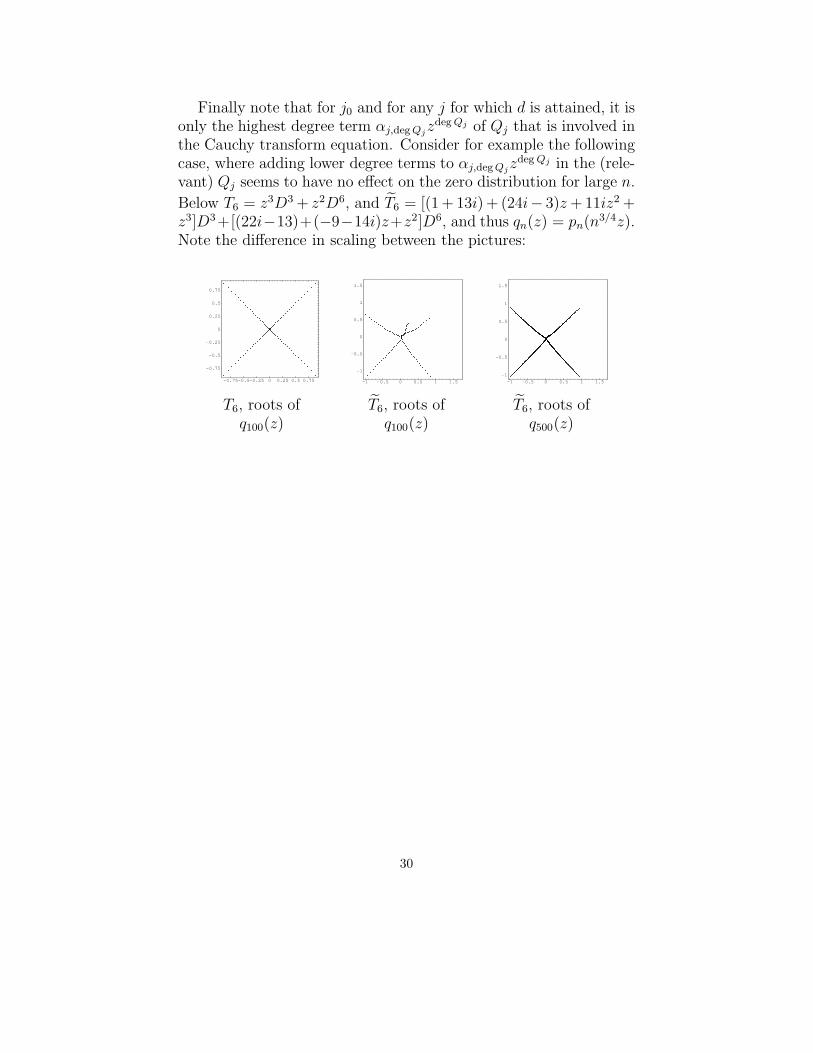
Finally note that for j0 and for any j for which d is attained, it isonly the highest degree term αj,deg Qj

zdeg Qj of Qj that is involved inthe Cauchy transform equation. Consider for example the followingcase, where adding lower degree terms to αj,deg Qj

zdeg Qj in the (rele-vant) Qj seems to have no effect on the zero distribution for large n.

Below T6 = z3D3 + z2D6, and T6 = [(1 + 13i) + (24i− 3)z+ 11iz2 +z3]D3+[(22i−13)+(−9−14i)z+z2]D6, and thus qn(z) = pn(n3/4z).Note the difference in scaling between the pictures:

-0.75-0.5-0.25 0 0.25 0.5 0.75

-0.75

-0.5

-0.25

0

0.25

0.5

0.75

-1 -0.5 0 0.5 1 1.5

-1

-0.5

0

0.5

1

1.5

-1 -0.5 0 0.5 1 1.5

-1

-0.5

0

0.5

1

1.5

T6, roots of T6, roots of T6, roots ofq100(z) q100(z) q500(z)

30

Operator n rn experimental rn conjectured

50 2.7 · 500.967595 c1 · 501

T1 = zD + zD2 + zD3 + zD4 + zD5 100 2.7 · 1000.984180 c1 · 1001

200 2.7 · 2000.992557 c1 · 2001

250 2.7 · 2500.994272 c1 · 2501

50 1.3 · 500.671977 c2 · 505/7

100 1.3 · 1000.694847 c2 · 1005/7

T2 = z2D2 + D7 200 1.3 · 2000.706226 c2 · 2005/7

300 1.3 · 3000.710085 c2 · 3005/7

400 1.3 · 4000.712043 c2 · 4005/7

50 4/3 · 500.469007 c3 · 501/2

100 4/3 · 1000.484824 c3 · 1001/2

T3 = z3D3 + z2D4 + zD5 200 4/3 · 2000.492832 c3 · 2001/2

300 4/3 · 3000.495592 c3 · 3001/2

400 4/3 · 4000.497009 c3 · 4001/2

50 1.4 · 500.633226 c4 · 502/3

100 1.4 · 1000.652141 c4 · 1002/3

T4 = z3D3 + z2D5 200 1.4 · 2000.661412 c4 · 2002/3

300 1.4 · 3000.664511 c4 · 3002/3

400 1.4 · 4000.666066 c4 · 4002/3

50 1.4 · 500.632811 c4 · 502/3

100 1.4 · 1000.651960 c4 · 1002/3

eT4 = z2D2 + z3D3 + zD4 + z2D5 + D6 200 1.4 · 2000.661332 c4 · 2002/3

300 1.4 · 3000.664461 c4 · 3002/3

400 1.4 · 4000.666030 c4 · 4002/3

50 1.5 · 500.462995 c5 · 501/2

100 1.5 · 1000.481684 c5 · 1001/2

T5 = z5D5 + z4D6 + z2D8 200 1.5 · 2000.491066 c5 · 2001/2

300 1.5 · 3000.494304 c5 · 3001/2

400 1.5 · 4000.495971 c5 · 4001/2

50 1.5 · 500.463391 c5 · 501/2

100 1.5 · 1000.481837 c5 · 1001/2

eT5 = z2D2 + z5D5 + z4D6 + zD7 + z2D8 200 1.5 · 2000.491129 c5 · 2001/2

300 1.5 · 3000.494342 c5 · 3001/2

400 1.5 · 4000.495998 c5 · 4001/2

50 1.4 · 500.702117 c6 · 503/4

100 1.4 · 1000.725715 c6 · 1003/4

T6 = z3D3 + z2D6 200 1.4 · 2000.737541 c6 · 2003/4

300 1.4 · 3000.741614 c6 · 3003/4

400 1.4 · 4000.743713 c6 · 4003/4

50 1.4 · 500.769260 c6 · 503/4

eT6 = [(1 + 13i) + (24i − 3)z + 11iz2 + z3]D3 100 1.4 · 1000.760399 c6 · 1003/4

+[(22i − 13) − (9 + 14i)z + z2]D6 200 1.4 · 2000.756161 c6 · 2003/4

300 1.4 · 3000.754590 c6 · 3003/4

400 1.4 · 4000.753765 c6 · 4003/4

31

5 Appendix

5.1 Arriving at the Corollary of Main Conjecture

The algebraic equation in the corollary of Main Conjecture followsimmediately from inserting d as defined in Main Conjecture intoequation (12) in Section 3 and letting n→ ∞. If we put d into (12)we namely get

k∑

j=1

( deg Qj∑

i=0

αj,izi

nmaxj∈[j0+1,k]

(j−j0

j−deg Qj

)(j−i)+j0−j

)Cj(z) = 1. (13)

Denote by Nj,i the exponent of n in (13) for given j and i. Thus

Nj,i = maxj∈[j0+1,k]

(j − j0

j − degQj

)(j − i) + j0 − j.

The terms in (13) for which this exponent is positive tend to zeroas n→ ∞.

First we consider j for which degQj = j, and denote, as usual,by j0 the largest such j. If j = j0, then i ≤ degQj0 = j0 and thusfor j = j0 and i = j0 we get

Nj0,j0 = maxj∈[j0+1,k]

(j − j0

j − degQj

)(j − i) + j0 − j

= maxj∈[j0+1,k]

(j − j0

j − degQj

)(j0 − j0) + j0 − j0 = 0,

and for j = j0 and i < j0 we have

Nj0,i = maxj∈[j0+1,k]

(j − j0

j − degQj

)(j − i) + j0 − j

> maxj∈[j0+1,k]

(j − j0

j − degQj

)(j0 − j0) + j0 − j0 = 0.

Thus Nj0,j0 = 0 and Nj0,i > 0 for i < j0, and for the term corre-sponding to j = j0 in (13) we get

j0∑

i=0

αj0,izi

nmaxj∈[j0+1,k]

(j−j0

j−deg Qj

)(j0−i)+j0−j0

Cj0(z) → zj0Cj0(z)

32

when n→ ∞ (recall that αj0,j0 = 1).Now let j be such that degQj = j and j < j0. Then i ≤ degQj = jand

Nj,j = maxj∈[j0+1,k]

(j − j0

j − degQj

)(j − i) + j0 − j

= maxj∈[j0+1,k]

(j − j0

j − degQj

)(j − j) + j0 − j = j0 − j > 0,

and for i < j we get

Nj,i = maxj∈[j0+1,k]

(j − j0

j − degQj

)(j − i) + j0 − j

> maxj∈[j0+1,k]

(j − j0

j − degQj

)(j − j) + j0 − j = j0 − j > 0,

that is Nj,i > 0 for all j < j0 such that degQj = j and for all i ≤ j.Thus for the corresponding terms in (13) we get

∑

j∈j<j0:deg Qj=j

deg Qj∑

i=0

αj,izi

nmaxj∈[j0+1,j]

(j−j0

j−deg Qj

)(j−i)+j0−j

Cj(z) → 0

when n→ ∞ for every j < j0 for which degQj = j.

Now denote by jm the j for which d = maxj∈[j0+1,k]

(j−j0

j−deg Qj

)is

attained. Note that there may be several distinct j for which thismaximum is attained.8 Then

Njm,degQjm= max

j∈[j0+1,k]

(j − j0

j − degQj

)(j − i) + j0 − j

=

(jm − j0

jm − degQjm

)(jm − degQjm) + j0 − jm

= jm − j0 + j0 − jm = 0,

8Consider for example the Laplace type operator (that is withall polynomial coefficients Qj linear) T = zD + zD2 + . . . zDk.Here j0 = 1 and the equation satisfied by the Cauchy trans-form of the asymptotic root measure of the scaled eigenpolynomialqn(z) = pn(nz) is given by zC(z) + zC2(z) + . . . zCk(z) = 1, sinced = maxj∈[2,k]

(j−j0

j−deg Qj

)= 1 is attained for every j = 2, 3, . . . k.

33

and for i < degQjm we get

Njm,i = maxj∈[j0+1,k]

(j − j0

j − degQj

)(j − i) + j0 − j

>

(jm − j0

jm − degQjm

)(jm − degQjm) + j0 − jm

= jm − j0 + j0 − jm = 0,

i.e. Njm,deg Qjm= 0 and Njm,i > 0 for i < degQjm, and for the term

corresponding to j = jm in (13) we get

deg Qjm∑

i=0

αjm,izi

nmaxj∈[j0+1,k]

(j−j0

j−deg Qj

)(jm−i)+j0−jm

Cjm(z) →

→ αjm,deg Qjmzdeg QjmCjm(z)

when n → ∞. In case of several j for which d is attained, we putA = j : (j−j0)/(j−degQj) = d, and for the corresponding termsin (13) we get

∑

j∈A

deg Qj∑

i=0

αj,izi

nmaxj∈[j0+1,k]

(j−j0

j−deg Qj

)(j−i)+j0−j

Cj(z) →

→∑

j∈A

αj,deg Qjzdeg QjCj(z)

when n → ∞. Now consider the remaining terms in (13), namelyterms for which j < j0 such that degQj < j, terms for whichj0 < j < jm, and terms for which jm < j ≤ k (clearly this lastcase does not exist if jm = k).

We start with j < j0 such that degQj < j. Then i ≤ degQj < jand

Nj,i = maxj∈[j0+1,k]

(j − j0

j − degQj

)(j − i) + j0 − j

> maxj∈[j0+1,k]

(j − j0

j − degQj

)(j − j) + j0 − j = j0 − j > 0,

34

and for the corresponding terms in (13) we have

∑

j∈j<j0:deg Qj<j

deg Qj∑

i=0

αj,izi

nmaxj∈[j0+1,k]

(j−j0

j−deg Qj

)(j−i)+j0−j

Cj(z) → 0

when n→ ∞.

Now assume that jm < k and consider jm < j ≤ k. Clearlyjm > j0 since the maximum is taken over j ∈ [j0+1, k], and thereforei ≤ degQj < j for jm < j ≤ k. Also,

maxj∈[j0+1,k]

(j − j0

j − degQj

)=

(jm − j0

jm − degQjm

)>

(j − j0

j − degQj

),

since the maximum is attained for jm by assumption. Thus we get

Nj,i = maxj∈[j0+1,k]

(j − j0

j − degQj

)(j − i) + j0 − j

=

(jm − j0

jm − degQjm

)(j − i) + j0 − j

>

(j − j0

j − degQj

)(j − i) + j0 − j

≥(

j − j0j − degQj

)(j − degQj) + j0 − j

= j − j0 + j0 − j = 0,

i.e. Nj,i > 0 for every jm < j ≤ k and every i ≤ degQj . For thecorresponding terms in (13) we therefore get

∑

jm<j≤k

deg Qj∑

i=0

αj,izi

nmaxj∈[j0+1,k]

(j−j0

j−deg Qj

)(j−i)+j0−j

Cj(z) → 0

as n→ ∞.

Finally we consider j0 < j < jm. Note that this also covers thecase jm1 < j < jm2 where the maximum d is attained for both jm1

35

and jm2 . Since i ≤ degQj < j we get

Nj,i = maxj∈[j0+1,k]

(j − j0

j − degQj

)(j − i) + j0 − j

=

(jm − j0

jm − degQjm

)(j − i) + j0 − j

>

(j − j0

j − degQj

)(j − i) + j0 − j

≥(

j − j0j − degQj

)(j − degQj) + j0 − j

= j − j0 + j0 − j = 0,

i.e. Nj,i > 0 for every j0 < j < jm and every i ≤ degQj. Thus forthe corresponding terms in (13) we get

∑

j0<j<jm

deg Qj∑

i=0

αj,izi

nmaxj∈[j=+1,k]0

(j−j0

j−deg Qj

)(j−i)+j0−j

Cj(z) → 0

when n→ ∞.

Adding up these results we finally get the following equation byletting n→ ∞ in equation (13):

zj0Cj0(z) +∑

j∈A

αj,deg Qjzdeg QjCj(z) = 1,

where j0 is the largest j for which degQj = j, and A is the setconsisting of all j for which the maximum d = maxj∈[j0+1,k]

(j−j0

j−deg Qj

)

is attained, i.e. A = j : (j − j0)/(j − degQj) = d.

5.2 Theorem 5

Here we prove that for a class of operators containing the opera-tors considered in Corollaries 1 and 2 the conjectured upper boundlimn→∞ sup(rn/n

d) ≤ c1 implies the conjectured lower boundlimn→∞ inf(rn/n

d) ≥ c0 for some constants c1 ≥ c0 > 0 and where dis as in Main Conjecture. This follows automatically from inequality(4) in Lemma 3. We have the following

36

Theorem 5. Let T be a degenerate exactly-solvable operator oforder k which satisfies the condition

b =+

minj∈[1,k−1]

(k − j

k − j + degQj − degQk

)= max

j∈[j0+1,k]

(j − j0

j − degQj

)= d

where the notation min+ means that the minimum is taken onlyover positive values of (k − j + degQj − degQk). Assume that theinequality rn ≤ c1(n−k+1)d holds for some positive constant c1 forall sufficiently large n. Then there exists a positive constant c0 ≤ c1such that rn ≥ c0(n− k+1)d holds for all sufficiently large n. Thus

limn→∞

suprn

nd≤ c1 ⇒ lim

n→∞inf

rn

nd≥ c0.

Proof. From inequality (4) in Lemma 3 we have

1 ≤k−1∑

j=1

deg Qj∑

i=0

|αj,i|2k−j rk−j+i−deg Qkn

(n− k + 1)k−j+

∑

0≤i<deg Qk

|αk,i|rdeg Qk−in

≤k−1∑

j=1

Kjr

k−j+deg Qj−deg Qkn

(n− k + 1)k−j+

∑

0≤i<ik

|αk,i|rik−in

(14)

where the Kj are positive constants. The second sum on the right-hand side of (14) tends to zero when n → ∞ due to Theorem 1.We now decompose the first sum on the right-hand side of (14) intothree parts. Namely, let

A = j : k−jk−j+deg Qj−deg Qk

= d, and note that (k − j + degQj −degQk) > 0 here since d > 0.

B = j : k−jk−j+deg Qj−deg Qk

> d, and note that (k − j + degQj −degQk) > 0 here since d > 0.

C = j : (k−j+degQj−degQk) ≤ 0, and note that j < k in (14).

Clearly due to the condition b = d there are no terms for whichk−j

k−j+deg Qj−deg Qk< d and (k − j + degQj − degQk) > 0 both hold .

37

If j ∈ A then

rk−j+deg Qk−deg Qkn

(n− k + 1)k−j=

(rn

(n− k + 1)d

)k−j+deg Qj−deg Qk

for the corresponding terms in the sum on the right-hand side of(14).

If j ∈ B then d(k − j + degQj − degQk) < (k − j), and thisinequality together with the upper bound rn ≤ c1(n− k+1)d whichwe assume holds for all sufficiently large n, gives us

rk−j+deg Qj−deg Qkn

(n− k + 1)k−j≤ c1(n− k + 1)d(k−j+deg Qj−deg Qk)

(n− k + 1)k−j→ 0

when n→ ∞ for the corresponding terms in (14).

If j ∈ C then (k − j + degQj − degQk) ≤ 0 and we get

rk−j+deg Qj−deg Qkn

(n− k + 1)k−j→ 0

when n → ∞ for the corresponding terms in (14) due to Theorem1. Note that if (k−j+degQj −degQk) = 0 the corresponding termtends to zero when n→ ∞ since j < k in (14).

With this decomposition of the first sum on the right-hand sideof the last inequality in (14) we can write

1 ≤k−1∑

j=1

Kjr

k−j+deg Qj−deg Qkn

(n− k + 1)k−j+

∑

0≤i<ik

|αk,i|rik−in

≤∑

j∈A

Kj

(rn

(n− k + 1)d

)k−j+deg Qj−deg Qk

+∑

j∈B

Kjc1(n− k + 1)d(k−j+deg Qj−deg Qk)

(n− k + 1)k−j

+∑

j∈C

Kjr

k−j+deg Qj−deg Qkn

(n− k + 1)k−j+

∑

0≤i<ik

|αk,i|rik−in

38

where the last three sums tend to zero when n → ∞ by the abovearguments (and the last one due to Theorem 1).Thus for all sufficiently large n there exists a positive constant c′

such that

c′ ≤∑

j∈A

Kj

(rn

(n− k + 1)d

)k−j+deg Qj−deg Qk

(15)

where c′ → 1 when n → ∞. If the set A contains precisely oneelement, then the sum in (15) consists of one single term, and we aredone: there exists a positive constant c0 = (c′/Kj)

1/(k−j+deg Qj−deg Qk)

such that rn ≥ c0(n − k + 1)d for all sufficiently large n, and thuslimn→∞ inf(rn/n

d) ≥ c0.But clearly, for some operators A will contain more than one ele-

ment. If this is the case define m := minj∈A(k−j+degQj −degQk)and denote by jm the corresponding j for which this minimum is at-tained. Using the upper bound rn ≤ c1(n− k + 1)d we then get thefollowing inequality from (15):

c′ ≤∑

j∈A

Kj

(rn

(n− k + 1)d

)k−j+deg Qj−deg Qk

= Kjm

(rn

(n− k + 1)d

)m

+∑

j∈A\jm

Kj

(rn

(n− k + 1)d

)m(rn

(n− k + 1)d

)k−j+deg Qj−deg Qk−m

≤ Kjm

(rn

(n− k + 1)d

)m

+∑

j∈A\jm

Kj

(rn

(n− k + 1)d

)m

ck−j+deg Qj−deg Qk−m1

=

(rn

(n− k + 1)d

)m(Kjm +

∑

j∈A\jm

Kj · ck−j+deg Qj−deg Qk−m1

)

=

(rn

(n− k + 1)d

)m

·K

where K > 0. Thus rn ≥(

c′

K

)1/m(n−k+1)d for all sufficiently large

n, and therefore there exists a positive constant c0 = (1/K)1/m (re-call that c′ → 1 when n→ ∞) such that limn→∞ inf rn

nd ≥ c0.

39

Remark. About the last inequality following from (15) in the aboveproof, consider for example the operator T = zD+D2 +zD3 +zD4.In this case, by Lemma 3, we have

1 ≤3∑

j=1

24−jr3−j+deg Qjn

(n− 3)4−j= 8

r3n

(n− 3)3+ 4

rn

(n− 3)2+ 2

rn

(n− 3),

where rn is the largest modulus of all roots of the unique and moniceigenpolynomial of T . For this operator d = 1 and we see that(4− j)/(3− j+degQj) = d for j = 1 and for j = 3. Now, assumingthat rn ≤ c1(n − 3) holds for some positive constant c1 for large n,our inequality becomes

1 ≤ 8r3n

(n− 3)3+ 4

rn

(n− 3)2+ 2

rn

(n− 3)

≤ 8rn

(n− 3)· c

21(n− 3)2

(n− 3)2+ 4

c1(n− 3)

(n− 3)2+ 2

rn

(n− 3)

= (8c21 + 2)rn

(n− 3)+

4c1(n− 3)

where the last term tends to zero as n → ∞. Thus rn ≥ c0(n − 3)for sufficiently large choices on n, where c0 = 1/(8c21 +2), and hencelimn→∞ inf(rn/n) ≥ c0.

6 Open Problems

1. The main challenge is to obtain a complete proof of the MainConjecture, see Introduction. This proof requires both the sharpupper and lower bounds of the largest root. The upper bound canapparently be obtained by a detailed study of the correspondingRiccati equation at ∞. If the Main Conjecture is settled then toachieve its corollary (the Cauchy transform equation) one can usea technique similar to that of [2] to prove the basic assumption, seeSection 3.

2. As suggested by one of the referees, estimates similar to thatof Main Conjecture can be formulated for the sequence of roots zn,i

of pn such that limn→∞rn,i

rn,n= α where 0 < α < 1 and |zn,i| = rn,i.

40

3. In the case of orthogonal polynomials there is a number of re-sults describing the growth of the largest modulus rn of the rootsas an expansion in powers of n, see e.g. [11] and [12] and referencestherein. In the present paper we conjectured the form of the leadingterm of rn in our more general setup. As suggested by one of thereferees, the question about the lower terms in the expansion of rn

is natural in our context as well.

4. Operators of the type we consider occur in the theory of Bochner-Krall orthogonal systems, i.e. families of polynomials which are botheigenfunctions of some finite order differential operator and orthog-onal with respect to some suitable inner product. A lot is knownabout the asymptotic zero distribution of orthogonal polynomials,and by comparing such known results with results on the asymptoticzero distribution of eigenpolynomials of degenerate exactly-solvableoperators, we believe it will be possible to gain new insight into thenature of BKS. We have previously used our results from [2] to provea special case of a general conjecture describing the leading terms ofall Bochner-Krall operators, see [3]. Another problem relevant forBKS is to describe all exactly-solvable operators whose eigenpoly-nomials have real roots only.

5. Numerical evidence indicates that the roots of the scaled eigen-polynomials fill certain curves in the complex plane. The supportof the limiting root measure µ seems to be a tree. This is the casefor the non-degenerate exactly-solvable operators which we treatedin [2], but then without such a scaling of the eigenpolynomials. Bya tree we mean a connected compact subset Γ of C which consistsof a finite union of analytis curves and where C \ Γ is simply con-nected. The (conjectural) algebraic equation satisfied by the Cauchytransform contains a lot of information about µ, and it remains todescribe its support explicitly.

6. Conjecturally the support of the asymptotic zero distributionof the scaled eigenpolynomial qn is the union of a finite number ofanalytic curves in the complex plane which we denote by ΞT , i.e.ΞT = supp µ, where µ is the limiting root measure of qn. Then the

41

following conjecture seems to be quite plausible9.

Conjecture 1. [Interlacing property] For any family qn of ap-propriately scaled eigenpolynomials of a degenerate exactly-solvableoperator, the zeros of any two consecutive polynomials qn+1 and qninterlace along ΞT for all sufficiently large integers n.

When defining the interlacing property some caution is requiredsince the zeros of qn do not lie exactly on ΞT . Thus identify somesufficiently small neighbourhood N(ΞT ) of ΞT with the normal bun-dle to ΞT by equipping N(ΞT ) with the projection onto ΞT alongthe fibres which are small curvilinear segments orthogonal to ΞT .We then say that two sets of points in N(ΞT ) interlace if their or-thogonal projections on ΞT interlace in the usual sense. If ΞT hassingularities one should first remove some sufficiently small neigh-bourhoods of these singularities and then proceed as above on theremaining part of ΞT . Conjecture 1 thus states that for any suffi-ciently small neighbourhood N(ΞT ) of ΞT there exists a number n0

such that the interlacing property holds for the zeros of qn and qn+1

for all n ≥ n0. We conclude this section by showing some picturesillustrating the interlacing property. Below, small dots represent theroots of qn+1 and large dots represent the roots of qn for some fixedn.

-0.6 -0.4 -0.2 0 0.2 0.4 0.6-0.6

-0.4

-0.2

0

0.2

0.4

0.6

-1 -0.75-0.5-0.25 0 0.25 0.5-1

-0.5

0

0.5

1

T = z2D2 + z3D3 + zD5 , T = zD + z2D2 +D3 ,roots of q25 and q24. roots of q20 and q19.

9The question concerning interlacing was raised by B. Shapiro.Also see [1].

42

-1.75-1.5-1.25 -1 -0.75-0.5-0.25 0

-0.75

-0.5

-0.25

0

0.25

0.5

0.75

-0.8 -0.6 -0.4 -0.2 0 0.2 0.4

-0.6

-0.4

-0.2

0

0.2

0.4

0.6

T = zD + zD2 + zD3 + zD4 + zD5, T = z3D3 + z2D5 + zD6,roots of q23 and q22. roots of q20 and q19.

References

[1] C.M. Bender, S. Boettcher and V.M. Savage: Conjecture onthe interlacing of zeros in complex Sturm-Liouville problem, J.Math. Phys. 41 (2000), 6381-6387.

[2] T. Bergkvist and H. Rullgard: On polynomial eigenfunctionsfor a class of differential operators, Math. Research Letters 9,153 – 171 (2002).

[3] T. Bergkvist, H. Rullgard and B. Shapiro: On Bochner-KrallOrthogonal Polynomial Systems, Math.Scand 94, no. 1, 148-154 (2004).

[4] T. Bergkvist: On generalized Laguerre Polynomials withReal and Complex Parameter, Research Reports in Math-ematics, Stockholm University No. 2 (2003), available athttp://www.math.su.se/reports/2003/2/.

[5] J. Borcea, R. Bøgvad, B. Shapiro: On Rational Approximationof Algebraic Functions, Adv. Math 204 (2006), 448-480.

[6] H. Dette, W. Studden: Some new asymptotic properties for thezeros of Jacobi, Laguerre and Hermite polynomials, Construc-tive Approx. 11 (1995).

[7] W. N. Everitt, K. H. Kwon, L. L. Littlejohn and R. Wellman:Orthogonal polynomial solutions of linear ordinary differentialequations, J. Comp. Appl. Math 133, 85–109 (2001).

43

[8] J. Faldey, W. Gawronski: On the limit distribution of the ze-ros of Jonquire polynomials and generalized classical orthogo-nal polynomials, Journal of Approximation Theory 81,231-249(1995).

[9] W. Gawronski: On the asymptotic distribution of the zeros ofHermite, Laguerre and Jonquire polynomials, J. Approx. The-ory 50 (1987), p. 214-231

[10] A. Gonzalez-Lopez, N. Kamran, P.J. Olver: Normalizabilityof One-dimensional Quasi-exactly Solvable Schrodinger Opera-tors, Comm. Math. Phys. 153 (1993), no 1, p.117-146.

[11] I. Krasikov: On the zeros of polynomials and allied functionssatisfying second order differential equations, East J. Approx.9 (2003), no.1, 51-65.

[12] I. Krasikov: Bounds for zeros of the Laguerre polynomials, J.Approx. Theory 121 (2003), no.2, 287-291.

[13] A.B.J. Kujilaars, K.T-R McLaughlin: Asymptotic zero be-haviour of Laguerre polynomials with negative parameter, Con-str. Approx. 20 (2004), no. 4, 497-523.

[14] K. H. Kwon, L. L. Littlejohn and G. J. Yoon: Bochner-Krallorthogonal polynomials, Special functions, 181–193, World Sci.Publ., River Edge, NJ, (2000).

[15] Littlejohn: Lecture Notes in Mathematics 1329 ed M Alfaro etal (Berlin: Springer), p. 98.

[16] G. Masson and B. Shapiro: A note on polynomial eigenfunc-tions of a hypergeometric type operator, Experimental Mathe-matics, 10, 609–618.

[17] A. Martinez-Finkelshtein, P. Martinez-Gonzalez, A. Zarzo:WKB approach to zero distribution of solutions of linear secondorder differential equations, J. Comp. Appl. Math. 145 (2002),167-182.

[18] A. Martinez-Finkelshtein, P. Martinez-Gonzalez, R. Orive: Onasymptotic zero distribution of Laguerre and generalized Besselpolynomials with varying parameters. Proceedings of the FifthInternational Symposium on Orthogonal Polynomials, Special

44

Functions and their Applications (Patras 1999), J. Comput.Appl. Math. 133 (2001), no. 1-2, p. 477-487.

[19] A. Turbiner: Lie-Algebras and Linear Operators with InvariantSubspaces, Lie Algebras, Cohomologies and New Findings inQuantum Mechanics AMS Contemporary Mathematics’ series,N. Kamran and P. Olver (Eds.), vol 160, 263-310 (1994).

[20] A. Turbiner: On Polynomial Solutions of differential equations,J. Math. Phys. 33 (1992) p.3989-3994.

[21] A. Turbiner: Lie algebras and polynomials in one variable, J.Phys. A: Math. Gen. 25 (1992) L1087-L1093.

45

PAPER V

On Roots of Eigenpolynomials forDegenerate Exactly-Solvable Differential

Operators

Tanja Bergkvist & Jan-Erik Bjorksubmitted

Abstract

In this paper we partially settle our conjecture from [1]on the roots of eigenpolynomials for degenerate exactly-solvable operators. Namely, for any such operator we es-tablish a lower bound (which supports our conjecture) forthe largest modulus of all roots of its unique and moniceigenpolynomial pn as the degree n tends to infinity. Themain theorem below thus extends earlier results obtainedin [1] for a restrictive class of operators.

1 Introduction

We are interested in roots of eigenpolynomials satisfying certainlinear differential equations. Namely, consider an operator

T =

k∑

j=1

QjDj

where D = d/dz and the Qj are complex polynomials in one vari-able satisfying the condition degQj ≤ j, with equality for at leastone j, and in particular degQk < k for the leading term. Such op-erators are referred to as degenerate exactly-solvable operators1, see[1]. We are interested in eigenpolynomials of T , that is polynomialssatisfying

T (pn) = λnpn (1)

for some value of the spectral parameter λn, where n is a positive in-teger and deg pn = n. The importance of studying eigenpolynomialsfor these operators is among other things motivated by numerous

1Correspondingly, operators for which degQk = k are called non-degenerate exactly-solvable operators. We have treated roots ofeigenpolynomials for these operators in [2].

1

examples coming from classical orthogonal polynomials, such as theLaguerre and Hermite polynomials, which appear as solutions to (1)for certain choices on the polynomials Qj when k = 2. Note howeverthat for the operators considered here the sequence of eigenpolyno-mials pn is in general not an orthogonal system.

Let us briefly recall our previous results:

A. In [2] we considered eigenpolynomials of non-degenerate exactly-solvable operators, that is operators of the above type but with thecondition degQk = k for the leading term. We proved that whenthe degree n of the unique and monic eigenpolynomial pn tends toinfinity, the roots of pn stay in a compact set in C and are distributedaccording to a certain probability measure which is supported by atree and which depends only on the leading polynomial Qk.

B. In [1] we studied eigenpolynomials of degenerate exactly-solvableoperators (degQk < k). We proved that there exists a unique andmonic eigenpolynomial pn for all sufficiently large values on the de-gree n, and that the largest modulus of the roots of pn tends toinfinity when n→ ∞. We also presented an explicit conjecture andpartial results on the growth of the largest root. Namely,

Conjecture (from [1]). Let T =∑k

j=1QjDj be a degenerate

exactly-solvable operator of order k and denote by j0 the largest jfor which degQj = j. Let rn = max|α| : pn(α) = 0, where pn isthe unique and monic nth degree eigenpolynomial of T . Then

limn→∞

rn

nd= c0,

where c0 > 0 is a positive constant and

d := maxj∈[j0+1,k]

(j − j0

j − degQj

).

Extensive computer experiments listed in [1] confirm the exis-tence of such a constant c0. Now consider the scaled eigenpolyno-mial qn(z) = pn(ndz). We construct the probability measure µn byplacing a point mass of size 1/n at each zero of qn. Numerical ev-idence indicates that for each degenerate exactly-solvable operator

2

T , the sequence µn converges weakly to a probability measure µT

which is (compactly) supported by a tree. In [1] we deduced the al-gebraic equation satisfied by the Cauchy transform of µT .2 Namely,let

T =

k∑

j=1

Qj(z)Dj =

k∑

j=1

( deg Qj∑

i=0

qj,izi)Dj

and denote by j0 the largest j for which degQj = j. Assumingwithout loss of generality that Qj0 is monic, i.e. qj0,j0 = 1, we have

zj0Cj0(z) +∑

j∈A

qj,deg Qjzdeg QjCj(z) = 1

where C(z) =∫ dµT (ζ)

z−ζis the Cauchy transform of µT and A = j :

(j − j0)/(j − degQj) = d, where d is defined in the conjecture.

Below we present some typical pictures of the distribution of rootsof the scaled eigenpolynomial qn(z) = pn(ndz) for some degenerateexactly-solvable operators.

Fig.1: Fig.2: Fig.3:

-2 -1.5 -1 -0.5 0-1.5

-1

-0.5

0

0.5

1

1.5

-1 -0.5 0 0.5 1

-1

-0.5

0

0.5

1

-0.4 -0.2 0 0.2 0.4

-1

-0.5

0

0.5

1

roots of roots of roots ofq100(z) = p100(100z) q100(z) = p100(100z) q100(z) = p100(100z)

Fig.1: T1 = zD + zD2 + zD3 + zD4 + zD5.Fig.2: T2 = z2D2 +D7.Fig.3: T3 = z3D3 + z2D4 + zD5.

In this paper we extend the results from [1] by establishing alower bound for the largest modulus rn of the roots of pn for anydegenerate exactly-solvable operator and which supports the above

2It remains to prove the existence of µT and to describe its supportexplicitly, see Open Problems and Conjectures.

3

conjecture.3 This is our main result:

Main Theorem. Let T =∑k

j=1QjDj be a degenerate exactly-

solvable operator and denote by j0 the largest j for which degQj = j.Let pn be the unique and monic nth degree eigenpolynomial of T andrn = max|α| : pn(α) = 0. Then there exists an integer n0 and apositive constant s > 0 such that

rn ≥ s · nd

for all n > n0, where

d := maxj∈[j0+1,k]

( j − j0j − degQj

).

Acknowledgements. The authors are greatly obliged to ProfessorBoris Shapiro for introducing us to this very fascinating subject.Our research was supported by Stockholm University.

2 Proofs

Lemma 1. For any monic polynomial p(z) of degree n ≥ 2 forwhich all the zeros are contained in a disc of radius A ≥ 1, thereexists an integer n(j) and an absolute constant Cj depending onlyon j, such that for every j ≥ 1 and every n ≥ n(j) we have

1

Cj

· nj

Aj≤

∣∣∣∣∣∣∣∣p(j)(z)

p(z)

∣∣∣∣∣∣∣∣2A

≤ Cj ·nj

Aj(2)

where p(j)(z) denotes the jth derivative of p(z), and where we haveused the maximum norm ||p(z)||2A = max|z|=2A |p(z)|.

Remark. The right-hand side of the above inequality actually holdsfor all n ≥ 2, whereas the left-hand side holds for all n ≥ n(j).

Proof. To obtain the inequality on the right-hand side we use thenotation p(z) =

∏ni=1(z−αi) where by assumption |αi| ≤ A for every

complex root of p(z). Then p(j)(z) is the sum of n(n−1) · · · (n−j+1)

3It is still an open problem to prove the upper bound.

4

terms, each being the product of (n − j) factors (z − αi).4 Thus

p(j)(z)/p(z) is the sum of n(n− 1) · · · (n− j + 1) terms, each equalto 1 divided by a product consisting of n − (n − j) = j factors(z − αi). If |z| = 2A we get |z − αi| ≥ A⇒ 1

|z−αi|≤ 1

A, and thus

∣∣∣∣p(j)

p

∣∣∣∣2A

≤ n(n− 1) · · · (n− j + 1)

Aj≤ Cj ·

nj

Aj.

Here we can choose Cj = 1 for all j, but we refrain from doing thissince we will need Cj large enough to obtain the constant 1/Cj inthe left-hand side inequality. To prove the left-hand side inequalitywe will need inequalities (i)-(iv) below, where we need (i) to prove(ii), and we need (ii) and (iii) to prove (iv), from which the left-handside inequality of this lemma follows.

For every j ≥ 1 we have

(i)∣∣∣∣ d

dz

(p(j)(z)p(z)

)∣∣∣∣2A

≤ j · nj

Aj+1 .

For every j ≥ 1 there exists a positive constant C ′j depending only

on j, such that

(ii)

∣∣∣∣∣∣∣∣p(j)

p− (p′)j

pj

∣∣∣∣∣∣∣∣2A

≤ C ′j · nj−1

Aj .

(iii)∣∣∣∣p′

p

∣∣∣∣2A

≥ n3A

.

For every j ≥ 1 there exists a positive constant C ′′j and some in-

teger n(j) such that for all n ≥ n(j) we have

(iv)∣∣∣∣ p(j)

p

∣∣∣∣2A

≥ C ′′j · nj

Aj .

To prove (i), let p(z) =∏n

i=1(z − αi), where |αi| ≤ A for eachcomplex root αi of p(z). Then again p(j)(z)/p(z) is the sum ofn(n − 1) · · · (n − j + 1) terms and each term equals 1 divided by aproduct consisting of j factors (z − αi). Differentiating each such

4Differentiating p(z) =∏n

i=1(z − αi) once yields(

n1

)= n terms

each term being a product of (n−1) factors (z−αi), differentiatingonce again we obtain n

(n−1

1

)= n(n − 1) terms, each being the

product of (n− 2) factors (z − αi), etc.

5

term we obtain a sum of j terms each being on the form (−1) divided

by a product consisting of (j + 1) factors (z −αi).5 Thus d

dz

(p(j)(z)p(z)

)

is a sum consisting of j · n(n− 1) · · · (n− j + 1) terms, each on theform (−1) divided by (j + 1) factors (z − αi). Using 1

|z−αi|≤ 1

Afor

|z| = 2A since |αi| ≤ A for all i ∈ [1, n], we thus get

∣∣∣∣ ddz

(p(j)(z)

p(z)

)∣∣∣∣2A

≤ j · n(n− 1) · · · (n− j + 1)

Aj+1≤ j · nj

Aj+1.

To prove (ii) we use (i) and induction over j. The case j = 1 is trivial

since p′

p− (p′)1

p1 = 0. If we put j = 1 in (i) we get∣∣∣∣ d

dz

(p′

p

)∣∣∣∣2A

≤ nA2 .

But ddz

(p′

p

)= p(2)

p− (p′)2

p2 , and thus∣∣∣∣p(2)

p− (p′)2

p2

∣∣∣∣ ≤ nA2 , so (ii) holds

for j = 2. We now proceed by induction. Assume that (ii) holds for

some j = p ≥ 2, i.e.∣∣∣∣p(p)

p− (p′)p

pp

∣∣∣∣2A

≤ C ′p · np−1

Ap . Also note that

with j = p in (i) we have

∣∣∣∣p(p+1)

p− p(p) · p′

p2

∣∣∣∣2A

=∣∣∣∣ ddz

(p(p)

p

)∣∣∣∣2A

≤ p · np

Ap+1,

and also ||p′p||2A ≤ n

A(from the right-hand side inequality of this

lemma). Thus we have∣∣∣∣

∣∣∣∣p(p+1)

p− (p′)p+1

pp+1

∣∣∣∣

∣∣∣∣2A

=

∣∣∣∣

∣∣∣∣p(p+1)

p− p(p) · p′

p2+p(p) · p′p2

− (p′)p+1

pp+1

∣∣∣∣

∣∣∣∣2A

≤∣∣∣∣∣∣∣∣p(p+1)

p− p(p) · p′

p2

∣∣∣∣∣∣∣∣2A

+

∣∣∣∣∣∣∣∣p′

p

(p(p)

p− (p′)p

pp

)∣∣∣∣∣∣∣∣2A

≤ p · np

Ap+1+n

A· C ′

p ·np−1

Ap

= (p+ C ′p) ·

np

Ap+1= C ′

p+1 ·np

Ap+1.

5With D = d/dz consider for example D 1Qj

i=1(z−αi)=

−1·DQj

i=1(z−αi)Qj

i=1(z−αi)2, which is a sum of j terms, each being on the form

(−1) divided by a product consisting of 2j−(j−1) = (j+1) factors(z − αi).

6

To prove (iii) observe that p′(z)p(z)

=∑n

i=11

(z−αi)=

∑ni=1

1z· 1

1−αiz

. By

assumption |αi| ≤ A for all complex roots αi of p(z), so for |z| = 2Awe have |αi

z| ≤ A

2A= 1

2for all i ∈ [1, n]. Writing wi = 1

1−αiz

we obtain

|wi − 1| =

∣∣∣∣1

1 − αi

z

− 1 − αi

z

1 − αi

z

∣∣∣∣ =

∣∣αi

z

∣∣∣∣1 − αi

z

∣∣ ≤ 1

2|wi|,

which implies

Re

(1

1 − αi

z

)= Re(wi) ≥

2

3∀i ∈ [1, n] ⇒ Re

( n∑

i=1

1

1 − αi

z

)≥ 2n

3.

Thus∣∣∣∣∣∣∣∣p′(z)

p(z)

∣∣∣∣∣∣∣∣2A

= max|z|=2A

∣∣∣∣p′(z)

p(z)

∣∣∣∣ = max|z|=2A

1

|z| ·∣∣∣∣

n∑

i=1

1

1 − αi

z

∣∣∣∣

≥ 1

2A·∣∣∣∣

n∑

i=1

1

1 − αi

z

∣∣∣∣2A

≥ 1

2A· Re

( n∑

i=1

1

1 − αi

z

)

≥ n

3A.

To prove (iv) we note that from (iii) we obtain∣∣∣∣(p′

p

)j∣∣∣∣2A

≥ nj

3jAj ,

and this together with (ii) yields

∣∣∣∣∣∣∣∣p(j)

p

∣∣∣∣∣∣∣∣2A

=

∣∣∣∣∣∣∣∣(p′

p

)j

+p(j)

p−

(p′

p

)j∣∣∣∣∣∣∣∣2A

≥∣∣∣∣∣∣∣∣(p′

p

)j∣∣∣∣∣∣∣∣2A

−∣∣∣∣∣∣∣∣p(j)

p−

(p′

p

)j∣∣∣∣∣∣∣∣2A

≥ nj

3jAj− C ′

j ·nj−1

Aj=nj

Aj

(1

3j−C ′

j

n

)≥ C ′′

j · nj

Aj,

where C ′′j is a positive constant such that C ′′

j ≤(

13j − C′

j

n

)for all

n ≥ n(j). The left-hand side inequality in this lemma now followsfrom (iv) if we choose the constant Cj on right-hand side inequalityso large that 1

Cj≤ C ′′

j .

7

To prove Main Theorem we will need the following lemma, whichfollows from Lemma 1:

Lemma 2. Let 0 < s < 1 and d > 0 be real numbers. Let p(z)be any monic polynomial of degree n ≥ 2 such that all its zeros arecontained in a disc of radius A = s · nd, and let Qj(z) be arbitrarypolynomials. Then there exists some positive integer n0 and positiveconstants Kj such that

1

Kj

·nd(deg Qj−j)+j ·sdeg Qj

sj≤

∣∣∣∣∣∣∣∣Qj(z)·

p(j)

p

∣∣∣∣∣∣∣∣2snd

≤ Kj·nd(deg Qj−j)+j·sdeg Qj

sj

for every j ≥ 1 and all n ≥ max(n0, n(j)), where n(j) is as in Lemma1.

Proof. Let Qj(z) =∑deg Qj

i=0 qj,izi. Then for |z| = 2A >> 1 we

have

|Q(z)|2A = |qj,deg Qj|2deg QjAdeg Qj

(1 +O(

1

A)

).

Since A = s · nd there exists some integer n0 such that n ≥ n0 ⇒A ≥ A0 >> 1, and thus by Lemma 1 there exists a positive constantKj such that the following inequality holds for all n ≥ max(n(j), n0)and all j ≥ 1:

1

Kj· n

j

Aj· Adeg Qj ≤

∣∣∣∣∣∣∣∣Qj(z) ·

p(j)

p

∣∣∣∣∣∣∣∣2A

≤ Kj ·nj

Aj·Adeg Qj .

Inserting A = s · nd in this inequality we obtain

1

Kj· nj

sjndj·sdeg Qjnd·deg Qj ≤

∣∣∣∣∣∣∣∣Qj(z)·

p(j)

p

∣∣∣∣∣∣∣∣2snd

≤ Kj·nj

sjndj·sdeg Qjnd·deg Qj

⇔1

Kj·nd(deg Qj−j)+j ·s

deg Qj

sj≤

∣∣∣∣∣∣∣∣Qj(z)·

p(j)

p

∣∣∣∣∣∣∣∣2snd

≤ Kj·nd(deg Qj−j)+j·sdeg Qj

sj

for every j ≥ 1 and all n ≥ max(n0, n(j)).

Proof of Main Theorem. Let d = maxj∈[j0+1,k]

(j−j0

j−deg Qj

)where

8

j0 is the largest j for which degQj = j in the degenerate exactly-

solvable operator T =∑k

j=1QjDj, where Qj(z) =

∑deg Qj

i=0 qj,izi.

Let pn(z) be the nth degree unique and monic eigenpolynomial of Tand denote by λn the corresponding eigenvalue. Then the eigenvalueequation can be written

k∑

j=1

Qj(z) ·p

(j)n (z)

pn(z)= λn (3)

where λn =∑j0

j=1 qj,j · n!(n−j)!

. We will now use the result in Lemma

2 to estimate each term in (3).

* Denote by jm the largest j for which d is attained. Then d =(jm − j0)/(jm − degQjm) ⇒ d(degQjm − jm) + jm = j0, and jm −degQjm = (jm − j0)/d. By Lemma 2 we have:

1

Kjm

· nj0 · 1

sjm−j0

d

≤∣∣∣∣∣∣∣∣Qjm(z) · p

(jm)

p

∣∣∣∣∣∣∣∣2snd

≤ Kjm · nj0 · 1

sjm−j0

d

. (4)

Note that the exponent of s is positive since jm > j0 and d > 0.In what follows we will only need the left-hand side of the aboveinequality.

* Consider the remaining (if there are any) j0 < j < jm forwhich d is attained. For such j we have (using the right-hand sideinequality of Lemma 2):

∣∣∣∣

∣∣∣∣Qj(z) ·p(j)

p

∣∣∣∣

∣∣∣∣2snd

≤ Kjnj0 · 1

sj−j0

d

= Kjnj0 · 1

sjm−j0

d

· s jm−jd

≤ Kjnj0 · 1

sjm−j0

d

· s1/d (5)

where we have used that (jm − j) ≥ 1 and s < 1 ⇒ s(jm−j)/d ≤ s1/d.

* Consider all j0 < j ≤ k for which d is not attained. Then(j−degQj) > 0 and (j−j0)/(j−degQj) < d⇒ d(degQj−j)+j < j0and we can write d(degQj − j) + j ≤ j0 − δ where δ > 0. Then we

9

have:∣∣∣∣∣∣∣∣Qj(z) ·

p(j)

p

∣∣∣∣∣∣∣∣2snd

≤ Kj · nd(deg Qj−j)+j · sdeg Qj

sj≤ Kj · nj0−δ · s

deg Qj

sj

≤ Kj · nj0−δ · 1

sk, (6)

where the last inequality follows since degQj ≥ 0 ⇒ sdeg Qj ≤ s0 = 1and j ≤ k ⇒ sj ≥ sk since 0 < s < 1.

* For j = j0 by definition degQj0 = j0 and thus:∣∣∣∣∣∣∣∣Qj0(z) ·

p(j0)

p

∣∣∣∣∣∣∣∣2snd

≤ Kj0 ·nd(deg Qj0−j0)+j0 · s

deg Qj0

sj0= Kj0 ·nj0. (7)

* Now consider all 1 ≤ j ≤ j0−1. Since n ≥ n0 ⇒ A = snd >> 1we get (snd)j−deg Qj ≥ 1 and thus:∣∣∣∣∣∣∣∣Qj(z) ·

p(j)

p

∣∣∣∣∣∣∣∣2snd

≤ Kj · nd(deg Qj−j)+j · sdeg Qj

sj= Kj · nj · (snd)(deg Qj−j)

= Kj · nj · 1

(snd)j−deg Qj≤ Kj · nj ≤ Kj · nj0−1. (8)

* Finally we estimate the eigenvalue λn =∑j0

i=1 qj,j · n!(n−j)!

, which

grows as nj0 for large n, since there exists an integer nj0 and somepositive constant K ′

j0 such that for all n ≥ nj0 we obtain:

|λn| ≤j0∑

j=1

|qj,j| ·n!

(n− j)!

= |qj0,j0| ·n!

(n− j0)!

[1 +

∑

1≤j<j0

∣∣∣∣qj,jqj0,j0

∣∣∣∣ ·(n− j0)!

(n− j)!

]

≤ K ′j0· nj0 . (9)

Finally we rewrite the eigenvalue equation (3) as follows:

Qjm(z) · p(jm)n (z)

pn(z)= λn +

∑

j 6=jm

Qj(z)p

(j)n (z)

pn(z).

10

Applying inequalities (5)-(9) to this we obtain

∣∣∣∣∣∣∣∣Qjm · p

(jm)n (z)

pn(z)

∣∣∣∣∣∣∣∣2snd

≤ |λn| +∑

j 6=jm

∣∣∣∣∣∣∣∣Qj

p(j)n (z)

pn(z)

∣∣∣∣∣∣∣∣2snd

≤ K ′j0n

j0 +Kj0nj0 +

∑

1≤j<j0

Kjnj0−1

+∑

j0<j≤k

(j−j0

j−deg Qj)<d

Kjnj0−δ

sk+

∑

j0<j<jm

(j−j0

j−deg Qj)=d

Kjnj0

s1/d

sjm−j0

d

≤ K · nj0 +K · nj0−δ

sk+K · nj0

s1/d

sjm−j0

d

(10)

for all n ≥ max(n0, n(j), nj0), where K is some positive constantand 0 < s < 1. For the term on the left-hand side of the rewritteneigenvalue equation above we obtain using (4) the following estima-tion:

1

K· nj0 · 1

sjm−j0

d

≤ 1

Kjm

· nj0 · 1

sjm−j0

d

≤∣∣∣∣∣∣∣∣Qjm · p

(jm)n (z)

pn(z)

∣∣∣∣∣∣∣∣2snd

(11)

for some constantK ≥ Kjm which also satisfies (10). Now combining(10) and (11) we get

1

K· nj0 · 1

sjm−j0

d

≤ K · nj0 +K · nj0−δ

sk+K · nj0

s1/d

sjm−j0

d

.

Dividing this inequality by nj0 and multiplying by K we have

1

sjm−j0

d

≤ K2 +K2 · 1

nδ· 1

sk+K2 · s1/d

sjm−j0

d

.

⇔1

sw≤ K2 +

K2

sk· 1

nδ+K2 · s

1/d

sw

⇔1

sw[1 −K2 · s1/d] ≤ K2 +

K2

sk· 1

nδ. (12)

where w = (jm − j0)/d > 0.

11

In what follows we will obtain a contradiction to this inequalityfor some small properly chosen 0 < s < 1 and all sufficiently largen. Since jm ∈ [j0 + 1, k] we have w = (jm − j0)/d ≥ 1/d, and sinces < 1 we get sw ≤ s1/d ⇒ 1/sw ≥ 1/s1/d. Now choose s1/d = 1

4K2 ,where K is the constant in (12). Then estimating the left-handside of (12) we get

1

sw[1 −K2 · s1/d] ≥ 1

s1/d[1 −K2 · s1/d] = 4K2 −K2 = 3K2

and thus from (12) we have

3K2 ≤ 1

sw[1 −K2 · s1/d] ≤ K2 +

K2

sk· 1

nδ

⇔

2K2 ≤ K2

sk· 1

nδ

⇔nδ ≤ 1

2· 1

sk=

1

2(2K)2dk.

We therefore obtain a contradiction to this inequality, and henceto inequality (12) and thus to the eigenvalue equation (3), if nδ >12(2K)2dk and s = 1/(2K)2d, and consequently all roots of pn cannot

be contained in a disc of radius s · nd for such choices on s and n.Hence there exists an integer n0 such that for all n > n0 we havern > s · nd.

3 Open Problems and Conjectures

3.1 The upper bound

Based upon numerical evidence from computer experiments (someof which is presented in [1]) we are led to assert that there exists aconstant C0, which depends on T only, such that

rn ≤ C0 · nd (13)

holds for all sufficiently large integers n. We refer to this as theupper-bound conjecture. Computer experiments confirm thatthe zeros of the scaled eigenpolynomial qn(z) = pn(ndz) are con-tained in a compact set when n→ ∞.

12

3.2 The measures µnConsider the sequence of discrete probability measures

µn =1

n

ν=n∑

ν=1

δ(αν

nd)

where α1, . . . , αn are the roots of the eigenpolynomial pn and d isas in Definition 1. Assuming (13) the supports of µn stay in acompact set in C. Next, by a tree we mean a connected compactsubset Γ of C which consists of a finite union of real-analytic curvesand where C \ Γ is simply connected (here C = C ∪ ∞ is the ex-tended complex plane). Computer experiments from [1] lead us tothe following

Conjecture 1. For each operator T the sequence µn convergesweakly to a probability measure µT which is supported on a certaintree ΓT .

3.3 The determination of µT

Given T =∑k

j=1Qj(z)Dj and Qj(z) =

∑deg Qj

i=0 qj,izi we obtain an

algebraic function CT (z) which satisfies the following algebraic equa-tion (also see [1]):

qj0,j0 · zj0 · Cj0T (z) +

∑

j∈J

qj,deg Qj· zdeg Qj · Cj

T (z) = qj0,j0,

where J = j : (j − j0)/(j − degQj) = d, i.e. the sum is takenover all j for which d is attained. In addition CT is chosen to be theunique single-valued branch which has an expansion

CT (z) =1

z+c2z2

+c3z3

+ . . .

at ∞ ∈ C. Let DT be the discriminant locus of CT , i.e. this isa finite set in C such that the single-valued branch of CT in anexterior disc |z| > R can be continued to an (in general multi-

valued) analytic function in C \ DT . If ΓT is a tree which containsDT , we obtain a single-valued branch of CT in the simply connectedset ΩΓT

= C \ ΓT . It is easily seen that this holomorphic function

13

in ΩΓTdefines a locally integrable function in the sense of Lebesgue

outside the nullset ΓT . A tree ΓT which contains DT is called T -positive if the distribution defined by

νΓT=

1

π· ∂CT/∂z

is a probability measure.

3.4 Main conjecture

Now we announce the following which is experimentally confirmedin [1]:

For each operator T , the limiting measure µT in Conjecture 1 ex-ists. Moreover, its support is a T -positive tree ΓT and one has theequality µT = νΓT

which means that when z ∈ C \ ΓT the followingholds:

CT (z) =

∫

ΓT

dµT (ζ)

z − ζ.

Remark. For non-degenerate exactly-solvable operators (i.e. whendegQk = k) it was proved in [2] that the roots of all eigenpoly-nomials stay in a compact set of C, and the unscaled sequence ofprobability measures µn converge to a measure supported on atree, i.e. the analogue of the main conjecture above holds in thenon-degenerate case.

References

[1] T. Bergkvist: On Asymptotics of Polynomial Eigenfunctionsfor Exactly-Solvable Differential Operators, math.SP/0701143,to appear in J. Approx. Th..

[2] T. Bergkvist and H. Rullgard: On polynomial eigenfunctionsfor a class of differential operators, Math. Research Letters 9,153 – 171 (2002).

[3] T. Bergkvist, H. Rullgard and B. Shapiro: On Bochner-KrallOrthogonal Polynomial Systems, Math.Scand 94, no. 1, 148-154 (2004).

14

[4] T. Bergkvist: On generalized Laguerre Polynomials withReal and Complex Parameter, Research Reports in Math-ematics, Stockholm University No. 2 (2003), available athttp://www.math.su.se/reports/2003/2/.

[5] J. Borcea, R. Bøgvad, B. Shapiro: On Rational Approxima-tion of Algebraic Functions, to appear in Adv. Math, math. CA/0409353.

[6] G. Masson and B. Shapiro: A note on polynomial eigenfunc-tions of a hypergeometric type operator, Experimental Mathe-matics, 10, 609–618.

[7] A. Martinez-Finkelshtein, P. Martinez-Gonzalez, A. Zarzo:WKB approach to zero distribution of solutions of linear secondorder differential equations, J. Comp. Appl. Math. 145 (2002),167-182.

[8] A. Martinez-Finkelshtein, P. Martinez-Gonzalez, R. Orive: Onasymptotic zero distribution of Laguerre and generalized Besselpolynomials with varying parameters. Proceedings of the FifthInternational Symposium on Orthogonal Polynomials, SpecialFunctions and their Applications (Patras 1999), J. Comput.Appl. Math. 133 (2001), no. 1-2, p. 477-487.

[9] A. Martinez-Finkelshtein, E.B. Saff: Asymptotic properties ofHeine-Stieltjes and Van Vleck polynomials, J. Approx. Theory118 (2002), no. 1, 131-151.

[10] A. Martinez-Finkelshtein, P. Martinez-Gonzalez, R. Orive:Asymptotics of polynomial solutions of a class of generalizedLame differential equations, Electron. Trans. Numer. Anal. 19(2005), 18-28 (electronic).

[11] A. Turbiner: Lie-Algebras and Linear Operators with InvariantSubspaces, Lie Algebras, Cohomologies and New Findings inQuantum Mechanics AMS Contemporary Mathematics’ series,N. Kamran and P. Olver (Eds.), vol 160, 263-310 (1994).

[12] A. Turbiner: On Polynomial Solutions of differential equations,J. Math. Phys. 33 (1992) p.3989-3994.

[13] A. Turbiner: Lie algebras and polynomials in one variable, J.Phys. A: Math. Gen. 25 (1992) L1087-L1093.

15