Asymptotic Re nements of a Misspeci cation-Robust ... · concept of the conditional asymptotic distribution. De ne the bootstrap EL or ETEL estimator ^ and the bootstrap covariance

Asymptotic Refinements of a Misspecification-Robust

Bootstrap for Empirical Likelihood Estimators

Seojeong (Jay) Lee∗

University of New South Wales

Feb 2013

Abstract

I propose a nonparametric iid bootstrap procedure for the empirical likeli-

hood (EL), the exponential tilting (ET), and the exponentially tilted empirical

likelihood (ETEL) estimators. The proposed bootstrap achieves sharp asymp-

totic refinements for t tests and confidence intervals based on such estimators.

Furthermore, my bootstrap is robust to possible model misspecification, i.e.,

it achieves asymptotic refinements regardless of whether the assumed moment

condition model is correctly specified or not. This result is new, because asymp-

totic refinements of the bootstrap for EL estimators have not been established

in the literature even under correct model specification. Monte Carlo simulation

results are provided.

1 Introduction

Moment condition models have been widely used to estimate finite dimensional eco-

nomic parameters. Generalized method of moments (GMM) of Hansen (1982) is

commonly used to get point estimates, to make inferences, and to construct confi-

dence intervals (CI’s). However, GMM estimators have been known to have relatively

large finite sample bias and inaccurate first-order asymptotic approximation to the

finite sample distribution of the estimator.

∗School of Economics, Australian School of Business Building, University of New South Wales,Sydney NSW 2052 Australia, [email protected], https://sites.google.com/site/misspecified/

1

mailto:[email protected]

https://sites.google.com/site/misspecified/

Generalized empirical likelihood (GEL) estimators of Newey and Smith (2004) are

alternatives to the GMM estimators as they have smaller asymptotic bias. GEL cir-

cumvents the estimation of the optimal weight matrix, which has been considered as

a significant source of poor finite sample performance of the two-step efficient GMM.

GEL includes the empirical likelihood (EL) estimator of Owen (1988, 1990), Qin and

Lawless (1994), and Imbens (1997), the exponential tilting (ET) estimator of Kita-

mura and Stutzer (1997) and Imbens, Spady, and Johnson (1998), the continuously

updating (CU) estimator of Hansen, Heaton, and Yaron (1996), and the minimum

Hellinger distance estimator (MHDE) of Kitamura, Otsu, and Evdokimov (2013).

Newey and Smith (2004) show that EL has the most favorable higher-order asymp-

totic properties than other GEL estimators. Although EL is preferable to other GEL

estimators as well as GMM estimators, its nice properties hold only under correct

specification of the moment condition, and the asymptotic behavior of EL becomes

problematic under misspecification. To overcome this problem, Schennach (2007)

suggests the exponentially tilted empirical likelihood (ETEL) that shares the same

higher-order property with EL under correct specification while maintaining usual

asymptotic properties such as√n-consistency and asymptotic normaility under mis-

specification.

On the other hand, efforts have been made to accurately approximate the finite

sample distribution of GMM. These include analytic correction of the GMM standard

errors by Windmeijer (2005) and the bootstrap by Hall and Horowitz (1996), Andrews

(2002), Brown and Newey (2002), and Inoue and Shintani (2006), Allen, Gregory,

and Shimotsu (2011), among others. The bootstrap tests and CI’s achieve asymptotic

refinements over the first-order asymptotic critical values and CI’s, which means their

actual test rejection probability and CI coverage probability have smaller errors than

the asymptotic tests and CI’s.

Since GEL estimators are favorable alternatives to GMM estimators, it is natural

to consider bootstrap t tests and CI’s based for GEL estimators to improve upon

the first-order asymptotic approximation. However, few published papers deal with

bootstrapping for GEL. Brown and Newey (2002) and Allen, Gregory, and Shimotsu

(2011) employ the EL implied probability in resampling the bootstrap sample for

GMM estimators, but not for GEL estimators. Canay (2010) proposes a bootstrap

method that uses the EL implied probability for moment inequality models. The

resulting bootstrap confidence region for the EL ratio statistic is shown to be valid, but

2

neither the validity nor asymptotic refinements for t tests based on the EL estimator

are established.

This paper proposes a bootstrap procedure to calculate critical values for t tests

and CI’s based on EL, ET, and ETEL estimators. The resulting bootstrap t tests

and CI’s achieve asymptotic refinements over the conventional asymptotic t tests

and CI’s. Moreover, the bootstrap procedure is robust to misspecification of the

underlying moment condition model. In other words, the refinements result holds

both for the correctly specified and misspecified models. This result is new to the

literature, because asymptotic refinements of the bootstrap for any GEL estimator

have not been established even under correct specification. Although the analysis of

this paper can be extended to a class of GEL estimators, I focus on EL, ET, and

ETEL estimators because they are the most popular (EL), the most robust (ET),

and a compromise between the two (ETEL).

The remainder of the paper is organized as follows. Section 2 provides a heuristic

explanation on why the misspecification-robust bootstrap works with the EL esti-

mators. Section 3 defines the estimators and the t statistic. Section 4 describes the

nonparametric iid misspecification-robust bootstrap procedure for the EL estimators.

Section 5 states the assumptions and establishes the asymptotic refinements of the

misspecification-robust bootstrap. Section 6 presents an example and the results of

the Monte Carlo simulation. Appendix A contains Lemmas and proofs of the re-

sults. Appendix B contains the calculation of the pseudo-true value in the example

of Section 6.

2 Why the Misspecification-Robust Bootstrap Works with

the Empirical Likelihood Estimators

Construction of the asymptotically pivotal statistic is a critical condition to get

asymptotic refinements of the bootstrap: See Beran (1988), Hall (1992), Hall and

Horowitz (1996), Horowitz (2001), and Brown and Newey (2002) among others. That

is, the sample test statistic is required to be asymptotically pivotal and the bootstrap

test statistic is required to be asymptotically pivotal conditional on the sample. Since

the t statistic is the one of interest, we need to construct the t statistic to converge in

distribution to a standard normal distribution, both in the sample and the bootstrap

sample.

3

Suppose that χn = Xi : i ≤ n is an independent and identically distributed (iid)

random sample. Let F be the corresponding cumulative distribution function (cdf).

The empirical distribution function (edf) is denoted by Fn. Let θ be a parameter of

interest and g(Xi, θ) be a moment function. Let θ be the EL, the ET, or the ETEL

estimator with appropriate regularity conditions for possible misspecification. Then

θ is√n-consistent regardless of whether the model is misspecified or not. Let Σ be

a consistent estimator of the asymptotic variance of√n(θ− θ0). The formula for the

misspecification-robust estimator Σ is available in the following section.

The (pseudo-)true value θ0 ≡ plim(θ) uniquely maximizes the corresponding ob-

jective function. If the moment condition Eg(Xi, θ0) = 0 holds, then the model is

correctly specified. If Eg(Xi, θ) 6= 0 for all θ in the parameter space, then the model

is misspecified. In particular, this can happen if the model is overidentified (Hall and

Inoue, 2003). Throughout the paper, I assume that the model is possibly misspecified

and overidentified. Note that this type of misspecification is different from the one

of White (1982). In his quisi-maximum likelihood (QML) framework, the underlying

probability distribution is misspecified. In addition, the QML theory deals with just-

identified models, where the number of parameters is equal to the number of moment

restrictions. For bootstrapping QML estimators, see Goncalves and White (2004).

I also define the bootstrap sample. Let χ∗nb = X∗i : i ≤ nb be a sample of random

vectors conditional on χn with the edf Fn. In this section, I distinguish the number

of sample n and the number of bootstrap sample nb, which helps understanding the

concept of the conditional asymptotic distribution. Define the bootstrap EL or ETEL

estimator θ∗ and the bootstrap covariance estimator Σ∗ as their sample versions are

defined, but with χ∗nb in place of χn.

Construct the sample and the bootstrap t statistics

T (χn) ≡ θ − θ0√Σ/n

, T (χ∗nb) ≡θ∗ − θ√Σ∗/nb

,

respectively. By writing the t statistics as T (χn) and T (χ∗nb), I emphasize that the

two versions of the t statistic have the same formula except that the sample t statistic

is based on the sample χn and the bootstrap t statistic is based on the bootstrap

sample χ∗nb .

The correctly specified population moment condition is Eg(Xi, θ0) = 0, but I

4

assume that this may not hold. By construction, T (χn) →d N(0, 1) regardless of

whether the population moment condition holds or not. For the bootstrap t statistic

T (χ∗nb), the corresponding bootstrap moment condition is E∗g(X∗i , θ) = 0, where E∗

is expectation with respect to the distribution of the bootstrap sample conditional on

the sample. This bootstrap moment condition does not hold in general, because

E∗g(X∗i , θ) = n−1

n∑i=1

g(Xi, θ) 6= 0,

when the model is overidentified. The above equality holds because the distribution

of the bootstrap sample is the edf Fn. Thus, the model is misspecified in the sample,

and this happens even if Eg(Xi, θ0) = 0 holds. By fixing n and taking nb → ∞, we

get the conditional asymptotic distribution of T (χ∗nb). Since θ and Σ are considered

as the true values given the edf Fn, we have T (χ∗nb) →nb N(0, 1) conditional on χn

as nb → ∞. Therefore, T (χ∗nb) is asymptotically pivotal conditional on the sam-

ple, regardless of whether the bootstrap moment condition as well as the population

moment condition is correctly specified or not.

A natural question is whether we can use the EL, ET, or ETEL implied proba-

bility to construct the cdf estimator F and use it instead of Fn in resampling. This

is possible only when the population moment condition is correctly specified. By

construction, F satisfies E∗g(X∗i , θ) = 0, so that the bootstrap moment condition is

always correctly specified. For instance, Brown and Newey (2002) argues that us-

ing the EL-estimated distribution function FEL(z) ≡∑

i 1(Xi ≤ z)pi, where pi is

the EL implied probability, in place of Fn in resampling would improve efficiency of

bootstrapping for GMM. Their argument relies on the fact that FEL is a consistent

estimator of the true distribution function F , which holds only under correct model

specifications.

If the population moment condition is misspecified, then neither FEL, the ET-

estimated distribution function FET , nor the ETEL-estimated distribution function

FETEL is consistent for F . To see why, note that E∗g(X∗i , θ) = 0 holds in large

sample, while Eg(Xi, θ0) 6= 0. In contrast, the edf Fn is consistent for F regardless of

whether the population moment condition holds or not by Glivenko-Cantelli Theorem.

Therefore, FEL or FETEL cannot be used in place of Fn in the misspecification-robust

bootstrap.

5

3 Estimators and Test Statistics

Let g(Xi, θ) be a moment function where θ is a parameter of interest. Let G(j)(Xi, θ)

denote the vectors of partial derivatives with respect to θ of order j of g(Xi, θ).

In particular, G(1)(Xi, θ) ≡ G(Xi, θ) ≡ (∂/∂θ′)g(Xi, θ) is a Lg × Lθ matrix and

G(2)(Xi, θ) ≡ (∂/∂θ′)vecG(Xi, θ) is a LgLθ × Lθ matrix, where vec· is the vec-

torization of a matrix. To simplify notation, write gi = g(Xi, θ), G(j)i = G(j)(Xi, θ),

gi = g(Xi, θ), and G(j)i = G(j)(Xi, θ) for j = 1, ..., d+ 1, where θ is the EL, the ET or

the ETEL estimator.

3.1 Empirical Likelihood Estimator

The EL estimator and the Lagrange multiplier (θ, λ) solve the EL saddlepoint problem

minθ∈Θ

maxλ

n−1

n∑i=1

log(1− λ′gi), (3.1)

and the EL implied probability is given by

pi =1

n(1− λ′gi), i = 1, ...n. (3.2)

The first-order conditions (FOC’s) are

0Lθ×1

= n−1

n∑i=1

G′iλ

1− λ′gi, 0

Lg×1= n−1

n∑i=1

gi

1− λ′gi. (3.3)

The FOC’s hold regardless of model misspecification and form a just-identified sample

moment condition. By using standard asymptotic theory of just-identified GMM esti-

mators (or Z-estimators), we can find the asymptotic distribution of the EL estimator

robust to misspecification. Chen, Hong, and Shum (2007) provide regularity condi-

tions for√n-consistency and asymptotic normality of EL under misspecification. In

particular, they assume that the moment function is bounded:

supθ∈Θ,x∈χ

‖g(x, θ)‖ <∞. (3.4)

6

This condition is violated, e.g. g(Xi, θ) = [x1i−θ, x2i−θ] where (x1i, x2i) is a bivariate

normal random vector, and thus very strong. Nevertheless, if the data is truncated

or the moment function is constructed to satisfy (3.4), then the EL estimator would

be√n-consistent and the bootstrap can be implemented.

Let β = (θ′, λ′)′ and ψ(Xi, β) be a (Lθ + Lg)× 1 vector such that

ψ(Xi, β) ≡

[ψ1(Xi, β)

ψ2(Xi, β)

]=

[(1− λ′gi)−1G′iλ

(1− λ′gi)−1gi

].

Then, β = (λ′, θ′)′ is given by the solution to n−1∑n

i ψ(Xi, β) = 0 and the following

Proposition holds:

Proposition 1. Suppose regularity conditions (Chen, Hong, and Shum, 2007) hold.

Then,√n(β − β0)→d N(0,Γ−1

ψ Ψ(Γ′ψ)−1),

where Γ = E(∂/∂β′)ψ(Xi, β0) and Ψ = Eψ(Xi, β0)ψ(Xi, β0)′.

β0 = (θ′0, λ′0)′ is the pseudo-true value that solves the population version of the

FOC’s:

0Lθ×1

= EGi(θ0)′λ0

1− λ′0gi(θ0), 0

Lg×1= E

gi(θ0)

1− λ′0gi(θ0). (3.5)

The Jacobian matrix is given by

∂ψ(Xi, β)

∂β′=

(λ′⊗ILθ )G(2)i

1−λ′gi +G′iλλ

′Gi(1−λ′gi)2

G′i

1−λ′gi +G′iλg

′i

(1−λ′gi)2Gi

1−λ′gi + giλ′Gi

(1−λ′gi)2gig

′i

(1−λ′gi)2

. (3.6)

Γψ and Ψ are estimated by

Γψ = n−1

n∑i

∂ψ(Xi, β)

∂β′and Ψ = n−1

n∑i

ψ(Xi, β)ψ(Xi, β)′, (3.7)

respectively. The upper left Lθ × Lθ submatrix of Γ−1ψ Ψ(Γ′ψ)−1, denoted by Σ, is the

asymptotic variance matrix of√n(θ − θ0). Let Σ be the corresponding submatrix of

the variance estimator Γ−1ψ Ψ(Γ′ψ)−1.

7

3.2 Exponential Tilting Estimator

The ET estimator and multiplier (θ, λ) solve the ET saddlepoint problem

minθ∈Θ

maxλ−n−1

n∑i=1

eλ′gi , (3.8)

and the ET implied probaility is given by

pi =eλ

′gi∑nj=1 e

λ′gj, i = 1, ..., n. (3.9)

The FOC’s are

0Lθ×1

= −n−1

n∑i=1

eλ′gi · λ′Gi, 0

Lg×1= −n−1

n∑i=1

eλ′gi · gi. (3.10)

Since the FOC’s hold regardless of model misspecification, we can form a just-

identified sample moment condition and derive the asymptotic distribution of the

ET estimator under misspecification. In particular, we do not require (3.4) for ET.

Indeed, the ET estimator is√n-consistent and asymptotically normal under a slightly

weaker condition than Assumption 3 of Schennach (2007), which is sufficient for ETEL

to be asymptotically normal.

Let β = (θ′, λ′)′ and ψ(Xi, β) be a (Lθ + Lg)× 1 vector such that

ψ(Xi, β) ≡

[ψ1(Xi, β)

ψ2(Xi, β)

]=

[eλ

′giλ′Gi

eλ′gigi

](3.11)

Then, β = (θ′, λ′)′ is given by the solution to n−1∑n

i ψ(Xi, β) = 0 and the following

Proposition holds:

Proposition 2. Suppose regularity conditions hold. Then,

√n(β − β0)→d N(0,Γ−1

ψ Ψ(Γ′ψ)−1),

where Γψ = E(∂/∂β′)ψ(Xi, β0) and Ψ = Eψ(Xi, β0)ψ(Xi, β0)′.

β0 = (θ′0, λ′0)′ is the pseudo-true value that solves the population version of the

8

FOC’s:

0Lθ×1

= −Eeλ′0gi(θ0)λ′0Gi(θ0), 0Lg×1

= −Eeλ′0gi(θ0)gi(θ0). (3.12)

The Jacobian matrix is given by

∂ψ(Xi, β)

∂β′=

[eλ

′giG′iλλ′Gi + eλ

′gi(λ′ ⊗ ILθ)G(2)i eλ

′gi(G′i +G′iλg′i)

eλ′gi(Gi + giλ

′Gi) eλ′gigig

′i

].

Γψ and Ψ are estimated by Γψ and Ψ as defined in (3.7). Define Σ and Σ accordingly.

3.3 Exponentially Tilted Empirical Likelihood Estimator

Schennach (2007) suggests the ETEL estimator, which is designed to be robust to

model misspecification without the condition (3.4), while is still maintaining the same

higher-order properties with EL under correct specification. The ETEL estimator is

given by

θ = arg minθ−n−1

n∑i=1

lnnwi(θ), wi(θ) =eλ(θ)′gi∑nj=1 e

λ(θ)′gj,

where

λ(θ) = arg maxλ∈RLg

−n−1

n∑i=1

eλ′gi .

This estimator is a hybrid of the EL estimator and the ET probability. Equivalently,

the ETEL estimator θ maximizes the objective function

ln L(θ) = − ln

(n−1

n∑i=1

eλ(θ)′(gi−gn)

), (3.13)

where λ(θ) is such that

n−1

n∑i=1

eλ(θ)′gi · gi = 0, (3.14)

and gn = n−1∑n

i=1 gi. In order to describe the asymptotic distribution of the ETEL

estimator, Schennach introduces auxiliary parameters to formulate the problem into

a just-identified GMM. Let β = (θ′, λ′, κ′, τ)′, where κ ∈ RLg and τ ∈ R. By

Lemma 9 of Schennach (2007), the ETEL estimator θ is given by the subvector of

9

β = (θ′, λ′, κ′, τ)′, the solution to

n−1

n∑i

φ(Xi, β) = 0, (3.15)

where

φ(Xi, β) ≡

φ1(Xi, β)

φ2(Xi, β)

φ3(Xi, β)

φ4(Xi, β)

=

eλ

′giG′i (κ+ λg′iκ− λ) + τG′iλ

(τ − eλ′gi) · gi + eλ′gi · gig′iκ

eλ′gi · gi

eλ′gi − τ

.

By Theorem 10 of Schennach,

√n(β − β0)→d N(0,Γ−1

φ Φ(Γ′φ)−1),

where Γφ = E(∂/∂β′)φ(Xi, β0) and Φ = Eφ(Xi, β0)φ(Xi, β0)′. The pseudo-true value

β0 solves Eφ(Xi, β0) = 0. In particular, λ0(θ) is the solution to Eeλ′gigi = 0 and θ0 is

a unique maximizer of the population objective function:

lnL(θ) = − ln(Eeλ0(θ)′(gi−Egi)

).

Γφ and Φ are estimated by

Γφ ≡ n−1

n∑i

∂φ(Xi, β)

∂β′and Φ ≡ n−1

n∑i

φ(Xi, β)φ(Xi, β)′,

respectively.

In order to estimate Γφ, we need an exact formula of (∂/∂β′)φ(Xi, β).1 Let G(2)i =

(∂/∂θ′)vecGi, a LgLθ × Lθ matrix. The partial derivatives of φ1(Xi, β) is given by

∂φ1(Xi, β)

∂β′=

((∂/∂θ′)φ1(Xi, β)

Lθ×Lθ(∂/∂λ′)φ1(Xi, β)

Lθ×Lgeλ

′gi(G′i +G′iλg′i)

Lθ×LgG′iλLθ×1

),

(3.16)

1This formula is not given in Schennach (2007), though the value of Γ under correct specificationappears in the technical report of Schennach (2007).

10

where

∂φ1(Xi, β)

∂θ′= eλ

′gi G′i(κλ′ + λκ′ + λg′iκλ′ − λλ′)Gi

+((κ′ + κ′giλ′ − λ′)⊗ ILθ)G

(2)i

+ τ(λ′ ⊗ ILθ)G

(2)i , (3.17)

∂φ1(Xi, β)

∂λ′= eλ

′giG′iκg′i + λg′iκg

′i − λg′i + (g′iκ− 1)ILg

+ τG′i. (3.18)

The partial derivative of φ2(Xi, β) is given by

∂φ2(Xi, β)

∂β′=

((∂/∂θ′)φ2(Xi, β)

Lg×Lθeλ

′gi(gig′iκg′i − gig′i)

Lg×Lgeλ

′gigig′i

Lg×Lggi

Lg×1

), (3.19)

where

∂φ2(Xi, β)

∂θ′= eλ

′gigig′iκλ

′ + giκ′ − giλ′ + (g′iκ− 1)ILg

Gi + τGi. (3.20)

The partial derivative of φ3(Xi, β) is given by

∂φ3(Xi, β)

∂β′=

(eλ

′gi(Gi + giλ′Gi)

Lg×Lθeλ

′gigig′i

Lg×Lg0

Lg×Lg0

Lg×1

), (3.21)

and the partial derivative of φ4(Xi, β) is given by

∂φ4(Xi, β)

∂β′=

(eλ

′giλ′Gi1×Lθ

eλ′gig′i

1×Lg0

1×Lg−11×1

). (3.22)

The upper left Lθ × Lθ submatrix of Γ−1φ Φ(Γ′φ)−1, denoted by Σ, is the asymptotic

distribution of√n(θ − θ0). Let Σ be the corresponding submatrix of the covariance

estimator Γ−1φ Φ(Γ′φ)−1.

3.4 The t statistic

Let θ be the EL, the ET, or the ETEL estimator and let Σ be the corresponding

variance matrix estimator. Let θr, θ0,r, and θr denote the rth elements of θ, θ0, and θ

respectively. Let Σrr denote the (r, r)th element of Σ. The t statistic for testing the

11

null hypothesis H0 : θr = θ0,r is

T (χn) =θr − θ0,r√

Σrr/n. (3.23)

Note that the t statistic T (χn) is studentized with the misspecification-robust variance

estimator. As a result, T (χn) has an asymptotic N(0, 1) distribution under H0,

without assuming the correct model.

The symmetric two-sided t test with asymptotic significance level α rejects H0 if

|T (χn)| > zα/2, where zα/2 is the 1− α/2 quantile of a standard normal distribution.

The corresponding CI for θ0,r with asymptotic confidence level 100(1−α)% is CIn =

[θr ± zα/2

√Σrr/n]. The error in the rejection probability of the t test with zα/2

and coverage probability of CIn is O(n−1): Under H0, P(|T (χn)| > zα/2

)= α +

O(n−1) and P (θ0,r ∈ CIn) = 1− α +O(n−1).

4 The Misspecification-Robust Bootstrap Procedure

The nonparametric iid bootstrap is implemented by sampling X∗1 , · · · , X∗n randomly

with replacement from the sample X1, · · · , Xn. I do not employ the implied probabil-

ities (EL, ET, or ETEL) in resampling, because the those estimators of the cdf based

on such implied probabilities would be inconsistent for the true cdf. The implied

probabilities make the moment condition exactly hold for any n regardless of mis-

specification, while the population moment condition does not hold at the pseudo-true

parameter under misspecification.

The bootstrap EL or ET estimator θ∗ is given by the subvector of β∗ = (θ∗′, λ∗

′)′,

the solution to

n−1

n∑i

ψ(X∗i , β∗) = 0. (4.1)

The bootstrap version of the covariance matrix estimator is Γ∗−1ψ Ψ∗(Γ∗

′

ψ )−1, where

Γ∗ψ ≡ n−1∑n

i (∂/∂β′)ψ(X∗i , β∗) and Ψ∗ ≡ n−1

∑ni ψ(X∗i , β

∗)ψ(X∗i , β∗)′.

The bootstrap ETEL estimator θ∗ is given by the subvector of β∗ = (θ∗′, λ∗

′, κ∗

′, τ ∗)′,

the solution to

n−1

n∑i

φ(X∗i , β∗) = 0. (4.2)

12

The bootstrap version of the covariance matrix estimator is Γ∗−1φ Φ∗(Γ∗

′

φ )−1, where

Γ∗φ ≡ n−1∑n

i (∂/∂β′)φ(X∗i , β∗) and Φ∗ ≡ n−1

∑ni φ(X∗i , β

∗)φ(X∗i , β∗)′.

Let Σ∗ be the corresponding submatrix of the bootstrap covariance estimator

Γ∗−1ψ Ψ∗(Γ∗

′

ψ )−1 if β∗ solves (4.1), and Γ∗−1φ Φ∗(Γ∗

′

φ )−1 if β∗ solves (4.2). The bootstrap

version of the estimators use the same formula with the sample version of the estima-

tors. The only difference between the bootstrap and the sample estimators is that the

former is calculated from the bootstrap sample, χ∗n, in place of the original sample,

χn. Therefore, there is no additional correction such as the recentering, as in Hall

and Horowitz (1996) and Andrews (2002).

The misspecification-robust bootstrap t statistic is

T (χ∗n) =θ∗r − θr√

Σ∗rr/n.

Let z∗|T |,α denote the 1− α quantile of |T (χ∗n)|. Following Andrews (2002), we define

z∗|T |,α to be a value that minimizes |P ∗(|T (χ∗n)| ≤ z) − (1 − α)| over z ∈ R, since

the distribution of |T (χ∗n)| is discrete. The symmetric two-sided bootstrap t test of

H0 : θr = θ0,r versus H1 : θr 6= θ0,r rejects if |T (χn)| > z∗|T |,α, and this test is of

asymptotic significance level α. The 100(1− α)% symmetric percentile t interval for

θ0,r is CI∗n = [θr ± z∗|T |,α√

Σrr/n].

In sum, the misspecification-robust bootstrap procedure is as follows:

1. Draw n random observations X∗1 , ...X∗n with replacement from the original sam-

ple, X1, ..., Xn.

2. From the bootstrap sample χ∗n, calculate θ∗ and Σ∗.

3. Construct and save T (χ∗n).

4. Repeat steps 1-3 B times and get the distribution of |T (χ∗n)|, which is discrete.

5. Find z∗|T |,α from the distribution of |T (χ∗n)|.

6. Use z∗|T |,α in testing H0 : θr = θ0,r or in constructing CI∗n.

13

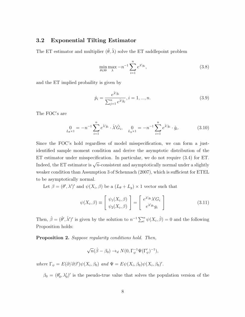
5 Main Result

Let f(Xi, β) be a vector containing the unique components of φ(Xi, β) and its deriva-

tives with respect to the components of β through order d, and φ(Xi, β)φ(Xi, β)′

and its derivatives with respect to the components of β through order d − 1. Let g

and G(j) be an element of gi and G(j)i , respectively, for j = 1, ..., d + 1. In addition,

let gk be a multiplication of any k-combination of elements of gi. For instance, if

g(Xi, θ) = (gi,1, gi,2)′, a 2 × 1 vector, then g2 = g2i,1, gi,1gi,2, or g2

i,2. G(j)k are defined

analogously. Then, f(Xi, β) contains terms of the form

α · ekτλ′gi · gk0 ·Gk1 ·G(2)k2 · · ·G(d+1)kd+1 ,

where kτ = 0, 1, 2, k0 ≤ d + 3, kj ≤ d + 2 − j, 0 ≤∑d+1

j=0 kj ≤ d + 3, and kj’s are

nonnegative integers for j = 1, ..., d+ 1 and where α denotes products of components

of β.

Assumption 1. Xi, i = 1, 2, ... are iid.

Assumption 2.

(a) Θ is compact and θ0 is an interior point of Θ; Λ(θ) is a compact set such that

λ0(θ) is an interior point of Λ(θ).

(b) For some function Cg(x), ‖g(x, θ1)− g(x, θ2)‖ < Cg(x)‖θ1 − θ2‖ for all x in the

support of X1 and all θ1, θ2 ∈ Θ; ECqgg (X1) < ∞ and E‖g(X1, θ)‖qg < ∞ for

all θ ∈ Θ for all 0 < qg <∞.

(c) For some function Cτ (x), |eλ′1g(x,θ1) − eλ′2g(x,θ2)| < Cτ (x)‖(λ′1, θ′1) − (λ′2, θ′2)‖, for

all x in the support of X1 and all (λ′1, θ′1), (λ′2, θ

′2) ∈ Λ(θ)× Θ; ECqτ

τ (X1) < ∞and Eeλ

′g(X1,θ)·qτ <∞ for all (λ′, θ′) ∈ Λ(θ)×Θ for some qτ ≥ 2.

Assumption 3.

(a) Γ0 is nonsigular.

(b) g(x, θ) is d+1 times differentiable with respect to θ on N(θ0), some neighborhood

of θ0, for all x in the support of X1, where d ≥ 1.

14

(c) There is a function CG(X1) such that ‖G(j)(X1, θ)−G(j)(X1, θ0)‖ ≤ CG(X1)‖θ−θ0‖ for all θ ∈ N(θ0) for j = 0, 1, ..., d; ECqG

G (X1) <∞ and E‖G(j)(X1, θ0)‖qG <∞ for j = 0, 1, ..., d+ 1 for all 0 < qG <∞.

Assumption 4. There exists a nonempty open subset U of Rdim(X1) with the follow-

ing properties:

(a) the distribution F of X1 has a nonzero absolutely continuous component with

respect to Lebesgue measure on Rdim(X1) with a positive density on U , and

(b) f(X1, β0) is continuously differentiable on U .

Assumption 1 is that the sample is iid, which is also assumed in Schennach (2007).

Assumption 2(a)-(b) are similar to Assumption 2(a)-(b) of Andrews (2002). Assump-

tion 2(c) is needed especially for the ETEL estimator, and is similar to but slightly

stronger than Assumption 3(4)-(6) of Schennach (2007). Assumption 3(a), (b), and

(d) are usual regularity conditions for well-defined covariance matrix and moment

function. Assumption 3(c) is similar to Assumption 3(d)-(e) of Andrews (2001), ex-

cept that I specify the form of f(Xi, β) and replace f(Xi, β) with the derivatives of

the moment function. The standard Cramer condition for Edgeworth expansion holds

if Assumption 4 holds.

The moment conditions in Assumptions 2-3 that the statements hold for all 0 <

qg, qG < ∞ are slightly stronger than necessary, but yield a simpler result. This is

also assumed in Andrews (2002) for the same reason.

Theorem 1 shows that the misspecification-robust bootstrap symmetric two-sided

t test and percentile t interval achieve asymptotic refinements over the asymptotic

test and confidence interval. This result is new, because asymptotic refinements for

the EL estimators, including the ETEL, have not been established in the existing

literature even under correct model specifications.

Recall that the asymptotic test and CI are correct up to O(n−1). Theorem 1(a)

describes the minimum requirement for asymptotic refinements of the bootstrap. This

result is comparable to Theorem 3 of Hall and Horowitz (1996), that establishes the

same magnitude of asymptotic refinements for GMM estimators. Theorem 1(b) is

that the bootstrap test and CI achieve the sharp magnitude of asymptotic refine-

ments under more stronger conditions. This result is comparable to Theorem 2(c) of

15

Andrews (2002) and Theorem 1 of Lee (2012), where the former holds under correct

model specifications and the latter is robust to model misspecifications.

The degree of asymptotic refinements varies according to qτ and d. qτ determines

the set that the moment generating function Mθ(λ) = Eeλ′gi exists. d is the number

of differentiability of the moment function, g(Xi, θ).

Theorem 1. Assume that T (χn), T (χ∗n), CIn, and CI∗n are based on the ETEL

estimator.

(a) Suppose Assumptions 1-4 hold with qτ = 32(1 + ζ) for any ζ > 0 and d = 4.

Under H0 : θr = θ0,r,

P (|T (χn)| > z∗|T |,α) = α + o(n−1) or P (θ0,r ∈ CI∗n) = 1− α + o(n−1);

(b) Suppose Assumptions 1-4 hold with all qτ <∞ and d = 6. Under H0 : θr = θ0,r,

P (|T (χn)| > z∗|T |,α) = α +O(n−2) or P (θ0,r ∈ CI∗n) = 1− α +O(n−2),

where z∗|T |,α is the 1− α quantile of the distribution of |T (χ∗n)|.

Since ET requires weaker conditions than ETEL, the above result holds for ET.

For EL, we need to assume that the moment function is bounded, (3.4). With that

assumption, an analogous result with Theorem 1 can be established. [WILL BE

ADDED]

6 Monte Carlo Experiments

6.1 An Example: Estimating the mean

Let Xi = (Yi, Zi)′ be iid sample from two independent normal distributions: Yi ∼

N(1, 1) and Zi ∼ N(1− δ, 1), where 0 ≤ δ < 1. Let

g(Xi, θ) =

(θYi − 1

θZi − 1

)

be a vector-valued function. A moment condition is Eg(Xi, θ0) = 0. In words, the

moment condition implies that Yi and Zi have the same nonzero and finite mean

16

θ−10 . The parameter δ measures a degree of misspecification. δ = 0 implies no

misspecification, that is, the two random variables have the same mean. As δ tends

to one, EZi decreases to zero and the degree of misspecification becomes larger.

The ETEL estimator is calculated by solving the equation (3.15). The estimator

does not have a closed form solution, and should be solved numerically. Nevertheless,

the probability limit of the estimator can be calculated analytically for this particular

example. By definition, λ0(θ) ≡ (λ0,1(θ), λ0,2(θ))′ is the solution to Eeλ′gigi = 0. The

pseudo-true value θ0 maximizes the criterion

lnL(θ) ≡ − lnEeλ0(θ)′(gi−Egi).

By solving the equations, we have

(λ0,1(θ), λ0,2(θ)) =

(1− θ0

θ20

,1− (1− δ)θ0

θ20

), θ0 =

2

2− δ.

Note that θ0 = 1 when δ = 0, i.e., the model is correctly specified. In addition, the

corresponding λ0,1 and λ0,2 become zeros when δ = 0.

6.2 Confidence Intervals

In this section, I describe asymptotic and bootstrap CI’s based on the ET and ETEL

estimators. For brevity, let Lθ = 1.

6.2.1 Conventional CI based on the EL estimator

I first consider the EL estimator, θEL. According to its asymptotic theory, under

correct model specifications, we have

√n(θEL − θ0)→d N(0, (G′0Ω−1

0 G0)−1),

where Ω0 = Egi(θ0)gi(θ0)′ and θ0 is the true value that satisfies Egi(θ0) = 0. The

asymptotic covariance matrix can be estimated by ΣC = (G′nΩ−1n Gn)−1, where Gn =

n−1∑n

i=1 Gi and Ωn = n−1∑n

i=1 gig′i. Then, the 100(1− α)% asymptotic CI for θ0 is

given by

Asymp.EL:

(θEL ± zα/2

√ΣC/n

).

17

This conventional CI yields correct coverage probability 1 − α only if the model is

correctly specified, because the covariance estimator ΣC is not consistent for the true

covariance matrix under misspecification.

I also consider the bootstrap CI based on the EL estimator using the efficient

bootstrapping suggested by Brown and Newey (2002), that utilizes the EL probability

in resampling. Although their paper is on constructing the bootstrap CI based on the

GMM estimator, not the EL estimator, it is natural to apply the procedure to the

EL estimator. The key procedure is to use the EL-estimated distribution function,

FEL(z) =∑n

i=1 1(Xi ≤ z)pi, where pi = n−1(1 − λ′ELgi)−1, in place of the edf, Fn.

The bootstrap procedure is as follows: (i) For a given sample, calculate (λ′EL, θ′EL)′

and pi’s, (ii) Draw the bootstrap sample with replacement from FEL, (iii) Calculate

T ∗EL,n ≡ (θ∗EL − θEL)/√

Σ∗C/n, where Σ∗C = (G∗′n Ω∗−1

n G∗n)−1, G∗n = n−1∑n

i=1 G∗i and

Ω∗n = n−1∑n

i=1 g∗i g∗′i , (iv) repeat this B times and get the distribution of |T ∗EL,n|,

(iv) Find the 1 − α quantile z∗|TEL|,α of the distribution of |T ∗EL,n| and construct the

symmetric percentile t interval,

BN-Boot.EL:

(θEL ± z∗|TEL|,α

√ΣC/n

).

This CI would yield correct coverage probability 1− α only if the model is correctly

specified. Under misspecifications, this CI would not work because (i) ΣC is inconsis-

tent for the true covariance matrix under misspecification and (ii) FEL is inconsistent

for the true distribution F . Moreover, in the simulation described in the following

section, some of the EL probabilities had negative values under misspecifications,

making the EL weighted resampling hard to be implemented.

6.2.2 Misspecification-Robust CI based on the EL estimator

Based on the same EL estimator, we can construct misspecification-robust asymptotic

and bootstrap CI’s.

MR-Asymp.EL:

(θEL ± zα/2

√ΣEL/n

),

MR-Boot.EL:

(θEL ± z∗|T |,α

√ΣEL/n

),

18

where all the quantities are defined in the previous sections. These CI’s are robust

to misspecification. Moreover, the bootstrap symmetric percentile t interval MR-

Boot.EL achieves asymptotic refinements over the asymptotic CI MR-Asymp.EL.

6.2.3 Misspecification-Robust CI based on the ETEL estimator

Finally, I consider the asymptotic and the bootstrap CI’s based on the ETEL esti-

mator θ:

MR-Asymp.ETEL:

(θ ± zα/2

√Σ/n

),

MR-Boot.ETEL:

(θ ± z∗|T |,α

√Σ/n

),

where all the quantities are defined in the previous sections. These CI’s are robust

to misspecification. Moreover, the bootstrap symmetric percentile t interval MR-

Boot.ETEL achieves asymptotic refinements over the asymptotic CI MR-Asymp.ETEL,

according to Theorem 1.

6.3 Simulation Result

Table 1 presents the coverage probabilities of 90% and 95% CI’s for the (pseudo-

)true value θ0 based on the ETEL or EL estimator under model misspecifications.

δ denotes a degree of misspecification. As δ gets larger, the model becomes more

misspecified. δ = 0 implies that the model is correctly specified. Both the numbers of

Monte Carlo repetition (r) and the bootstrap repetition (B) are 1,000. The (actual)

coverage probabilities are given by

Coverage Probability of CI =

∑r 1(θ0 ∈ CI)

r,

where CI is either Asymp.EL, MR-Asymp.ETEL, or MR-Boot.ETEL. Since the nom-

inal coverage probabilities are given by 90% and 95%, CI’s that yield actual coverage

probabilities close to 0.90 and 0.95 are favorable.

Consider the case δ = 0. MR-Boot.ETEL performs better than Asymp.ETEL,

especially when n = 25. This confirms Theorem 1. Although Theorem 1 does not

establish asymptotic refinements of BN-Boot.EL, the simulation result shows that

BN-Boot.EL performs better than the asymptotic CI based on the EL estimator

19

Degree of n = 25 n = 50

Misspecification CI’s 90% 95% 90% 95%

Asymp.EL 0.877 0.919 0.896 0.949δ = 0 BN-Boot.EL 0.899 0.954 0.916 0.962

(none) MR-Asymp.ETEL 0.880 0.925 0.903 0.950MR-Boot.ETEL 0.904 0.962 0.914 0.959

over-ID test, 1% level1.5% 1.0%

(Rejection Prob.)

Asymp.EL 0.834 0.886 0.834 0.897δ = 0.5 BN-Boot.EL 0.858 0.909 0.831 0.902

(moderate) MR-Asymp.ETEL 0.876 0.912 0.886 0.932MR-Boot.ETEL 0.911 0.945 0.909 0.956


(Rejection Prob.)

Asymp.EL 0.748 0.812 0.719 0.789δ = 0.75 BN-Boot.EL 0.717 0.769 0.574 0.642

(large) MR-Asymp.ETEL 0.820 0.850 0.872 0.915MR-Boot.ETEL 0.866 0.911 0.900 0.938


(Rejection Prob.)

Table 1: Coverage Probabilities of 90% and 95% Confidence Intervals for θ0 underModel Misspecifications

Asymp.EL when n = 25. Asymptotic refinements of the bootstrap CI’s become less

clear when n = 50, for both MR-Boot.ETEL and BN-Boot.EL. If we use a non-

Normal distribution for the data-generating process, then asymptotic refinements of

the bootstrap would be clearer than those shown in Table 1.

When the model is misspecified, δ = 0.5 or δ = 0.75, the CI’s based on the

conventional EL estimator, Asymp.EL and BN-Boot.EL, seem to fail to yield cor-

rect coverage probabilities asymptotically. In addition, BN-Boot.EL loses asymptotic

refinements over Asymp.EL. In contrast, the CI’s based on the ETEL estimator,

MR-Asymp.ETEL and MR-Boot.ETEL, are robust to misspecification as expected.

MR-Boot.ETEL does not lose the ability of asymptotic refinements even if the model

is misspecified. This supports Theorem 1.

20

One might argue that any misspecification in the model could be detected by

using the overidentifying restrictions test. I emphasize that the test does not always

reject the misspecified model and in fact, the rejection probability is quite low in

small sample. The rejection probabilities of the EL overidentifying restrictions test

are reported in Table 1: over-ID test, 1% level (Rejection Prob.). The null hypothesis

of correct model specifications is rejected at 1% level. For instance, when n = 25 and

δ = 0.5, the probability that the overidentifying restrictions test correctly rejects the

misspecified model is 22.2%. When n = 25 and δ = 0.75, the chance of rejecting the

misspecified model is 56.8%, even if there is a large misspecification. If one proceeds

with the misspecified model using the conventional EL estimator, then inferences and

CI’s would be invalid.

References

Allen, J., A. W. Gregory, and K. Shimotsu (2011): “Empirical Likelihood Block Bootstrap-

ping,” Journal of Econometrics 161, 110-121.

Andrews, D. W. W. (2001): “Higher-Order Improvements of a Computationally Attractive k-

step Boostrap for Extremum Estimators,” Cowles Foundation Discussion Paper No. 1269,

Yale University. Available at http://cowles.econ.yale.edu.

Andrews, D. W. W. (2002): “Higher-Order Improvements of a Computationally Attractive

k-step Boostrap for Extremum Estimators,”Econometrica, 70, 119-162.

Beran, R. (1988): “Prepivoting test statistics: a bootstrap view of asymptotic refinements,”

Journal of the American Statistical Association, 83, 687-697.

Bhattacharya, R. N. (1987): “Some Aspects of Edgeworth Expansions in Statistics and Prob-

ability,” in New Perspectives in Theoretical and Applied Statistics, ed. by M. L. Puri, J.P.

Vilaploma, and W. Wertz. New York: Wiley, 157-170.

Bhattacharya, R. N. and J. K. Ghosh (1978): “On the Validity of the Formal Edgeworth

Expansion,” Annals of Statistics, 6, 434-451.

Brown, B.W. and W.K. Newey (2002): “Generalized Method of Moments, Efficient Bootstrap-

ping, and Improved Inference,” Journal of Business and Economic Statistics 20, 507-517.

Canay, I.A. (2010): “EL Inference for Partially Identified Models: Large Deviations Optimality

and Bootstrap Validity,” Journal of Econometrics 156, 408-425.

Chen, X., H. Hong and M. Shum (2007): “Nonparametric likelihood ratio model selection tests

between parametric likelihood and moment condition models,” Journal of Econometrics 141,

109-140.

21

http://cowles.econ.yale.edu

Efron, B. and R. Tibshirani (1993): An introduction to the bootstrap, London: Chapman and

Hall.

Golcalves, S. and H. White (2004): Maximum Likelihood and the Bootstrap for Nonlinear

Dynamic Models, Journal of Econometrics 119, 199-219.

Gotze, F. and C. Hipp (1983): “Asymptotic Expansions for Sums of Weakly Dependent Random

Vectors,” Wahrscheinlichkeitstheorie verw. Gebiete, 64, 211-239.

Hahn, J. (1996): “A Note on Bootstrapping Generalized Method of Moments Estimators,” Econo-

metric Theory 12, 187-197.

Hall, P. (1988): “On Symmetric Bootstrap Confidence Intervals,” Journal of the Royal Statistical

Society, Series B, 50, 35-45.

Hall, P. (1992): The bootstrap and Edgeworth expansion, New York: Springer-Verlag.

Hall, P. and J. L. Horowitz (1996): “Bootstrap Critical Values for Tests Based on Generalized-

Method-of-Moments Estimators,” Econometrica 64, 891-916.

Hansen, B. E. (2011): Econometrics, manuscript. Department of Economics, University of

Wisconsin-Madison.

Hansen, L. P. (1982): “Large Sample Properties of Generalized Method of Moments Estimators,”

Econometrica 50, 1029-1054.

Hansen, L. P., J. Heaton, and A. Yaron (1996): “Finite-Sample Properties of Some Alter-

native GMM Estimators,” Journal of Business and Economic Statistics 14, 262-280.

Horowitz, J. L. (2001): “The Bootstrap,” in James J. Heckman and E. Leamer eds., Handbook

of Econometrics, Vol. 5, New York: Elsevier Science.

Horowitz, J. L. (2003): “Bootstrap methods for Markov processes,” Econometrica 71, 1049-1082.

Imbens, G. W. (1997): “One-Step Estimators for Over-Identified Generalized Method of Moments

Models,” The Review of Economic Studies 64, 359-383.

Imbens, G. W., R. H. Spady, and P. Johnson (1998): “Information Theoretic Approaches to

Inference in Moment Condition Models,” Econometrica 66, 333-357.

Inoue, A. and M. Shintani (2006): “Bootstrapping GMM Estimators for Time Series,” Journal

of Econometrics 133, 531-555.

Kitamura, Y. and M. Stutzer (1997): “An Information-Theoretic Alternative to Generalized

Method of Moment Estimation,” Econometrica 65, 861-874.

Kitamura, Y., T. Otsu, and K. Evdokimov (2013): “Robustness, Infinitesimal Neighbor-

hoods, and Moment Restictions,” forthcoming in Econometrica.

Lee, S. J. (2012): “Asymptotic Refinements of a Misspecification-Robust Bootstrap for General-

ized Method of Moments Estimators,” Working paper, University of New South Wales.

22

Newey, W. K. and D. McFadden (1994): “Large Sample Estimation and Hypothesis Testing,”

in R. Engle and D. McFadden eds., Handbook of Econometrics, Vol. 4, North-Holland.

Newey, W. K. and R. J. Smith (2004): “Higher-Order Properties of GMM and Generalized

Empirical Likelihood Estimators,” Econometrica 72, 219-255.

Owen, A. B. (1988): “Empirical Likelihood Ratio Confidence Intervals for a Single Functional,”

Biometrika 75, 237-249.

Owen, A. B. (1990): “Empirical Likelihood Ratio Confidence Regions,” Annals of Statistics 18,

90-120.

Qin, J. and J. Lawless (1988): “Empirical Likelihood and General Estimating Equations,”

Annals of Statistics 22, 300-325.

Schennach, S. M. (2007): “Point Estimation with Exponentially Tilted Empirical Likelihood,”

Annals of Statistics 35, 634-672.

White, H. (1982): “Maximum Likelihood Estimation of Misspecified Models,” Econometrica 50,

1-25.

Windmeijer, F. (2005): “A Finite Sample Correction for the Variance of Linear Efficient Two-step

GMM Estimators,” Journal of Econometrics 126, 25-51.

A Appendix: Lemmas and Proofs

A.1 Lemmas

Lemma 1 is a nonparametric iid bootstrap version of Lemma 1 of Andrews (2002).

Lemma 1. Suppose Assumption 1 holds.

(a) Let h(·) be a matrix-valued function that satisfies Eh(Xi) = 0 and E‖h(Xi)‖p < ∞ for p ≥ 2

and p > 2a/(1− 2c) for some c ∈ [0, 1/2) and a ≥ 0. Then, for all ε > 0,

limn→∞

naP

(∥∥∥∥∥n−1n∑i=1

h(Xi)

∥∥∥∥∥ > n−cε

)= 0.

(b) Let h(·) be a matrix-valued function that satisfies E‖h(Xi)‖p < ∞ for p ≥ 2 and p > 2a for

some a ≥ 0. Then, there exists a constant K <∞ such that

limn→∞

naP

(∥∥∥∥∥n−1n∑i=1

h(Xi)

∥∥∥∥∥ > K

)= 0.

In the following Lemmas, we assume that a = 1 or 2, because these values are only required

in the proofs of the Theorems. This simplifies the conditions for the Lemmas. See Lee (2011c) for

similar results for any a ≥ 0.

23

Lemma 2. Suppose Assumptions 1-3 hold with qτ > 2a. Then, for all ε > 0,

(a) limn→∞

naP

(supθ∈Θ

∥∥∥∥∥n−1n∑i=1

(gi(θ)− Egi(θ))

∥∥∥∥∥ > ε

)= 0,

(b) limn→∞

naP

(supθ∈Θ

∣∣∣∣∣n−1n∑i=1

(eλ(θ)′gi(θ) − Eeλ0(θ)′gi(θ)

)∣∣∣∣∣ > ε

)= 0,

(c) limn→∞

naP

(supθ∈Θ

∥∥∥λ(θ)− λ0(θ)∥∥∥ > ε

)= 0.

Let τ0(θ) ≡ Eeλ0(θ)′gi(θ) and κ0(θ) ≡ −(Eeλ0(θ)′gi(θ)gi(θ)gi(θ)′)−1τ0(θ)Egi(θ). Analogous to

the definition of Λ(θ), define T (θ) and K(θ) be compact sets such that τ0(θ) ∈ int(T (θ)) and

κ0(θ) ∈ int(K(θ)). For β ≡ (τ, κ′, λ′, θ′)′, define a compact set B ≡ T (θ)×K(θ)× Λ(θ)×Θ.

Lemma 3. Suppose Assumptions 1-3 hold with qτ > 2a(1 + ζ) for any ζ > 0. Then, for all ε > 0,

limn→∞

naP(‖β − β0‖ > ε

)= 0,

where β0 = (τ0, κ′0, λ′0, θ′0)′ and β = (τ , κ′, λ′, θ′)′.

Lemma 4. Suppose Assumptions 1-3 hold with qτ > 2a1−2c (1 + ζ) for any ζ > 0. Then, for all

c ∈ [0, 1/2) and ε > 0,

limn→∞

naP(‖β − β0‖ > n−c

)= 0,

where β0 = (τ0, κ′0, λ′0, θ′0)′ and β = (τ , κ′, λ′, θ′)′.

Lemma 5 is identical to Andrews (2002). We restate it for convenience.

Lemma 5. (a) Let An : n ≥ 1 be a sequence of LA × 1 random vectors with either (i) uniformly

bounded densities over n > 1 or (ii) an Edgeworth expansion with coefficients of order O(1)

and remainder of order o(n−a) for some a ≥ 0 (i.e., for some polynomials πi(δ) in δ =

∂/∂z whose coefficients are O(1) for i = 1, ..., 2a, limn→∞ na supz∈RLA |P (An ≤ z) − [1 +∑2ai=1 n

−i/2πi(∂/∂z)]ΦΣn(z)| = 0, where ΦΣn(z) is the distribution function of a N(0,Σn)

random variable and the eigenvalues of Σn are bounded away from 0 and ∞ for n ≥ 1). Let

ξn : n ≥ 1 be a sequence of LA × 1 random vectors with P (‖ξn‖ > ϑn) = o(n−a) for some

constants ϑn = o(n−a) and some a ≥ 0. Then,

limn→∞

supz∈RLA

na |P (An + ξn ≤ z)− P (An ≤ z)| = 0.

(b) Let A∗n : n ≥ 1 be a sequence of LA×1 bootstrap random vectors that possesses an Edgeworth

expansion with coefficients of order O(1) and remainder of order o(n−a) that holds except if

χn : n ≥ 1 are in a sequence of sets with probability o(n−a) for some a ≥ 0. (That is, for all

ε > 0, limn→∞ naP (na supz∈RLA |P∗(A∗n ≤ z) − [1 +

∑2ai=1 n

−i/2π∗i (∂/∂z)]ΦΣ∗n(z)| > ε) = 0,

24

where π∗i (δ) are polynomials in δ = ∂/∂z whose coefficients, C∗n, satisfy: for all ρ > 0, there

exists Kρ < ∞ such that limn→∞ naP (P ∗(|C∗n| > Kρ) > ρ) = 0 for all i = 1, ..., 2a, ΦΣ∗n(z)

is the distribution function of a N(0,Σ∗n) random variable conditional on Σ∗n and Σ∗n is a

possibly random matrix whose eigenvalues are bounded away from 0 and ∞ with probability

1 − o(n−a) ad n → ∞.) Let ξ∗n : n ≥ 1 be a sequence of LA × 1 random vectors with

limn→∞ naP (P ∗(‖ξ∗n‖ > ϑn) > n−a) = 0 for some constants ϑn = o(n−a). Then,

limn→∞

naP

(sup

z∈RLA|P ∗(A∗n + ξ∗n ≤ z)− P ∗(A∗n ≤ z)| > n−a

)= 0.

Let P ∗ be the probability distribution of the bootstrap sample conditional on the original sample.

Let E∗ denote expectation with respect to the distribution of the bootstrap sample conditional on

the original sample. Since we consider iid sample and nonparametric iid bootstrap, E∗ is taken

over the original sample with respect to the empirical distribution function. For example, E∗X∗i =

n−1∑ni=1Xi.

Lemma 6 is a nonparametric iid bootstrap version of Lemma 6 of Andrews (2002).

Lemma 6. Suppose Assumption 1 holds. Let h(·) be a matrix-valued function that satisfies Eh(Xi) =

0 and E‖h(Xi)‖p <∞ for p ≥ 2 and p > 4a/(1− 2c) for some c ∈ [0, 1/2) and a ≥ 0. Then,

(a) limn→∞

naP

(P ∗

(∥∥∥∥∥n−1n∑i=1

h(X∗i )− E∗h(X∗i )

∥∥∥∥∥ > n−c

)> n−a

)= 0,

(b) limn→∞

naP

(P ∗

(∥∥∥∥∥n−1n∑i=1

E∗h(X∗i )

∥∥∥∥∥ > n−c

)> n−a

)= 0,

(c) limn→∞

naP

(P ∗

(∥∥∥∥∥n−1n∑i=1

h(X∗i )

∥∥∥∥∥ > n−c

)> n−a

)= 0,

(d) limn→∞

naP

(P ∗

(∥∥∥∥∥n−1n∑i=1

E∗h(X∗i )

∥∥∥∥∥ > K

)> n−a

)= 0 and

limn→∞

naP

(P ∗

(∥∥∥∥∥n−1n∑i=1

h(X∗i )

∥∥∥∥∥ > K

)> n−a

)= 0,

for some K <∞, even if Eh(Xi) 6= 0 and p only satisfies p ≥ 2 and p > 4a in part (d).

Lemma 7. Suppose Assumptions 1-3 hold with qτ > 4a. Then, for all ε > 0,

(a) limn→∞

naP

(P ∗

(supθ∈Θ

∥∥∥∥∥n−1n∑i=1

(g∗i (θ)− E∗g∗i (θ))

∥∥∥∥∥ > ε

)> n−a

)= 0,

(b) limn→∞

naP

(P ∗

(supθ∈Θ

∣∣∣∣∣n−1n∑i=1

(eλ∗(θ)′g∗i (θ) − eλ(θ)′gi(θ)

)∣∣∣∣∣ > ε

)> n−a

)= 0,

(c) limn→∞

naP

(P ∗(

supθ∈Θ

∥∥∥λ∗(θ)− λ(θ)∥∥∥ > ε

)> n−a

)= 0.

25

Lemma 8. Suppose Assumptions 1-3 hold with qτ > 4a(1 + ζ) for any ζ > 0. Then, for all ε > 0,

limn→∞

naP(P ∗(‖β∗ − β‖ > ε

)> n−a

)= 0,

where β∗ = (τ∗, κ∗′, λ∗

′, θ∗′)′ and β = (τ , κ′, λ′, θ′)′.

Lemma 9. Suppose Assumptions 1-3 hold with qτ > 4a1−2c (1 + ζ) for any ζ > 0. Then, for all

c ∈ [0, 1/2) and ε > 0,

limn→∞

naP(P ∗(‖β∗ − β‖ > n−c

)> n−a

)= 0,

where β∗ = (τ∗, κ∗′, λ∗

′, θ∗′)′ and β = (τ , κ′, λ′, θ′)′.

Lemma 10. (a) Suppose Assumptions 1-3 hold with qτ > 4a(1 + ζ) for any ζ > 0. Then, for all

β ∈ N(β0), some K <∞, and some C(Xi) that satisfies limn→∞ naP (‖n−1∑ni=1 C(Xi)‖ > K) = 0,

‖f(Xi, β)− f(Xi, β0)‖ ≤ C(Xi)‖β − β0‖.

(b) Suppose Assumptions 1-3 hold with qτ > 8a(1+ζ) for some ζ > 0. Then, for all β ∈ N(β0), some

K <∞, and some C∗(X∗i ) that satisfies limn→∞ naP (P ∗(‖n−1∑ni=1 C

∗(X∗i )‖ > K) > n−a) = 0,

‖f(X∗i , β)− f(X∗i , β0)‖ ≤ C∗(X∗i )‖β − β0‖.

We now introduce some additional notation. Let Sn be the vector containing the unique compo-

nents of n−1∑ni=1 f(Xi, β0) on the support of Xi, and S = ESn. Similarly, let S∗n denote the vector

containing the unique components of n−1∑ni=1 f(X∗i , β) on the support of Xi, and S∗ = E∗S∗n.

Lemma 11. (a) Suppose Assumptions 1-3 hold with qτ > 4a(1 + ζ) for any ζ > 0. Then, for all

ε > 0,

limn→∞

naP (‖Sn − S‖ > ε) = 0.

(b) Suppose Assumptions 1-3 hold with qτ > 8a(1 + ζ) for any ζ > 0. Then, for all ε > 0,

limn→∞

naP(P ∗ (‖S∗n − S∗‖ > ε) > n−a

)= 0.

Lemma 12. Let ∆n and ∆∗n denote√n(θ− θ0) and

√n(θ∗− θ), or Tn and T ∗n . For each definition

of ∆n and ∆∗n, there is an infinitely differentiable function A(·) with A(S) = 0 and A(S∗) = 0 such

that the following results hold.

26

(a) Suppose Assumptions 1-4 hold with qτ > max

2add−2a−1 , 4a

·(1+ζ) for any ζ > 0, and d ≥ 2a+2,

where 2a is some positive integer. Then,

limn→∞

supzna|P (∆n ≤ z)− P (

√nA(Sn) ≤ z)| = 0.

(b) Suppose Assumptions 1-4 hold with qτ > max

4add−2a−1 , 8a

·(1+ζ) for any ζ > 0, and d ≥ 2a+2,

where 2a is some positive integer. Then,

limn→∞

naP

(supz|P ∗(∆∗n ≤ z)− P ∗(

√nA(S∗n) ≤ z)| > n−a

)= 0.

We define the components of the Edgeworth expansions of the test statistic Tn and its bootstrap

analog T ∗n . Let Ψn =√n(Sn − S) and Ψ∗n =

√n(S∗n − S∗). Let Ψn,j and Ψ∗n,j denote the jth

elements of Ψn and Ψ∗n respectively. Let νn,a and ν∗n,a denote vectors of moments of the form

nα(m)EΠmµ=1Ψn,jµ and nα(m)E∗Πm

µ=1Ψ∗n,jµ , respectively, where 2 ≤ m ≤ 2a + 2, α(m) = 0 if m is

even, and α(m) = 1/2 if m is odd. Let νa = limn→∞ νn,a. The existence of the limit is proved in

Lemma 13.

Let πi(δ, νa) be a polynomial in δ = ∂/∂z whose coefficients are polynomials in the elements of

νa and for which πi(δ, νa)Φ(z) is an even function of z when i is odd and is an odd function of z

when i is even for i = 1, ..., 2a, where 2a is an integer. The Edgeworth expansions of Tn and T ∗ndepend on πi(δ, νa) and πi(δ, ν

∗n,a), respectively.

Lemma 13. (a) Suppose Assumptions 1-3 hold with qτ ≥ 4(a+ 1)(1 + ζ) for any ζ > 0. Then, νn,a

and νa ≡ limn→∞ νn,a exist.

(b) Suppose Assumptions 1-3 hold with qτ >16a(a+1)

1−2γ (1 + ζ) for any ζ > 0 and γ ∈ [0, 1/2). Then,

limn→∞

naP(‖ν∗n,a − νa‖ > n−γ

)= 0.

Lemma 14. (a) Suppose Assumptions 1-4 hold with qτ ≥ 4(a + 1)(1 + ζ) and qτ >2ad

d−2a−1 (1 + ζ)

for any ζ > 0, and d ≥ 2a+ 2, where 2a is some positive integer. Then,

limn→∞

na supz∈R

∣∣∣∣∣P (Tn ≤ z)−

[1 +

2a∑i=1

n−i/2πi(δ, νa)

]Φ(z)

∣∣∣∣∣ = 0.

(b) Suppose Assumptions 1-4 hold with qτ > max

4add−2a−1 , 16a(a+ 1)

· (1 + ζ) for any ζ > 0, and

d ≥ 2a+ 2, where 2a is some positive integer. Then,

limn→∞

naP

(supz∈R

∣∣∣∣∣P ∗(T ∗n ≤ z)−[

1 +

2a∑i=1

n−i/2πi(δ, ν∗n,a)

]Φ(z)

∣∣∣∣∣ > n−a

)= 0.

27

A.2 Proof of Proposition 1

Proof. A PROOF WILL BE PROVIDED.

A.3 Proof of Theorem 1

Proof of (a). Let a = 1. We apply Lemma 13 with γ = 0 and Lemma 14. Letting d = 4 and

qτ = 32(1 + ζ) for all ζ > 0 satisfies the required condition. The proof mimics that of Theorem 2

of Andrews (2001). By the evenness of πi(δ, ν1)Φ(z) and πi(δ, ν∗n,1)Φ(z), for any ε > 0, Lemma 14

yields

supz∈R

∣∣P (|Tn| ≤ z)−[1 + n−1π2(δ, ν1)

](Φ(z)− Φ(−z))

∣∣ = o(n−1),

P

(supz∈R

∣∣P ∗(|T ∗n | ≤ z)− [1 + n−1π2(δ, ν∗n,1)]

(Φ(z)− Φ(−z))∣∣ > n−1ε

)= o(n−1).

By Lemma 13 with γ = 0,

P

(supz∈R|P (|Tn| ≤ z)− P ∗(|T ∗n | ≤ z)| > n−1ε

)≤ P

(n−1|π2(δ, ν1)− π2(δ, ν∗n,1)| > n−1ε

)+ o(n−1) = o(n−1). (A.1)

Then by (A.1),

P(∣∣∣P ∗(|T ∗n | ≤ z∗|T |,α)− P (|Tn| ≤ z∗|T |,α)

∣∣∣ > n−1ε)

= P(|1− α− F|T |(z∗|T |,α)| > n−1ε

)= o(n−1), (A.2)

where F|T |(·) denote the distribution function of |Tn|. Using (A.2), we have

P (|Tn > z∗|T |,α)

= P(F|T |(|Tn|) > F|T |(z

∗|T |,α), |1− α− F|T |(z∗|T |,α)| ≤ n−1ε

)+P

(F|T |(|Tn|) > F|T |(z

∗|T |,α), |1− α− F|T |(z∗|T |,α)| > n−1ε

)≤ P (F|T |(|Tn|) > 1− α− n−1ε) + P (|1− α− F|T |(z∗|T |,α)| > n−1ε)

≤ α+ n−1ε+ o(n−1), (A.3)

and similarly,

P (|Tn > z∗|T |,α) ≥ P (F|T |(|Tn|) > 1− α− n−1ε) ≥ α− n−1ε. (A.4)

Combining (A.3) and (A.4) establishes the present Theorem (a).

Proof of (b). The proof is the same with that of Theorem 2(c) of Andrews (2002) with his Lemmas

28

13 and 16 replaced by our Lemmas 12 and 14. The proof relies on the argument of Hall (1988,

1992)’s methods developed for “smooth functions of sample averages,” for iid data. Q.E.D.

A.4 Proofs of Lemmas

A.4.1 Proof of Lemma 1

Proof. Assumption 1 of Andrews (2002) is satisfied if Assumption 1 holds. Then, Lemma 1 of

Andrews (2002) holds. Q.E.D.


Proof. The present Lemma (a) is proved by the proof of Lemma 2 of Lee (2011), that also follows

the proof of Lemma 2 of Hall and Horowitz (1996). We apply Lemma 1 with c = 0 and p = qg using

Assumption 2(b).

Proving the present Lemma (b) and (c) involves several steps. First, we need to show2 that

limn→∞

naP

(sup

(λ′,θ′)′∈Λ(θ)×Θ

∥∥∥∥∥n−1n∑i=1

eλ′gi(θ) − Eeλ

′gi(θ)

∥∥∥∥∥ > ε

)= 0. (A.5)

We apply similar arguments to the proof of Lemma 2 of Lee (2011). Then, Lemma 1 with c = 0 and

p = qτ gives the result by Assumption 2(c).

Next, we show

limn→∞

naP

(supθ∈Θ

∥∥λ(θ)− λ0(θ)∥∥ > ε

)= 0, (A.6)

where λ(θ) = arg minλ∈Λ(θ) n−1∑ni=1 e

λ′gi(θ). We show (A.6) by using the arguments in the proof

of Theorem 10 of Schennach (2007). For a given ε > 0, let

η = infθ∈Θ

infλ∈Λ(θ)

‖λ−λ0(θ)‖>ε

(Eeλ′gi(θ) − Eeλ0(θ)′gi(θ)),

which is positive by the strict convexity of Eeλ′gi(θ) in λ, λ0(θ) ≡ arg minλEe

λ′gi(θ), and the fact

that Θ is compact. By the definition of η,

P

(supθ∈Θ

(Eeλ(θ)′gi(θ) − Eeλ0(θ)′gi(θ)

)≤ η

)≤ P

(supθ∈Θ‖λ(θ)− λ0(θ)‖ ≤ ε

). (A.7)

2One may write Mθ(θ) ≡ Eeλ′gi(θ) and Mθ(θ) ≡ n−1

∑ni=1 e

λ′gi(θ) to emphasize that Eeλ′gi(θ)

and n−1∑ni=1 e

λ′gi(θ) are functions of λ and θ, and can be interpreted as the population and samplemoment generating functions, as in Schennach (2007). In the proof, however, I do not use thesenotations.

29

Since n−1∑ni=1 e

λ(θ)′gi(θ) − n−1∑ni=1 e

λ0(θ)′gi(θ) < 0,

supθ∈Θ


)≤ sup

θ∈Θ

(Eeλ(θ)′gi(θ) − n−1

n∑i=1

eλ(θ)′gi(θ)

)+ supθ∈Θ

(n−1

n∑i=1

eλ(θ)′gi(θ) − n−1n∑i=1

eλ0(θ)′gi(θ)

)

+ supθ∈Θ

(n−1

n∑i=1

eλ0(θ)′gi(θ) − Eeλ0(θ)′gi(θ)

)

≤ 2 sup(λ′,θ′)′∈Λ(θ)×Θ

∣∣∣∣∣n−1n∑i=1


′gi(θ)

∣∣∣∣∣ .Thus, we have

naP

(supθ∈Θ


)≤ η

)≥ naP

(sup

(λ′,θ′)′∈Λ(θ)×Θ

∣∣∣∣∣n−1n∑i=1


′gi(θ)

∣∣∣∣∣ ≤ η/2)→ 1,

by (A.5). Using this result, (A.7) implies (A.6). However, λ(θ) is the minimizer on Λ(θ). To get

the present Lemma (c) for λ(θ) = arg minλ∈Lg n−1∑ni=1 e

λ′gi(θ), we use the argument similar to the

proof of Theorem 2.7 of Newey and McFadden (1994). By using the convexity of n−1∑ni=1 e

λ′gi(θ)

in λ for any θ, λ(θ) = λ(θ) in the event that λ(θ) ∈ int(Λ(θ)), where int(Λ(θ)) is the interior of Λ(θ).

Take a closed neighborhood Nδ(λ0(θ)) of radius δ around λ0(θ) such that Nδ(λ0(θ)) ⊂ int(Λ(θ)).

Then, whenever λ(θ) ∈ int(Λ(θ)), ‖λ(θ)− λ0(θ)‖ ≤ δ for all θ ∈ Θ. Thus,

P

(supθ∈Θ

∥∥∥λ(θ)− λ0(θ)∥∥∥ > ε

)= P

(supθ∈Θ

∥∥∥λ(θ)− λ0(θ)∥∥∥ > ε, sup

θ∈Θ

∥∥λ(θ)− λ0(θ)∥∥ ≤ δ)

+P

(supθ∈Θ

∥∥∥λ(θ)− λ0(θ)∥∥∥ > ε, sup

θ∈Θ

∥∥λ(θ)− λ0(θ)∥∥ > δ

)≤ P

(supθ∈Θ

∥∥λ(θ)− λ0(θ)∥∥ > ε

)+ P

(supθ∈Θ

∥∥λ(θ)− λ0(θ)∥∥ > δ

)= o(n−a),

by (A.6). This proves the present Lemma (c).

The present Lemma (b) can be shown as follows. By the triangle inequality,∣∣∣∣∣n−1n∑i=1

eλ(θ)′gi(θ) − Eeλ0(θ)′gi(θ)

∣∣∣∣∣≤

∣∣∣∣∣n−1n∑i=1


eλ0(θ)′gi(θ)

∣∣∣∣∣+

∣∣∣∣∣n−1n∑i=1


∣∣∣∣∣ .

30

Combining the following results gives the desired result.

limn→∞

naP

(supθ∈Θ

∣∣∣∣∣n−1n∑i=1


eλ0(θ)′gi(θ)

∣∣∣∣∣ > ε

)= 0, (A.8)

limn→∞

naP

(supθ∈Θ

∣∣∣∣∣n−1n∑i=1


∣∣∣∣∣ > ε

)= 0. (A.9)

Since λ0(θ) ∈ int(Λ(θ)), (A.9) follows from (A.5). To show (A.8), we apply the triangle inequality

and use the fact that λ(θ) = λ(θ) in the event that λ(θ) ∈ int(Λ(θ)):

P

(supθ∈Θ

∣∣∣∣∣n−1n∑i=1


eλ0(θ)′gi(θ)

∣∣∣∣∣ > ε

)

= P

(supθ∈Θ

∣∣∣∣∣n−1n∑i=1

(eλ(θ)′gi(θ) − eλ0(θ)′gi(θ)

)∣∣∣∣∣ > ε, supθ∈Θ

∥∥λ(θ)− λ0(θ)∥∥ ≤ δ)

+P

(supθ∈Θ

∣∣∣∣∣n−1n∑i=1


)∣∣∣∣∣ > ε, supθ∈Θ

∥∥λ(θ)− λ0(θ)∥∥ > δ

)

≤ P

(supθ∈Θ

∣∣∣∣∣n−1n∑i=1


)∣∣∣∣∣ > ε

)+ P

(supθ∈Θ

∥∥λ(θ)− λ0(θ)∥∥ > δ

)

≤ P

(supθ∈Θ

∥∥λ(θ)− λ0(θ)∥∥n−1

n∑i=1

Cτ (Xi) > ε

)+ o(n−a) = o(n−a),

by applying Lemma 1(b) with h(Xi) = Cτ (Xi) and p = qτ and using the result (A.6). Q.E.D.


Proof. First, we show

limn→∞

naP

(supθ∈Θ| ln L(θ)− lnL(θ)| > ε

)= 0. (A.10)

Since

ln L(θ) = − ln

(n−1

n∑i=1

eλ(θ)′gi(θ)

)+ λ(θ)′gn(θ), and

lnL(θ) = − ln(Eeλ0(θ)′gi(θ)

)+ λ0(θ)′Egi(θ),

(A.10) follows from

limn→∞

naP

(supθ∈Θ|n−1

n∑i=1

eλ(θ)′gi(θ) − Eeλ0(θ)′gi(θ)| > ε

)= 0,

limn→∞

naP

(supθ∈Θ|λ(θ)′gn(θ)− λ0(θ)′Egi(θ)| > ε

)= 0.

31

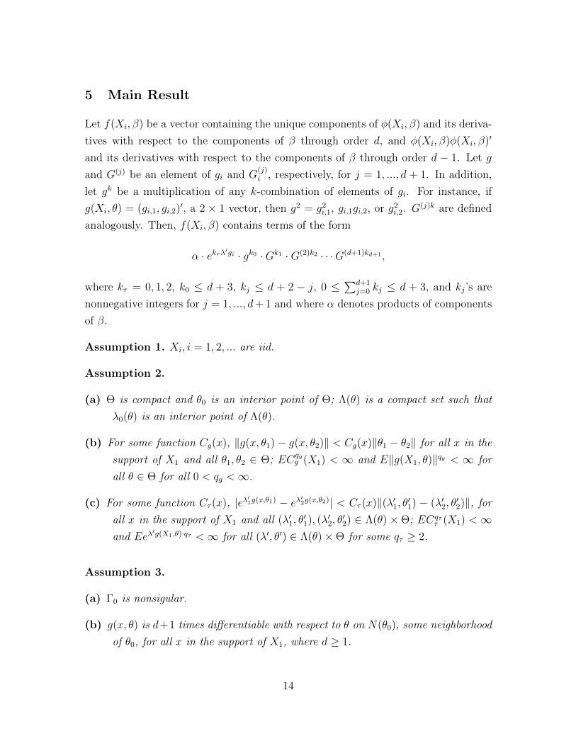
The first result holds by Lemma 2(b). To show the second result, we apply Schwarz matrix inequal-

ity3 to get

|λ(θ)′gn(θ)− λ0(θ)′Egi(θ)| ≤ ‖λ(θ)− λ0(θ)‖‖gn(θ)‖+ ‖λ0(θ)‖‖gn(θ)− Egi(θ)‖.

By Lemma 2(a), (c), Lemma 1(b) with p = qg, and the fact that λ0(θ) exists for all θ ∈ Θ and Θ is

compact, the second conclusion follows.

Since lnL(θ) is continuous and uniquely maximized at θ0, ∀ε > 0, ∃η > 0 such that ‖θ− θ0‖ > ε

implies that lnL(θ0)− lnL(θ) ≥ η > 0. By the triangle inequality, the fact that θ maximizes ln L(θ),

and (A.10),

P(‖θ − θ0‖ > ε

)≤ P

(lnL(θ0)− lnL(θ) ≤ η

)= P

(lnL(θ0)− ln L(θ) + ln L(θ)− lnL(θ) ≤ η

)≤ P

(lnL(θ0)− ln L(θ0) + ln L(θ)− lnL(θ) ≤ η

)≤ P

(supθ∈Θ

∣∣∣ln L(θ)− lnL(θ)∣∣∣ ≤ η/2) = o(n−a).

Thus, we have

limn→∞

naP(‖θ − θ0‖ > ε

)= 0. (A.11)

Next, we show

limn→∞

naP(‖λ(θ)− λ0(θ0)‖ > ε

)= 0. (A.12)

By the triangle inequality,

P(‖λ(θ)− λ0(θ0)‖ > ε

)≤ P

(‖λ(θ)− λ0(θ)‖ > ε/2

)+ P

(‖λ0(θ)− λ0(θ0)‖ > ε/2

)≤ P

(supθ∈Θ‖λ(θ)− λ0(θ)‖ > ε/2

)+ o(n−a) = o(n−a).

The last equality holds by Lemma 2(c). To see P(‖λ0(θ)− λ0(θ0)‖ > ε/2

)= o(n−a), let f(θ, λ) ≡

Eeλ′gi(θ)gi(θ), a continuously differentiable function on (Θ,Λ(θ)). Since f(θ0, λ0) = 0 and (∂/∂λ′)f(θ0, λ0) =

Eeλ′0gi(θ0)gi(θ0)gi(θ0)′ is invertible by Assumption 3(a), λ0(θ) is continuous in a neighborhood of θ0

by the implicit function theorem. By (A.11), θ is in a neighborhood of θ0 with probability 1−o(n−a)

and this implies that ‖λ0(θ)− λ0(θ0)‖ → 0 with probability 1− o(n−a). Thus, (A.12) is proved.

Next, we show

limn→∞

naP (‖τ − τ0‖ > ε) = 0. (A.13)

Write λ ≡ λ(θ) and λ0 ≡ λ0(θ0). Since τ = n−1∑ni=1 e

λ′gi(θ) and τ0 = Eeλ′0gi(θ0), (A.13) follows

3See Appendix A of Hansen (2011).

32

from

limn→∞

naP

(∣∣∣∣∣n−1n∑i=1

eλ′gi(θ) − n−1

n∑i=1

eλ′0gi(θ0)

∣∣∣∣∣ > ε

)= 0,

limn→∞

naP

(∣∣∣∣∣n−1n∑i=1

eλ′0gi(θ0) − Eeλ

′0gi(θ0)

∣∣∣∣∣ > ε

)= 0.

To show these results, we apply the argument with the proof of Lemma 2(b) that λ(θ) is in the

interior of Λ(θ) with probability 1 − o(n−a). Using this fact, Assumption 2(c), Lemma 1(b) with

h(Xi) = Cτ (Xi) and p = qτ , (A.11), and (A.12) prove the first result. The second result holds by

Lemma 1(a) with p = qτ .

Finally, we show

limn→∞

naP (‖κ− κ0‖ > ε) = 0. (A.14)

Since

κ = −

(n−1

n∑i=1

eλ′gi(θ)gi(θ)gi(θ)

′

)−1

τ gn(θ), and

κ0 = −(Eeλ

′0gi(θ0)gi(θ0)gi(θ0)′

)−1

τ0Egi(θ0),

(A.14) follows from

limn→∞

naP

(∥∥∥∥∥n−1n∑i=1

eλ′gi(θ)gi(θ)gi(θ)

′ − n−1n∑i=1

eλ′0gi(θ0)gi(θ0)gi(θ0)′

∥∥∥∥∥ > ε

)= 0, (A.15)

limn→∞

naP

(∥∥∥∥∥n−1n∑i=1

eλ′0gi(θ0)gi(θ0)gi(θ0)′ − Eeλ

′0gi(θ0)gi(θ0)gi(θ0)′

∥∥∥∥∥ > ε

)= 0, (A.16)

limn→∞

naP (‖τ − τ0‖ > ε) = 0, (A.17)

limn→∞

naP(‖gn(θ)− gn(θ0)‖ > ε

)= 0, (A.18)

limn→∞

naP (‖gn(θ0)− Egi(θ0)‖ > ε) = 0. (A.19)

The third result (A.17) holds by (A.13). The fourth result (A.18) holds by Assumption 2(b), Lemma

1(b) with h(Xi) = Cg(Xi) and p = qg, and (A.11). The last result (A.19) holds by Assumption 2(b)

and Lemma 1(a) with h(Xi) = gi(θ0)− Egi(θ0), c = 0 and p = qg.

To show the first result (A.15), we apply the triangle inequality to get∥∥∥∥∥n−1n∑i=1

(eλ′gi(θ)gi(θ)gi(θ)

′ − eλ′0gi(θ0)gi(θ0)gi(θ0)′

)∥∥∥∥∥≤

∥∥∥∥∥n−1n∑i=1

∣∣∣eλ′gi(θ) − eλ′0gi(θ0)∣∣∣ gi(θ)gi(θ)′

∥∥∥∥∥+

∥∥∥∥∥n−1n∑i=1

eλ′0gi(θ0)

(gi(θ)gi(θ)

′ − gi(θ0)gi(θ0)′)∥∥∥∥∥ . (A.20)

33

By Assumption 2(c), with probability 1− o(n−a), the first term of (A.20) satisfies∥∥∥∥∥n−1n∑i=1

∣∣∣eλ′gi(θ) − eλ′0gi(θ0)∣∣∣ gi(θ)gi(θ)′

∥∥∥∥∥ ≤∥∥∥∥∥n−1

n∑i=1

Cτ (Xi)gi(θ)gi(θ)′

∥∥∥∥∥·‖(λ′, θ′)′−(λ0, θ0)′‖ = op(1).

The last conclusion op(1) holds by (A.11), (A.12), and the fact that ‖n−1∑ni=1 Cτ (Xi)gi(θ)gi(θ)

′‖ =

Op(1) with probability 1−o(n−a), which can be proved as follows. By the triangle inequality, Schwarz

matrix inequality and Assumption 2(b),

‖gi(θ)gi(θ)′‖ ≤ ‖gi(θ)gi(θ)′ − gi(θ0)gi(θ0)′‖+ ‖gi(θ0)gi(θ0)′‖

≤ ‖(gi(θ)− gi(θ0))(gi(θ) + gi(θ0))′‖+ ‖gi(θ0)‖2

≤ ‖θ − θ0‖2C2g (Xi) + 2‖θ − θ0‖ · Cg(Xi)‖gi(θ0)‖+ ‖gi(θ0)‖2.

Using this inequality relation and the triangle inequality,∥∥∥∥∥n−1n∑i=1

Cτ (Xi)gi(θ)gi(θ)′

∥∥∥∥∥ ≤ n−1n∑i=1

Cτ (Xi)‖gi(θ0)‖2 + ‖θ − θ0‖2n−1n∑i=1

Cτ (Xi)C2g (Xi)

+2‖θ − θ0‖ · n−1n∑i=1

Cτ (Xi)Cg(Xi)‖gi(θ0)‖.

Then the right-hand-side is Op(1) with probability 1− o(n−a) by using (A.11) and applying Lemma

1(b) with h(Xi) = Cτ (Xi)‖gi(θ0)‖2, h(Xi) = Cτ (Xi)C2g (Xi), and h(Xi) = Cτ (Xi)Cg(Xi)‖gi(θ0)‖,

provided that E‖h(Xi)‖p <∞ for some p ≥ 2 and p > 2a. In order to satisfy this condition, we use

Holder’s inequality: for some ζ > 0,

ECpτ (Xi)‖gi(θ0)‖2p ≤(ECp(1+ζ)

τ (Xi))(1+ζ)−1

·(E‖gi(θ0)‖2p(1+ζ−1)

)ζ(1+ζ)−1

,

ECpτ (Xi)C2pg (Xi) ≤

(ECp(1+ζ)

τ (Xi))(1+ζ)−1

·(EC2p(1+ζ−1)

g

)ζ(1+ζ)−1

,

ECpτ (Xi)Cpg (Xi)‖gi(θ0)‖p ≤

(ECp(1+ζ)

τ (Xi))(1+ζ)−1

·(EC2p(1+ζ−1)

g

) ζ(1+ζ)−1

2 ·(E‖gi(θ0)‖2p(1+ζ−1)

) ζ(1+ζ)−1

2

,

where Cauchy-Schwarz inequality is further applied for the last result. Letting p(1 + ζ) = qτ gives

qτ ≥ 2(1+ζ) and qτ > 2a(1+ζ). Letting 2p(1+ζ−1) = qg gives qg ≥ 4(1+ζ−1) and qg > 4a(1+ζ−1).

These conditions are assumed in the present Lemma.

The second term of (A.20) can be proved similarly. By the triangle inequality, Schwarz matrix

inequality, and Assumption 2(b),∥∥∥∥∥n−1n∑i=1

eλ′0gi(θ0)(gi(θ)gi(θ)

′ − gi(θ0)gi(θ0)′)

∥∥∥∥∥≤ ‖θ − θ0‖2n−1

n∑i=1

eλ′0gi(θ0)C2

g (Xi) + 2‖θ − θ0‖ · n−1n∑i=1

eλ′0gi(θ0)Cg(Xi)‖gi(θ0)‖.

34

Then, (A.11) and Lemma 2(b) with h(Xi) = eλ′0gi(θ0)C2

g (Xi) and h(Xi) = eλ′0gi(θ0)Cg(Xi)‖gi(θ0)‖

give the desired result. This proves (A.15).

The result (A.16) can be proved by applying Lemma 1(a) with c = 0 and h(Xi) = eλ′0gi(θ0)gi(θ0)gi(θ0)′−

Eeλ′0gi(θ0)gi(θ0)gi(θ0)′. To see if h(Xi) satisfies the condition of Lemma 1(a), it suffices to show

Eeλ′0gi(θ0)·p‖gi(θ0)‖2p < ∞ by Minkowski’s inequality. But we already proved that the assumed qg

and qτ satisfy this condition in the present Lemma. Since we have shown (A.15)-(A.19), the result

(A.14) is proved and this completes the proof of the Lemma. Q.E.D.


Proof. β solves n−1∑ni=1 φ(Xi, β) = 0 with probability 1− o(n−a), because β is in the interior of B

with probability 1− o(n−a). By the mean value expansion of n−1∑ni=1 φ(Xi, β) = 0 around β0,

β − β0 = −

(n−1

n∑i=1

∂φ(Xi, β)

∂β′

)−1

n−1n∑i=1

φ(Xi, β0),

with probability 1− o(n−a), where β lies between β and β0 and may differ across rows. The Lemma

follows from

limn→∞

naP

(∥∥∥∥∥n−1n∑i=1

∂φ(Xi, β)

∂β′− n−1

n∑i=1

∂φ(Xi, β0)

∂β′

∥∥∥∥∥ > ε

)= 0, (A.21)

limn→∞

naP

(∥∥∥∥∥n−1n∑i=1

∂φ(Xi, β0)

∂β′− E∂φ(Xi, β0)

∂β′

∥∥∥∥∥ > ε

)= 0, (A.22)

limn→∞

naP

(∥∥∥∥∥n−1n∑i=1

φ(Xi, β0)

∥∥∥∥∥ > n−c

)= 0. (A.23)

First, we prove (A.23). We apply Lemma 1(a) with h(Xi) = φ(Xi, β0). To satisfy the con-

dition of Lemma 1(a), we need to show E‖φ(Xi, β0)‖p < ∞ for p ≥ 2 and p > 2a/(1 − 2c).

By investigating the elements of ‖φ(Xi, β0)‖, it suffices to show Eeλ′0gi(θ0)·p‖gi(θ0)‖2p < ∞ and

Eeλ′0gi(θ0)·p‖gi(θ0)‖p‖Gi(θ0)‖p < ∞. By Holder’s inequality and Cauchy-Schwarz inequality, we

have qg ≥ 4(1 + ζ−1) and qg > 4a(1− 2c)−1(1 + ζ−1), qτ ≥ 2(1 + ζ) and qτ > 2a(1− 2c)−1(1 + ζ),

and qG ≥ 4(1 + ζ−1) and qG > 4a(1− 2c)−1(1 + ζ−1). But this is implied by the assumption of the

Lemma.

Second, we prove (A.22). We apply Lemma 1(a) with h(Xi) = (∂/∂β′)φ(Xi, β0)−E(∂/∂β′)φ(Xi, β0)

and c = 0. By investigating the elements of ‖(∂/∂β′)φ(Xi, β0)‖, it suffices to show Eeλ′0gi(θ0)·p‖gi(θ0)‖3p <

∞, Eeλ′0gi(θ0)·p‖gi(θ0)‖2p‖Gi(θ0)‖p < ∞, and Eeλ

′0gi(θ0)·p‖gi(θ0)‖p‖Gi(θ0)‖2p < ∞, to satisfy the

condition of Lemma 1(a) with c = 0. By Holder’s inequality and Cauchy-Schwarz inequality, the

corresponding conditions for qg, qτ and qG are qg ≥ 6(1 + ζ−1) and qg > 6a(1 + ζ−1), qτ ≥ 2(1 + ζ)

and qτ > 2a(1+ζ), and qG ≥ 6(1+ζ−1) and qG > 6a(1+ζ−1), which are implied by the assumption

of the Lemma.

Finally, (A.21) can be proved by multiple applications of Lemma 1(b) and Lemma 3. Note that

35

the matrix (∂/∂β′)φ(Xi, β) consists of terms of the form α · ekτλ′gi(θ)g(θ)k0 · G(θ)k1 · G(2)(θ)k2 for

kτ = 0, 1, k0 = 0, 1, 2, 3, k1 = 0, 1, 2, k2 = 0, 1, and 0 ≤ k0 + k1 + k2 ≤ 3, where g(θ), G(θ), and

G(2)(θ) denote elements of gi(θ), Gi(θ), and G(2)i (θ), respectively, and where α denotes products of

elements of β that are necessarily bounded for β ∈ Bδ(β0). Thus, (∂/∂β′)φ(Xi, β)−(∂/∂β′)φ(Xi, β0)

consists of terms of the form

α · ekτ λ′gi(θ)g(θ)k0 ·G(θ)k1 ·G(2)(θ)k2 − α0 · ekτλ

′0gi(θ0)g(θ0)k0 ·G(θ0)k1 ·G(2)(θ0)k2

= (α− α0) · ekτ λ′gi(θ) · g(θ)k0 ·G(θ)k1 ·G(2)(θ)k2

+α0 ·(ekτ λ

′gi(θ) − ekτλ′0gi(θ0)

)· g(θ)k0 ·G(θ)k1 ·G(2)(θ)k2

+α0 · ekτλ′0gi(θ0) ·

(g(θ)k0 − g(θ0)k0

)·G(θ)k1 ·G(2)(θ)k2

+α0 · ekτλ′0gi(θ0) · g(θ0)k0

(G(θ)k1 −G(θ0)k1

)·G(2)(θ)k2

+α0 · ekτλ′0gi(θ0) · g(θ0)k0 ·G(θ0)k1

(G(2)(θ)k2 −G(2)(θ0)k2

). (A.24)

We apply Lemma 3 to show P (|α − α0| > ε) = o(n−a). By Assumption 2(b)-(c), Assumption 3(c),

Lemma 1(b) and Lemma 3,

ekτ λ′gi(θ) · g(θ)k0 ·G(θ)k1 ·G(2)(θ)k2 ≤ ekτλ

′0gi(θ0) · |g(θ0)|k0 · |G(θ0)|k1 · |G(2)(θ0)|k2 + op(1).

To apply Lemma 1(b) to the first term of the right-hand side of the above inequality, it suffices to

show Eeλ′0gi(θ0)·p · |g(θ0)|3p < ∞, Eeλ

′0gi(θ0)·p · |g(θ0)|2p · |G(θ0)|p < ∞, and Eeλ

′0gi(θ0)·p · |g(θ0)|p ·

|G(θ0)|p · |G(2)(θ0)|p <∞ for p ≥ 2 and p > 2a. Since we already showed this in the proof of (A.22),

the first term of (A.24) is op(1). Similarly, we can show the remaining terms of (A.24) are also op(1)

by the binomial theorem under the assumption of the Lemma, and thus, (A.21) is proved.

We illustrate the above proof for a term of (∂/∂β′)φ(Xi, β) − (∂/∂β′)φ(Xi, β0). For example,

we show

limn→∞

naP

(∥∥∥∥∥n−1n∑i=1

eλ(θ)′gi(θ)gi(θ)gi(θ)′κgi(θ)

′ − n−1n∑i=1

eλ0(θ0)′gi(θ0)gi(θ0)gi(θ0)′κ0gi(θ0)′

∥∥∥∥∥ > ε

)= 0,

as follows. By Assumption 2, and the triangle and Schwarz matrix inequalities,∥∥∥∥∥n−1n∑i=1

eλ(θ)′gi(θ)gi(θ)gi(θ)′κgi(θ)

′ − n−1n∑i=1

eλ0(θ0)′gi(θ0)gi(θ0)gi(θ0)′κ0gi(θ0)′

∥∥∥∥∥≤ ‖κ‖ · ‖(λ′, θ′)− (λ′0, θ

′0)‖n−1

n∑i=1

Cτ (Xi)‖gi(θ)‖3

+‖κ‖ · n−1n∑i=1

eλ′0gi(θ0)‖gi(θ)gi(θ)′ − gi(θ0)gi(θ0)′‖ · ‖gi(θ)‖

+‖κ− κ0‖ · n−1n∑i=1

eλ′0gi(θ0)‖gi(θ)‖2 · ‖gi(θ)‖+ ‖κ0‖‖θ − θ0‖n−1

n∑i=1

eλ′0gi(θ0)Cg(Xi)‖gi(θ)‖2.

36

The conclusion follows from multiple applications of Lemma 1(b), Lemma 3, and the following

inequality relations:

‖κ‖ ≤ ‖κ− κ0‖+ ‖κ0‖,

‖gi(θ)‖ ≤ Cg(Xi)‖θ − θ0‖+ ‖gi(θ0)‖,

‖gi(θ)gi(θ)′ − gi(θ0)gi(θ0)′‖ ≤ C2g (Xi)‖θ − θ0‖2 + 2Cg(Xi)‖θ − θ0‖ · ‖gi(θ0)‖.

Q.E.D.


Proof. See the proof of Lemma 5 of Andrews (2002). Q.E.D.


Proof. See the proof of Lemma 6 of Andrews (2002). Q.E.D.


Proof. The result (a) is proved by the proof of Lemma 7 of Lee (2011), that also mimics the proof of

Lemma 8 of Hall and Horowitz (1996). We apply Lemma 6 with c = 0 and p = qg using Assumption

2(b).

Proving (b) and (c) involves several steps. We first show

limn→∞

naP

(P ∗

(sup

(λ′,θ′)∈Λ(θ)×Θ

∣∣∣∣∣n−1n∑i=1

(eλ(θ)′g∗i (θ) − eλ(θ)′gi(θ)

)∣∣∣∣∣ > ε

)> n−a

)= 0. (A.25)

The proof of (A.25) is similar to that of Lemma 7 of Lee (2011), that mimics the proof of Lemma 8

of Hall and Horowitz (1996). We apply our Lemma 6(c) with c = 0, h(Xi) = eλ′jgi(θj) − Eeλ

′jgi(θj)

for some (λ′j , θ′j) ∈ Λ(θ) × Θ or h(Xi) = Cτ (Xi) − ECτ (Xi), and p = qτ . Note that qτ needs

to satisfy qτ ≥ 2 and qτ > 4a. To see this works, observe that h(X∗i ) = eλ′jg∗i (θj) − Eeλ

′jgi(θj) or

h(X∗i ) = Cτ (X∗i ) − ECτ (Xi). Then, E∗h(X∗i ) = n−1∑ni=1 e

λ′jgi(θj) − Eeλ′jgi(θj) or E∗h(X∗i ) =

n−1∑ni=1 Cτ (Xi)− ECτ (Xi). Thus,

h(X∗i )− E∗h(X∗i ) = eλ′jg∗i (θj) − n−1

n∑i=1

eλ′jgi(θj) or

h(X∗i )− E∗h(X∗i ) = Cτ (X∗i )− n−1n∑i=1

Cτ (Xi).

Next, we show

limn→∞

naP

(P ∗(

supθ∈Θ

∥∥λ∗(θ)− λ(θ)∥∥ > ε

)> n−a

)= 0, (A.26)

37

where λ∗(θ) = arg minλ∈Λ(θ) n−1∑ni=1 e

λ′g∗i (θ). For a given ε > 0, let

η = infθ∈Θ

infλ∈Λ(θ)

‖λ−λ(θ)‖>ε

(n−1n∑i=1

eλ′gi(θ) − n−1

n∑i=1

eλ(θ)′gi(θ)),

which is positive by the strict convexity of n−1∑ni=1 e

λ′gi(θ) in λ, λ(θ) ≡ arg minλ∈Λ(θ) n−1∑ni=1 e

λ′gi(θ),

and the fact that Θ is compact. By the definition of η,

P ∗

(supθ∈Θ

(n−1

n∑i=1

eλ∗(θ)′gi(θ) − n−1

n∑i=1

eλ(θ)′gi(θ)

)≤ η

)≤ P ∗

(supθ∈Θ‖λ∗(θ)− λ(θ)‖ ≤ ε

). (A.27)

Since n−1∑ni=1 e

λ∗(θ)′g∗i (θ) − n−1∑ni=1 e

λ(θ)′g∗i (θ) < 0,

supθ∈Θ

(n−1

n∑i=1

eλ∗(θ)′gi(θ) − n−1

n∑i=1

eλ(θ)′gi(θ)

)

≤ supθ∈Θ

(n−1

n∑i=1

eλ∗(θ)′gi(θ) − n−1

n∑i=1

eλ∗(θ)′g∗i (θ)

)+ supθ∈Θ

(n−1

n∑i=1

eλ∗(θ)′g∗i (θ) − n−1

n∑i=1

eλ(θ)′g∗i (θ)

)

+ supθ∈Θ

(n−1

n∑i=1

eλ(θ)′g∗i (θ) − n−1n∑i=1

eλ(θ)′gi(θ)

)

≤ 2 sup(λ′,θ′)′∈Λ(θ)×Θ

∣∣∣∣∣n−1n∑i=1

eλ′g∗i (θ) − Eeλ

′gi(θ)

∣∣∣∣∣ .Thus, we have

P ∗

(supθ∈Θ

(n−1

n∑i=1

eλ∗(θ)′gi(θ) − n−1

n∑i=1

eλ(θ)′gi(θ)

)≤ η

)

≥ P ∗

(sup

(λ′,θ′)′∈Λ(θ)×Θ

∣∣∣∣∣n−1n∑i=1

eλ′g∗i (θ) − n−1

n∑i=1

eλ′gi(θ)

∣∣∣∣∣ ≤ η/2),

and this implies that

P

(P ∗

(supθ∈Θ

(n−1

n∑i=1

eλ∗(θ)′gi(θ) − n−1

n∑i=1

eλ(θ)′gi(θ)

)> η

)> n−a

)

≤ P

(P ∗

(sup

(λ′,θ′)′∈Λ(θ)×Θ

∣∣∣∣∣n−1n∑i=1

eλ′g∗i (θ) − n−1

n∑i=1

eλ′gi(θ)

∣∣∣∣∣ > η/2

)> n−a

)= o(n−a),

by (A.25). Using this result, (A.27) implies (A.26).

To prove the present Lemma (c), we need to replace λ∗(θ) and λ(θ) with λ∗(θ) and λ(θ),

respectively. We have shown that λ(θ) = λ(θ) in the event that λ(θ) ∈ int(Λ(θ)) in the proof of

Lemma 2. By similar argument, λ∗(θ) = λ∗(θ) in the event that λ∗(θ) ∈ int(Λ(θ)). Take a closed

neighborhood Nδ(λ0(θ)) of radius δ around λ0(θ) such that Nδ(λ0(θ)) ⊂ int(Λ(θ)). Then, whenever

38

λ(θ), λ∗(θ) ∈ int(Λ(θ)), ‖λ(θ)− λ0(θ)‖ ≤ δ and ‖λ∗(θ)− λ0(θ)‖ ≤ δ for all θ ∈ Θ. We use this fact

to prove the present Lemma (c). By the triangle inequality,

‖λ∗(θ)− λ0(θ)‖ ≤ ‖λ∗(θ)− λ(θ)‖+ ‖λ(θ)− λ0(θ)‖,

and thus we have

P

(P ∗(

supθ∈Θ‖λ∗(θ)− λ0(θ)‖ > δ

)> n−a

)≤ P

(P ∗(

supθ∈Θ‖λ∗(θ)− λ(θ)‖ > δ/2

)> n−a

)+ P

(P ∗(

supθ∈Θ‖λ(θ)− λ0(θ)‖ > δ/2

)> n−a

)= o(n−a) + o(n−a) = o(n−a), (A.28)

by (A.26) and (A.6). Note that λ(θ) is calculated from the original sample and thus

P

(P ∗(


)> n−a

)= P

(1


> n−a

)= P

(1


> n−a, sup

θ∈Θ‖λ(θ)− λ0(θ)‖ > δ/2

)+P

(1


> n−a, sup

θ∈Θ‖λ(θ)− λ0(θ)‖ ≤ δ/2

)≤ P

(supθ∈Θ‖λ(θ)− λ0(θ)‖ > δ/2

)= o(n−a), (A.29)

where 1· is an indicator function. Now, we are ready to prove the present Lemma (c):

P ∗(

supθ∈Θ

∥∥∥λ∗(θ)− λ(θ)∥∥∥ > ε

)= P ∗

(supθ∈Θ

∥∥∥λ∗(θ)− λ(θ)∥∥∥ > ε, sup

θ∈Θ‖λ∗(θ)− λ0(θ)‖ > δ

)+P ∗

(supθ∈Θ

∥∥∥λ∗(θ)− λ(θ)∥∥∥ > ε, sup

θ∈Θ‖λ∗(θ)− λ0(θ)‖ ≤ δ

)≤ P ∗

(supθ∈Θ‖λ∗(θ)− λ0(θ)‖ > δ

)+ P ∗

(supθ∈Θ‖λ(θ)− λ0(θ)‖ > δ

)+ P ∗

(supθ∈Θ

∥∥λ∗(θ)− λ(θ)∥∥ > ε

),

and thus,

P

(P ∗(

supθ∈Θ

∥∥∥λ∗(θ)− λ(θ)∥∥∥ > ε

)> n−a

)≤ P

(P ∗(

supθ∈Θ‖λ∗(θ)− λ0(θ)‖ > δ

)>n−a

3

)+ P

(P ∗(

supθ∈Θ‖λ(θ)− λ0(θ)‖ > δ

)>n−a

3

)+P

(P ∗(

supθ∈Θ

∥∥λ∗(θ)− λ(θ)∥∥ > ε

)>n−a

3

)= o(n−a),

39

by (A.28), (A.29), and (A.26).

Finally, the present Lemma (b) follows from the results below:

limn→∞

naP

(P ∗

(supθ∈Θ

∣∣∣∣∣n−1n∑i=1

(eλ∗(θ)′g∗i (θ) − eλ(θ)′g∗i (θ)

)∣∣∣∣∣ > ε

)> n−a

)= 0, (A.30)

limn→∞

naP

(P ∗

(supθ∈Θ

∣∣∣∣∣n−1n∑i=1

(eλ(θ)′g∗i (θ) − eλ(θ)′gi(θ)

)∣∣∣∣∣ > ε

)> n−a

)= 0. (A.31)

Since λ(θ) ∈ int(Λ(θ)) with probability 1−o(n−a) as in (A.29), (A.31) follows from (A.25). To show

(A.30), we use the arguments used in the proof of the present Lemma:

P

(P ∗

(supθ∈Θ

∣∣∣∣∣n−1n∑i=1

(eλ∗(θ)′g∗i (θ) − eλ(θ)′g∗i (θ)

)∣∣∣∣∣ > ε

)> n−a

)

≤ P

(P ∗

(supθ∈Θ

∣∣∣∣∣n−1n∑i=1

(eλ∗(θ)′g∗i (θ) − eλ(θ)′g∗i (θ)

)∣∣∣∣∣ > ε

)> n−a

)

+P

(P ∗(

supθ∈Θ

∥∥λ∗(θ)− λ0(θ)∥∥ > δ

)> n−a

)+ P

(P ∗(

supθ∈Θ

∥∥λ(θ)− λ0(θ)∥∥ > δ

)> n−a

)≤ o(n−a) + P

(P ∗

(supθ∈Θ

∥∥λ∗(θ)− λ0(θ)∥∥n−1

n∑i=1

Cτ (X∗i ) > ε

)> n−a

)= o(n−a),

by applying Lemma 6(d) with h(X∗i ) = Cτ (X∗i ) and p = qτ and using (A.26), (A.28), and (A.29).

Q.E.D.


Proof. The proof is analogous to that of Lemma 3. Though they are similar, the proof involves some

additional steps for the bootstrap version of the estimators. First, we show

limn→∞

naP

(P ∗(

supθ∈Θ| ln L∗(θ)− ln L(θ)| > ε

)> n−a

)= 0. (A.32)

Since

ln L∗(θ) = − ln

(n−1

n∑i=1

eλ∗(θ)′g∗i (θ)

)+ λ∗(θ)′g∗n(θ),

(A.32) follows from

limn→∞

naP

(P ∗

(supθ∈Θ|n−1

n∑i=1

(eλ∗(θ)′g∗i (θ) − eλ(θ)′gi(θ)

)| > ε

)> n−a

)= 0,

limn→∞

naP

(P ∗(

supθ∈Θ|λ∗(θ)′g∗n(θ)− λ(θ)′gn(θ)| > ε

)> n−a

)= 0.

40

Since the assumption of the present Lemma implies that qg ≥ 2, qg > 4a, qτ ≥ 2, and qτ > 4a, the

first result holds by Lemma 7(b). To show the second result, we apply Schwarz matrix inequality to

get

supθ∈Θ|λ∗(θ)′g∗n(θ)− λ(θ)′gn(θ)| ≤ sup

θ∈Θ‖λ∗(θ)− λ(θ)‖ · sup

θ∈Θ‖g∗n(θ)‖+ sup

θ∈Θ‖λ(θ)‖ · sup

θ∈Θ‖g∗n(θ)− gn(θ)‖.

By Lemma 7(a), (c), Lemma 6(d) with h(X∗i ) = supθ∈Θ ‖g∗i (θ)‖ and p = qg, the inequality ‖λ(θ)‖ ≤‖λ(θ)−λ0(θ)‖+‖λ0(θ)‖, Lemma 2(c), and the fact that λ0(θ) exists for all θ ∈ Θ and Θ is compact,

the second conclusion follows.

Next we claim that given ε > 0, there exists η > 0 independent of n such that ‖θ − θ‖ > ε

implies that ln L(θ) − ln L(θ) ≥ η > 0 with probability 1 − o(n−a). To show this claim, define

M = infθ∈Nε(θ)c∩Θ(lnL(θ0) − lnL(θ)), where Nε(θ) = θ : ‖θ − θ‖ < ε. Then, M > 0 if ‖θ −θ0‖ ≤ ε. Now, conditional on the event that ‖θ − θ0‖ ≤ ε, supθ∈Θ | ln L(θ) − lnL(θ)| ≤ M/6, and

lnL(θ0)− lnL(θ) ≤M/3, we have

ln L(θ)− ln L(θ) = lnL(θ0)− lnL(θ) + ln L(θ)− ln L(θ)− lnL(θ0) + lnL(θ) + lnL(θ)− lnL(θ)

≥ lnL(θ0)− lnL(θ)− | ln L(θ)− lnL(θ) + lnL(θ)− ln L(θ)| − (lnL(θ0)− lnL(θ))

≥ M − 2 supθ∈Θ| lnL(θ)− ln L(θ)| − (lnL(θ0)− lnL(θ))

≥ M/3 > 0,

for any ‖θ − θ‖ > ε. Since the event occurs with probability 1 − o(n−a) by Lemma 3, this proves

the claim.

By the claim, the triangle inequality, the fact that θ∗ maximizes ln L∗(θ), and (A.32),

P(P ∗(‖θ − θ0‖ > ε

)> n−a

)≤ P

(P ∗(

ln L(θ)− ln L(θ∗) ≤ η)> n−a

)= P

(P ∗(

ln L(θ)− ln L∗(θ∗) + ln L∗(θ∗)− ln L(θ∗) ≤ η)> n−a

)≤ P

(P ∗(

ln L(θ)− ln L∗(θ) + ln L∗(θ∗)− ln L(θ∗) ≤ η)> n−a

)≤ P

(P ∗(

supθ∈Θ

∣∣∣ln L∗(θ)− ln L(θ)∣∣∣ ≤ η/2) > n−a

)= o(n−a).

Thus, we have

limn→∞

naP(P ∗(‖θ∗ − θ‖ > ε

)> n−a

)= 0. (A.33)

Next, we show

limn→∞

naP(P ∗(‖λ∗(θ∗)− λ(θ)‖ > ε

)> n−a

)= 0. (A.34)

41

By the triangle inequality,

P ∗(‖λ∗(θ∗)− λ(θ)‖ > ε

)≤ P ∗

(‖λ∗(θ∗)− λ(θ∗)‖ > ε

4

)+ P ∗

(‖λ(θ∗)− λ0(θ∗)‖ > ε

4

)+P ∗

(‖λ0(θ∗)− λ0(θ)‖ > ε

4

)+ P ∗

(‖λ0(θ)− λ(θ)‖ > ε

4

)≤ P ∗

(supθ∈Θ‖λ∗(θ)− λ(θ)‖ > ε

4

)+ P ∗

(‖λ0(θ∗)− λ0(θ)‖ > ε

4

)+2P ∗

(supθ∈Θ‖λ0(θ)− λ(θ)‖ > ε

4

).

Since ‖θ∗ − θ0‖ ≤ ‖θ∗ − θ‖+ ‖θ − θ0‖,

P(P ∗(‖θ∗ − θ0‖ > ε

)> n−a

)≤ P

(P ∗(‖θ∗ − θ‖ > ε

)> n−a

)+ P

(‖θ − θ0‖ > ε

)= o(n−a), (A.35)

by Lemma 3 and (A.33). Therefore, (A.34) follows from Lemma 7(c), Lemma 2(c), the fact that

λ0(θ) is continuous in a neighborhood of θ0, and (A.35).

Next, we show

limn→∞

naP(P ∗ (‖τ∗ − τ‖ > ε) > n−a

)= 0. (A.36)

Since τ∗ = n−1∑ni=1 e

λ∗′g∗i (θ∗), where λ∗ ≡ λ∗(θ∗), (A.36) follows from

limn→∞

naP

(P ∗

(∣∣∣∣∣n−1n∑i=1

(eλ∗′g∗i (θ∗) − eλ

′g∗i (θ))∣∣∣∣∣ > ε

)> n−a

)= 0,

limn→∞

naP

(P ∗

(∣∣∣∣∣n−1n∑i=1

(eλ′g∗i (θ) − eλ

′gi(θ))∣∣∣∣∣ > ε

)> n−a

)= 0.

Since λ∗ is in the interior of Λ(θ) with P ∗ probability 1−o(n−a) except, possibly, if χ is in a set of P

probability o(n−a) by (A.34), we use Assumption 2(c) and apply Lemma 6(d) with h(X∗i ) = Cτ (X∗i )

and p = qτ to show the first result. For the second result, we use the triangle inequality to get

eλ′g∗i (θ) − eλ

′gi(θ) ≤∣∣∣eλ′0g∗i (θ0) − eλ

′0gi(θ0)

∣∣∣+∣∣∣eλ′g∗i (θ) − eλ

′0g∗i (θ0)

∣∣∣+∣∣∣eλ′0gi(θ0) − eλ

′gi(θ)∣∣∣ ,

and apply Assumption 2(c), Lemma 6(a) with h(X∗i ) = eλ′0gi(θ0) − Eeλ′0gi(θ0), c = 0 and p = qτ ,

Lemma 6(d) with h(X∗i ) = Cτ (X∗i ) and p = qτ , Lemma 1(b) with h(Xi) = Cτ (Xi), and Lemma 3.

Finally, we show

limn→∞

naP(P ∗ (‖κ∗ − κ‖ > ε) > n−a

)= 0. (A.37)

Since

κ∗ = −

(n−1

n∑i=1

eλ∗′g∗i (θ∗)g∗i (θ∗)g∗i (θ∗)′

)−1

τ∗g∗n(θ∗),

42

(A.37) follows from

limn→∞

naP

(P ∗

(∥∥∥∥∥n−1n∑i=1

(eλ∗′g∗i (θ∗)g∗i (θ∗)g∗i (θ∗)′ − eλ

′g∗i (θ)g∗i (θ)g∗i (θ)′)∥∥∥∥∥ > ε

)> n−a

)= 0,

limn→∞

naP

(P ∗

(∥∥∥∥∥n−1n∑i=1

(eλ′g∗i (θ)g∗i (θ)g∗i (θ)′ − eλ

′g∗i (θ)g∗i (θ)g∗i (θ)′)∥∥∥∥∥ > ε

)> n−a

)= 0,

limn→∞

naP(P ∗ (‖τ∗ − τ‖ > ε) > n−a

)= 0,

limn→∞

naP(P ∗(‖g∗n(θ∗)− g∗n(θ)‖ > ε

)> n−a

)= 0,

limn→∞

naP(P ∗(‖g∗n(θ)− gn(θ)‖ > ε

)> n−a

)= 0.

Given the results proved in the present Lemma, these results can be proved in a similar fashion with

the proof of Lemma 3 and thus omitted. In particular, we apply Lemma 6 multiple times and we

need qg and qτ to be such that qg ≥ 4(1 + ζ−1), qg > 8a(1 + ζ−1), qτ ≥ 2(1 + ζ), and qτ > 4a(1 + ζ).

This is satisfied by the assumption of the Lemma. Q.E.D.


Proof. β∗ solves n−1∑ni=1 φ(X∗i , β

∗) = 0 with P ∗ probability 1 − o(n−a), except, possibly, if χ

is in a set of P probability o(n−a), because β∗ is in the interior of B with P ∗ probability 1 −o(n−a), except, possibly, if χ is in a set of P probability o(n−a). By the mean value expansion of

n−1∑ni=1 φ(X∗i , β

∗) = 0 around β,

β∗ − β = −

(n−1

n∑i=1

∂φ(X∗i , β∗)

∂β′

)−1

n−1n∑i=1

φ(X∗i , β),

with P ∗ probability 1− o(n−a), except, possibly, if χ is in a set of P probability o(n−a), where β∗

lies between β∗ and β and may differ across rows. The Lemma follows from

limn→∞

naP

(P ∗

(∥∥∥∥∥n−1n∑i=1

(∂φ(X∗i , β

∗)

∂β′− ∂φ(X∗i , β0)

∂β′

)∥∥∥∥∥ > ε

)> n−a

)= 0, (A.38)

limn→∞

naP

(P ∗

(∥∥∥∥∥n−1n∑i=1

(∂φ(X∗i , β0)

∂β′− E∂φ(Xi, β0)

∂β′

)∥∥∥∥∥ > ε

)> n−a

)= 0, (A.39)

limn→∞

naP

(P ∗

(∥∥∥∥∥n−1n∑i=1

φ(X∗i , β)

∥∥∥∥∥ > n−c

)> n−a

)= 0. (A.40)

First, we show (A.38). The proof is analogous to that of (A.21) in Lemma 4. We use Lemmas

3, 8, 6(d), and the inequality relation ‖β∗ − β0‖ ≤ ‖β∗ − β‖+ ‖β − β0‖. In order to apply Lemma

6(d) instead of Lemma 1(b) as in the proof of Lemma 4, we impose stronger assumption of qg, qG,

and qτ . In particular, qg, qG ≥ 6(1 + ζ−1), qg, qG > 12a(1 + ζ−1), qτ ≥ 2(1 + ζ), and qτ ≥ 4a(1 + ζ).

These are implied by the assumption of the Lemma.

43

The proof of (A.39) is also analogous to that of (A.22) in Lemma 4. We apply Lemma 6(c)

h(X∗i ) = (∂/∂β′)φ(X∗i , β0) − E(∂/∂β′)φ(Xi, β0) and c = 0. We need qg, qG ≥ 6(1 + ζ−1), qg, qG >

12a(1+ ζ−1), qτ ≥ 2(1+ ζ), and qτ ≥ 4a(1+ ζ), which are implied by the assumption of the Lemma.

Finally, we show (A.40). By the triangle inequality and the mean value expansion,∥∥∥∥∥n−1n∑i=1

φ(X∗i , β)

∥∥∥∥∥ ≤

∥∥∥∥∥n−1n∑i=1

φ(X∗i , β0)

∥∥∥∥∥+

∥∥∥∥∥n−1n∑i=1

∂φ(X∗i , β)

∂β′

∥∥∥∥∥ · ‖β − β0‖, and∥∥∥∥∥n−1n∑i=1

∂φ(X∗i , β)

∂β′

∥∥∥∥∥ ≤

∥∥∥∥∥n−1n∑i=1

∂φ(X∗i , β0)

∂β′

∥∥∥∥∥+

∥∥∥∥∥n−1n∑i=1

(∂φ(X∗i , β)

∂β′− ∂φ(X∗i , β0)

∂β′

)∥∥∥∥∥ ,where β lies between β and β0 and may differ across rows. Since ‖β − β0‖ ≤ ‖β − β0‖, the proof of

(A.38) and (A.39) can be applied to show

P

(P ∗

(∥∥∥∥∥n−1n∑i=1

∂φ(X∗i , β)

∂β′

∥∥∥∥∥ > K

)> n−a

)= o(n−a),

by Lemma 1(b) for some constant K > 0 and Lemma 3. Now, (A.40) follows from

P

(P ∗

(∥∥∥∥∥n−1n∑i=1

φ(X∗i , β0)

∥∥∥∥∥ > n−c

2

)> n−a

)= o(n−a), (A.41)

P

(P ∗(∥∥∥β − β0

∥∥∥ > n−c

2

)> n−a

)= o(n−a). (A.42)

To show (A.41), we apply Lemma 6(c) with h(X∗i ) = φ(X∗i , β0). To satisfy the condition of Lemma

6(c), we need to show E‖φ(Xi, β0)‖p <∞ for p ≥ 2 and p > 4a/(1− 2c). By investigating the ele-

ments of ‖φ(Xi, β0)‖, it suffices to show Eeλ′0gi(θ0)·p‖gi(θ0)‖2p <∞ and Eeλ

′0gi(θ0)·p‖gi(θ0)‖p‖Gi(θ0)‖p <

∞. By Holder’s inequality and Cauchy-Schwarz inequality, we have qg, qG ≥ 4(1 + ζ−1) and

qg, qG > 8a(1 − 2c)−1(1 + ζ−1), and qτ ≥ 2(1 + ζ) and qτ > 4a(1 − 2c)−1(1 + ζ). But this is

also implied by the assumption of the Lemma. (A.42) holds by Lemma 4 because

P

(P ∗(∥∥∥β − β0

∥∥∥ > n−c

2

)> n−a

)= P

(1

∥∥∥β − β0

∥∥∥ > n−c

2

> n−a,

∥∥∥β − β0

∥∥∥ > n−c

2

)+P

(1

∥∥∥β − β0

∥∥∥ > n−c

2

> n−a,

∥∥∥β − β0

∥∥∥ ≤ n−c

2

)≤ P

(∥∥∥β − β0

∥∥∥ > n−c

2

)= o(n−a).

Q.E.D.


Proof of (a). The proof is similar to the proof of (A.21) in Lemma 4 and is given by as follows. Since

f(Xi, β) consists of terms of the form α · ekτλ′gi(θ)g(θ)k0 ·G(θ)k1 · · ·G(d)(θ)kd , f(Xi, β)− f(Xi, β0)

44

consists of terms of the form

α · ekτλ′gi(θ)g(θ)k0 ·G(θ)k1 · · ·G(d+1)(θ)kd+1 − α0 · ekτλ

′0gi(θ0)g(θ0)k0 ·G(θ0)k1 · · ·G(d+1)(θ0)kd+1

= (α− α0) · ekτλ′gi(θ) · g(θ)k0 ·G(θ)k1 · · ·G(d+1)(θ)kd+1

+α0 ·(ekτλ

′gi(θ) − ekτλ′0gi(θ0)

)· g(θ)k0 ·G(θ)k1 · · ·G(d+1)(θ)kd+1

+α0 · ekτλ′0gi(θ0) ·

(g(θ)k0 − g(θ0)k0

)·G(θ)k1 · · ·G(d+1)(θ)kd+1

+α0 · ekτλ′0gi(θ0) · g(θ0)k0

(G(θ)k1 −G(θ0)k1

)· · ·G(d+1)(θ)kd+1

+α0 · ekτλ′0gi(θ0) · g(θ0)k0 ·G(θ0)k1 · · ·

(G(d+1)(θ)kd+1 −G(d+1)(θ0)kd+1

).

Since α is a product of elements of β, we can write (α−α0) ≤M‖β−β0‖ for some constant M <∞.

Let kτ = 2, which is the most restrictive case. By Assumption 2(c),

e2λ′gi(θ) − e2λ′0gi(θ0) =(eλ′gi(θ) − eλ

′0gi(θ0) + eλ

′0gi(θ0)

)2

− e2λ′0gi(θ0)

=(eλ′gi(θ) − eλ

′0gi(θ0)

)2

+ 2(eλ′gi(θ) − eλ

′0gi(θ0)

)· eλ

′0gi(θ0)

≤ C2τ (Xi) ‖(λ′, θ′)′ − (λ′0, θ

′0)′‖2 + 2Cτ (Xi) · eλ

′0gi(θ0) ‖(λ′, θ′)′ − (λ′0, θ

′0)′‖

≤ ‖β − β0‖ ·(C2τ (Xi)‖β − β0‖+ 2Cτ (Xi) · eλ

′0gi(θ0)

).

By the binomial theorem,

g(θ)k0 − g(θ0)k0 = (g(θ)− g(θ0) + g(θ0))k0 − g(θ0)k0

=

k0∑r=1

(k0

r

)(g(θ)− g(θ0))rg(θ0)k0−r

≤k0∑r=1

(k0

r

)Crg (Xi) · ‖θ − θ0‖r · ‖gi(θ0)‖k0−r

≤ ‖β − β0‖ ·k0∑r=1

(k0

r

)Crg (Xi) · ‖θ − θ0‖r−1 · ‖gi(θ0)‖k0−r.

Similarly, we can show G(j)(θ)kj − G(j)(θ0)kj ≤ ‖β − β0‖ · C(j)(Xi) for some C(j)(Xi) and for

j = 1, ..., d.

Now we can write f(Xi, β)− f(Xi, β0) ≤ C(Xi)‖β − β0‖, where

C(Xi) = Mekτλ′gi(θ) · · ·G(d+1)(θ)kd+1

+α0

(C2τ (Xi)‖β − β0‖+ 2Cτ (Xi) · eλ

′0gi(θ0)

)g(θ)k0 · · ·G(d+1)(θ)kd+1

+α0ekτλ′0gi(θ0)g(θ0)k0C(1)(Xi) + · · · .

To show C(Xi) is bounded with probability 1−o(n−a), as is in the proof of Lemma 4, the remaining

quantities such as ekτλ′gi(θ)·g(θ)k0 ·G(θ)k1 · · ·G(d+1)(θ)kd+1 , Ckττ (Xi)C

k0g (Xi), or Ckττ (Xi)C

∑d+1j=1 kj

G (Xi),

need to be shown to be bounded with probability 1 − o(n−a) by applying Lemma 1(b). It suffices

45

to show the most restrictive cases: EC2pτ (Xi)C

(d+3)pg (Xi) <∞ and EC2p

τ (Xi)C(d+3)pG (Xi) <∞ for

p ≥ 2 and p > 2a. By Holder’s inequality, for ζ > 0,

EC2pτ (Xi)C

(d+3)pg (Xi) ≤

(EC2p(1+ζ)

τ (Xi))(1+ζ)−1

·(EC(d+3)p(1+ζ−1)

g (Xi))ζ(1+ζ)−1

,

EC2pτ (Xi)C

(d+3)pG (Xi) ≤

(EC2p(1+ζ)

τ (Xi))(1+ζ)−1

·(EC

(d+3)p(1+ζ−1)G (Xi)

)ζ(1+ζ)−1

,

and the assumption on qg, qG, and qτ of the present Lemma satisfy the condition. Thus, the present

Lemma (a) is proved.

Proof of (b). The proof is analogous to that of the present Lemma (a), except that we use Lemma

6(d) in place of Lemma 1(b). Since Lemma 6(d) requires p ≥ 2 and p > 4a, we need stronger

conditions for qg, qG, and qτ , as are assumed. Q.E.D.


Proof of (a). By the definitions of Sn and S, it suffices to show

P

(∥∥∥∥∥n−1n∑i=1

f(Xi, β0)− Ef(Xi, β0)

∥∥∥∥∥ > ε

)= o(n−a).

We apply Lemma 1(a) with c = 0 and h(Xi) = f(Xi, β0)−Ef(Xi, β0). By investigating the compo-

nents of f(Xi, β0), the most restrictive condition for Lemma 1(a) to hold is Eeλ′0gi(θ0)·2pC

(d+3)pg (Xi) <

∞ and Eeλ′0gi(θ0)·2pC

(d+3)pG (Xi) <∞, where p ≥ 2 and p > 2a. By Holder’s inequality and Assump-

tions 2(b)-(c) and 3, we need qg, qG ≥ 2(d+ 3)(1 + ζ−1), qg, qG > 2a(d+ 3)(1 + ζ−1), qτ ≥ 4(1 + ζ)

and qτ > 4a(1 + ζ). But these are implied by the assumption of the Lemma.

Proof of (b). By the definitions of S∗n and S∗, it suffices to show

P

(P ∗

(∥∥∥∥∥n−1n∑i=1

f(X∗i , β)− n−1n∑i=1

f(Xi, β)

∥∥∥∥∥ > ε

)> n−a

)= o(n−a). (A.43)

By the triangle inequality,∥∥∥∥∥n−1n∑i=1

f(X∗i , β)− n−1n∑i=1

f(Xi, β)

∥∥∥∥∥ ≤

∥∥∥∥∥n−1n∑i=1

(f(X∗i , β0)− n−1

n∑i=1

f(Xi, β0)

)∥∥∥∥∥+n−1

n∑i=1

∥∥∥f(X∗i , β)− f(X∗i , β0)∥∥∥

+n−1n∑i=1

∥∥∥f(Xi, β)− f(Xi, β0)∥∥∥ . (A.44)

For the first term of (A.44), we apply Lemma 6(a) with c = 0 and h(Xi) = f(Xi, β0)−Ef(Xi, β0),

where qg, qG ≥ 2(d + 3)(1 + ζ−1), qg, qG > 4a(d + 3)(1 + ζ−1), qτ ≥ 4(1 + ζ) and qτ > 8a(1 + ζ).

46

These are also implied by the assumption of the Lemma. By Lemma 10, the second and the last

terms of (A.44) are bounded by ‖β−β0‖n−1∑ni=1(C∗(X∗i )+C(Xi)) and we apply Lemmas 3. Note

that the assumption of the Lemma satisfies the condition of Lemma 3. This proves (A.43) and the

result (b) of the present Lemma is proved. Q.E.D.


Proof of (a). First, we prove the result (a) with ∆n =√n(θ− θ0). Let δn ≡ β − β0 and δn,j denote

the jth element of δn. Write n−1∑ni=1 φ(Xi, β) ≡ φn(β) for notational brevity. A Taylor series

expansion of 0 = φn(β) about β = β0 through order d− 1 yields

0 = φn(β0) +∂φn(β0)

∂β′δn +

1

2

Lβ∑j1=1

Lβ∑j2=1

∂2φn(β0)

∂βj1∂βj2δn,j1δn,j2 + · · ·

+1

(d− 1)!

Lβ∑j1=1

· · ·Lβ∑

jd−1=1

∂d−1φn(β0)

∂βj1 · · · ∂βjd−1

δn,j1 · · · δn,jd−1+ ξn, (A.45)

with probability 1− o(n−a), where Lβ = 1 + 2Lg + Lθ and

ξn =1

(d− 1)!

Lβ∑j1=1

· · ·Lβ∑

jd−1=1

(∂d−1φn(β)

∂βj1 · · · ∂βjd−1

− ∂d−1φn(β0)

∂βj1 · · · ∂βjd−1

)δn,j1 · · · δn,jd−1

,

where β is between β and β0 and may differ across rows. Let en be the conformable vector (ξ′n,0′)′

such that the dimension of en is the same with that of Sn. Then, (A.45) can be rewritten as

0 = Ξ(δn, Sn + en), where Ξ(·, ·) is a polynomial and thus, infinitely differentiable with respect to

its arguments. By Lemmas 3 and 11(a), δn and Sn converge to 0 and S with probability 1− o(n−a).

Since n−1∑ni=1 f(Xi, β) includes elements of (∂d−1/∂βj1 · · ·βjd−1

)φn(β), en converges to zero with

probability 1 − o(n−a) by Lemma 10(a). Thus, we have 0 = Ξ(0, S). Let δ ≡ β − β0. If we

differentiate Ξ with respect to its first argument and evaluate it at δ = 0, we get (∂/∂β′)φn(β0), the

inverse of which exists and bounded with probability 1 − o(n−a) by (A.22) and Assumption 3(a).

Note that the condition for (A.22) to hold is qg, qG ≥ 6(1+ζ−1), qg, qG ≥ 6a(1+ζ−1), qτ ≥ 2(1+ζ),

and qτ > 2a(1 + ζ). These are implied by the assumption of the present Lemma.

By applying the implicit function theorem to Ξ(δn, Sn + en), there is a function A1 such that

A1(S) = 0, A1 is infinitely differentiable in a neighborhood of S, and

δn ≡ β − β0 = A1(Sn + en), (A.46)

with probability 1 − o(n−a). By Lemma 10(a), ‖en‖ ≤ M‖β − β0‖d for some M < ∞, with

probability 1− o(n−a). By Lemma 4, ‖β − β0‖d ≤ n−dc with probability 1− o(n−a). The condition

for Lemma 4 is implied by the assumption of the present Lemma. By the mean value theorem,

A1(Sn + en) = A1(Sn) + A′1(Sn + en) · en, where A′1(·) is the first derivative of A1(·) and en lies

between 0′ and en and may differ across rows. Since A′1(Sn + en) = A′1(S) +A′1(Sn + en)−A′1(S),

47

A′1 is continuous, and Sn and en converges to S and 0 respectively with probability 1 − o(n−a) by

Lemmas 10(a) and 11(a), it follows that

P(‖A1(Sn + en)−A1(Sn)‖ > n−dc

)≤ P

(M · ‖en‖ > n−dc

)= o(n−a), (A.47)

for some M < ∞. Since (A.47) holds, we can apply Lemma 5(a) if (i) dc ≥ a + 1/2 for some

c ∈ [0, 1/2), and (ii) 2a is a nonnegative integer. (ii) is assumed. Let d = 2a + 1 + d, where d ≥ 1

is some integer and let c = (2a+ 1)(4a+ 2 + 2d)−1. Then d ≥ 2a+ 2 and dc = a+ 1/2, so that (i)

is satisfied. Note that (1− 2c)−1 = (2a+ 1 + d)d−1 = d(d− 2a− 1)−1 with the defined value of c.4

This term replaces the term 1− 2c appears in the condition of Lemma 4. By Lemma 5(a),

limn→∞

supz∈RLβ

na∣∣∣P (√n(β − β0) ≤ z

)− P

(√nA1(Sn) ≤ z

)∣∣∣ = 0,

and the present Lemma (a) with ∆n =√n(θ − θ0) holds because ∆n is a subvector of

√n(β − β0).

Next, we prove the present Lemma (a) with ∆n = Tn ≡√n(θr − θ0,r)/

√Σrr. We use the fact

that Σ is a function of β. Define

Σ(β) ≡(∂φn(β)

∂β′

)−1

n−1n∑i=1

φ(Xi, β)φ(Xi, β)′(∂φn(β)

∂β

)−1

,

and Hn(β) ≡ (βr − β0,r)(Σrr(β))−1/2 for some r that corresponds to an element of θ. Consider a

Taylor expansion of Hn(β) around β0, through order d− 1:

Hn(β) = 0 +(

Σrr(β0))− 1

2

δn,r +1

2

Lβ∑j1=1

Lβ∑j2=1

∂2Hn(β0)

∂βj1∂βj2δn,j1δn,j2 + · · ·

+1

(d− 1)!

Lβ∑j1=1

· · ·Lβ∑

jd−1=1

∂d−1Hn(β0)

∂βj1 · · · ∂βjd−1

δn,j1 · · · δn,jd−1+ ηn,

where

ηn =1

(d− 1)!

Lβ∑j1=1

· · ·Lβ∑

jd−1=1

(∂d−1Hn(β)

∂βj1 · · · ∂βjd−1

− ∂d−1Hn(β0)

∂βj1 · · · ∂βjd−1

)δn,j1 · · · δn,jd−1

,

where β is between β and β0 and may differ across rows. Since Hn(β) and its derivatives through or-

der d−1 with respect to the components of β are continuous functions of terms of n−1∑ni=1 f(Xi, β),

we can write Hn(β) = A2(Sn, δn) + ηn, where A2(·) is infinitely differentiable and A2(S, 0) = 0. By

4There is a tradeoff relationship between the value of d and c. If we assume infinitely differentiableg(Xi, θ), then c could be arbitrarily small positive number and this weakens the condition on qτ .Thus, the tradeoff between d and c can be interpreted as a tradeoff between smoothness of themoment function and the existence of the higher moment of Cτ (Xi).

48

(A.46), A2(Sn, δn) = A2(Sn, A1(Sn+en)). By the mean value expansion, (A.47), and Lemma 10(a),

A2(Sn, A1(Sn + en))−A2(Sn, A1(Sn)) ≤M1 · ‖en‖ ≤M2 · ‖β − β0‖d, (A.48)

for some M1,M2 <∞, with probability 1−o(n−a). Define A3(Sn) ≡ A2(Sn, A1(Sn)), so that A3(·) is

infinitely differentiable and A3(S) = 0. Since ‖ηn‖ < M‖β−β0‖d for some M <∞ with probability

1 − o(n−a) by Lemma 10(a), combining this with (A.48) yields |Hn(β) − A3(Sn)| ≤ M3‖β − β0‖d

for some M3 <∞ with probability 1− o(n−a). By Lemma 4, we have

P(‖Hn(β)−A3(Sn)‖ > n−dc

)= o(n−a). (A.49)

Since the assumed condition for d and c satisfies the condition of Lemma 5, we apply Lemma 5 with

(A.49) to get our final conclusion:

limn→∞

supz∈R

na∣∣P (Tn ≤ z)− P

(√nA3(Sn) ≤ z

)∣∣ = 0.

Proof of (b). First, we prove the result (b) with ∆∗n =√n(θ∗ − θ). Let δ∗n ≡ β∗ − β. Write

n−1∑ni=1 φ(X∗i , β) ≡ φ∗n(β) for notational brevity. A Taylor series expansion of the bootstrap

first-order condition 0 = φ∗n(β∗) about β = β through order d− 1 yields

0 = φ∗n(β) +∂φ∗n(β)

∂β′δ∗n +

1

2

Lβ∑j1=1

Lβ∑j2=1

∂2φ∗n(β)

∂βj1∂βj2δ∗n,j1δ

∗n,j2 + · · ·

+1

(d− 1)!

Lβ∑j1=1

· · ·Lβ∑

jd−1=1

∂d−1φ∗n(β)

∂βj1 · · · ∂βjd−1

δ∗n,j1 · · · δ∗n,jd−1

+ ξ∗n, (A.50)

with P ∗ probability 1− o(n−a) except, possibly, if χ is in a set of P probability o(n−a), where

ξ∗n =1

(d− 1)!

Lβ∑j1=1

· · ·Lβ∑

jd−1=1

(∂d−1φ∗n(β∗)

∂βj1 · · · ∂βjd−1

− ∂d−1φ∗n(β)

∂βj1 · · · ∂βjd−1

)δ∗n,j1 · · · δ

∗n,jd−1

,

where β∗ is between β∗ and β and may differ across rows. Let e∗n be the conformable vector (ξ∗′

n ,0′)′

as in the proof of the present Lemma (a). Since all the terms of (A.50) are the same with those

of (A.45) by replacing Sn and β0 with S∗n and β, respectively, we have 0 = Ξ(δ∗n, S∗n + e∗n), where

Ξ(·, ·) is the same with that in the proof of the present Lemma (a). By Lemmas 8 and 11(b), δ∗nand S∗n converge to 0 and S∗ with P ∗ probability 1 − o(n−a) except, possibly, if χ is in a set of P

probability o(n−a). To show P (P ∗(‖e∗n‖ > ε) > n−a) = o(n−a), we use the triangle inequality and

49

Lemma 10(b),

∂d−1φ∗n(β∗)

∂βj1 · · · ∂βjd−1

− ∂d−1φ∗n(β)

∂βj1 · · · ∂βjd−1

≤

∣∣∣∣∣ ∂d−1φ∗n(β)

∂βj1 · · · ∂βjd−1

− ∂d−1φ∗n(β0)

∂βj1 · · · ∂βjd−1

∣∣∣∣∣+

∣∣∣∣∣ ∂d−1φ∗n(β∗)

∂βj1 · · · ∂βjd−1

− ∂d−1φ∗n(β0)

∂βj1 · · · ∂βjd−1

∣∣∣∣∣≤ n−1

n∑i=1

C∗(X∗i )(‖β − β0‖+ ‖β∗ − β0‖

), (A.51)

provided that β∗ is in N(β0) with P ∗ probability 1 − o(n−a) except, possibly, if χ is in a set of P

probability o(n−a), that holds by Lemma 8. By Lemmas 3 and 8, we prove the desired result.

Thus, we have 0 = Ξ(0, S∗). Let δ∗ ≡ β − β. If we differentiate Ξ with respect to its first

argument and evaluate it at δ∗ = 0, we get (∂/∂β′)φ∗n(β), the inverse of which exists and bounded

with P ∗ probability 1−o(n−a) except, possibly, if χ is in a set of P probability o(n−a) by (A.39) and

Assumption 3(a). The conditions for (A.39) to hold are implied by the assumption of the present

Lemma.

As in the proof of the present Lemma (a), A1(S∗) = 0, A1 is infinitely differentiable in a

neighborhood of S∗, and

δ∗n ≡ β∗ − β = A1(S∗n + e∗n), (A.52)

with P ∗ probability 1 − o(n−a) except, possibly, if χ is in a set of P probability o(n−a). Next, we

show P (P ∗(‖e∗n‖ > n−dc) > n−a) = o(n−a). Conditional on the sample χ, by (A.51), for some

M∗ <∞,

P ∗(‖e∗n‖ > n−dc) ≤ P ∗(M∗‖β − β0‖ · ‖β∗ − β‖d−1 > n−dc)

)+ P ∗

(M∗‖β∗ − β‖d > n−dc)

)≤ P ∗

(M∗‖β∗ − β‖d−1 > n−(d−1)c)

)+ P ∗

(‖β − β0‖ > n−c)

)+P ∗

(M∗‖β∗ − β‖d > n−dc)

).

By Lemmas 4 and 9, the desired result is proved. Therefore, analogous arguments as in the proof

of the present Lemma (a) yield

P(P ∗(‖A1(S∗n + e∗n)−A1(S∗n)‖ > n−dc

)> n−a

)≤ P

(P ∗(M∗‖en‖ > n−dc

)> n−a

)= o(n−a), (A.53)

for some M∗ <∞. Since the condition of Lemma 5(b) is satisfied by the assumption of the present

Lemma, Lemma 5(b) gives

limn→∞

naP

(supz∈RLβ

∣∣∣P ∗(√n(β∗ − β) ≤ z)− P ∗(√nA1(S∗n) ≤ z)

∣∣∣ > n−a

)= 0,

and the present Lemma (b) with ∆∗n =√n(θ∗ − θ) holds because ∆∗n is a subvector of

√n(β∗ − β).

50

Next, we prove the present Lemma (b) with ∆∗n = T ∗n ≡√n(θ∗r − θr)/

√Σ∗rr. Define

Σ∗(β) ≡(∂φ∗n(β)

∂β′

)−1

n−1n∑i=1

φ(X∗i , β)φ(X∗i , β)′(∂φ∗n(β)

∂β

)−1

,

and H∗n(β) ≡ (βr − βr)(Σ∗rr(β))−1/2 for some r that corresponds to an element of θ. Consider a

Taylor expansion of H∗n(β∗) around β, through order d− 1:

H∗n(β∗) = 0 +(

Σ∗rr(β))− 1

2

δ∗n,r +1

2

Lβ∑j1=1

Lβ∑j2=1

∂2H∗n(β)

∂βj1∂βj2δ∗n,j1δ

∗n,j2 + · · ·

+1

(d− 1)!

Lβ∑j1=1

· · ·Lβ∑

jd−1=1

∂d−1H∗n(β)

∂βj1 · · · ∂βjd−1

δ∗n,j1 · · · δ∗n,jd−1

+ η∗n,

where

η∗n =1

(d− 1)!

Lβ∑j1=1

· · ·Lβ∑

jd−1=1

(∂d−1H∗n(β∗)

∂βj1 · · · ∂βjd−1

− ∂d−1H∗n(β)

∂βj1 · · · ∂βjd−1

)δ∗n,j1 · · · δ

∗n,jd−1

,

where β∗ is between β∗ and β and may differ across rows. The remainder of the proof proceeds as

in the proof of the present Lemma (a). In particular, we use (A.53), P (P ∗(‖η∗n‖ > n−dc) > n−a) =

o(n−a) by a similar argument with (A.51), and Lemma 5(b). Q.E.D.


Proof of (a). We show for m = 2, 3, 4, 5, 6, because m = 6 is the largest number that we need

in later Lemmas. Throughout the proof, let jµ = 1 for µ = 1, ...,m, for notational brevity. By

the definition of Sn and S, the first element of Sn and S are n−1∑ni=1 f1(Xi, β0) and Ef1(Xi, β0),

respectively, where f1(Xi, β) denote the first element of the vector f(Xi, β). Define si(β) = f1(Xi, β)

and sn(β) = n−1∑ni=1 si(β) and write si ≡ si(β0) and sn ≡ sn(β0).

First, we show for m = 2. Since nα(2) = 1, nα(2)EΨ2n,1 = nE(sn − Esi)2 = n(Es2

n − (Esi)2).

By Assumption 1,

Es2n = E

1

n2

(∑i

si

)2

=1

n2E

∑i

s2i +

∑i

∑j 6=i

sisj

=1

nEs2

i +n− 1

n(Esi)

2.

Thus, we have nα(2)EΨ2n,1 = Es2

i − (Esi)2 = limn→∞ nα(2)EΨ2

n,1.

Next, we show for m = 3. Since nα(3) =√n, nα(3)EΨ3

n,1 = n2(Es3n − 3Es2

nEsi + 2(Esi)3). By

51

Assumption 1,

Es3n = E

1

n3

(∑i

si

)3

=1

n3E

∑i

s3i +

3!

1!2!

∑i

∑j 6=i

sis2j +

3!

6

∑i

∑j 6=i

∑k 6=i,j

sisjsk

=

1

n2Es3

i +3(n− 1)

n2EsiEs

2i +

(n− 1)(n− 2)

n2(Esi)

3.

Combining this result with the result for m = 2, we have nα(3)EΨ3n,1 = Es3

i − 3EsiEs2i + 2(Esi)

3 =

limn→∞ nα(3)EΨ3n,1.

Next, we show for m = 4. Since nα(4) = 1,

nα(4)EΨ4n,1 = n2(Es4

n − 4Es3nEsi + 6Es2

n(Esi)2 − 3(Esi)

4).

By Assumption 1,

Es4n = E

1

n4

(∑i

si

)4

=1

n4E

∑i

s4i +

4!

1!3!

∑i

∑j 6=i

sis3j +

4!

2!2!

1

2

∑i

∑j 6=i

s2i s

2j

+4!

1!1!2!

1

2

∑i

∑j 6=i

∑k 6=i,j

sisjs2k +

4!

4!

∑i

∑j 6=i

∑k 6=i,j

∑l 6=i,j,k

sisjsksl

=

1

n3Es4

i +4(n− 1)

n3EsiEs

3i +

3(n− 1)

n3(Es2

i )2 +

6(n− 1)(n− 2)

n3(Esi)

2Es2i

+(n− 1)(n− 2)(n− 3)

n3(Esi)

4.

Combining this result with the results for m = 2, 3, we have

nα(4)EΨ4n,1 =

1

nEs4

i −4

nEsiEs

3i +−6n+ 12

n(Esi)

2Es2i +

3(n− 1)

n(Es2

i )2 +

3(n− 2)

n(Esi)

4

→n→∞

3(Esi)4 + 3(Es2

i )2 − 6(Esi)

2Es2i .

Next, we show for m = 5. Since nα(5) =√n,



n(Esi)2 − 10Es2

n(Esi)3 + 4(Esi)

5).

52

By Assumption 1,

Es5n = E

1

n5

(∑i

si

)5

=1

n5E

∑i

s5i +

5!

1!4!

∑i

∑j 6=i

sis4j +

5!

2!3!

∑i

∑j 6=i

s2i s

3j

+5!

1!1!3!

1

2

∑i

∑j 6=i

∑k 6=i,j

sisjs3k +

5!

1!2!2!

1

2

∑i

∑j 6=i

∑k 6=i,j

sis2js

2k

5!

1!1!1!2!

1

3!

∑i

∑j 6=i

∑k 6=i,j

∑l 6=i,j,k

sisjsks2l +

5!

5!

∑i

∑j 6=i

∑k 6=i,j

∑l 6=i,j,k

∑m 6=i,j,k,l

sisjskslsm

=

1

n4Es5

i +5(n− 1)

n4EsiEs

4i +

10(n− 1)

n4Es2

iEs3i +

10(n− 1)(n− 2)

n4(Esi)

2Es3i

+15(n− 1)(n− 2)

n4Esi(Es

2i )

2 +10(n− 1)(n− 2)(n− 3)

n4(Esi)

3Es2i

+(n− 1)(n− 2)(n− 3)(n− 4)

n4(Esi)

5.

Combining this result with the results for m = 2, 3, 4, we have

nα(5)EΨ5n,1 =

1

nEs5

i −5

nEsiEs

4i −

30(n− 1)

nEsi(Es

2i )

2 +10(n− 1)

nEs2

iEs3i

+50n− 60

nEs2

i (Esi)3 +−10n+ 20

n(Esi)

2Es3i +−20n+ 24

n(Esi)

5

→n→∞

−30Esi(Es2i )

2 + 10Es2iEs

3i + 50Es2

i (Esi)3 − 10(Esi)

2Es3i − 20(Esi)

5.

Finally, we show for m = 6. Since nα(6) = 1,



n(Esi)2 − 20Es3

n(Esi)3 + 15Es2

n(Esi)4 − 5(Esi)

6).

53

By Assumption 1,

Es6n =

1

n6E

∑i

s6i +

6!

5!

∑i

∑j 6=i

sis5j +

6!

2!4!

∑i

∑j 6=i

s2i s

4j +

6!

3!3!

1

2

∑i

∑j 6=i

s3i s

3j

+6!

4!

1

2

∑i

∑j 6=i

∑k 6=i,j

sisjs4k +

6!

2!3!

∑i

∑j 6=i

∑k 6=i,j

sis2js

3k +

6!

2!2!2!

1

3!

∑i

∑j 6=i

∑k 6=i,j

s2i s

2js

2k

+6!

3!

1

3!

∑i

∑j 6=i

∑k 6=i,j

∑l 6=i,j,k

sisjsks3l +

6!

2!2!

1

2!2!

∑i

∑j 6=i

∑k 6=i,j

∑l 6=i,j,k

sisjs2ks

2l

+6!

2!

1

4!

∑i

∑j 6=i

∑k 6=i,j

∑l 6=i,j,k

∑m6=i,j,k,l

sisjsksls2m

+6!

6!

∑i

∑j 6=i

∑k 6=i,j

∑l 6=i,j,k

∑m 6=i,j,k,l

∑r 6=i,j,k,l,m

sisjskslsmsr

=

1

n5Es6

i +6(n− 1)

n5EsiEs

5i +

15(n− 1)

n5Es2

iEs4i +

10(n− 1)

n5(Es3

i )2

+15(n− 1)(n− 2)

n5(Esi)

2Es4i +

60(n− 1)(n− 2)

n5EsiEs

2iEs

3i +

15(n− 1)(n− 2)

n5(Es2

i )3

+20(n− 1)(n− 2)(n− 3)

n5(Esi)

3Es3i +

45(n− 1)(n− 2)(n− 3)

n5(Esi)

2(Es2i )

2

+15(n− 1)(n− 2)(n− 3)(n− 4)

n5(Esi)

4Es2i +

(n− 1)(n− 2)(n− 3)(n− 4)(n− 5)

n5(Esi)

6.

Combining this result with the results for m = 2, 3, 4, 5, we have

limn→∞

nα(6)EΨ6n,1 = 15(Es2

i )3 − 45(Esi)

2(Es2i )

2 + 45(Esi)4Es2

i − 15(Esi)6.

In order for all the quantities to be well defined, the most restrictive case is that Es6i ex-

ists. Since si is an element of f(Xi, β0), it suffices to show that the condition is satisfied for

si = e2λ′0gi(θ0)gk0Gk1 · · ·G(d+1)kd+1 , where k0 + · · · + kd+1 = d + 3. By using Assumptions 2-3

and Holder’s inequality, we have qg, qG ≥ 6(d + 3)(1 + ζ−1) and qτ ≥ 12(1 + ζ) for any ζ > 0.

For arbitrary a, we use the fact that maxm = 2a + 2 to show qg, qG, and qτ should satisfy

qg, qG ≥ 2(a + 1)(d + 3)(1 + ζ−1) and qτ ≥ 4(a + 1)(1 + ζ) for any ζ > 0. This proves the present

Lemma (a).

Proof of (b). Since the bootstrap sample is iid, the proof is analogous to that of the present Lemma

(a). In particular, we replace E, Xi, and β0 with E∗, X∗i , and β, respectively. Let s∗i (β) = f1(X∗i , β)

and s∗n(β) = n−1∑ni=1 f1(X∗i , β). In addition, write s∗i ≡ s∗i (β), si ≡ si(β), s∗n ≡ s∗n(β), and

sn ≡ sn(β) for notational brevity.

We describe the proof with m = 2, and this illustrates the proof for arbitrary m. Since nα(2) = 1,

nα(2)E∗Ψ∗2n,1 = E∗s∗2i − (E∗s∗i )2 = n−1

n∑i=1

s2i −

(n−1

n∑i=1

si

)2

.

54

Since limn→∞ nα(2)EΨ2n,1 = Es2

i − (Esi)2, combining the following results proves the Lemma for

m = 2:

P

(∥∥∥∥∥n−1n∑i=1

ui − n−1n∑i=1

ui

∥∥∥∥∥ > n−γ

)= o(n−a), (A.54)

P

(∥∥∥∥∥n−1n∑i=1

ui − Eui

∥∥∥∥∥ > n−γ

)= o(n−a), (A.55)

where ui = si or ui = s2i , and ui = si or ui = s2

i . We use the fact ‖s2i −s2

i ‖ ≤ ‖si−si‖(‖si−si‖+2si),

Lemma 10(a), Lemma 1, and Lemma 4 to show the first result (A.54). The second result is shown by

Lemma 1(a) with h(Xi) = s2i − Es2

i . By considering the most restrictive form of si and combining

the conditions for the Lemmas, we need qg, qG ≥ 4(d + 3)(1 + ζ−1) and qg, qG > 4a(d + 3)(1 −2γ)−1(1 + ζ−1), and qτ ≥ 8(1 + ζ) and qτ > 8a(1− 2γ)−1(1 + ζ).

For arbitrary m, we can show the results (A.54) and (A.55) for ui = smi by using the binomial

expansion as the proof of Lemma 10, Lemmas 1, 4, 10(a), and 11. Since maxm = 2a+ 2, qg, qG,

and qτ should satisfy qg, qG ≥ 4(a+1)(d+3)(1+ζ−1) and qg, qG ≥ 8a(a+1)(d+3)(1−2γ)−1(1+ζ−1),

and qτ ≥ 8(a+1)(1+ ζ) and qτ ≥ 16a(a+1)(1−2γ)−1(1+ ζ) for any ζ > 0. This proves the present

Lemma (b). Q.E.D.


Proof of (a). By Lemma 12(a), it suffices to show that√nA(Sn) possesses Edgeworth expansion

with remainder o(n−a), where A(·) is an infinitely differentiable real-valued function. The coeffi-

cients νa are well-defined by Lemma 13(a). We apply Theorem 3.1 of Bhattacharya (1987) with his

integer parameter s satisfying (s − 2)/2 = a for a assumed in the Lemma and with his X = Sn.

Conditions (A1)− (A4) of Bhattacharya (1987) hold by Assumptions 1-4, and the fact that A(·) is

infinitely differentiable and real-valued.

Proof of (b). By Lemma 12(b), it suffices to show that√nA(S∗n) possesses Edgeworth expan-

sion with remainder o(n−a). The present Lemma (b) holds by an analogous argument as for part

(a), but with Theorem 3.1 of Bhattacharya (1987) replaced by Theorem 3.3 of Bhattacharya (1987)

and using Lemma 13(b) with γ = 0 to ensure that the coefficients ν∗n,a are well behaved. Q.E.D.

55

Documents

Asymptotic Re nements of a Misspeci cation-Robust ... · concept of the conditional asymptotic distribution. De ne the bootstrap EL or ETEL estimator ^ and the bootstrap covariance