Structured Ambiguity and Model Misspecification∗

Lars Peter Hansen† Thomas J. Sargent‡

November 5, 2020

Abstract

A decision maker is averse to not knowing a prior over a set of restricted structured

models (ambiguity) and suspects that each structured model is misspecified. The de-

cision maker evaluates intertemporal plans under all of the structured models and, to

recognize possible misspecifications, under unstructured alternatives that are statis-

tically close to them. Likelihood ratio processes are used to represent unstructured

alternative models, while relative entropy restricts a set of unstructured models. A

set of structured models might be finite or indexed by a finite-dimensional vector of

unknown parameters that could vary in unknown ways over time. We model such a

decision maker with a dynamic version of variational preferences and revisit topics

including dynamic consistency and admissibility.

Keywords— Ambiguity; misspecification; relative entropy; robustness; variational pref-

erences; structured and unstructured models

∗We thank Benjamin Brooks, Xiaohong Chen, Timothy Christensen, Yiran Fan, Itzhak Gilboa, LeoAparisi De Lannoy, Diana Petrova, Doron Ravid, Jessie Shapiro, Marcinano Siniscalchi, Balint Szoke,John Wilson, and two referees for critical comments on earlier drafts. We thank the Alfred P. SloanFoundation Grant G-2018-11113 for the support.

†University of Chicago, E-mail: lhansen@uchicago.edu, corresponding author.‡New York University, E-mail: thomas.sargent@nyu.edu.

In what circumstances is a minimax solution reasonable? I suggest that it is

reasonable if and only if the least favorable initial distribution is reasonable

according to your body of beliefs. Irving J. Good (1952)

Now it would be very remarkable if any system existing in the real world could

be exactly represented by any simple model. However, cunningly chosen parsi-

monious models often do provide remarkably useful approximations. George

Box (1979)

1 Introduction

We describe a decision maker who embraces George Box’s idea that models are approx-

imations by constructing a set of probabilities in two steps, first by specifying a set of

more or less tightly parameterized structured models having either fixed or time-varying

parameters, then by adding statistically nearby unstructured models. Unstructured models

are described flexibly in the sense that they are required only to reside within a statistical

neighborhood of the set of structured models, as measured by relative entropy.1 In this way,

we create a set of probability distributions for a cautious decision maker of a type described

initially by Wald (1950), later extended to include robust Bayesian approaches. By starting

with mixtures of structured models, Gilboa and Schmeidler (1989) and Maccheroni et al.

(2006a) axiomatized this type of decision theory. Alternative mixture weights are differ-

ent Bayesian priors that the decision maker thinks are possible. We distinguish ambiguity

about weights to assign to the structured models from concerns about misspecification of

the structured models that a decision maker manages by evaluating plans under statisti-

cally nearby unstructured alternatives. We adopt language that Hansen (2014, p. 947) used

to distinguish among three uncertainties: (i) risk conditioned on a statistical model; (ii)

ambiguity about which of a set of alternative statistical models is best, and (iii) suspicions

1By “structured” we don’t mean what econometricians in the Cowles commission and rational expecta-tions traditions call “structural” to distinguish them from “atheoretical” models. Itzhak Gilboa suggestedto us that there is a connection between our distinction between structured and unstructured models andthe contrast that Gilboa and Schmeidler (2001) draw between rule-based and case-based reasoning. We findthat possible connection intriguing but defer formalizing it to subsequent research. We suspect that ourstructured models could express Gilboa and Schmeidler’s notion of rule-based reasoning, while our unstruc-tured models resemble their case-based reasoning. But our approach here differs from theirs because weproceed by modifying an approach from robust control theory that seeks to acknowledge misspecificationsof structured models while avoiding the flexible estimation methods that would be required to constructbetter statistical approximations that might be provided by unstructured models.

1

that every member of that set of alternative models is misspecified.

1.1 What we do

We use the dynamic variational extension of max-min preferences created by Maccheroni

et al. (2006b) to express aversions to two distinct components of ignorance – ambiguity

about a prior over a set of structured statistical models and fears that each of those models

is misspecified. We choose to call models “structured” because they are parsimoniously

parameterized based on a priori considerations. The decision maker expresses doubts about

each structured model by exploring implications of alternative probability specifications

that are required only to be statistically close to the structured model as measured by a

discounted version of an intertemporal relative entropy quantity. We restrict the range of

such “unstructured” probability models that the decision maker explores by imposing a

penalty that is proportional to discounted relative entropy.

We want preferences that have a recursive representation and are dynamically consis-

tent. Accomplishing this when we use relative entropy, as we do, presents challenges that

we confront in this paper. Epstein and Schneider (2003) construct dynamically consistent

preferences within a Gilboa and Schmeidler (1989) max-min expected utility framework

by expanding a set of models that originally concerns a decision maker to create a larger

“rectangular” set of models. When we include concerns for model misspecification in our

setting, the Epstein and Schneider procedure can lead to a degenerate decision problem.

Still, we can and do use an Epstein and Schneider procedure to help construct a set of

interesting structured models about which the decision maker is ambiguous. We then use

our version of dynamic variational preferences to express the decision maker’s concerns that

all of the structured models are misspecified. Proceeding in this way allows us to deploy

the statistical decision theoretic concept called admissibility and to implement the sugges-

tion of Good (1952) cited above in which he called for the decision maker to check the

plausibility of his/her worst-case prior, a practice that has become a standard component

of a robust Bayesian analysis.

1.2 Relation to Previous Work

In distinguishing concerns about ambiguity from fears of misspecification, we are extending

and altering some of our earlier work. Thus, sometimes as in Hansen et al. (1999) Hansen

and Sargent (2001), Anderson et al. (2003), Hansen et al. (2006), and Barillas et al. (2009),

2

we imposed a single baseline model and used discounted relative entropy divergence to limit

the set of alternative models whose consequences a decision maker explored. In that work,

we did not allow the decision maker explicitly to consider other tightly specified models.

Instead, we simply lumped such models together with the extensive collection of models that

are nearby as measured by discounted relative entropy. Wanting dynamically consistent

preferences led us to exploit a recursive construction of likelihoods that we attained by

penalizing models that differ from the baseline probability model. The resulting preferences

are special cases of the dynamic variational preferences axiomatized by Maccheroni et al.

(2006b). We use a related approach in this paper but with an important difference. We

now replace a single baseline model with a set of what we call structured models.

Having a family of structured models gives our decision maker an option to do “model

selection” or “model-averaging”. To confront ambiguity over the structured models in a

dynamic setting, we draw on two approaches from the decision theory literature.2 One

is the “recursive smooth ambiguity preferences” proposed by Klibanoff et al. (2009) and

the other is the “recursive multiple priors preferences” suggested by Epstein and Schneider

(2003). In Hansen and Sargent (2007), we extended our initial approach with its single

baseline model and single relative entropy penalty by including two penalties: one that

explores the potential misspecification of each member of a parameterized family of models

and another that investigates robust adjustments to a prior or posterior over this family.3

The penalty adjustment gives rise to a recursive specification of smooth ambiguity that

carries an explicit connection to a prior robustness analysis.4 However, in Hansen and

Sargent (2007) we did not study admissibility; nor did we formally deploy Good’s proposal.

In this paper, we pursue both of these issues after extending the recursive multiple prior

preferences to include concerns for misspecifications of all of the structured models as well

as of mixtures formed by weighted averages of the primitive set of structured models.

2Building on the control theory developed in Petersen et al. (2000), Hansen et al. (2020) describe anotherway to endow a decision maker with multiple structured baseline models by twisting a relative entropyconstraint to ensure that a particular family of models is included within a much larger set of models. Szoke(2020) applies that framework to study discrepancies between a best-fitting econometric model and experts’forecasts of the term structure of US interest rates. The Hansen et al. (2020) preference specification isdynamically inconsistent, in contrast to the approach we explore here.

3In a dynamic setting, yesterday’s posterior is today’s prior.4Hansen and Miao (2018) extend this approach to a continuous-time setting with a Browning information

structure. Hansen and Sargent (2007) also describe a second recursive formulation that also includes twopenalties. In this second formulation, however, the current period decision maker plays a dynamic gameagainst future versions of this decision maker as a way to confront an intertemporal inconsistency in thedecision makers’ objectives. Hansen and Sargent (2010) and Hansen (2007) apply this approach to problemswith a hidden macro economic growth state and ambiguity in the model of growth.

3

We turn next to the statistical decision theoretic concepts of admissibility, dynamic

consistency, and rectangularity and their roles in our analysis.

2 Decision theory components

Our model strikes a balance among three attractive but potentially incompatible prefer-

ence properties, namely, (i) dynamic consistency, (ii) a statistical decision-theoretic concept

called admissibility, and (iii) a way to express concerns that models are misspecified. Since

we are interested in intertemporal decision problems, we like recursive preferences that au-

tomatically exhibit dynamic consistency. But our decision maker also wants admissibility

and statistically plausible worst-case probabilities. Within the confines of the max-min

utility formulation of Gilboa and Schmeidler (1989), we describe (a) some situations in

which dynamic consistency and admissibility can coexist;5 and (b) other situations in which

admissibility prevails but in which a decision maker’s preferences are not dynamically con-

sistent except in degenerate and uninteresting special cases. Type (b) situations include

ones in which the decision maker is concerned about misspecifications that he describes in

terms of relative entropy. Because we want to include type (b) situations, we use a version

of the variational preferences of Maccheroni et al. (2006a,b) that can reconcile dynamic

consistency with admissibility. We now explain the reasoning that led us to adopt our

version of variational preferences.

2.1 Dynamic consistency and admissibility can coexist

Let F “ tFt : t ě 0u be a filtration that describes information available at each t ě 0. A

decision maker evaluates plans or decision processes that are restricted to be progressively

measurable with respect to F. A “structured” model indexed by parameters θ P Θ assigns

probabilities to F, as do mixtures of structured models. Alternative mixing distributions can

be interpreted as different possible priors over structured models. An admissible decision

rule is one that cannot be weakly dominated by another decision rule for all θ P Θ while it

is strictly dominated by that other decision rule for some θ P Θ.

A Bayesian decision maker completes a probability specification by choosing a unique

prior over a set of structured models.

5These are also situations in which a decision maker has no concerns about model misspecification.

4

Condition 2.1. Suppose that for each possible probability specification over F implied by a

prior over the set of structured models, a decision problem has the following two properties:

(i.) a unique plan solves a time 0 maximization problem, and

(ii.) for each t ą 0, the time t continuation of that plan is the unique solution of a time t

continuation maximization problem.

A plan with properties (i) and (ii) is said to be dynamically consistent. The plan typically

depends on the prior over structured models.

A “robust Bayesian” evaluates plans under a nontrivial set of priors. By verifying

applicability of the Minimax Theorem that justifies exchanging the order of maximization

and minimization, a max-min expected utility plan that emerges from applying the max-min

expected utility theory axiomatized by Gilboa and Schmeidler (1989) can be interpreted as

an expected utility maximizing plan under a unique Bayesian prior, namely, the worst-case

prior; this plan is therefore admissible.6 Thus, after exchanging orders of extremization,

the outcome of the outer minimization is a worst-case prior for which the max-min plan

is “optimal” in a Bayesian sense. Computing and assessing the plausibility of a worst-

case prior are important parts of a robust Bayesian analysis like the one that Good (1952)

referred to in the above quote. Admissibility and dynamic consistency under this worst-case

prior follow because the assumptions of condition 2.1 hold.

2.2 Dynamic consistency and admissibility can conflict

Dynamic consistency under a worst-case prior does not imply that max-min expected utility

preferences are dynamically consistent, for it can happen that if we replace “maximization

problem” with “max-min problem” in item (i) in condition 2.1, then a counterpart of

assertion (ii) can fail to hold. In this case, the extremizing time 0 plan is dynamically

inconsistent. For many ways of specifying sets of probabilities, max-min expected utility

preferences are dynamically inconsistent, an undesirable feature of preferences that Sarin

and Wakker (1998) and Epstein and Schneider (2003) noted. Sarin and Wakker offered an

enlightening example of restrictions on probabilities that restore dynamic consistency for

max-min expected utility. Epstein and Schneider analyzed the problem in more generality

and described a “rectangularity” restriction on a set of probabilities that suffices to assure

dynamic consistency.

6See Fan (1952).

5

To describe the rectangularity property, it is convenient temporarily to consider a

discrete-time setting in which ε “ 12j

is the time increment. We will drive j Ñ `8 in

our study of continuous-time approximations. Let pt be a conditional probability measure

for date t ` ε events in Ft conditioned on the date t sigma algebra Ft. By the product

rule for joint distributions, date zero probabilities for events in Ft`ε can be represented

by a “product” of conditional probabilities p0, pε, ...pt. For a family of probabilities to be

rectangular, it must have the following representation. For each t, let Pt be a pre-specified

family of probability distributions pt conditioned on Ft over events in Ft`ε. The rectangular

set of probabilities P consists all of those that can be expressed as products p0, pε, p2ε, ...

where pt P Pt for each t “ 0, ε, 2ε, .... Such a family of probabilities is called rectangular

because the restrictions are expressed in terms of the building block sets Pt, t “ 0, ε, 2ε, . . .

of conditional probabilities.

A pre-specified family of probabilities Po need not have a rectangular representation.

For a simple example, suppose that there is a restricted family of date zero priors over

a finite set of models where each model gives a distribution over future events in Ft for

all t “ ε, 2ε, .... Although for each prior we can construct a factorization via the product

rule, we cannot expect to build the corresponding sets Pt that comprise a rectangular

representation. The restrictions on the date zero prior do not, in general, translate into

separate restrictions on Pt for each t. If, however, we allow all priors over models with

a nonnegative probabilities that sum to one (a very large set), then this same restriction

carries over to the implied family of posteriors and the resulting family of probabilities

models will be rectangular.

2.3 Engineering dynamic consistency through set expansion

Since an initial subjectively specified family Po of probabilities need not be rectangular,

Epstein and Schneider (2003) show how to extend an original family of probabilities to

a larger one that is rectangular. This delivers what they call a recursive multiple priors

framework that satisfies a set of axioms that includes dynamic consistency. Next we briefly

describe their construction.

For each member of the family of probabilities Po, construct the factorization p0, pε, ....

Let Pt be the set of all of the pt’s that appear in these factorizations. Use this family of Pt’sas the building blocks for an augmented family of probabilities that is rectangular. The

idea is to make sure that each member of the rectangular set of augmented probabilities

6

can be constructed as a product of pt that belong to the set of conditionals for each date

t associated with some member of the original set of probabilities Po, not necessarily the

same member for all t. A rectangular set of probabilities constructed in this way can

contain probability measures that are not in the original set Po. Epstein and Schneider’s

(2003) axioms lead them to use this larger set of probabilities to represent their recursive

multiple prior preferences. In recommending that this expanded set of probabilities be used

with a max-min decision theory, Epstein and Schneider distinguish between an original

subjectively specified original set Prob of probabilities that we call Po and the expanded

rectangular set of probabilities P . They make

. . . an important conceptual distinction between the set of probability laws that

the decision maker views as possible, such as Prob, and the set of priors P that

is part of the representation of preference.

Thus, Epstein and Schneider augment a decision maker’s set of “possible” probabilities

(i.e., their Prob) with enough additional probabilities to create an enlarged set P that

is rectangular regardless of whether probabilities in the set are subjectively or statisti-

cally plausible. In this way, their recursive probability augmentation procedure constructs

dynamically consistent preferences. But it does so by adding possibly implausible proba-

bilities. That means that a max-min expected utility plan can be inadmissible with respect

to the decision maker’s original set of possible probabilities Po. Applying the Minimax

Theorem to a rectangular embedding P of an original subjectively interesting set of proba-

bilities Po can yield a worst-case probability that the decision maker regards as implausible

because it is not within his original set of probabilities.

These issues affect the enterprise in this paper in the following ways. If (a) a family

of probabilities constructed from structured models is rectangular; or (b) it turns out that

max-min decision rules under that set and an augmented rectangular set of probabilities

are identical, then Good’s plausibility criterion is available. Section 5 provides examples

of such situations in which a max-min expected utility framework could work, but these

exclude the concerns about misspecification that are a major focus for us in this paper. In

settings that include concerns about misspecifications measured by relative entropy, worst-

case probability will typically be in the expanded set P and not in the set of probabilities Po

that the decision maker thinks are possible, rendering Good’s plausibility criterion violated

and presenting us with an irreconcilable rivalry between dynamic consistency and admissi-

bility. A variational preference framework provides us with a more attractive approach for

confronting potential model misspecifications.

7

Our paper studies two classes of economic models that illustrate these issues. In one

class, a rectangular specification is justified on subjective grounds by how it represents

structured models that exhibit time variation in parameters. We do this in a continuous

time setting that can be viewed as a limit of a discrete-time model attained by driving a

time interval ε to zero. We draw on a representation provided by Chen and Epstein (2002)

to verify rectangularity. In this class of models, admissibility and dynamic consistency

coexist; but concerns about model misspecifications are excluded.

Our other class of models mainly interest us in this paper because they allow for con-

cerns about model misspecification that are expressed in terms of relative entropy; here

rectangular embeddings lead to implausibly large sets of probabilities. We show that a

procedure that acknowledges concerns about model misspecifications by expanding a set of

probabilities implied by a family of structured models to include relative entropy neighbor-

hoods and then to construct a rectangular set of probabilities adds a multitude of models

that need to satisfy only very weak absolute continuity restrictions over finite intervals of

time. The vastness of that set of models generates max-min expected utility decision rules

that are implausibly cautious. Because this point is so important, in subsection 8.1 we

provide a simple discrete-time two-period demonstration of this “anything goes under rect-

angularity” proposition, while in subsection 8.2 we establish an appropriate counterpart in

the continuous-time diffusion setting that is our main focus in this paper.

The remainder of this paper is organized as follows. In section 3, we describe how we

use positive martingales to represent a decision maker’s set of probability specifications.

Working in continuous time with Brownian motion information structures provides a con-

venient way to represent positive martingales. In section 4, we describe how we use relative

entropy to measure statistical discrepancies between probability distributions. We use rel-

ative entropy measures of statistical neighborhoods in different ways to construct families

of structured models in section 5 and sets of unstructured models in section 6. In section

5, we describe a refinement, i.e., a further restriction, of a relative entropy constraint that

we use to construct a set of structured parametric models that expresses ambiguity. This

set of structured models is rectangular, so it could be used within a Gilboa and Schmeidler

(1989) framework while reconciling dynamic consistency and admissibility. But because we

want to include a decision maker’s fears that the structured models are all misspecified, in

section 6 we use another relative entropy restriction to describe a set of unstructured mod-

els that the decision maker also wants to consider, this one being an “unrefined” relative

entropy constraint that produces a set of unstructured models that is not rectangular. To

8

express both the decision maker’s ambiguity concerns about the set of structured models

and his misspecification concerns about the set of unstructured models, in section 7 we

describe a recursive representation of preferences that is an instance of dynamic variational

preferences and that reconciles dynamic consistency with admissibility as we want. Section

8 indicates in detail why a set of models that satisfies the section 6 (unrefined) relative

entropy constraint that we use to circumscribe our set of unstructured models can’t be

expanded to be rectangular in a way that coexists with a plausibility check of the kind

recommended by Good (1952). Section 9 concludes.

3 Model perturbations

This section describes nonnegative martingales that we use to perturb a baseline probability

model. Section 4 then describes how we use a family of parametric alternatives to a baseline

model to form a convex set of martingales that represent unstructured models that we shall

use to pose robust decision problems.

3.1 Mathematical framework

To fix ideas, we use a specific baseline model and in section 4 an associated family of

alternatives that we call structured models. A decision maker cares about a stochastic

process X.“ tXt : t ě 0u that she approximates with a baseline model7

dXt “ pµpXtqdt` σpXtqdWt, (1)

where W is a multivariate Brownian motion.8 A plan is a C “ tCt : t ě 0u process that

is progressively measurable with respect to the filtration F “ tFt : t ě 0u associated with

the Brownian motion W augmented by information available at date zero. Progressively

measurable means that the date t component Ct is measurable with respect to Ft. A

decision maker cares about plans.

Because he does not fully trust baseline model (1), the decision maker explores util-

ity consequences of other probability models that he obtains by multiplying probabilities

7We let X denote a stochastic process, Xt the process at time t, and x a realized value of the process.8Although applications typically use one, a Markov formulation is not essential. It could be generalized

to allow other stochastic processes that can be constructed as functions of a Brownian motion informationstructure.

9

associated with (1) by appropriate likelihood ratios. Following Hansen et al. (2006), we rep-

resent a likelihood ratio process by a positive martingale MU with respect to the probability

distribution induced by the baseline model (1). The martingale MU satisfies9

dMUt “MU

t Ut ¨ dWt (2)

or

d logMUt “ Ut ¨ dWt ´

1

2|Ut|

2dt, (3)

where U is progressively measurable with respect to the filtration F. We adopt the con-

vention that MUt is zero when

şt

0|Uτ |

2dτ is infinite. In the event that

ż t

0

|Uτ |2dτ ă 8 (4)

with probability one, the stochastic integralşt

0Uτ ¨ dWτ is formally defined as a probabil-

ity limit. Imposing the initial condition MU0 “ 1, we express the solution of stochastic

differential equation (2) as the stochastic exponential10

MUt “ exp

ˆż t

0

Uτ ¨ dWτ ´1

2

ż t

0

|Uτ |2dτ

˙

. (5)

Definition 3.1. M denotes the set of all martingales MU that can be constructed as

stochastic exponentials via representation (5) with a U that satisfies (4) and are progres-

sively measurable with respect to F.

Associated with U are probabilities defined by

EUrBt|F0s “ E

“

MUt Bt|F0

‰

for any t ě 0 and any bounded Ft-measurable random variableBt; thus, the positive random

variable MUt acts as a Radon-Nikodym derivative for the date t conditional expectation

operator EU r ¨ |X0s. The martingale property of the process MU ensures that successive

conditional expectations operators EU satisfy the Law of Iterated Expectations.

9James (1992), Chen and Epstein (2002), and Hansen et al. (2006) used this representation.10MU

t specified as in (5) is a local martingale, but not necessarily a martingale. It is not convenienthere to impose sufficient conditions for the stochastic exponential to be a martingale like Kazamaki’s orNovikov’s. Instead, we will verify that an extremum of a pertinent optimization problem does indeed resultin a martingale.

10

Under baseline model (1), W is a standard Brownian motion, but under the alternative

U model, it has increments

dWt “ Utdt` dWUt , (6)

where WU is now a standard Brownian motion. Furthermore, under the MU probabil-

ity measure,şt

0|Uτ |

2dτ is finite with probability one for each t. While (3) expresses the

evolution of logMU in terms of increment dW , its evolution in terms of dWU is:

d logMUt “ Ut ¨ dW

Ut ´

1

2|Ut|

2dt. (7)

In light of (7), we write model (1) as:

dXt “ pµpXtqdt` σpXtq ¨ Utdt` σpXtqdWUt .

4 Measuring statistical discrepancies

We use entropy relative to a baseline probability to restrict martingales that represent

alternative probabilities.11 We start with the likelihood ratio process MU and from it

construct ingredients of a notion of relative entropy for the process MU . To begin, we

note that the process MU logMU evolves as an Ito process with date t drift 12MU

t |Ut|2 (also

called a local mean). Write the conditional mean of MU logMU in terms of a history of

local means as12

E“

MUt logMU

t |F0

‰

“1

2E

ˆż t

0

MUτ |Uτ |

2dτ |F0

˙

. (8)

Also, let MS be a martingale defined by a drift distortion process S that is measurable

with respect to F. To construct entropy relative to a probability distribution affiliated with

MS instead of martingale MU , we use a log likelihood ratio logMUt ´ logMS

t with respect

11Entropy is widely used in the statistical and machine learning literatures to measure discrepanciesbetween models. For example, see Amari (2016) and Nielsen (2014).

12A variety of sufficient conditions justify equality (8). When we choose a probability distortion tominimize expected utility, we will use representation (8) without imposing that MU is a martingale andthen verify that the solution is indeed a martingale. Hansen et al. (2006) justify this approach. See theirClaims 6.1 and 6.2.

11

to the MSt model to arrive at:

E“

MUt

`

logMUt ´ logMS

t

˘

|F0

‰

“1

2E

ˆż t

0

MUτ |Uτ ´ Sτ |

2dτˇ

ˇ

ˇF0

˙

.

A notion of relative entropy appropriate for stochastic processes is

limtÑ8

1

tE”

MUt

`

logMUt ´ logMS

t

˘

ˇ

ˇ

ˇF0

ı

“ limtÑ8

1

2tE

ˆż t

0

MUτ |Uτ ´ Sτ |

2dτˇ

ˇ

ˇF0

˙

“ limδÓ0

δ

2E

ˆż 8

0

expp´δτqMUτ |Uτ ´ Sτ |

2dτˇ

ˇ

ˇF0

˙

,

provided that these limits exist. The second line is the limit of Abel integral averages,

where scaling by δ makes the weights δ expp´δτq integrate to one. Rather than using

undiscounted relative entropy, we find it convenient sometimes to use Abel averages with

a discount rate equal to the subjective rate that discounts an expected utility flow. With

that in mind, we define a discrepancy between two martingales MU and MS as:

∆`

MU ;MS|F0

˘

“δ

2

ż 8

0

expp´δtqE´

MUt | Ut ´ St |

2ˇ

ˇ

ˇF0

¯

dt.

Hansen and Sargent (2001) and Hansen et al. (2006) set St ” 0 to construct discounted

relative entropy neighborhoods of a baseline model:

∆pMU ; 1|F0q “δ

2

ż 8

0

expp´δtqE´

MUt |Ut|

2ˇ

ˇ

ˇF0

¯

dt ě 0, (9)

where baseline probabilities are represented here by the degenerate St ” 0 drift distortion

that is affiliated with a martingale that is identically one. Formula (9) quantifies how a

martingale MU distorts baseline model probabilities.

5 Families of structured models

We use a formulation of Chen and Epstein (2002) to construct a family of structured

probabilities by forming a convex set Mo of martingales MS with respect to a baseline

probability associated with model (1). Formally,

Mo“

MSPM such that St P Γt for all t ě 0

(

(10)

12

where Γ “ tΓtu is a process of convex sets adapted to the filtration F.13 We impose

convexity to facilitate our subsequent application of the min-max theorem for the recursive

problem.14

Hansen and Sargent (2001) and Hansen et al. (2006) started from a unique baseline

model and then surrounded it with a relative entropy ball of unstructured models. In this

paper, we instead start from a convex set Mo such that MS PMo is a set of martingales

with respect to a conveniently chosen baseline model. At this juncture, the baseline model

is used simply as a way to represent alternative structured models. Its role differs depend-

ing on the particular application. The set Mo represents a set of structured models that in

section 6 we shall surround with an entropy ball of unstructured models. This section con-

tains several examples of sets of structured models formed according to particular versions

of (10). Subsection 5.1 starts with a finite number of structured models; subsection 5.2

then adds time-varying parameters, while subsection 5.3 uses relative entropy to construct

a set of structured models.

5.1 Finite number of underlying models

We present two examples that feature a finite number n of structured models of interest,

with model j being represented by an Sjt process that is a time-invariant function of the

Markov state Xt for j “ 1, . . . , n. The examples differ in the processes of convex sets tΓtu

that define the set of martingales Mo in (10). In these examples, the baseline could be any

of the finite models or it could be a conveniently chosen alternative.

5.1.1 Time-invariant models

Each Sj process represents a probability assignment for all t ě 0. Let Π0 denote a convex set

of probability vectors that reside in a subset of the probability simplex in Rn. Alternative

π0 P Π0’s are potential initial period priors across models.

To update under a prior π0 P Π0, we apply Bayes’ rule to a finite collection of models

characterized by Sj where MSj is in Mo for j “ 1, . . . , n. Let prior π0 P Πo assign

13Anderson et al. (1998) also explored consequences of a constraint like (10), but without state depen-dence in Γ. Allowing for state dependence is important in the applications featured in this paper.

14We have multiple models, so we create a convex set of priors over models. Restriction (10) imposesconvexity conditioned on current period information, which follows from ex ante convexity of date 0 priorsand a rectangular embedding. Section 5.1 elaborates within the context of some examples.

13

probability πj0 ě 0 to model Sj, whereřnj“1 π

j0 “ 1. A martingale

M “

nÿ

j“1

πj0MSj

characterizes a mixture of Sj models. The mathematical expectation of Mt conditioned on

date zero information equals unity for all t ě 0. Martingale M evolves as

dMt “

nÿ

j“1

πj0dMSj

t

“

nÿ

j“1

πj0MSj

t Sjt ¨ dWt

“Mt

nÿ

j“1

`

πjtSjt

˘

¨ dWt

where the date t posterior πjt probability assigned to model Sj is

πjt “πj0M

Sj

t

Mt

and the associated drift distortion of martingale M is

St “nÿ

j“1

πjtSjt .

It is helpful to frame the potential conflict between admissibility and dynamic consis-

tency in terms of a standard robust Bayesian formulation of a time 0 decision problem.

A positive martingale generated by a process S implies a change in probability measure.

Consider probability measures generated by the set

Γ “

#

S “ tSt : t ě 0u : St “nÿ

j“1

πjtSjt , π

jt “

πj0MSj

třn`“1 π

`0M

S`t

, π0 P Π0

+

.

This family of probabilities indexed by an initial prior will in general not be rectangular

so that max-min preferences with this set of probabilities violate the Epstein and Schnei-

der (2003) dynamic consistency axiom. Nevertheless, think of a max-min utility decision

maker who solves a date zero choice problem by minimizing over initial priors π0 P Π0.

14

Standard arguments that invoke the Minimax theorem to justify exchanging the order of

maximization and minimization imply that the max-min utility worst-case model can be

admissible and thus allow us to apply Good’s plausibility test.

We can create a rectangular set of probabilities by adding other probabilities to the fam-

ily of probabilities associated with the set of martingales Γ. To represent this rectangular

set, let Πt denote the associated set of date t posteriors and form the set:

Γt “

#

St “nÿ

j“1

πjtSjt , πt P Πt

+

.

Think of constructing alternative processes S by selecting alternative St P Γt. Notice that

here we index conditional probabilities by a process of potential posteriors πt that no longer

need be tied to a single prior π0 P Π0. This means that more probabilities are entertained

than were under the preceding robust Bayesian formulation that was based on a single

worst-case time 0 prior π0 P Π0. Now admissibility relative to the initial set of models does

not necessarily follow because we have expanded the set of models to obtain rectangularity.

Thus, alternative sets of potential S processes generated by the set Γ, on one hand, and

the sets Γt, on the other hand, illustrate the tension between admissibility and dynamic

consistency within the Gilboa and Schmeidler (1989) max-min utility framework.

5.1.2 Pools of models

Geweke and Amisano (2011) propose a procedure that averages predictions from a finite

pool of models. Their suspicion that all models within the pool are misspecified motivates

Geweke and Amisano to choose weights over models in the pool that improve forecasting

performance. These weights are not posterior probabilities over models in the pool and

may not converge to limits that “select” a single model from the pool, in contrast to what

often happens when weights over models are Bayesian posterior probabilities. Waggoner

and Zha (2012) extend this approach by explicitly modeling time variation in the weights

according to a well behaved stochastic process.

In contrast to this approach, our decision maker expresses his specification concerns

formally in terms of a set of structured models. An agnostic expression of the decision

maker’s weighting over models can be represented in terms of the set

Γt “

#

St “nÿ

j“1

πjtSjt , πt P Π

+

,

15

where Π is a time invariant set of possible model weights that can be taken to be the set of

all potential nonnegative weights across models that sum to one. A decision problem can

be posed that determines weights that vary over time in ways designed to manage concerns

about model misspecification. To employ Good’s 1952 criterion, the decision maker must

view a weighted average of models as a plausible specification.15

In the next subsection, we shall consider other ways to construct a set Mo of martingales

that determine structured models that allow time variation in parameters.

5.2 Time-varying parameter models

Suppose that Sjt is a time invariant function of the Markov state Xt for each j “ 1, . . . , n.

Linear combinations of Sjt ’s generate the following set of time-invariant parameter models:

#

MSPM : St “

nÿ

j“1

θjSjt , θ P Θ for all t ě 0

+

. (11)

Here the unknown parameter vector is θ “”

θ1 θ2 ... θnı1

P Θ, a closed convex subset

of Rn. We can include time-varying parameter models by changing (11) to:

#

MSPM : St “

nÿ

j“1

θjtSjt , θt P Θ for all t ě 0

+

, (12)

where the time-varying parameter vector θt “”

θ1t θ2

t ... θnt

ı1

has realizations confined to

Θ, the same convex subset of Rn that appears in (11). The decision maker has an incentive

to compute the mathematical expectation of θt conditional on date t information, which

we denote θt. Since the realizations of θt are restricted to be in Θ, conditional expectations

θt of θt also belong to Θ, so what now plays the role of Γ in (10) becomes

Γt “

#

St “nÿ

j“1

θjtSjt , θt P Θ, θt is Ft measurable

+

. (13)

15For some of the examples of Waggoner and Zha that take the form of mixtures of rational expectationsmodels, this requirement could be problematic because mixtures of rational expectations models are notrational expectations models.

16

5.3 Structured models restricted by relative entropy

We can construct a set of martingales Mo by imposing a constraint on entropy relative

to a baseline model that restricts drift distortions as functions of the Markov state. This

method has proved useful in applications.

Section 4 defined discounted relative entropy for a stochastic process generated by

martingale MS as

∆pMS; 1, δ|F0q “δ

2

ż 8

0

expp´δtqE´

MSt |St|

2ˇ

ˇ

ˇF0

¯

dt ě 0

where we have now explicitly noted the dependence of ∆ on δ. We begin by studying a

discounted relative entropy measure for a martingale generated by St “ ηpXtq.

We want the decision maker’s set of structured models to be rectangular in the sense

that it satisfies an instant-by-instant constraint St P Γt for all t ě 0 in (10) for a collection

of Ft-measurable convex sets tΓt : t ě 0u. To construct such a rectangular set we can’t

simply specify an upper bound on discounted relative entropy, ∆pMS; 1, δ | F0q, or on its

undiscounted counterpart, and then find all drift distortion S processes for which relative

entropy is less than or equal to this upper bound. Doing that would produce a family of

probabilities that fails to satisfy an instant-by-instant rectangularity constraint of the form

(10) that we want. Furthermore, enlarging such a set to make it rectangular as Epstein and

Schneider recommend would yield a set of probabilities that is much too large for max-min

preferences, as we describe in detail in section 8.2. Therefore, we impose a more stringent

restriction cast in terms of a refinement of relative entropy. It is a refinement in the sense

that it excludes many of those other section 8.2 models that also satisfy the relative entropy

constraint. We refine the constraint by also restricting the time derivative of the conditional

expectation of relative entropy.16 We accomplish this by restricting the drift (i.e, the local

mean) of relative entropy via a Feynman-Kac relation, as we now explain.

To explain how we refine the relative entropy constraint, we start by providing a func-

tional equation for discounted relative entropy ρ as a function of the Markov state that

involves an instantaneous counterpart A to a discrete-time one-period transition distri-

bution for a Markov process in the form of an infinitesimal generator that describes how

conditional expectations of the Markov state evolve locally. A generator A can be derived

informally by differentiating a family of conditional expectation operators with respect to

16Restricting a derivative of a function at every instant is in general substantially more constraining thanrestricting the magnitude of a function itself.

17

the gap of elapsed time. A stationary distribution Q for a continuous-time Markov process

with generator A satisfiesż

AρdQ “ 0. (14)

Restriction (14) follows from an application of the Law of Iterated Expectations to a small

time increment.

For a diffusion like baseline model (1), the infinitesimal generator of transitions under

the MS probability associated with S “ ηpXq is the second-order differential operator Aη

defined by

Aηρ “Bρ

Bx¨ ppµ` σηq `

1

2trace

ˆ

σ1B2ρ

BxBx1σ

˙

, (15)

where the test function ρ resides in an appropriately defined domain of the generator Aη.

Relative entropy is then δρ, where ρ solves a Feynman-Kac equation:

η ¨ η

2´ δρ`Aηρ “ 0 (16)

where the first term captures the instantaneous contribution to relative entropy and the

second term captures discounting. It follows from (16) that

1

2

ż

η ¨ ηdQη“ δ

ż

ρdQη. (17)

Later we shall discuss a version of (16) as δ Ñ 0.

Imposing an upper bound ρ on the function ρ would not produce a rectangular set of

probabilities. So instead we proceed by constraining ρ locally and, inspired by Feynman-

Kac equation (16) to imposeη ¨ η

2ď δρ´Aηρ (18)

for a prespecified function ρ that might be designed to represent alternative Markov models.

By constraining the local evolution of relative entropy in this way we construct a rectangular

set of alternative probability models. The “local” inequality (18) implies that

ρpxq ď ρpxq for all x,

but the converse is not necessarily true, so (18) strengthens a constraint on relative entropy

itself by bounding time derivatives of conditional expectations under alternative models.

Notice that (18) is quadratic in the function η and thus determines a sphere for each

18

value of x. The state-dependent center of this sphere is ´σ1 BρBx

and the radius is δρ´A0ρ`ˇ

ˇσ1 BρBx

ˇ

ˇ

2. To construct the convex set for restricting St of interest to the decision maker, we

fill this sphere:

Γt “

"

s :|s|2

2` s ¨

„

σpXtq1 Bρ

BxpXtq

ď δρpXtq ´A0ρpXtq

*

. (19)

By using a candidate η that delivers relative entropy ρ, we can ensure that the set Γt is

not empty.

To implement instant-by-instant constraint (19), we restrain what is essentially a time

derivative of relative entropy.17 By bounding the time derivative of relative entropy, we

strengthen the constraint on the set of structured models enough to make it rectangular.

5.3.1 Small discount rate limit

It is enlightening to study the subsection 5.3 way of creating a rectangular set of alternative

models as δ Ñ 0. We do this for two reasons. First, it helps us to assess statistical

implications of our specification of ρ when δ is small. Second, it provides an alternative

way to construct Γt when δ “ 0 that is of interest in its own right.

A small δ limiting version quantifies relative entropy as:

εpMSq “ lim

δÓ0∆pMS; 1, δ | F0q

“ limtÑ8

1

2t

ż t

0

E´

MSτ |Sτ |

2ˇ

ˇ

ˇF0

¯

dτ, (20)

which equates the limit of an exponentially weighted average to the limit of an unweighted

average. Evidently εpMSq is the limit as tÑ `8 of a process of mathematical expectations

of time series averages1

2t

ż t

0

|Sτ |2dτ

under the probability measure implied by martingale MS.

Suppose again that MS is defined by drift distortion S “ ηpXq process, where X is an

ergodic Markov process with transition probabilities that converge to a well-defined and

unique stationary distribution Qη under the MS probability. In this case, we can compute

17The logic here is very similar to that employed in deriving Feynman-Kac equations.

19

relative entropy from

εpMSq “

1

2

ż

|η|2dQη. (21)

In what follows, we parameterize relative entropy by q2

2, where q measures the magnitude

of the drift distortion using a mean-square norm.

To motivate an HJB equation, we start with a low frequency refinement of relative

entropy. For St “ ηpXtq, consider the log-likelihood-ratio process

Lt “

ż t

0

ηpXτ q ¨ dWτ ´1

2

ż t

0

ηpXτ q ¨ ηpXτ qdτ

“

ż t

0

ηpXτ q ¨ dWSτ `

1

2

ż t

0

|ηpXτ q|2dτ. (22)

From (20), relative entropy is the long-horizon limiting average of the expectation of Lt

under MS probability. To refine a characterization of its limiting behavior, we note that a

log-likelihood process has an additive structure that admits the decomposition

Lt “q2

2t`Dt ` λpX0q ´ λpXtq (23)

where D is a martingale under the MS probability measure, so that

E

„ˆ

MSt`τ

MSt

˙

pDt`τ ´Dtq | Xt

“ 0 for all t, τ ě 0.

Decomposition (23) asserts that the log-likehood ratio process L has three components: a

time trend, a martingale, and a third component described by a function ρ. See Hansen

(2012, Sec. 3). The coefficient q2

2on the trend term in decomposition (23) is relative entropy,

an outcome that could be anticipated from the definition of relative entropy as a long-run

average. Subtracting the time trend and taking date zero conditional expectations under

the probability measure induced by MS gives

limtÑ8

„

E`

MSt Lt|X0 “ x

˘

´q2

2t

“ limtÑ8

E`

MSt rDt ´ λpXtqs | X0 “ x

˘

` λpxq

“λpxq ´

ż

λdQη,

a valid limit because X is stochastically stable under the S implied probability. Thus,

λ´ş

λdQη provides a long-horizon first-order refinement of relative entropy.

20

Using the two representations (22) and (23) of the log-likelihood ratio process L, we

can equate corresponding derivatives of conditional expectations under the MS probability

measure to getq2

2´Aηλ “

1

2η ¨ η.

Rearranging this equation, gives:

1

2η ¨ η ´

q2

2`Aηλ “ 0, (24)

which can be recognized as a limiting version of Fynman-Kac equation (16), where

q2

2“ lim

δÓ0δρpxq,

and the function ρ depends implicitly on δ. The need to scale ρ by δ is no surprise in light

of formula (17). Evidently, state dependence of δρ vanishes in a small δ limit. Netting out

this “level term” gives

λ´

ż

λdQη“ lim

δÓ0

ˆ

ρ´

ż

ρdQη

˙

.

In fact, the limiting Feynman-Kac equation (24) determines λ only up to a translation

because the Feynman-Kac equation depends only on first and second derivatives of λ.

Thus, we can use this equation to solve for a pair pλ, qq in which λ is determined only up

to translation by a constant. By integrating (24) with respect to Qη and substituting from

equation (14), we can verify that q2

2is relative entropy.18

Proceeding much as we did when we were discounting, we can use pλ, qq to restrict η

by constructing the sequence of Ft-measurable convex sets

Γt “

"

s :|s|2

2` s ¨

„

σpXtq1Bλ

BxpXtq

ďq2

2´A0λpXtq

*

.

Remark 5.1. We could instead have imposed the restriction

|St|2

2ď

q2

2

that would also impose a quadratic refinement of relative entropy that is tractable to imple-

18This approach to computing relative entropy has direct extensions to Markov jump processes andmixed jump diffusion processes.

21

ment. However, for some interesting examples that are motivated by unknown coefficients,

St’s are not bounded independently of the Markov state.

Remark 5.2. As another alternative, we could impose a state-dependent restriction

|St|2

2ď|ηpXtq|

2

2

where ηpXtq is constructed with a particular model in mind, perhaps motivated by uncertain

parameters. While this approach would be tractable and could have interesting applications,

its connection to relative entropy is less evident. For instance, even if this restriction is

satisfied, the relative entropy of the S model could exceed that of the tηpXtq : t ě 0u

model because the appropriate relative entropies are computed by taking expectations under

different probability specifications.

In summary, we have shown how to use a refinement of relative entropy to construct a

family of structured models. By constraining the local evolution of an entropy-bounding

function ρ, when the decision maker wants to discount the future, or a small discount rate

limit captured by the pair pλ, q2{2q, we restrict a set of structured models to be rectangular.

If we had instead specified only ρ and relative entropy q2{2 and not the function implied

evolution ρ or λ too, the set of models would cease to be rectangular, as we discuss in detail

in subsections 8.1 and 8.2.

If we were modeling a decision maker who is interested only in a set of models defined

by (10), we could stop here and use a dynamic version of the max-min preferences of Gilboa

and Schmeidler (1989). That way of proceeding is worth pursuing in its own right and could

lead to interesting applications. But because he distrusts all of those models, the decision

maker who is the subject of this paper also wants to investigate the utility consequences of

models not in the set defined by (10). This will lead us to an approach in section 6 that uses

a continuous-time version of the variational preferences that extend max-min preferences.

Before doing that, we describe an example of a set of structured models that naturally

occur in an application of interest to us.

5.4 Illustration

In this subsection, we offer an example of a set Mo for structured models that can be con-

structed by the approach of subsection 5.3. We start with a baseline parametric model for

22

a representative investor’s consumption process Y , then form a family of parametric struc-

tured probability models. We deduce the pertinent version of the second-order differential

equation (16) to be solved for ρ. The baseline model for consumption is

dYt “ .01´

pαy ` pβyZt

¯

dt` .01σy ¨ dWt

dZt “´

pαz ´ pβzZt

¯

dt` σz ¨ dWt. (25)

We scale by .01 because we want to work with growth rates and Y is typically expressed

in logarithms. The mean of Z in the implied stationary distribution is z “ pαz{pβz.

Let

X “

«

Y

Z

ff

.

The decision maker focuses on the following collection of alternative structured parametric

models:

dYt “ .01 pαy ` βyZtq dt` .01σy ¨ dWSt

dZt “ pαz ´ βzZtq dt` σz ¨ dWSt , (26)

where W S is a Brownian motion and (6) continues to describe the relationship between the

processes W andW S. Collection (26) nests the baseline model (25). Here pαy, βy, αz, βzq are

parameters that distinguish structured models (26) from the baseline model, and pσy, σzq

are parameters common to models (25) and (26).

We represent members of the parametric class defined by (26) in terms of our section

3.1 structure with drift distortions S of the form

St “ ηpXtq “ ηopZtq ” η0 ` η1pZt ´ zq,

then use (1), (6), and (26) to deduce the following restrictions on η1:

ση1 “

«

βy ´ pβypβz ´ βz

ff

(27)

where

σ “

«

pσyq1

pσzq1

ff

.

23

Given an η that satisfies these restrictions, we compute a function ρ that is quadratic

and depend only on z so that ρpxq “ ρopzq. Relative entropy q2

2emerges as part of the

solution to the following relevant instance of differential equation (16):

|ηopzq|2

2`dρo

dzpzqrpβzpz ´ zq ` σz ¨ ηpzqs `

|σz|2

2

d2ρo

dz2pzq ´

q2

2“ 0.

Under parametric alternatives (26), the solution for ρ is quadratic in z ´ z. Write:

ρopzq “ ρ1pz ´ zq `1

2ρ2pz ´ zq

2.

As described in Appendix A, we compute ρ1 and ρ2 by matching coefficients on terms

pz ´ zq and pz ´ zq2, respectively. Matching constant terms then pins down q2

2. To restrict

the structured models, we impose:

|St|2

2` rρ1 ` ρ2pZt ´ zqsσz ¨ St ď

|σz|2

2ρ2 ´

q2

2´ rρ1 ` ρ2pZt ´ zqs pβzpz ´ Ztq

Figure 1 portrays an example in which ρ1 “ 0 and ρ2 satisfies:

ρ2 “q2

|σz|2.

When St “ ηpZtq is restricted to be η1pZt ´ zq, a given value of q imposes a restriction on

η1 and, through equation (27), implicitly on pβy, βzq. Figure 1 plots the q “ .05 iso-entropy

contour as the boundary of a convex set for pβy, βzq.19

19This figure was constructed using the parameter values:

pαy “ .484 pβy “ 1

pαz “ 0 pβz “ .014

pσyq1 “

“

.477 0‰

pσzq1 “

“

.011 .025‰

taken from Hansen and Sargent (2020).

24

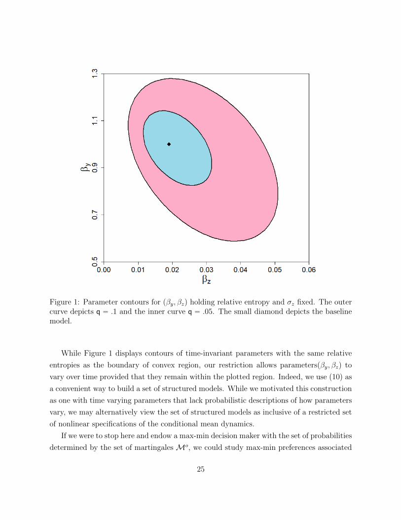
Figure 1: Parameter contours for pβy, βzq holding relative entropy and σz fixed. The outercurve depicts q “ .1 and the inner curve q “ .05. The small diamond depicts the baselinemodel.

While Figure 1 displays contours of time-invariant parameters with the same relative

entropies as the boundary of convex region, our restriction allows parameterspβy, βzq to

vary over time provided that they remain within the plotted region. Indeed, we use (10) as

a convenient way to build a set of structured models. While we motivated this construction

as one with time varying parameters that lack probabilistic descriptions of how parameters

vary, we may alternatively view the set of structured models as inclusive of a restricted set

of nonlinear specifications of the conditional mean dynamics.

If we were to stop here and endow a max-min decision maker with the set of probabilities

determined by the set of martingales Mo, we could study max-min preferences associated

25

with this set of probabilities. Restriction (10) on the set of Mo martingales guarantees

that the set of probabilities is rectangular and that therefore these preferences satisfy

the dynamic consistency axiom of Epstein and Schneider (2003) that justifies dynamic

programming. However, as we emphasize in section 6, our decision maker expands the set

of models because he wants to evaluate outcomes under probability models inside relative

entropy neighborhoods of structured models. This expanded set is not rectangular and for

reasons stated formally in subsection 8.2 can’t be made rectangular by following Epstein and

Schneider’s expansion procedure and still yield a set of models that will interest a decision

maker who like ours wants to apply Good’s plausibility criterion. But our decision maker

wants decisions that are robust to misspecifications that reside within a vast collection of

unstructured models that fit nearly as well as the structured models in Mo. That motivates

us to include unstructured models while using a penalty to limit their entropies relative to

the family of structured models in Mo. Before describing how we do this in section 6, we

briefly describe approaches suggested by other authors.

5.5 Other approaches

In our example so far, we have assumed that the structured model probabilities can be

represented as martingales with respect to a baseline model. A different approach, invented

by Peng (2004), uses a theory of backward stochastic differential equations under a notion

of ambiguity that is rich enough to allow for uncertainty about conditional volatilities of

Brownian increments.20 Because alternative probability specifications fail to be absolutely

continuous (over finite time intervals), standard likelihood ratio analysis does not apply.

This approach would push us outside the Chen and Epstein (2002) formulation but would

still let us construct a rectangular embedding that we could use to construct structured

models. Epstein and Ji (2014) applied the Peng approach to asset pricing.

6 Including unstructured alternatives

In section 5.1, we described how the decision maker forms a set Mo of structured models

that are parametric alternatives to the baseline model. To represent the unstructured

models that also concern the decision maker, we proceed as follows. After constructing

20See Chen et al. (2005) for a further discussion of Peng’s characterizations of a class of nonlinearexpectations to Choquet integration used in decision theory in both economics and statistics.

26

Mo, for scalar ξ ą 0, we define a scaled discrepancy of martingale MU from a set of

martingales Mo as

ΞpMU|F0q “ ξ inf

MSPMo∆`

MU ;MS|F0

˘

“ξδ

2

ż 8

0

expp´δtqE”

MUt γtpUtq

ˇ

ˇ

ˇF0

ı

dt. (28)

where

γtpUtq “ infStPΓt

|Ut ´ St|2. (29)

Scaled discrepancy ΞpMU |F0q equals zero for MU in Mo and is positive for MU not in Mo.

We use discrepancy ΞpMU |F0q to define a set of unstructured models near Mo whose utility

consequences a decision maker wants to know. When we pose a max-min decision problem,

we use the scaling parameter ξ to measure how the expected utility minimizer is penalized

for choosing unstructured models that are statistically farther from the structured models

in Mo.

The decision maker doesn’t stop with the set of structured models generated by martin-

gales in Mo because he wants to evaluate the utility consequences not just of the structured

models in Mo but also of unstructured models that statistically are difficult to distin-

guish from them. For that purpose, he employs the scaled statistical discrepancy measure

ΞpMU |F0q defined in (28).21

7 Recursive Representation of Preferences

The decision maker uses relative entropy implied by the scaling parameter ξ to restrain

statistical discrepancies between unstructured models and the set of structured models. In

particular, the decision maker solves a minimization problem in which ξ serves as a penalty

parameter that effectively excludes unstructured probabilities that are statistically too far

from the set Mo of structured models. That minimization problem induces a special case

of the dynamic variational preference ordering that Maccheroni et al. (2006b) showed is

dynamically consistent.

21Watson and Holmes (2016) and Hansen and Marinacci (2016) discuss misspecification challenges con-fronted by statisticians and economists.

27

7.1 Continuation values

The decision maker ranks alternative consumption plans with a scalar continuation value

stochastic process. Date t continuation values reveal a decision maker’s date t ranking.

Continuation value processes have a recursive structure that makes preferences be dynam-

ically consistent. Thus, for Markovian plans, a Hamilton-Jacobi-Bellman (HJB) equation

restricts the evolution of continuation values. In particular, for a consumption plan tCtu,

a continuation value process tVtu8t“0 is defined by

Vt “ mintUτ :tďτă8u

E

ˆż 8

0

expp´δτq

ˆ

MUt`τ

MUt

˙„

ψpCt`τ q `

ˆ

ξδ

2

˙

γt`τ pUt`τ q

dτ | Ft

˙

(30)

where ψ is an instantaneous utility function. We can use (30) to derive an inequality that

describes a sense in which a minimizing process tUτ : t ď τ ă 8u isolates a statistical model

that is robust. After deriving and discussing this inequality and the associated robustness

bound, we shall use (30) to provide a recursive representation of preferences.

Turning to the derived bound, we proceed by applying an inequality familiar from

optimization problems subject to penalties. Let U o be the minimizer for problem (30) and

let So “ SpU oq be the minimizing S implied by equation (29). The process affiliated with

the pair pU o, Soq gives a lower bound on discounted expected utility that can be represented

in the following way.

Bound 7.1. If pU, Sq satisfies:

δ

2E

ˆż 8

0

expp´δτq

ˆ

MUt`τ

MUt

˙

|St`τ ´ Ut`τ |2dτ | Ft

˙

ďδ

2E

ˆż 8

0

expp´δτq

ˆ

MUo

t`τ

MUot

˙

|Sot`τ ´ Uot`τ |

2dτ | Ft

˙

(31)

then

E

ˆż 8

0

expp´δτq

ˆ

MUt`τ

MUt

˙

ψpCt`τ qdτ | Ft

˙

ě E

ˆż 8

0

expp´δτq

ˆ

MUo

t`τ

MUot

˙

ψpCt`τ qdτ | Ft

˙

(32)

for all t ě 0.

Inequality (32) is a direct implication of minimization problem (30). It gives probability

28

specifications that have date t discounted expected utilities that are at least as large as the

one parameterized by U o. The structured models all satisfy this bound; so do unstructured

models that are statistically close to them as measured by the date t conditional counterpart

to our discrepancy measure.

Turning next to a recursive representation of preferences, note that equation (30) implies

that

Vt “ mintUτ :tďτăt`εu

"

E

„ż ε

0

expp´δτq

ˆ

MUt`τ

MUt

˙„

ψpCt`τ q `

ˆ

ξδ

2

˙

γt`τ pUt`τ q

dτ | Ft

` expp´δεqE

„ˆ

MUt`ε

MUt

˙

Vt`ε | Ft

*

(33)

for ε ą 0. Heuristically, we can “differentiate” the right-hand side of (33) with respect to ε

to obtain an instantaneous counterpart to a Bellman equation. Viewing the continuation

value process tVtu as an Ito process, write:

dVt “ νtdt` ςt ¨ dWt.

A local counterpart to (33) is then

0 “ minUt

„

ψpCtq ´ξδ

2γtpUtq ´ δVt ` Ut ¨ ςt ` νt

“ minStPΓt

minUt

„

ψpCtq `ξδ

2|Ut ´ St|

2´ δVt ` Ut ¨ ςt ` νt

“ minStPΓt

„

ψpCtq ´1

2ξδςt ¨ ςt ´ δVt ` St ¨ ςt ` νt

(34)

where the minimizing Ut expressed as a function of St satisfies

Ut “ St ´1

δξςt

The term Ut¨ςt on the right side of (34) comes from an Ito adjustment to the local covariance

betweendMU

t

MUt

and dVt. Equivalently, Ut ¨ ςt is an adjustment to the drift νt of dVt that is

induced by using martingale MU to change the probability measure. For a continuous-time

Markov decision problem, (34) gives rise to an HJB equation for a corresponding value

function expressed as a function of a Markov state.

Remark 7.2. With preferences described by (34), we can still discuss admissibility relative

29

to a set of structured models using the representation on the third line of (34). Recall that

the S process parameterizes a structured model. For a given decision process C, solve

0 “ ψpCtq ´1

2ξδςt ¨ ςt ´ δVt ` St ¨ ςt ` νt

where

drV “ νtdt` ςt ¨ dWt.

Solving this equation backwards for alternative C processes gives a ranking of them for a

given S probability. By posing a Markov decision problem, we can study admissibility by

applying a Minimax theorem along with a Bellman-Isaacs condition for a dynamic two-

person game. See, for instance, Fleming and Souganidis (1989). If we can exchange orders

of maximization and minimization, then the implied worst-case structured model process S˚

can be used in the fashion recommended by Good (1952) in the quote with which we began

this paper.

By extending Bound 7.1, the implied adjustment U˚ for misspecification of the struc-

tured models is also enlightening. Specifically, we can use pU˚, S˚q in place of pU o, Soq in

inequality (31) and conclude that a counterpart to inequality (32) holds in which we maxi-

mize both the right and left sides by choice of a C plan subject to the constraints imposed on

the decision problem. Thus, the entropy of U˚ relative to S˚ tells us over what probabilities

we can bound discounted expected utilities.

Remark 7.3. It is useful to compare roles of the baseline model here and in the robust de-

cision model based on the multiplier preferences of Hansen and Sargent (2001) and Hansen

et al. (2006), another continuous time version of variational preferences.22 Their baseline

model is a unique structured model, distrust of which motivates a decision maker to com-

pute a worst-case unstructured model to guide evaluations and decisions. In the present

paper, the baseline model is just one of a set of structured models that the decision maker

maintains. The baseline model here merely anchors specifications of other members of the

set of structured models. The decision maker in this paper distrusts all models in the set of

22Our way of formulating preferences differs from how equation (17) of Maccheroni et al. (2006b) describesHansen and Sargent (2001) and Hansen et al. (2006)’s “multiplier preferences”. The disparity reflects whatwe regard as a minor blemish in Maccheroni et al. (2006b). The term ξδ

2 γt in our analysis is γt in Maccheroniet al. (2006b) and our equation (34) is a continuous time counterpart to equation (12) in their paper. InHansen and Sargent (2001) and Hansen et al. (2006), γt “ |Ut|

2 as we define γt. We point out this minorerror here only because the analysis in the present paper generalizes our earlier work by now measuringdiscrepancy from a non-singleton set Mo of structured models rather than from a single structured model.

30

structured models associated with martingales in Mo.

8 Relative entropy versus rectangularity

This section is dedicated to showing how using relative entropy (without our refinement) to

constrain a set of alternative models can result in an extremely large rectangular embedding

that contains very implausible models. Subsection 8.1 uses a simple two-period model to

display the basic idea while section 8.2 employs the continuous-time Brownian information

structure that we use throughout the rest of this paper.

8.1 Anything goes: take 1

In this subsection, time takes values 0, 1, 2. At time t “ 2, one of J states can be realized

that we denote j “ 1, ..., J. We represent information available at date t “ 1 by a size I ď J

partition Λi, i “ 1, 2, ..., I of the collection of the J states. Every state j is contained in

exactly one Λi.

Let πi ą 0 denote the baseline probability of Λi, and let πi pPi,j ą 0 denote the baseline

probability assigned to j in Λi. Thus, pPi,j is the baseline conditional probability of state j

given partition i. Similarly, we use πiPi,j to represent alternative probabilities assigned to

Λi. From the point of view of time 0, the entropy of an alternative probability relative to

the baseline probability is

ε0.“

Iÿ

i“1

ÿ

jPΛi

πiPi,j

´

logPi,j ` log πi ´ log pPi,j ´ log πi

¯

“

Iÿ

i“1

πi pε1,i ` log πi ´ log πiq . (35)

where

ε1,i “ÿ

jPΛi

Pi,j

´

logPi,j ´ log pPi,j

¯

Expression (35) represents joint entropy ε0 in terms of a sum of an expected value of

“continuation conditional relative entropies” ε1,i of the time t “ 2 possible outcomes and

the unconditional relative entropyřIi“1 πiplog πi ´ log πiq of the marginal distribution of

the time t “ 1. This is an example of what is sometimes called a “chain rule of relative

entropy.”

31

To relate this structure to positive martingales with mathematical expectations equal

to 1 that are used throughout this paper, let M2 denote a random variable that is equal

to the probability ratioπiPij

πi pPijin state j and let M1 equal the probability ratio πi

πiwhen

j P Λi. It can be verified under the baseline probability that the expectation M2 equals M1

conditional on information at t “ 1 and that the unconditional mathematical expectation

of M1 equals 1. Written in terms of M2 and M1, time 0 entropy is

ε0 “ E rM2 plogM2 ´ logM1qs ` E pM1 logM1q

“ E rM1 pε1 ` logM1qs (36)

where

ε1 “ E

„ˆ

M2

M1

˙

plogM2 ´ logM1q | F1

and F1 denotes the date one sigma algebra constructed from the partition. Versions of

formula (36) that are cast in terms of a mean 1 positive martingale tMtu extend to more

general probability specifications and to more time periods. In later sections of this paper,

we use a continuous-time limiting version of formula (36) that we modify to incorporate

discounting the future at a fixed discount rate.

We now show that a rectangular embedding of the baseline model imposes extremely

weak restrictions on the continuation entropies ε1,i. Represent relative entropy ε0 as

ε0 “ Hpπ, ε1q “Iÿ

i“1

πi pε1,i ` log πi ´ log πiq . (37)

We use the H notation to make explicit the dependence of ε0 on the vector π of probabilities

and the vector ε1 date t “ 1 continuation entropies. We impose the following restriction

on date 0 entropy

Hpπ, ε1q ď ε (38)

where ε ą 0. Inequality (38) is an ex ante constraint that jointly restricts pπ, ε1q as deter-

minants of time 0 relative entropy.

We want a set of probabilities surrounding the baseline probability that is rectangular

in the sense of Epstein and Schneider (2003), i.e., we want a “rectangular embedding of

a set of probabilities that is not rectangular.” To construct a rectangular embedding, we

shall seek the weakest restriction that (37) and (38) impose on ε1,` for a given ` as we search

over alternative vectors π of probabilities and vectors ε1 of continuation entropies.

32

We prove the following result in Appendix B

Claim 8.1. The rectangular embedding is described by:

ε1,` ď sup0ăπ`ď1

ε´ p1´ π`q rlogp1´ π`q ´ logp1´ π`qs ´ π` plog π` ´ log π`q

π`. (39)

for ` “ 1, 2, ...I.

Sometimes the right-hand side of (39) can be made arbitrarily large by letting π` de-

crease to zero. To discover when, note that

limπ`Ó0

π`plog π` ´ log π`q “ 0

limπ`Ó0

p1´ π`q rlog p1´ π`q ´ log p1´ π`qs “ ´ log p1´ π`q

Therefore, as π` Ñ 0 the numerator of the right-hand side of inequality (39) approaches

ε` log p1´ π`q

It is convenient to construct the threshold

π.“ 1´ exp p´εq

that satisfies

ε` log p1´ πq “ 0.

If π` ă π, the numerator of the right side of inequality (39) remains strictly positive as π`

converges to zero. But the denominator of the right side of inequality (39) converges to

zero as π` converges to zero, implying that the ratio diverges to plus infinity.

Corollary 8.2. If π` ă π, then the rectangular embedding does not restrict ε`. Furthermore,

if π` ă π for all `, the rectangular embedding does not restrict any ε1,`.

Figure 2 plots the right-hand side of inequality (39) as a function of π` for two cases,

one in which π` ą π and a second in which π` ă π. In the first large π` case, an interior

maximum occurs to the left of π. In the second small π` case, the function is unbounded as

π` tends to zero. In the second low-baseline-probability case, by adopting a rectangular em-

bedding, we relax – indeed we completely eliminate – an upper bound on each continuation

entropy ε1,`.

33

0 0.2 0.4 0.6 0.8 1−8

−6

−4

−2

0

0 0.2 0.4 0.6 0.8 1−4

−2

0

2

4

6

8

Figure 2: Entropy bounds implied by a rectangular embedding as described by the right-hand side of inequality (39) as a function of π` for two cases. The maxima equal the inducedbounds on continuation entropies. When η “ 0.05, the threshold is π “ 0.049. The leftpanel imposes π` “ 0.1, and the right panel assumes π` “ 0.025. Vertical lines depictπ` “ π`.

Although we do not prove it here, corollary 8.2 suggests an analogue for a continuous

baseline probability distribution for which a counterpart to the π` ă π would automatically

be satisfied.

8.2 Anything goes: take 2

In this subsection, we show that if a decision maker starts with a set of unstructured models

constrained by relative entropy to be close to the set of structured models, enlarging that

set to make it rectangular results in the set of all unstructured models that are absolutely

continuous to a structured model over finite intervals. Most of those are statistically very

implausible and not ones that the decision maker is concerned about.

Our decision maker starts with a set of structured probability models that we have con-

structed to be rectangular in the sense of Epstein and Schneider. But our decision maker’s

suspicion that all of these structured models are misspecified motivates him to explore the

utility consequences of a larger set that includes unstructured probability models. This

larger set is not rectangular, even though as measured by relative entropy, all of the un-

structured models are statistically close to models in the rectangular set formed by the

structured models.

34

An alternative to formulating the decision maker’s problems with the dynamic varia-

tional preferences of Maccheroni et al. (2006b) would have been first to construct a set that

includes relative entropy neighborhoods of all martingales in Mo. For instance, for ε ą 0,

Ξ given by (28), and ξ “ 1, we could have started with a set

M “

MUPM : ΞpMU

|F0q ă ε(

. (40)

The set of implied probabilities is not rectangular. At this point, why not follow Epstein and

Schneider’s (2003) recommendation and add just enough martingales to attain a rectangular

set of probability measures? A compelling practical reason not to do so is that doing so

would include all martingales in M defined in definition 3.1 – implying a set much too

large for an interesting max-min decision analysis.

To show this, it suffices to look at relative entropy neighborhoods of the baseline model.23

To construct a rectangular set of models that includes the baseline model, for a fixed date

τ , consider a random vector U τ that is observable at τ and that satisfies

E`

|U τ |2| F0

˘

ă 8.

Form a stochastic process

Uht “

$

’

&

’

%

0, 0 ď t ă τ

U τ , τ ď t ă τ ` h

0, t ě τ ` h.

The martingale MUh associated with Uh equals one both before time τ , and MUh

t {MUh

h`τ

equals one after time h` τ . Compute relative entropy:

∆pMUh|F0q “

ˆ

1

2

˙ż τ`h

τ

expp´δtqE”

MUh

t |U τ |2dt

ˇ

ˇ

ˇF0

ı

dt

“

„

1´ expp´δhq

2δ

expp´δτqE`

|U τ |2| F0

˘

.

Evidently, relative entropy ∆pMUh |F0q can be made arbitrarily small by shrinking h to zero.

This means that any rectangular set that contains M must allow for a drift distortion U τ

at date τ . This argument implies the following proposition:

Proposition 8.3. Any rectangular set of probabilities that contains the probabilities induced

23Including additional structured models would only make the set of martingales larger.

35

by martingales in M must also contain the probabilities induced by any martingale in M.

This rectangular set of martingales allows too much freedom in setting date τ and

random vector U τ : all martingales in the set M isolated in definition 3.1 are included in

the smallest rectangular set that embeds the set described by (40). That set is too big to

pose a max-min problem for a decision maker who wants to apply the plausibility check

recommended by Good (1952).

9 Conclusion

While important aspects of our analysis apply in more general settings, we have added

inessential auxiliary assumptions that we find enlightening and that set the stage for con-

crete applications. Extensions of the framework presented here would relax the Brownian

information structure and would not use relative entropy to constrain a family of structured

models. Our continuous-time formulation (34) exploits mathematically convenient prop-

erties of a Brownian information structure. A discrete-time version starts from a baseline

model cast in terms of a nonlinear stochastic difference equation. Counterparts to struc-

tured and unstructured models play the same roles that they do in the continuous time

formulation described in this paper. In the discrete time formulation, preference orderings

defined in terms of recursions on continuation values are dynamically consistent.

In both continuous time and discrete time settings, there are compelling reasons for a

decision maker to think that a rectangular set of structured probability models does not

describe the set of probabilities that concerns him. The set of structured models is too small

because it excludes interesting statistically nearby unstructured models. But a rectangular

embedding of unstructured probabilities of concern to the decision maker models is too

large because it includes models that are statistically very implausible in the sense of Good

(1952). Therefore, the decision maker uses the framework of the present paper to include

concerns about unstructured models that satisfy a penalty on entropy relative to the set of

structured models, the same type of statistical neighborhood routinely applied to construct

probability approximations in computational information geometry.24

A purpose of this paper is to provide a framework for analyzing the consequences of

long-term variations in macroeconomic growth coming from rates of technological progress,

climate change, and demographics that concern private and public decision makers in situa-

24See Amari (2016) and Nielsen (2014).

36

tions that naturally involve both ambiguity and misspecification fears as we have formalized

those concepts here.

While we do not explore the issue here, we suspect that the tension between admissibility

and dynamic consistency described in this paper is also present in other approaches to

ambiguity and misspecification, including ones proposed by Hansen and Sargent (2007)

and Hansen and Miao (2018).

37

Appendices

A Computing relative entropy

We show how to compute relative entropies for parametric models of the form (26). Recall

that relative entropy q2

2emerges as part of the solution to the second-order differential

equation (16) appropriately specialized to become:

|ηopzq|2

2`dρo

dzpzqr´pβzpz ´ zq ` σz ¨ ηpzqs `

|σz|2

2

d2ρ0

dz2pzq ´

q2

2“ 0.

where z “ pαzpβz

and

ηopzq “ η0 ` η1pz ´ zq.

Under our parametric alternatives, the solution for ρo is quadratic in z ´ z:

ρopzq “ ρ1pz ´ zq `1

2ρ2pz ´ zq

2.

Compute ρ2 by targeting only terms that involve pz ´ zq2:

η1 ¨ η1

2` ρ2

”

´pβz ` σz ¨ η1

ı

“ 0.

Thus,

ρ2 “η1 ¨ η1

2´

pβz ´ σz ¨ η1

¯ .

Given ρ2, compute ρ1 by targeting only the terms in pz ´ zq:

η0 ¨ η1 ` ρ2 pσz ¨ η0q ` ρ1

´

´pβz ` σz ¨ η1

¯

“ 0.

Thus,

ρ1 “η0 ¨ η1

pβz ´ σz ¨ η1

`pη1 ¨ η1q pσz ¨ η0q

2´

pβz ´ σz ¨ η1

¯2 .

Finally, calculate q by targeting the remaining constant terms:

η0 ¨ η0

2` ρ1 pσz ¨ η0q ` ρ2

|σz|2

2´

q2

2“ 0.

38

Thus,25

q2

2“η0 ¨ η0

2`η0 ¨ η1 pσz ¨ η0q

pβz ´ σz ¨ η1

`η1 ¨ η1 pσz ¨ η0q

2

2´

pβz ´ σz ¨ η1

¯2 `η1 ¨ η1|σz|

2

4´

pβz ´ σz ¨ η1

¯ .

B Proof of Claim 8.1

Proof. We begin by deducing a bound under the restriction π “ π, so that there are no

distortions of time t “ 1 probabilities. To obtain the weakest bound under this restriction,

we set ε1,i “ 0 for all i except for state `. Then

Hpπ, ε1q “ π`ε1,`

and constraint (38) implies that

ε1,` ďε

π`. (41)

Repeating this calculation for each ` “ 1, ..., I gives us a restricted set of continuation

entropies ε1 and is an example of a “rectangular restriction” on the date t “ 2 conditional

probabilities expressed in terms continuation entropies. Suppose that we now set each of

these continuation entropies at its upper bound. Then entropy ε0 is

Iÿ

`“1

π`ε1,` “ εI,

verifying that we have substantially expanded the set of admissible continuation entropies.

For a fixed ε, constraint (41) for each ` becomes weaker and weaker as we reduce probability

π` assigned to partition component Λ`.

We can loosen restriction (41) further by allowing πi ‰ πi and in particular by setting

π` ă π`. It is convenient to proceed in two steps. First, for a given pε1,`, π`q, minimize

Hpπ, ε1q by choosing pε1,i, πiq for i ‰ `. Evidently, the minimizers are ε1,i “ 0 for i ‰ `. It

is straightforward to show that the minimizing πi’s are proportional to the corresponding

πi’s and hence that for i ‰ `,

πi “p1´ π`qπi

1´ π`.

25We could also have derived this same formula by computing the expectation of |rηpZtq|2

2 under theperturbed distribution.

39

Notice that the proportionality coefficients 1´π`1´π`

guarantee that the altered probabilities

sum to 1:Iÿ

i“1

πi “ π` ` p1´ π`q “ 1.

Imposing these minimizing choices gives

H˚pπ, ε1,`q “Iÿ

i“1

πi pε1,i ` log πi ´ log πiq

“ π`pε1,` ` log π` ´ log π`q `

ˆ

1´ π`1´ π`

˙

rlogp1´ π`q ´ logp1´ π`qsÿ

i‰`

πi

“ π`pε1,` ` log π` ´ log π`q ` p1´ π`q rlogp1´ π`q ´ logp1´ π`qs

At these minimizing choices, entropy constraint (36) becomes

π`ε1,` ` π`plog π` ´ log π`q ` p1´ π`q rlogp1´ π`q ´ logp1´ π`qs ď ε.

40

References

Amari, Shu-nichi. 2016. Information Geometry and its Applications. Japan: Springer.

Anderson, Evan W., Lars Peter Hansen, and Thomas J. Sargent. 1998. Risk and Robustness

in General Equilibrium. Available on webpages.

Anderson, Evan W., Lars P. Hansen, and Thomas J. Sargent. 2003. A Quartet of Semi-

groups for Model Specification, Robustness, Prices of Risk, and Model Detection. Journal

of the European Economic Association 1 (1):68–123.

Barillas, Francisco, Lars P. Hansen, and Thomas J. Sargent. 2009. Doubts or Variability?

Journal of Economic Theory 144 (6):2388–2418.

Box, Goerge E. P. 1979. Robustness in the Strategy of Scientific Model Building. In

Robustness in Statistics, edited by Robert L. Launer and Graham N. Wilkinson, 201–

236. New York: Academic Press.

Chen, Zengjing and Larry Epstein. 2002. Ambiguity, Risk, and Asset Returns in Continuous

Time. Econometrica 70 (4):1403–1443.

Chen, Zengjing, Tao Chen, and Matt Davison. 2005. Choquet Expectation and Peng’s g

-expectation. Ann. Probab. 33 (3):1179–1199.

Epstein, Larry G. and Shaolin Ji. 2014. Ambiguous Volatility, Possibility and Utility in

Continuous Time. Journal of Mathematical Economics 50:269–282.

Epstein, Larry G. and Martin Schneider. 2003. Recursive Multiple-Priors. Journal of

Economic Theory 113 (1):1–31.

Fan, K. 1952. Fixed-point and Minimax Theorems in Locally Convex Topological Linear

Spaces. Proceedings of the National Academy of Sciences 38 (2):121–126.

Fleming, Wendell H. and Panagiotis E. Souganidis. 1989. On the Existence of Value Func-

tions of Two Player, Zero-sum Stochastic Differential Games. Indiana Univesity Mathe-

matics Journal 38:293–314.

Geweke, John and Gianni Amisano. 2011. Optimal prediction pools. Journal of Economet-

rics 164 (1):130–141.

41

Gilboa, Itzhak and David Schmeidler. 1989. Maxmin Expected Utility with Non-unique

Prior. Journal of Mathematical Economics 18 (2):141–153.

———. 2001. A Theory of Case-based Decisions. Cambridge University Press.

Good, Irving J. 1952. Rational Decisions. Journal of the Royal Statistical Society. Series

B (Methodological) 14 (1):pp. 107–114.

Hansen, Lars P. 2007. Beliefs, Doubts and Learning: Valuing Macroeconomic Risk. Amer-

ican Economic Review 97 (2):1–30.

Hansen, Lars P. and Thomas J. Sargent. 2010. Fragile Beliefs and the Price of Uncertainty.

Quantitative Economics 1 (1):129–162.

Hansen, Lars Peter. 2012. Dynamic Valuation Decomposition Within Stochastic Economies.

Econometrica 80 (3):911–967.

———. 2014. Nobel Lecture: Uncertainty Outside and Inside Economic Models. Journal

of Political Economy 122 (5):945–987.

Hansen, Lars Peter and Massimo Marinacci. 2016. Ambiguity Aversion and Model Mis-

specification: An Economic Perspective. Statistical Science 31 (4):511–515.

Hansen, Lars Peter and Jianjun Miao. 2018. Aversion to Ambiguity and Model Misspec-

ification in Dynamic Stochastic Environments. Proceedings of the National Academy of

Sciences 115 (37):9163–9168.

Hansen, Lars Peter and Thomas J. Sargent. 2001. Robust Control and Model Uncertainty.

American Economic Review 91 (2):60–66.

———. 2007. Recursive Robust Estimation and Control without Commitment. Journal of

Economic Theory 136 (1):1–27.

———. 2020. Macroeconomic Uncertainty Prices when Beliefs are Tenuous. Journal of

Econometrics forthcoming.

Hansen, Lars Peter, Thomas J. Sargent, and Thomas D. Tallarini. 1999. Robust Permanent

Income and Pricing. Review of Economic Studies 66 (4):873–907.

42

Hansen, Lars Peter, Thomas J. Sargent, Gauhar A. Turmuhambetova, and Noah Williams.

2006. Robust Control and Model Misspecification. Journal of Economic Theory

128 (1):45–90.

Hansen, Lars Peter, Balint Szoke, Lloyd S. Han, and Thomas J. Sargent. 2020. Twisted

probabilities, uncertainty, and prices. Journal of Econometrics 216:151–174.

James, Matthew R. 1992. Asymptotic Analysis of Nonlinear Stochastic Risk-Sensitive

Control and Differential Games. Mathematics of Control, Signals and Systems 5 (4):401–

417.

Klibanoff, Peter, Massimo Marinacci, and Sujoy Mukerji. 2009. Recursive Smooth Ambi-

guity Preferences. Journal of Economic Theory 144 (3):930–976.

Maccheroni, Fabio, Massimo Marinacci, and Aldo Rustichini. 2006a. Ambiguity Aver-

sion, Robustness, and the Variational Representation of Preferences. Econometrica

74 (6):1447–1498.

———. 2006b. Dynamic Variational Preferences. Journal of Economic Theory 128 (1):4–

44.

Nielsen, Frank. 2014. Geometric Theory of Information. Heidelberg and New York:

Springer.

Peng, Shige. 2004. Nonlinear Expectations, Nonlinear Evaluations and Risk Measures.

Stochastic Methods in Finance: Lectures given at the C.I.M.E.-E.M.S. Summer School

held in Bressanone/Brixen, Italy, July 6-12, 2003. Berlin, Heidelberg: Springer Berlin

Heidelberg.

Petersen, Ian R., Matthew .R. James, and Paul Dupuis. 2000. Minimax Optimal Control

of Stochastic Uncertain Systems with Relative Entropy Constraints. Automatic Control,

IEEE Transactions on 45 (3):398–412.

Sarin, Rakesh and Peter P. Wakker. 1998. Dynamic Choice and NonExpected Utility.

Journal of Risk and Uncertainty 17 (2):87–120.

Szoke, Balint. 2020. Estimating Robustness.

Waggoner, Daniel F. and Tao Zha. 2012. Confronting Model Misspecification in Macroe-

conomics. Journal of Econometrics 171 (2):167–184.

43

Wald, Abraham. 1950. Statisical Decision Functions. New York: John Wiley and Sons.

Watson, James and Chris Holmes. 2016. Approximate Models and Robust Decisons. Sta-

tistical Science 31 (4):465–489.

44