Asymptotic Properties of the

Maximum Likelihood Estimator in

Dichotomous Logistic Regression Models

Diploma Thesis

submitted to the

Department of MathematicsFaculty of SciencesUniversity of Fribourg Switzerland

in partial fulfilment of the requirementsfor the attainment of the

Diploma in Mathematics

by

Michael Beer

? ? ?

Academic supervisor: Prof Dr Andre AntilleSubmission date: December 2001

Address of the author: Henzenmoos 41, 3182 Uberstorf, SwitzerlandE-mail: Michael.Beer@unifr.ch

Abstract

This diploma thesis investigates the consistency and asymptotic normality ofthe maximum likelihood estimator in dichotomous logistic regression mod-els. The consistency is proved under hypotheses which allow the number ofexogenous variables p to grow along with the sample size n. Conditions onthe interdependence of p and n necessary for the consistency of the estima-tor are established. The asymptotic normality is proved in the case wherep is constant. Some aspects on the motivation and the origins of the modelare presented at the beginning. Finally, a short example based on a medicalstudy outlines the application of the logistic regression model.

Contents

1 Introduction 2

2 Logistic Regression Model 42.1 Model Specification . . . . . . . . . . . . . . . . . . . . . . . . 42.2 Maximum Likelihood Estimation of the Parameter β . . . . . 52.3 Motivation and Interpretation . . . . . . . . . . . . . . . . . . 82.4 History . . . . . . . . . . . . . . . . . . . . . . . . . . . . . . 13

3 Consistency 153.1 A Different Approach . . . . . . . . . . . . . . . . . . . . . . 153.2 Condition on the Relationship between p and n . . . . . . . . 223.3 Reformulation, Assessment, and Comparison . . . . . . . . . 23

4 Asymptotic Normality 27

5 Case Study 32

6 Conclusion 35

Acknowledgements 36

References 37

1

1 Introduction: A Regression Model for Dichoto-

mous Outcome Variables

Among the different regression models, logistic regression plays a particularrole. The base concept, however, is universal. In a statistical investigation,several variables are defined and their values are determined for a set ofobjects. Some of these variables are a priori considered to be dependenton others within the same framework. Others are thought to be exclusivelydependent on exterior and not quantified (or not quantifiable) aspects, butnot on further variables inside the same model. The main aim of a regressionanalysis is to reveal and specify the impact of the so-called independent orexogenous explanatory variables on the dependent or endogenous response.

The prevalent linear regression model is – under certain hypotheses – inmany circumstances a valuable tool for quantifying the effects of severalexogenous on one dependent continuous variable. For situations where thedependent variable is qualitative, however, other methods had to be devel-oped. One of these is the logistic regression model which specifically coversthe case of a binary (dichotomous) response.

In a first section of this thesis, the logistic regression model as well as themaximum likelihood procedure for the estimation of its parameters are in-troduced in detail. A notation is fixed and will be used throughout theremaining parts of this document. Furthermore, several ideas on the moti-vation of the model and the interpretation of its parameters are outlined.At the end, a short paragraph illuminates a few historical aspects in relationto the development of this model.

The second part examines the consistency of the maximum likelihood esti-mator for the model parameters. It will be shown that, if certain hypothesesare satisfied, this estimator converges in probability to the true parametervalues as the sample size increases. As a peculiarity of the procedure pre-sented in this thesis, the number of explanatory variables is allowed to growsimultaneously with the number of observations. Conditions on the admis-sible interdependence of both of these characteristics are given in order toensure the consistency of the estimator. Finally, these conditions are com-pared to the assumptions of an existing consistency theorem.

As another important property, the asymptotic normality of the estimatorbeing discussed is proved in section 4. Picking up the thread of the previouspart, this aspect is established in a similar context. In contrast to the proofof consistency, however, this section will be based on the “classical” approachwhere the number of independent variables is held constant.

To conclude, a short example attempts to illustrate the application of the lo-gistic regression model. Proceeding from a survey of health enhancing phys-

2

ical activity carried out by the Swiss Federal Offices of Sports and Statistics,an estimation will be made what effects the linguistic background of a Swissinhabitant has on his or her daily or weekly physical activity. The resultsare presented along with the Mathematica1 code used for the calculations.

1Mathematica is a registered trademark of Wolfram Research, Inc.

3

2 Logistic Regression Model

2.1 Model Specification

We consider a binary random variable y having a Bernoulli distribution,

yL∼ B

(1, π(x)

),

i.e. the variable y takes either the value 1 or the value 0 with probabilitiesπ(x) or 1 − π(x) respectively. x ∈ R

p is a vector of p exogenous variablesand π : R

p −→ [0, 1] a real-valued function. In fact, π(x) represents theconditional probability P (y = 1 |x) of y = 1, given x.

Let r := y − π(x), which allows us to rewrite our model as

y = π(x) + r ,

where r has an expectation of

E(r) = E(y − π(x)

)= E(y) − π(x) = π(x) − π(x) = 0 (2.1a)

and a variance of

Var(r) = Var(y) = π(x)(1 − π(x)

). (2.1b)

For the forthcoming analysis we are going to define the so-called logistictransformation σLR : R −→ [0, 1] by

σLR(z) :=exp z

1 + exp z=

1

1 + exp−z

which allows us to specify the probability function π as

π(x) := σLR(xTβ)

with a vector β ∈ Rp of unknown parameters. This specification yields the

logistic regression model with parameter β.

If we denote the inverse function of σLR, which is called logit transformation,by

logitπ = lnπ

1 − π,

we can write our regression model as

logitπ(x) = xTβ . (2.2)

4

-4 -2 2 4

0.2

0.4

0.6

0.8

1

PSfrag replacements

z

σLR(z)

σ′

LR(z)

-4 -2 2 4

0.05

0.1

0.15

0.2

0.25

PSfrag replacements

zσLR(z)

σ′

LR(z)

Figure 1: The logistic transformation σLR and its first derivative.

Furthermore, it will be important to note that

σ′LR(z) =∂

∂z

(exp z

1 + exp z

)

=(exp z)(1 + exp z) − (exp z)2

(1 + exp z)2

=exp z

(1 + exp z)2> 0 ∀ z ∈ R .

(2.3)

The shape of σLR and its first derivative σ′LR are displayed in figure 1.Possible motivations for this specific model shall be discussed in section 2.3.

2.2 Maximum Likelihood Estimation of the Parameter β

In order to estimate the true value β0 of the vector β = (β1, . . . , βp)T ∈ R

p,we consider a set of n observations {(yi,xi)}i∈{1,...,n} ∈

({0, 1} × R

p)n

ofmutually independent responses yi with respective explanatory variables xi

(i = 1, . . . , n). Assuming

yiL∼ B

(1, σLR(xT

i β0))

(i = 1, . . . , n) (2.4)

we consider the model

y = σLR(Xβ0) + r ,

5

where

y := (y1, y2, . . . , yn)T ∈ {0, 1}n ,

X :=

xT1...

xTn

∈ R

n×p , and

r := y − σLR(Xβ0) .

The function σLR applied to a vector z = (z1, . . . , zn)T ∈ Rn has to be

interpreted as σLR(z) := (σLR(z1), . . . , σLR(zn))T. By (2.1a) and (2.1b), weknow that

E(ri) = 0 (2.5a)

and

s2i := Var(ri) = σLR(xTi β0)

(1 − σLR(xT

i β0))

=exp xT

i β0

1 + exp xTi β0

· 1 + expxTi β0 − exp xT

i β0

1 + exp xTi β0

(2.5b)

=exp xT

i β0

(1 + exp xTi β0)2

= σ′LR(xTi β0) .

In this context, we shall analyse the maximum likelihood estimator β of thetrue parameter vector β0. The likelihood function is defined as

L(β) =n∏

i=1

P(y = yi)

=

n∏

i=1

(1

yi

)(σLR(xT

i β))yi(1 − σLR(xT

i β))1−yi

=n∏

i=1

(σLR(xT

i β)

1 − σLR(xTi β)

)yi (1 − σLR(xT

i β))

=n∏

i=1

exp(xT

i ˛)

1+exp(xT

i ˛)

1+exp(xT

i ˛)−exp(xT

i ˛)

1+exp(xT

i˛)

yi(

1 + exp(xTi β) − exp(xT

i β)

1 + exp(xTi β)

)

=n∏

i=1

(exp(xT

i β))yi

1 + exp(xTi β)

=n∏

i=1

exp(yi xTi β)

1 + exp(xTi β)

6

and yields the log-likelihood function

lnL(β) =n∑

i=1

ln(exp(yi xT

i β))−

n∑

i=1

ln(1 + exp(xT

i β))

= yTXβ −n∑

i=1

ln(1 + exp(xT

i β)).

(2.6)

To determine the maximum of this function, we consider the gradient

∇ lnL(β) = XTy −n∑

i=1

exp(xTi β)

1 + exp(xTi β)

︸ ︷︷ ︸

=σLR(xT

i˛)

xi = XTy − XTσLR(Xβ)

= XT (y − σLR(Xβ)) .

A necessary condition for β being the maximum likelihood estimator of β0

is therefore

XT(

y − σLR

(Xβ

))

= 0 . (2.7)

From the second partial derivatives

∂2

∂βs ∂βrlnL(β) =

∂

∂βs

(n∑

i=1

xir yi −n∑

i=1

xir σLR(xTi β)

)

= −n∑

i=1

xir∂

∂βsσLR(xT

i β) = −n∑

i=1

xir xis σ′LR(xT

i β)

we can derive the Hessian matrix Hln L(β) ∈ Rp×p of the log-likelihood

function lnL(β) given by

Hln L(β) = −XTD(β)X ,

where D(β) = (dij) ∈ Rn×n is a diagonal matrix defined by

dij =

{

σ′LR(xTi β) if i = j,

0 if i 6= j.(2.8)

Affirmation. Hln L(β) is negative semi-definite for any β ∈ Rp. �

Verification. We have

uT Hln L(β) u = −uTXTD(β)Xu = −n∑

i=1

(xTi u)2 σ′LR(xT

i β) . (2.9)

As the first derivative of σLR is always positive (see (2.3)), we can see fromequation (2.9) that uT Hln L(β) u ≤ 0 for all u ∈ R

p and all β ∈ Rp. ¨

7

We therefore know that, in any case, the log-likelihood function lnL(β)is concave. Consequently, any root of ∇ lnL(β) is a global maximum oflnL(β) and a maximum likelihood estimator of β0. The condition (2.7)therefore is not only necessary but also sufficient for β being a maximumlikelihood estimator of β0. However, neither its existence nor its uniquenessare a priori guaranteed.

Remark. If we assumed p ≤ n and rg X = p, we would obtain that Xu = 0is equivalent to u = 0, such that Hln L(β) were negative definite for allβ ∈ R

p and thus lnL(β) strictly concave. Any β satisfying condition (2.7)therefore would be the unique maximum likelihood estimator of β0. �

Even though the existence of β cannot be guaranteed for finite samplespaces, we shall prove in section 3 that the probability of non-existenceapproaches zero as n tends to infinity.

Iterative methods for obtaining the maximum likelihood estimator are pre-sented for example by Amemiya (1985, pp. 274-275).

2.3 Motivation and Interpretation

The logistic regression model is a common tool for handling dichotomousresponse variables. Several reasons account for this circumstance. We nowwant to focus on two of them: the interpretation of the regression parametersand the relationship with the logistic distribution. Other motivations, suchas the “formal connection of the logistic model with loglinear model theory”and “theoretical statistical considerations including the availability of ‘exact’analyses of individual parameters” mentioned by Santner and Duffy (1989,p. 206), shall not be investigated within the scope of this thesis.

2.3.1 Odds, Log Odds and the Odds Ratio

In order to discuss binary data and to interpret the regression coefficients,it is essential to mention the terms of odds and odds ratios as counterpartsto probabilities and probability ratios.

Suppose that an event A has a probability π. We then define the odds ofA as the probability that A occurs divided by the probability it does notoccur, i.e.

Odds(A) :=P (A)

P (Ac)=

π

1 − π, (2.10)

where Ac denotes the complementary event of A in the respective samplespace.

8

Such a way of thinking is quite common in practice. If in a sporting compe-tition, for example, the probability of one team winning is about 80 per-cent, many people say that the odds on this team winning are four toone. However, as Christensen (1997, p. 2) mentions, odds are not infre-quently confused with probabilities. In a document entitled “What Are theOdds of Dying?” the US National Safety Council (2001) states for instance:“The odds of dying from an injury in 1998 were 1 in 1,796.” This numberwas approximated by dividing the 1998 US population (270,248,000) by therespective number of deaths (150,445). From a statistical point of view,the number 1,796 is an estimation of the reciprocal probability, whereasan estimation of the real odds on dying from an injury would rather be150,445/(270,248,000 − 150,445), i.e. 1 to 1,795. The expression “1 in” in-stead of “1 to” and the large numbers involved in this study justify such anapproximation procedure to a certain extent.

This latter example points out the need of careful distinction between oddsand probability. Note however, that there is a one-to-one relationship be-tween both of them.2 Given the probability π, the respective odds o areobtained by formula (2.10), while π is calculated from any given o byπ = o/(1 + o). As Christensen (1997, p. 3) emphasises, examining oddstherefore amounts to a rescaling of the measure of uncertainty: Probabili-ties between 0 and 1/2 correspond to odds between 0 and 1 whereas oddsbetween 1 and ∞ correspond to probabilities between 1/2 and 1.

The loss of symmetry inherent in the transformation of probabilities to oddscan be offset by a subsequent application of the natural logarithm function.Looking at the so-called log odds, we observe that they are “symmetric aboutzero just as probabilities are symmetric about one half” (Christensen 1997,p. 3). This is why mathematical analyses often deal with log odds insteadof “simple” odds. It is worth noting that the log odds are usually allowed totake the values −∞ and +∞ in order to establish a one-to-one relationshipwith the respective probabilities 0 and 1, and, moreover, that the trans-formation of probabilities to log odds is exactly the logit transformationintroduced in section 2.1.

In order to compare the odds of two different events, it may be useful toexamine not only odds but also odds ratios. If the odds of an event A areOdds(A) and the odds of an event B are Odds(B), then the odds ratioof B to A is defined as Odds(A)

/Odds(B).3 In the above study on the

“Odds of Dying”, for instance, the odds of dying in a railway accident were1 to 524,752 whereas the odds of an accidential death in a motor-vehicle

2This holds under the condition that the odds are allowed to take the value +∞ whenthe probability π equals 1.

3Note that this syntax is not used identically throughout the literature. While manyauthors just speak of the ratio of the odds of A to the odds of B, Garson (2001, “Log-linearModels, Logit, and Probit”) explicitly refers to the expression “odds ratio of B to A”.

9

were 1 to 6,211. The odds ratio of dying in a railway accident to dying ina motor-vehicle in the USA thus was about 84, i.e. the odds of dying ina motor-vehicle were about 84 times as important as those of dying in arailway crash.

2.3.2 Interpretation of the Parameter β

For an interpretation of the parameter β, let x ∈ Rp and x := x + ei where

ei denotes the ith canonical base vector of Rp for an arbitrary i ∈ {1, . . . , p}.

A comparison of the two model equations (2.2) for x and x gives

logitπ(x) = xTβ

logitπ(x) = xTβ = (x + ei)Tβ = xTβ + eT

i β

from where we get the difference

logitπ(x) − logitπ(x) = eTi β = βi .

On the other hand,

logitπ(x) − logitπ(x) = ln

(π(x)

1 − π(x)

)

− ln

(π(x)

1 − π(x)

)

= ln

π(x)1−π(x)

π(x)1−π(x)

.

We thus see that expβi is the odds ratio of {y = 1} given x to {y = 1}given x. In other words, the odds on the event that y equals 1 increase (ordecrease) by the factor expβi if xi grows by one unit. If in a certain study,for example, β2 has an estimated value of about 0.693, a unit increase inx2 is likely to double the odds on getting a positive response (y = 1), asexp 0.693 ≈ 2.

According to Hosmer and Lemeshow (1989, p. 41), “this fact concerning theinterpretability of the coefficients is the fundamental reason why logistic re-gression has proven such a powerful analytic tool for epidemiologic research.”At least, this argumentation holds whenever the explanatory variables x arequantitative.

Collett (1991, pp. 242-246) gives an outline of a suitable procedure for thecase of qualitative exogenous variables. Assume, for instance, that the prob-ability π is to be related to a single exposure factor g that has m levels, ex-pressed through integer values between 0 and m− 1. Instead of introducingg into a model like

logitπ = β0 + β1 g ,

10

it is preferable to define a set of dummy variables x1, . . . , xm−1 as

xi :=

{

1 if g = i,

0 if g 6= i,(i = 1, . . . ,m− 1)

and to analyse the model

logitπ = β0 + β1 x1 + · · · + βm−1 xm−1

for instance. This procedure allows to distinguish between the effects on yof every single factor level of g. An application of this idea will be shown insection 5.

The possibility of interpreting the coefficients of β as logarithms of odds ra-tios provides the foundation of a second important motivation of the logisticmodel. Both Santner and Duffy (1989, pp. 206-207) and Christensen (1997,pp. 118-120, p. 387) emphasise on the difference between prospective andretrospective studies. Consider for instance an experiment in which 250 peo-ple of an arbitrary population are sampled. A binary response “diseased”(D) or “non-diseased” (Dc) is observed for each person. Moreover, there is asingle explanatory variable “exposed” (E) or “non-exposed” (Ec) involved.This kind of study is called prospective. Let ψP denote the (prospective)ratio of odds of disease for the exposed group to odds of disease for thenon-exposed group as

ψP =P (D|E)

1 − P (D|E)

/P (D|Ec)

1 − P (D|Ec).

According to the nature of the study, diseased individuals may be very rarein a random sample of 250 people. So most of the collected data is aboutnon-diseased persons. It is therefore sometimes useful to fix the sample sizein the rare event category by design. In our example, one could possiblystudy separated samples of 100 diseased and 150 non-diseased individualswhile determining for every person whether he or she had been exposed ornot. This procedure is called retrospective and leads directly to informationabout the probability of exposure among the diseased and among the healthygroups. We thus get the (retrospective) odds ratio

ψR =P (E|D)

1 − P (E|D)

/P (E|Dc)

1 − P (E|Dc).

However, we obtain by Bayes’s rule that

ψP =

P (D|E)P (Dc|E)

P (D|Ec)P (Dc|Ec)

=

P (E|D)P (D)P (E|Dc)P (Dc)

P (Ec|D)P (D)P (Ec|Dc)P (Dc)

=

P (E|D)P (E|Dc)

1−P (E|D)1−P (E|Dc)

= ψR

so that we are able to make inferences about ψP even from a retrospectivestudy. The generalisation of this result motivates the inspection of oddsratios.

11

2.3.3 Relationship with the Logistic Distribution

Another important issue in connection with the logistic model is outlinedby Amemiya (1985, pp. 269-270) and Cramer (1991, pp. 11-13). Both ofthem cite two examples, one a biometric threshold model and the other aneconometric utility model.

In the biometric model, they suppose a dosage xi of an insecticide is given tothe ith insect of a population. Furthermore, it is assumed that every insecthas its own tolerance or threshold level y∗i against this insecticide. If thedosage xi is higher than y∗i , the insect dies, if it is lower, the insect survives.The binary variable yi expresses whether the ith insect dies (yi = 1) or not(yi = 0). We thus get

P (yi = 1) = P (y∗i < xi) = F (xi) ,

where F is the cumulative distribution function of the random variable y∗i .

The econometric model, on the other hand, attributes separate random util-ities u1 and u0 to the two possible states y = 1 and y = 0 of a certain variabley. For example, y = 1 could express that a person drives a car whereas y = 0would mean that this person travels by transit to work. Both utilities u1

and u0 are assumed to depend on certain characteristics, represented by avector xi, as

ui = xTi β + εi (i = 0, 1) ,

where εi is a random error term. If we suppose that our individual maximisesits utility, the probability of his decision in favour of the state y = 1 istherefore given by

P (y = 1) = P (u0 < u1) = P (xT0 β + ε0 < xT

1 β + ε1)

= P (ε0 − ε1 < xT1 β − xT

0 β) = F((x1 − x0)

Tβ),

where F is the cumulative distribution function of the random variable ε :=ε0 − ε1.

In both of these examples, an assumption on the shape of the cumulativedistribution function F or rather on the distribution of the underlying ran-dom variable has to be made in order to estimate the probability of theevent {y = 1}. With respect to the central limit theorem, the assumptionF = Φ(0, 1), where the so-called probit function Φ(0, 1) is the cumulativedistribution function of the standardised normal distribution, could mostprobably be justified, at least after an appropriate standardisation of therelevant data. This specific choice would lead to what is called the probitmodel.

12

However, the logistic transformation σLR itself provides a very similar andanalytically sometimes more convenient alternative. Being viewed as a dis-tribution function, σLR gives rise to the logistic distribution. Its density σ′

LR

has mean zero and variance π2/3, so that it is appropriate to define the cu-mulative distribution function of the standardised logistic distribution withzero mean and unit variance as

Λ(x) := σLR(λx) =expλx

1 + expλx

where λ = π/√

3. In the literature, for example by Cramer (1991), thefunction Λ is sometimes called logit function and is therefore not to beconfused with the logit transformation introduced in section 2.1, which isnearly its inverse.

Cramer (1991, section 2.3) shows in an example that “by judicious adjust-ment of the linear transformations of the argument x, the logit and probitprobability functions can be made to coincide over a fairly wide range.”Moreover, he states that “logit and probit functions which have been fittedto the same data are therefore virtually indistinguishable, and it is impossi-ble to choose between the two on empirical grounds.”

As a result, it is justifiable in most cases to assume a logistic distributioninstead of a normal distribution for y∗i or ε in examples as those mentionedabove. This, however, guides us again to the logistic regression approach.

2.4 History of the Logistic Regression Model

An overview of the development of the logistic regression model is given byCramer (1991, section 2.9). He identifies three sources having lead to thismodel as it is known today: applied mathematics, experimental statistics,and economic theory.

While studying the development of the human population, Thomas RobertMalthus (1766-1834) described an increase “in geometric progression”. Itcan be argued that at the basis of this statement, there was the formula forexponential growth, N(t) = A expαt, evolving directly from the differentialequation N(t) = αN(t) where N(t) denotes the size of a population at atime t. This model, however, did not take into consideration the possibilityof a saturation in the growth process. For this reason, Pierre Francois Ver-hulst (1804-1849) added an upper limit or saturation value W to the equa-tion mentioned above: N(t) = βN(t)(W−N(t)). Defining Z(t) := N(t)/W ,we obtain an equation of the form Z(t) = γZ(t)(1−Z(t)) whose solution isthe logistic function

Z(t) =exp(α+ γt)

1 + exp(α+ γt).

13

As Cramer (1991) states, this model of human population growth was in-troduced independently of Verhulst’s study by Raymond Pearl and LowellReed in an article entitled “On the rate of growth of the population of theUnited States since 1790 and its mathematical representation” published in1920. Cramer continues: “The basic idea that growth is proportional bothto the level already attained and to the remaining room to the saturationceiling is simple and effective, and the logistic model is used to this day tomodel population growth or, in market research, to describe the diffusionor market penetration of a new product or of new technologies. For newcommodities that satisfy new needs like television, compact discs or videocameras, the growth of ownership is naturally proportional both to the pen-etration rate already achieved and to the size of the remaining potentialmarket, and similar arguments apply to the diffusion of new products andtechniques in industry.”

The application of probability models to biological experiments in the thir-ties of the twentieth century represents another foundation of the logisticregression model. However, it was in the first place the probit model intro-duced in section 2.3.3 which found its reflection in the literature. Accordingto Cramer, economists at that time did not seem to take the logit modelseriously. Only after Henri Theil 1969 generalised the bivariate or dichoto-mous to the multinomial logit model with more than two states of the de-pendent variable, the logistic regression gained its wide acceptance. In theseventies, Daniel McFadden, winner of the 2000 Nobel Prize in economics,and his collaborators finally provided a theoretical framework to the logitmodel linking it directly to the mathematical theory of economic choice (seeMcFadden 1974).

14

3 Consistency of the Maximum Likelihood Esti-

mator

3.1 A Different Approach

In this section, we are going to investigate the consistency of the maxi-mum likelihood estimator β. More precisely, we are going to show that β

converges under certain hypotheses to the real value β0 if the number nof observations (yi,xi) considered in the model tends to infinity. This, ofcourse, is a purely theoretical viewpoint since it will never be possible to in-clude an infinity of samples in an empirical statistical analysis. Nonetheless,the consistency of an estimator is an important aspect of its nature.

Different proofs of consistency can be found in the literature (see e.g. Gou-rieroux and Monfort (1981) or Amemiya (1985, pp. 270-274)). All of theminclude or base upon the fact that the probability of the existence of theestimator β approaches 1 as n tends to infinity. Furthermore, they proceedon the assumption that the number p of exogenous variables is fixed onceand for all. In other words, p is compelled to remain constant while thesample size n grows.

Results presented by Mazza and Antille (1998) shall enable us to release thislast aspect. We are going to assume that p is variable but dependent on nand to examine what relationship between p and n is necessary in order notto destroy the consistency of our estimator β. Intuition suggests that thenumber of observations should be larger than the number of real parametersto be estimated, i.e. n > p. The requirements on p, however, are more subtleas we will see on the following pages.

Following Mazza and Antille (1998), we now define the error function

Ey,σ(β) := 1Tn Hσ(Xβ) − yTXβ , (3.1)

where 1n := (1, . . . , 1)T ∈ Rn and Hσ is a primitive of σ : R −→ R. Consid-

ering the gradient

∇Ey,σ(β) = XTσ(Xβ) − XTy = XT(σ(Xβ) − y

)

we become aware that

∇ lnL(β) = −∇Ey,σLR(β) .

Any estimator β which maximises the log-likelihood function lnL minimisesthus simultaneously the error function Ey,σLR

. This, however, is not verysurprising. If we take into consideration that a possible primitive of σLR is

15

HσLR(z) = ln(1+exp z), we see directly by (2.6) and (3.1) that Ey,σLR

(β) =− lnL(β).

The theorem 1 provided by Mazza and Antille (1998, p. 4) based on thedefinition of Ey,σ is therefore directly applicable to our logistic regressionmodel. On the following pages, we shall recite this theorem and its proof ina variant slightly adjusted to our problem.4

Assumptions. We consider the following assumptions:

M1:∑p

j=1

∑ni=1 x

2ij ≤ Cnp for some positive constant C > 0.

M2: If λ∗ denotes the smallest eigenvalue of the symmetric matrix XTX ∈R

p×p, there exists a positive constant c > 0 such that λ∗ > cn for alln. �

Theorem 3.1. Assume M1 and M2, let β ∈ Rp, and consider the random

vector y = σLR(Xβ0)+r, where r = (r1, r2, . . . , rn)T has mutually indepen-dent entries ri such that E(ri) = 0 and E(r2i ) = s2i > 0 for all i ∈ {1, . . . , n}.5Let B(β0, δ) ⊂ R

p be the open ball of radius δ centered at β0, and let

aδpn(X,β0) := inf

“∈XB(˛0,δ)min

i=1,...,nσ′LR(ζi) > 0 .

Moreover, assume that p = p(n) depends on n such that

√p

n

1

aδpn(X,β0)

−−−→n→∞

0 (3.2)

for some δ > 0. Then, with probability converging to 1 as n tends to infinity,the absolute minimum β of Ey,σLR

(i.e. the absolute maximum of lnL) isthe unique root of

∇Ey,σLR(β) = −∇ lnL(β)

and converges in probability to the true value β0. �

For the proof of theorem 3.1, we need the following lemma which is in fact avariant of Ortega and Rheinboldt’s (1970, p. 163) lemma 6.3.4 adapted forour specific purpose.

4There are two main differences. First, the assumptions on the differentiability of σ andthe positivity of its derivative are omitted because both of them are automatically satisfiedby σLR. Furthermore, the assumption of homoscedasticity of the random variables ri isreleased in order to allow mutually different, but positive variances.

5Note that, by (2.5b), we have s2

i = σ′

LR(xT

i ˛0). Following Mazza and Antille’s original,the shorter notation s

2

i shall be applied in this context.

16

Lemma 3.2. Let B = B(β0, δ) be an open ball in Rp with center β0 and

radius δ > 0. Assume that G : B ⊂ Rp −→ R

p is continuous and satisfies(β − β0)TG(β) ≤ 0 for all β ∈ ∂B, the border of B. Then G has a root inB. �

Proof (of Lemma 3.2). We consider the ball B0 = B(0, δ) and defineG0 : B0 −→ R

n by G0(γ) := γ + G(γ + β0). Given the continuity of G,the function G0 is also continuous. Let γ ∈ ∂B0, i.e. ‖γ‖2 = δ2. Thenγ + β0 ∈ ∂B, and thus, for any λ > 1,

γT(λγ −G0(γ)) = γT((λ− 1)γ −G(γ + β0)

)

= (λ− 1)γTγ︸ ︷︷ ︸

=(λ−1)‖‚‖2>0

− γTG(γ + β0)︸ ︷︷ ︸

≤0 by assumption

> 0 . (3.3)

We now want to show, thatG0 has a fixed point γ ∈ B0, i.e.G0(γ) = γ. Thisresult would finally mean that G(γ+β0) = 0 and, therefore, β := γ+β0 ∈ Bwould be a root of G.

Assume that G0 has no fixed point in B0. Then the mapping G(γ) :=δ(G0(γ) − γ

)/∥∥G0(γ) − γ

∥∥ is well-defined and continuous on B0, and

‖G(γ)‖ = δ for any γ ∈ B0. According to the Brouwer Fixed-Point Theo-rem6, G has a fixed point γ∗ in B0 and ‖γ∗‖ = ‖G(γ∗)‖ = δ. As

γ∗ = G(γ∗) = δ · G0(γ∗) − γ∗

∥∥G0(γ∗) − γ∗

∥∥,

we have

G0(γ∗) =

γ∗

δ

∥∥G0(γ

∗) − γ∗∥∥+ γ∗ =

(1 + 1

δ

∥∥G0(γ

∗) − γ∗∥∥)

︸ ︷︷ ︸

=:λ∗>1

γ∗ = λ∗γ∗ .

However, we thus get γ∗T(λ∗γ∗ − G0(γ∗)) = 0 which contradicts condi-

tion (3.3). ¨

Remark. For the proof of lemma 3.2, the condition (β − β0)TG(β) ≤ 0is not essential. The same result holds when (β − β0)TG(β) ≥ 0 for allβ ∈ ∂B. In the present case, however, the previous version suits better ourneeds. �

Proof (of Theorem 3.1). Considering the functionG(β) := −∇Ey,σLR(β),

we are going to show that there exists a ball B(β0, δ) ⊂ Rp, which – with

6The Brouwer Fixed-Point Theorem reads as follows (see Ortega and Rheinboldt 1970,p. 161): Every continuous mapping G : C −→ C, where C is a compact, convex set in R

p,

has a fixed point in C.

17

probability converging to 1 as n tends to infinity – contains a root β of Gfor an arbitrary small δ > 0.

Let G(β)j denote the jth component of the vector G(β). We have

G(β)j =(

XT(y − σ(Xβ)

))

j

=n∑

i=1

xij

(yi − σLR(xT

i β))

=n∑

i=1

xij

(yi − σLR(xT

i β0 + xTi γ)

)

where γ := β − β0, and by defining η = (η1, . . . , ηn)T := Xβ0 we get withthe model assumption (2.4) the expression

G(β)j =n∑

i=1

xij

(σLR(ηi) + ri − σLR(ηi + xT

i γ))

such that, as a result of the mean value theorem, there exists some ξi =ηi + αi x

Ti γ with αi ∈ ]0, 1[ satisfying

G(β)j =n∑

i=1

xij

(ri − σ′LR(ξi) · xT

i γ).

Thanks to the previous lemma, we only need to prove that γTG(β) ≤ 0 forall γ = β − β0 with ‖γ‖ = δ. We thus consider the expression

γTG(β) =

p∑

j=1

γj G(β)j =

p∑

j=1

γj

(n∑

i=1

xij

(ri − σ′LR(ξi) · xT

i γ)

)

=n∑

i=1

ri

p∑

j=1

γj xij

−n∑

i=1

p∑

j=1

γj xij

σ′LR(ξi) xTi γ

=n∑

i=1

ri xTi γ

︸ ︷︷ ︸

=:A1

−n∑

i=1

(xT

i γ)2σ′LR(ξi)

︸ ︷︷ ︸

=:A2

.

Using the Cauchy-Schwarz inequality7, we get an upper boundary for |A1|by

|A1| =

∣∣∣∣∣

n∑

i=1

ri xTi γ

∣∣∣∣∣=

∣∣∣∣∣∣

(n∑

i=1

ri xi

)T

γ

∣∣∣∣∣∣

≤∥∥∥

n∑

i=1

ri xi

∥∥∥ · ‖γ‖︸︷︷︸

=δ

. (3.4)

7See e.g. Ortega and Rheinboldt (1970, p. 39).

18

If we examine the second moment of ‖∑ni=1 ri xi‖, we obtain

E

(∥∥∥

n∑

i=1

ri xi

∥∥∥

2)

= E

p∑

j=1

(n∑

i=1

ri xij

)2

= E

p∑

j=1

n∑

i=1

r2i x2ij +

n∑

i=1

n∑

k=1k 6=i

ri rk xij xkj

=

p∑

j=1

n∑

i=1

E(r2i )x2ij +

n∑

i=1

n∑

k=1k 6=i

E(ri rk)xij xkj

and, as the random variables ri are mutually independent and their ex-pectations are zero, we get E(ri rk) = E(ri) E(rk) = 0 and thus, as s2i =σ′LR(xT

i β0) ≤ 14 for all i,

E

(∥∥∥

n∑

i=1

ri xi

∥∥∥

2)

=n∑

i=1

E(r2i )︸ ︷︷ ︸

=s2

i

p∑

j=1

x2ij ≤

1

4

n∑

i=1

p∑

j=1

x2ij

M1

≤ Cnp

4(3.5)

for some positive constant C > 0. We see from (3.4) and (3.5) that E(A21) ≤

δ2Cnp/4 . Using the Tchebychev inequality (see Feller 1968, p. 233), wehave

P(|A1| ≥ t) ≤ t−2E(A21) ≤ t−2δ2Cnp/4 ∀ t > 0

⇐⇒ P(|A1| < t) ≥ 1 − t−2δ2Cnp/4︸ ︷︷ ︸

=:ε

∀ t > 0

⇐⇒ P

(

|A1| <δ√Cnp

2√ε

)

≥ 1 − ε ∀ ε > 0 .

Defining C∗ :=√C/2, it is obvious that

P

(

A1 ≤ δ C∗

√np

ε

)

≥ P

(

|A1| <δ C∗√np√

ε

)

.

If we set nε := n/ε for any given ε > 0, we obtain

P(A1 ≤ δ C∗√nεp) ≥ 1 − ε ,

so for all ε > 0, there exists a number nε ∈ N such that for any n ≥ nε andany given C∗ > 0, we have

P(A1 ≤ δ C∗√np) ≥ 1 − ε . (3.6)

Now, let us turn to the examination of A2. Let Z := {ξ ∈ Rn | ξi = xT

i β0 +αi x

Ti γ, αi ∈ ]0, 1[}.

19

Affirmation. For any vector ξ ∈ Z, we have

σ′LR(ξi) ≥ aδpn(X,β0) = inf

“∈XB(˛0,δ)min

i=1,...,nσ′LR(ζi) ∀ i ∈ {1, . . . , n} .

�

Verification. Assume that there is some ξ∗ ∈ Z such that for an i∗ ∈{1, . . . , n} we have

σ′LR(ξ∗i∗) < inf“∈XB(˛0,δ)

mini=1,...,n

σ′LR(ζi) .

As ξ∗ ∈ Z, there are numbers αi ∈ ]0, 1[ (i = 1, . . . , n) such that ξ∗i =xT

i β0 +αi xTi γ. We define ζ∗ := Xβ0 +αi∗Xγ. Then, ζ∗ := X(β0 +αi∗γ)

and, as ‖α∗i γ‖ < ‖γ‖ = δ, we have ζ∗ ∈ XB(β0, δ). But

mini=1,...,n

σ′LR(ζ∗i ) ≤ σ′LR(ζ∗i∗) = σ′LR(xTi∗β

0 + αi∗ xTi∗γ) = σ′LR(ξ∗i∗) ,

which is a contradiction. 2

We therefore get

A2 =n∑

i=1

(xT

i γ)2σ′LR(ξi)

≥ aδpn(X,β0)

n∑

i=1

(xT

i γ)2

= aδpn(X,β0) ‖Xγ‖2 .

(3.7)

Looking at ‖Xγ‖2 = (Xγ)TXγ = γTXTXγ, we observe that XTX issymmetric and – as a result of M2 – positive definite. Therefore, there existsa set of orthonormal eigenvectors {v1, . . . ,vp} with attributed eigenvalues{λ1, . . . , λp} forming a base of R

p. If we now write γ =∑p

i=1 γ∗i vi, we obtain

‖Xγ‖2 =

(p∑

i=1

γ∗i vTi

)

XTX

p∑

j=1

γ∗j vj

=

p∑

i=1

p∑

j=1

γ∗i γ∗j vT

i XTXvj︸ ︷︷ ︸

=λjvj

=

p∑

i=1

p∑

j=1

γ∗i γ∗j λjv

Ti vj

≥ λ∗

p∑

i=1

p∑

j=1

γ∗i γ∗j vT

i vj = λ∗

p∑

i=1

γ∗i vTi

p∑

j=1

γ∗j vj

= λ∗γTγ = λ∗‖γ‖2 = λ∗ δ

2 ,

(3.8)

where λ∗ denotes the smallest eigenvalue of XTX. We thus see that A2 ≥aδ

pn(X,β0)λ∗ δ2 and, because of M2, there is a positive constant c > 0 such

20

that A2 ≥ aδpn(X,β0) c n δ2. When combining this result with (3.6), we get

that, for any ε > 0, there is a number nε such that

P(A1 −A2 ≤ δ C∗√np− aδpn(X,β0) c n δ2) ≥ 1 − ε

for all n ≥ nε. As we are interested in the case where γTG(β) = A1−A2 ≤ 0,we consider the inequality

δ C∗√np− aδpn(X,β0) c n δ2 ≤ 0

⇐⇒ C∗√np ≤ aδpn(X,β0) c n δ

⇐⇒ C∗

c

√p

n

1

aδpn(X,β0)

≤ δ . (3.9)

As a consequence of the assumption (3.2), there is for any δ > 0 a numbernδ such that (3.9) holds for all n ≥ nδ. We therefore know that, for anypositive δ and ε, we have

P(γTG(β) ≤ 0

)≥ 1 − ε

for all n ≥ max(nδ, nε) and γ ∈ ∂B(0, δ). Furthermore, we remember from(2.9) that

uT Hln L(β) u = −n∑

i=1

(xTi u)2 σ′LR(xT

i β) ,

from where we obtain in analogy to (3.7) that

uT HEy,σLR(β) u =

n∑

i=1

(xTi u)2 σ′LR(xT

i β)

≥ aδpn(X,β0) c n ‖u‖2 ≥ inf

n∈N

aδpn(X,β0) c n ‖u‖2 > 0

if u 6= 0. The last inequality is a result of the assumption (3.2): Ifnaδ

pn(X,β0) converged to 0 as n tends to infinity, we would have

√p

n

1

aδpn(X,β0)

=

√p n

n aδpn(X,β0)

−−−→n→∞

∞

which is a contradiction. The Hessian matrix HEy,σLR(β) is thus strictly

positive definite and Ey,σLRis strictly convex in B(β0, δ). Therefore, under

the hypotheses M1 and M2, the absolute minimum β of Ey,σLR(the ab-

solute maximum of lnL) is not only unique but converges in probability tothe true value β0 as n tends to infinity. ¨

21

Remark. If we choose δ such that

δ = δn :=C∗

c

√p

n

1

aδpn(X,β0)

,

we notice that, with probability converging to 1 as n −→ ∞,

‖β0 − β‖2 = Op

(

p

n

1(aδ

pn(X,β0))2

)

,

as β ∈ B(β0, δn). In other words, np

(aδ

pn(X,β0))2‖β0 − β‖2 is bounded in

probability. �

3.2 Condition on the Relationship between p and n

As mentioned before, Mazza and Antille (1998) originally developed thistheorem for an arbitrary strictly increasing and differentiable function σ.The choice of one precise element σLR from this set of functions gives usthe possibility to study more in detail what condition (3.2) really implies onthe relationship between p and n. In other words, we can attempt to give acondition on p(n) such that (3.2) is a consequence.

For this purpose we assume that there is some positive constant D > 0 suchthat the true value β0 ∈ R

p satisfies the condition

supp∈N

maxj=1,...,p

(β0

j

)2< D ,

i.e. the norm of β0 is bounded for all p. We suppose furthermore that‖xi‖2 ≤ D∗p for some positive constant D∗ > 0 and for all i = 1, . . . , n.This requirement holds for instance when the elements of X are uniformlybounded.

For every δ > 0 and all β ∈ B(β0, δ) we thus obtain by Cauchy-Schwarzthat

∣∣xT

i β∣∣ ≤ ‖xi‖ ‖β‖ < ‖xi‖

(∥∥β0

∥∥+ δ

)

≤√

D∗p(√

Dp+ δ)

= p√D∗D + δ

√

D∗p .

Hence, while p and n increase, there is a constant D :=√D∗(

√D + δ) > 0

such that∣∣xT

i β∣∣ ≤ Dp. As a result, |ζi| ≤ Dp for all ζ ∈ XB(β0, δ) and for

all i ∈ {1, . . . , n}. These calculations allow us to state the inequality

aδpn(X,β0) = inf

“∈XB(˛0,δ)min

i=1,...,nσ′LR(ζi) ≥ inf

|z|≤Dpσ′LR(z) . (3.10)

22

As σ′LR(z) = (exp z)/(1 + exp z)2 is an even function having at z = 0 itsmaximum (see figure 1), we get

inf|z|≤Dp

σ′LR(z) = σ′LR(Dp) =exp Dp

(1 + exp Dp)2.

Consequently, the inequality (3.10) can be rewritten as

1exp Dp

(1+exp Dp)2

≥ 1

aδpn(X,β0)

∀n ∀ p

which gives us the implication

I :=

√p

n

(1 + exp Dp)2

exp Dp−−−→n→∞

0 =⇒√p

n

1

aδpn(X,β0)

−−−→n→∞

0 .

In other words, our requirement (3.2) on p(n) holds when the left side ofthis implication is true. Let us examine

I =

√p

n

(1 + exp Dp)2

exp Dp=

√p

n

1 + exp Dp

exp Dp(1 + exp Dp)

=

√p

n

(exp(−Dp) + 1

)

︸ ︷︷ ︸

≤exp(−D)+1=:c1

(1 + exp Dp) ≤ c1

(√p

n+

√p

nexp Dp

)

.

Affirmation. Let C be a constant such that C < 1/(2D), and suppose thatp(n) ≤ C lnn. Then limn→∞ I = 0. �

Verification. We have

√p

nexp Dp ≤

√

C lnn

nexp

(CD lnn

)= nCD

√

C lnn

n=

√

C lnn

n1−2CD

which converges to 0 as n tends to infinity if and only if 1 − 2CD > 0.However, this last inequality is equivalent to C < 1/(2D). Moreover, thissame argument shows that limn→∞

√

p/n = 0, and thus limn→∞ I = 0. ¨

3.3 Reformulation, Assessment, and Comparison

We shall now resume the results of the previous two sections in the followingtheorem.

23

Assumptions. Consider the following assumptions:

B1: There exists a positive constant D∗ > 0 such that ‖xi‖2 ≤ D∗p for alli ∈ {1, . . . , n}.

B2: There exists a positive constant c > 0 such that λ∗ > cn for all n,where λ∗ denotes the smallest eigenvalue of XTX.

B3: There exists a positive constant D > 0 such that

supp∈N

maxj=1,...,p

(β0

j

)2< D .

B4: For an arbitrary δ > 0 there exists a constant C < 1/(

2√D∗(

√D+δ)

)

such that p(n) ≤ C lnn. �

Theorem 3.3. Assume B1, B2, B3, and B4. Then the maximum likeli-hood estimator β exists almost surely as n tends to infinity, and β convergesto the true value β0. �

Remark. Note that B1 implies M1 while B2 equals M2. �

As an assessment of this result, we shall finally attempt to compare it to thetheorem on the existence and strong consistency of the maximum likelihoodestimator β formulated by Gourieroux and Monfort (1981). In contrast toother authors, they were able to prove these properties under comparativelyweak assumptions, as they themselves affirm.

For the purpose of such a comparison, we return to the case where p isconstant. As a consequence of this restriction, the assumptions B3 and B4are automatically satisfied, at least if n is sufficiently large. Moreover, B1reduces to

�B1: There exists a positive constant M > 0 such that ‖xi‖2 ≤ M for alli ∈ {1, . . . , n}.

Let us now turn to the article of Gourieroux and Monfort. They make thefollowing assumptions:

G1: The exogenous variables are uniformly bounded, i.e. there exists apositive constant M0 such that |xij | ≤ M0 for all i ∈ {1, . . . , n} andall j ∈ {1, . . . , p}.

G2: Let λ1n and λpn be respectively the smallest and the largest eigenvalueof −Hln L(β0) = XTD(β0)X, the diagonal matrix D(β0) being de-fined as in (2.8). There exists a constant M1 such that λpn/λ1n < M1

for all n.

24

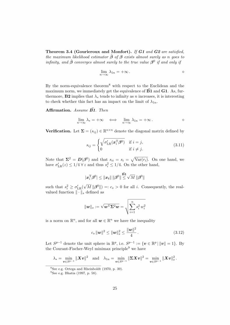
Theorem 3.4 (Gourieroux and Monfort). If G1 and G2 are satisfied,the maximum likelihood estimator β of β exists almost surely as n goes toinfinity, and β converges almost surely to the true value β0 if and only if

limn→∞

λ1n = +∞ . �

By the norm-equivalence theorem8 with respect to the Euclidean and themaximum norm, we immediately get the equivalence of �B1 and G1. As, fur-thermore, B2 implies that λ∗ tends to infinity as n increases, it is interestingto check whether this fact has an impact on the limit of λ1n.

Affirmation. Assume �B1. Then

limn→∞

λ∗ = +∞ ⇐⇒ limn→∞

λ1n = +∞ . �

Verification. Let Σ = (sij) ∈ Rn×n denote the diagonal matrix defined by

sij =

{√

σ′LR(xTi β0) if i = j,

0 if i 6= j.(3.11)

Note that Σ2 = D(β0) and that sii = si =√

Var(ri). On one hand, wehave σ′LR(z) ≤ 1/4 ∀ z and thus s2i ≤ 1/4. On the other hand,

|xTi β0| ≤ ‖xi‖ ‖β0‖

­B1

≤√M ‖β0‖

such that s2i ≥ σ′LR(√M ‖β0‖) =: cs > 0 for all i. Consequently, the real-

valued function ‖ · ‖s defined as

‖w‖s :=√

wTΣ2w =

√√√√

n∑

i=1

s2i w2i

is a norm on Rn, and for all w ∈ R

n we have the inequality

cs ‖w‖2 ≤ ‖w‖2s ≤ ‖w‖2

4. (3.12)

Let Sp−1 denote the unit sphere in Rp, i.e. Sp−1 := {v ∈ R

p | ‖v‖ = 1}. Bythe Courant-Fischer-Weyl minimax principle9 we have

λ∗ = minv∈Sp−1

‖Xv‖2 and λ1n = minv∈Sp−1

‖ΣXv‖2 = minv∈Sp−1

‖Xv‖2s .

8See e.g. Ortega and Rheinboldt (1970, p. 39).9See e.g. Bhatia (1997, p. 58).

25

Choose v∗ ∈ Sp−1 such that λ∗ = ‖Xv∗‖2. By (3.12) we have λ∗ =‖Xv∗‖2 ≥ 4 ‖Xv∗‖2

s ≥ 4λ1n. Conversely, if we choose v∗∗ ∈ Sp−1 suchthat λ1n = ‖Xv∗∗‖2

s, we get λ1n = ‖Xv∗∗‖2s ≥ cs ‖Xv∗‖2 ≥ cs λ∗. In

consequence, the inequality

cs λ∗ ≤ λ1n ≤ 14 λ∗ (3.13)

holds for all n, from where we get the affirmed equivalence. ¨

This result shows that B2 implies that λ1n also goes to infinity as n increases.The opposite, however, is not always true: Assume for instance that λ1n =cl lnn where cl > 0 is an arbitrary positive constant. By (3.13), we get thus

4 cl lnn ≤ λ∗ ≤clcs

lnn .

So while limn→∞ λ∗ = ∞, there is no positive constant c such that λ∗ > cnfor all n.

The assumption limn→∞ λ1n = ∞ of the theorem 3.4 is therefore less re-strictive than B2. Conversely, Gourieroux and Monfort (1981) need thesupplementary hypothesis G2 to prove the consistency of β. On the otherhand, G2 additionally ensures that limn→∞ λ1n = ∞ is not only sufficientbut also necessary for the consistency of β.

26

4 Asymptotic Normality of the Maximum Likeli-

hood Estimator

In the previous section, we have studied the consistency of the maximumlikelihood estimator in the logistic regression model. We were able to provethat, under certain hypotheses, the estimator β of β ∈ R

p converges inprobability to the true value β0.

A second important issue to be studied is the asymptotic normality of theestimator β. More precisely, we are going to show that the normalised linearcombinations of the components of β−β0 converge in distribution to randomvariables having a normal law with zero expectation.

The base structure of the following theorem is taken from an article byAntille and Rech (1999). Some extensions had to be made in respect of theheteroscedasticity of the components of r. On the other hand, the specificknowledge of σLR gave rise to several simplifications. In contrast to section 3,we now assume that the number p of exogenous variables is constant andthus independent of the sample size n.

Assumptions.

A1: The exogenous variables X are uniformly bounded, i.e. there exists apositive constant M such that |xij | ≤ M for all i ∈ {1, . . . , n} and allj ∈ {1, . . . , p}.

A2: If λ∗ denotes the smallest eigenvalue of the symmetric matrix XTX ∈R

p×p, there exists a positive constant c > 0 such that λ∗ > cn for alln. �

Theorem 4.1. Assume A1 and A2 and let D(β0) and Σ be defined as in(2.8) and (3.11) respectively. Then

eTXTD(β0)X(β − β0)

‖ΣXe‖L−−−→

n→∞N(0, 1)

for all e ∈ Rp with ‖e‖ = 1. �

Proof. From theorem 3.1 we know that, with a probability approaching 1as n→ ∞, the maximum likelihood estimator β is the unique solution of

−∇ lnL(β) = XT(σLR(Xβ) − y

)= 0 .

To simplify the notation we will thus assume that, for all n,

XT(σLR(Xβ) − y

)= 0 . (4.1)

27

This condition can be reformulated as

XT(

σLR

(X(β0 + β − β0)

)− y

)

= 0

⇐⇒n∑

i=1

xij

(

σLR

(xT

i β0

︸ ︷︷ ︸

=:γ0

i

+ xTi (β − β0)︸ ︷︷ ︸

=:εi

)− yi

)

= 0 ∀ j

⇐⇒n∑

i=1

xij

(σLR(γ0

i + εi) − yi

)= 0 ∀ j .

In application of the mean value theorem, we can write σLR(γ0i + εi) =

σ′LR(γ0i ) + εi σLR(ξi) where ξi = γ0

i + αi εi with αi ∈ ]0, 1[. This gives us theequivalent condition

⇐⇒n∑

i=1

xij

(εi σ

′LR(ξi) + σLR(γ0

i ) − yi︸ ︷︷ ︸

=−ri

)= 0 ∀ j .

Let e ∈ Rp with ‖e‖ = 1. We thus have

0 =

p∑

j=1

ej∑n

i=1 xij

(εi σ

′LR(ξi) − ri

)

‖ΣXe‖

= −p∑

j=1

ej∑n

i=1 xij ri‖ΣXe‖

︸ ︷︷ ︸

=:N1

+

p∑

j=1

ej∑n

i=1 xij εi

(σ′LR(ξi) − σ′LR(γ0

i ))

‖ΣXe‖︸ ︷︷ ︸

=:N2

+

p∑

j=1

ej∑n

i=1 xij εi σ′LR(γ0

i )

‖ΣXe‖︸ ︷︷ ︸

=:N3

.

(4.2)

Let us first show that N2P−−−→

n→∞0: We have

maxi∈{1,...,n}

|ξi − γ0i | = max

i∈{1,...,n}|γ0

i + αi εi − γ0i | = max

i∈{1,...,n}|αi x

Ti (β − β0)|

≤ xTi∗(β − β0) for an i∗ ∈ {1, . . . , n}.

By the inequality of Cauchy-Schwarz (C-S),

xTi∗(β − β0) ≤ ‖xi∗‖

∥∥∥β − β0

∥∥∥ =

√√√√

p∑

j=1

x2i∗j

∥∥∥β − β0

∥∥∥

A1

≤ √pM

∥∥∥β − β0

∥∥∥ .

28

Moreover, as β is consistent, ‖β − β0‖ P−−−→n→∞

0 from where it follows that

maxi∈{1,...,n}

|ξi − γ0i |

P−−−→n→∞

0 . (4.3)

Therefore,

|N2| =

p∑

j=1

ej∑n

i=1 xij εi

(σ′LR(ξi) − σ′LR(γ0

i ))

‖ΣXe‖

C-S≤ ‖e‖

‖ΣXe‖

√√√√

p∑

j=1

∣∣∣∣∣

n∑

i=1

xij εi

(σ′LR(ξi) − σ′LR(γ0

i ))

∣∣∣∣∣

2

≤ 1

‖ΣXe‖

√

p n2M2 ε2 maxi∈{1,...,n}

(σ′LR(ξi) − σ′LR(γ0

i ))2

=1

‖ΣXe‖√p nM ε max

i∈{1,...,n}

∣∣σ′LR(ξi) − σ′LR(γ0

i )∣∣

where ε := maxi∈{1,...,n} |εi|. For the denominator term, we get

‖ΣXe‖ =

√√√√

n∑

i=1

σ′LR(xTi β0)(Xe)2i ≥ ‖Xe‖ min

i∈{1,...,n}si

with si =√

σ′LR(xTi β0). However, on one hand,

|xTi β0| ≤ ‖xi‖ ‖β0‖

A1

≤ √pM ‖β0‖

such that s2i ≥ σ′LR(√pM ‖β0‖) =: c0. As, on the other hand, ‖Xe‖ ≥ √

cn(combine (3.8) with A2), it follows that

‖ΣXe‖ ≥ √c0 c n (4.4)

and thus

|N2| ≤1√c0c

√pM

√n ε max

i∈{1,...,n}

∣∣σ′LR(ξi) − σ′LR(γ0

i )∣∣ (4.5)

By the continuity of σ′LR we get with (4.3) that

maxi∈{1,...,n}

∣∣σ′LR(ξi) − σ′LR(γ0

i )∣∣ P−−−→

n→∞0 , (4.6)

and, by Cauchy-Schwarz again,

ε = maxi∈{1,...,n}

|εi| = maxi∈{1,...,n}

|xTi (β − β0)| ≤ √

pM ‖β − β0‖

29

Since p is fixed and thus XB(β0, δ) is bounded, there is a positive constantC > 0 such that

|aδpn(X,β0)| = | inf

“∈XB(˛0,δ)min

i∈{1,...,n}σ′LR(ζi)| ≥ C .

Therefore, as a conclusion of the remark on page 22,√n ‖β−β0‖ is bounded

in probability. The same holds thus for√n ε and we get with (4.5) and (4.6)

that

N2P−−−→

n→∞0 .

This result yields by (4.2) the condition

N1 +N3P−−−→

n→∞0 . (4.7)

Furthermore, we have

N3 =

p∑

j=1

ej∑n

i=1 xij εi σ′LR(γ0

i )

‖ΣXe‖ =

p∑

j=1

ej∑n

i=1 xij xTi (β − β0)σ′LR(xT

i β0)

‖ΣXe‖

=eTXTD(β0)X(β − β0)

‖ΣXe‖ .

As a result, if we can show that

−N1 =

p∑

j=1

ej∑n

i=1 xij ri‖ΣXe‖ =

eTXTr

‖ΣXe‖L−−−→

n→∞N(0, 1) , (4.8)

we have by (4.7) that N3L−−−→

n→∞N(0, 1). For this purpose, we write −N1 as

−N1 =

∑ni=1 ρi

‖ΣXe‖

where ρi := (Xe)i ri. We note that

n∑

i=1

Var(ρi) =

n∑

i=1

(Xe)2i Var(ri) =

n∑

i=1

(Xe)2i s2i =

n∑

i=1

(ΣXe)2i = ‖ΣXe‖2 .

Therefore, as a result of Lindeberg’s variant of the central limit theorem (seeFeller 1971, p. 262), (4.8) holds if the variances Var(ρi) satisfy the Lindebergcondition, i.e. for all t > 0,

n∑

i=1

E(ρ2i

∣∣ |ρi| ≥ t ‖ΣXe‖)‖ΣXe‖2

−−−→n→∞

0 . (4.9)

30

However, we have

Var(ρi)

‖ΣXe‖2=s2i (xT

i e)2

‖ΣXe‖2≤ s2i ‖xi‖2 ‖e‖2

‖ΣXe‖2≤ pM2

4 c0 c n−−−→n→∞

0 , (4.10)

the last inequality being a consequence of A1, (4.4), and the fact thats2i = σ′LR(xT

i β0) ≤ 14 . Finally, (4.10) implies (4.9), which completes the

proof. ¨

31

5 Case Study: Health Enhancing Physical Activ-

ity in the Swiss Population

In this last section, we shall study an example of applied logistic regression.In 1999, the Swiss Federal Offices of Sports and Statistics carried out anationwide survey of attitudes, knowledge and behaviour related to healthenhancing physical activity (HEPA)10. Based on recommendations11 of theSwiss Federal Offices of Sports and Public Health as well as the NetworkHEPA Switzerland they questioned 1,529 randomly chosen Swiss inhabitantsof at least 15 years of age. The samples for each of the German, French andItalian speaking parts of Switzerland were designed to have an equal size inorder to obtain results of comparable precision.

Two criteria were used to determine whether a person was physically ac-tive or not. First, people were asked whether they usually practised half anhour of moderately intense physical activity each day, which is consideredto be the base criterion for HEPA. An activity of moderate intensity is char-acterised by getting somewhat out of breath without necessarily sweating.Brisk walking, hiking, dancing, gardening and sports were stated as exam-ples for such an activity. In weighting the results accordingly to the languageregion, the age, the gender and the household size of the questioned persons,it was estimated that 50.6% of the Swiss population met the HEPA baserecommendations.

As a second criterion, people were questioned whether they practised regu-larly at least three times a week during twenty minutes or more a sportingactivity of vigorous intensity. This was the case for 37.1% of the Swisspopulation.

A person who met at least one of these criteria was designated as “physicallyactive”, a person who did not meet both of them was considered “physicallyinactive”. This information can now be represented for each person by thebinary variable yi. Let H = {hi}i∈{1,...,n} denote the set of the questionedindividuals. We define

yi :=

{

1 if hi is “physically inactive”,

0 if hi is “physically active”.

It has to be noted that, among the 1,529 questioned Swiss inhabitants,65 reported not to be able to walk a distance of more than 200 meterswithout outside help. These and five others who did not give answers to thecriteria mentioned above will not be taken into consideration. Therefore, nis assigned the value of 1,459.

10First results have been published by Martin, Mader and Calmonte (1999).11See Network HEPA Switzerland (1999).

32

In order to illustrate the application of the logistic regression model, weshall now analyse the impact of the linguistic regions of Switzerland onthe physical activity of their inhabitants. We divide H in three mutuallyexclusive sets HG, HF and HI containing the questioned inhabitants of theGerman, French and Italian speaking parts of Switzerland respectively. Forevery individual hi we define two indicator variables xFi and xIi by

xFi := 1HF(hi) and xIi := 1HI

(hi) ,

where 1S is the indicator function respective to the set S. Let us nowestimate the coefficients β0, β1, and β2 of the logistic regression model

logitπ = β0 + β1 xF + β2 xI .

For this purpose, we are going to minimise by the use of Mathematica theerror function Ey,σLR

defined as in (3.1) with respect to the given data set.Note that this procedure is absolutely equivalent to maximising the log-likelihood function, as has been shown in section 3.1. While the vector y

contains the variables yi defined above, the matrix X is constructed by therow vectors xT

i := (1 xFi xIi). The explicit values of y and X are notgoing to be displayed at this place. We assume that they are stored in theMathematica variables y and X. The vector β = (β0, β1, β2)

T is representedby the variable b:

b = {b0,b1,b2};

First of all, we assign the values of n and p:

{n,p} = Dimensions[X]

{1459,3}

In addition, the vector 1n, the primitive function HσLR, and the error func-

tion Ey,σLRare defined and stored in ev, H, and Err respectively:

ev = Table[1,{e,1,n}];H[z ] := Log[Exp[z] + 1]Err[b ] := ev.H[X.b] − y.(X.b)

Having specified y and X, it is now possible to print out the precise formof Ey,σLR

(β):

Err[b]

−721 b0 − 299 b1 − 261 b2 + 509 Log[1 + eb0

]+

485 Log[1 + eb0+b1

]+ 465 Log

[1 + eb0+b2

]

33

Finally, starting from β = 0, the function FindMinimum searches for alocal minimum in Ey,σLR

:

betahat = FindMinimum[Err[{b0,b1,b2}],{b0,0},{b1,0},{b2,0} ,WorkingPrecision− > 20]

{959.3452655931,{b0 → −0.770799,b1 → 1.2455,b2 → 1.0172}}

The estimated coefficients are thus βT = (−0.770799, 1.2455, 1.0172), andwe get the model equation

logitπ = −0.770799 + 1.2455xF + 1.0172xI .

For the interpretation of these coefficients, we take into consideration thecomments given in section 2.3.2. From there we know that the odds on theevent that y equals 1 increase (or decrease) by the factor expβi if xi growsby one unit. For people living in the German speaking part of Switzerland,both xF and xI are zero. Consequently, HG can be viewed as a “controlgroup” in the present investigation. Living in the French or Italian speakingpart of our country means from this viewpoint an increase of xF or xG byone unit respectively. We shall thus calculate the exponentials of β1 and β2:

{Exp[b1],Exp[b2]} /. betahat[[2]]{3.47466,2.76544}

As a result, the odds on an inhabitant of the French part of Switzerlandbeing physically inactive are almost 3.5 times as high as those of someoneliving in the German part. For the Italian in comparison to the Germanparts, the respective odds ratio is about 2.75.

As Martin and Mader (2001), both members of the Swiss Federal Office ofSports, state, these huge differences between the distinct linguistic regionsof Switzerland are astonishing. They assume that the perception of moder-ately intensive physical activity is influenced by each indiviual’s social andcultural background. The desirability of physical fitness is considered tobe particularly developed in the German part of Switzerland which couldhave lead to a considerable overreporting (overclaiming) among this groupof questioned people.

34

6 Conclusion

The example provided in section 5 gives a very rudimentary impressionof the power of applied logistic regression. The analysis of this specificapproach for modelling binary data within the scope of this thesis, however,has illustrated its versatility.

In the case of a fixed number of explanatory variables, both the consistencyand asymptotic normality of the maximum likelihood estimator are estab-lished under two comparably weak hypotheses. Both of them are technicalconditions with respect to the “layout” of the independent input variables.

If, on the other hand, the number of exogenous variables is allowed to growalong with the dimension of the sample space, it has been shown that therehad to be essentially a logarithmic relation between the former and the latterin order to maintain the consistency of the maximum likelihood estimator.

Even without an explicit quantification of this relation, this result providesan interesting insight into the interdependence of these two characteristics.

35

Acknowledgements

I would like to thank Prof Dr Andre Antille for the proposal of this interest-ing and many-sided topic as well as for his academic assistance during thedevelopment process of this diploma thesis.

Secondly, I want to express my gratitude to Prof Dr Bernard Marti, head ofthe Institute of Sports Sciences within the Swiss Federal Office of Sports inMagglingen, and to his collaborator Dr Brian W. Martin for placing at mydisposal the complete data set of the HEPA study used and referred to insection 5. Thanks also to PD Dr Hans Howald for arranging the necessarycontacts.

Finally, my appreciation goes to Manrico Glauser and Ralf Lutz for proof-reading this text and giving me precious feedback.

36

References

Amemiya, T. (1985). Advanced Econometrics, Harvard University Press,Cambridge.

Antille, A. and Rech, M. (1999). Learning Single Layer Neural Networks:Asymptotic Normality of Flat Spot Elimination Techniques, preprint.

Bhatia, R. (1997). Matrix Analysis, Graduate Texts in Mathematics,Springer, New York.

Christensen, R. (1997). Log-Linear Models and Logistic Regression, SpringerTexts in Statistics, 2nd edn, Springer, New York.

Collett, D. (1991). Modelling Binary Data, Chapman & Hall, London.

Cramer, J. S. (1991). The LOGIT model: an introduction for economists,Edward Arnold, London.

Feller, W. (1968). An Introduction to Probability Theory and Its Applica-tions, Vol. I, 3rd edn, John Wiley & Sons, New York.

Feller, W. (1971). An Introduction to Probability Theory and Its Applica-tions, Vol. II, 2nd edn, John Wiley & Sons, New York.

Garson, G. D. (2001). Statnotes: An Online Textbook [online], availablefrom: http://www2.chass.ncsu.edu/garson/pa765/statnote.htm.[Accessed 23 September 2001].

Gourieroux, C. and Monfort, A. (1981). Asymptotic Properties of the Max-imum Likelihood Estimator in Dichotomous Logit Models, Journal ofEconometrics 17: 83–97.

Hosmer, D. W. and Lemeshow, S. (1989). Applied Logistic Regression, JohnWiley & Sons, New York.

Kleinbaum, D. G. (1994). Logistic Regression: A Self-Learning Text, Statis-tics in the Health Sciences, Springer-Verlag, New York.

Martin, B. W. and Mader, U. (2001). Korperliches Aktivitatsverhalten inder Schweiz, preprint.

Martin, B. W., Mader, U. and Calmonte, R. (1999). Einstellung, Wissen undVerhalten der Schweizer Bevolkerung bezuglich korperlicher Aktivitat:Resultate aus dem Bewegungssurvey 1999, Schweizerische Zeitschriftfur �Sportmedizin und Sporttraumatologie� 47: 165–169.

Mazza, C. and Antille, A. (1998). Learning Single Layer Neural Networks:Consistency of Flat Spots Elimination Techniques, preprint.

37

McFadden, D. (1974). Conditional logit analysis of qualitative choice be-haviour, in P. Zarembka (ed.), Frontiers in Econometrics, AcademicPress, New York, pp. 105–142.

National Safety Council (2001). What Are the Odds of Dying? [online],available from: http://www.nsc.org/lrs/statinfo/odds.htm. [Ac-cessed 15 October 2001].

Network HEPA Switzerland (1999). Health Enhancing Physical Activ-ity HEPA (Recommendations) [online], Available from: http://

www.hepa.ch/english/pdf-hepa/Empf_e.pdf. [Accessed 10 Novem-ber 2001].

Ortega, J. M. and Rheinboldt, W. C. (1970). Iterative Solutions of NonlinearEquations in Several Variables, Academic Press, New York.

Santner, T. J. and Duffy, D. E. (1989). The Statistical Analysis of DiscreteData, Springer Texts in Statistics, Springer, New York.

38