Asymmetric effects of favorable and unfavorable information on decision-making under ambiguity

Alexander Peysakhovich  † and Uma R. Karmarkar  †

Most daily decisions involve uncertainty about outcome probabilities arising from

incomplete knowledge, i.e. ambiguity. We explore how the addition of partial information affects

these types of choices using theoretical and empirical methods. Our experiments in both gain and

loss domains demonstrate that when such information supports a favorable outcome, it strongly

increases valuation of an ambiguous financial prospect. However, when information supports an

unfavorable outcome, it has significantly less impact. We find that two mechanisms drive this

asymmetry. First, unfavorable information decreases estimates of a good outcome occurring, but

also reduces aversive uncertainty. These factors act in opposition, minimizing the effects of

unfavorable information. Second, when information can be subjectively interpreted, unfavorable

information is less likely to be integrated into evaluations. Our findings reveal mechanisms not

captured by traditional models of decision-making under uncertainty and highlight the importance

of increasing the salience of unfavorable information in uncertain contexts to promote unbiased

decision-making.

 

† These authors contributed equally to this work

2

Introduction

When a trader contemplates the value of a stock, or a manager chooses a potential

direction for company policy, their decision process rests on evaluating uncertain outcomes.

Uncertainty has been characterized using two dimensions: risk, the probability of a given

outcome, and ambiguity, the (un)availability of necessary information to estimate these

probabilities. Beyond distaste for risk, individuals also tend to be ambiguity averse in a way that

has seemingly irrational effects on decision-making (e.g. Ellsberg 1961, Camerer & Weber 1992,

Trautmann & van de Kuilen 2013). Much is known about how individuals respond to varying

levels of information in risky choices (e.g. shifts in probabilities; Camerer 1995, Kahneman &

Tversky 2000). However, it remains unclear how varying levels of available (but incomplete)

information affect decisions under ambiguity. In particular, in many situations it is possible for

an individual to receive partial information that is favorable or unfavorable to their desired

outcome, or even open to subjective interpretation. Such information may change the estimated

probability of a preferred outcome, but may also affect the perceived degree of aversive

ambiguity, making its impact difficult to predict. Here we employ experiments using financial

gambles to study how decision-makers integrate different categories and levels of incomplete

information to estimate value in ambiguous decisions.

To guide this work, we first adapt a simple model of ambiguity aversion to situations in

which levels of ambiguity can vary continuously. The model predicts that favorable information

(which supports a desired outcome) should have a larger impact on evaluations than unfavorable

information (which supports an undesired outcome). We test these predictions using paradigms

adapted from the “ball and urn” setup introduced by Ellsberg (1961), and commonly used in other

experimental work (e.g. Fox & Tversky 1995, Halevy 2007, Levy et al. 2010, Tymula et al. 2012

etc. ). In our experiments, outcomes of gambles depend on the color of a poker chip drawn from a

bag. The contents of each bag are fixed, but participants receive only partial information about

the composition. We vary the levels of this information parametrically from none (full ambiguity)

to complete (no ambiguity). We also consider a second, more subjective, paradigm in which

individuals evaluate ambiguous gambles based on the truth of a given trivia statement. Again, we

vary the information that individuals receive about the potential veracity of the trivia.

We find support for the model’s predictions such that favorable information has a larger

effect on behavior than unfavorable information in the domain of gains (experiments 1, 2) and the

domain of losses (experiment 3). We further demonstrate that this asymmetry persists when the

decisions are incentive compatible, and when they are centered on the evaluation of subjective

declarative statements (as opposed to numerical information; experiment 4). In experiment 5, we

3

provide insight into the psychological mechanisms driving this behavior. Our findings show that

evaluations of an ambiguous gamble are driven not only by the estimated likelihood of a positive

outcome occurring (as in a standard expected utility, or EU, model) but also by the certainty with

which the decision-maker feels they can estimate this probability. We show that unfavorable

information decreases estimates of a desired outcome occurring, but that it also reduces aversive

uncertainty. These two effects have opposing effects on the decision-maker’s valuations and

result in minimizing the overall impact of unfavorable information.

In a final set of analyses we examine mechanisms implied by a range of theories of

information processing under uncertainty. Our model includes an assumption of Bayesian

updating: that all information is incorporated in a rational manner. However, there is significant

evidence for both optimistic and pessimistic biases when information can be subjectively

interpreted (e.g. Lord et al. 1979, Peeters & Czapinski 1990, Jain and Maheswaran 2000,

Baumeister et al. 2001, Russo et al. 2004, Rozin & Royzman 2006). In our analyses, we indeed

find evidence for optimism bias when information needs to be subjectively interpreted, but not in

experiments where the partial information is numerical. Taken together, our findings represent

new insight into “nonstandard” responses to information in ambiguous decisions.

Ambiguity Aversion and Partial Information

Theoretical models of human decision-making under uncertainty often rely on subjective

expected utility theory (Savage 1971) combined with Bayesian updating. Specifically, individuals

begin with prior beliefs over possible states of the world and use incoming information to update

these priors in accordance with Bayesian inference (Kreps 1998). To make decisions, individuals

use these (updated) beliefs to form an expectation of possible outcomes and make a choice that

yields the highest expected utility.

A key challenge to this model of decision-making comes from the Ellsberg paradox

(Ellsberg 1961). As a generalized description, suppose participants are presented with a container

of 100 poker chips, all of which are either red or blue. They are asked for their willingness to pay

(WTP) to play a game in which they guess the color of a chip drawn from the bag at random.

Players win a monetary reward if the color of the drawn chip matches their guess, but receive

nothing if it does not. On average, individuals are willing to pay more in situations when there is

no ambiguity. For example, if a person has the knowledge that a bag contains exactly 50 red and

50 blue poker chips (no ambiguity) they value it more highly than a bag where they have no

information about its contents (complete ambiguity). This occurs even though individuals

4

maintain the same risk estimate for a chip of their color being drawn, contrary to the predictions

of SEU theory.

We now model an environment in which levels of ambiguity arising from the amounts of

both favorable and unfavorable information can vary continuously. This allows us to formalize

how differing amounts of partial information may affect ambiguous decisions. To do so, we have

chosen a particular model of ambiguity aversion used in previous experimental work: a version of

the maximin model of Gilboa & Schmeidler (1989).1

Consider a decision-maker (DM) facing an ambiguous financial prospect (AFP): an AFP

includes a single prize z, a set of states of the world represented here by the interval [0,1] and a

winning function γ:[0,1] to [0,1]. Given a state of the world w, the probability of winning the

prize z (i.e. the risk of the ambiguous prospect) is given by γ(w). The states are ordered such that

γ is increasing, namely higher states always mean a (weakly) higher probability of winning the

prize.

The DM, or agent, does not know w but receives partial knowledge about what it could

be. We restrict this to a particular kind of partial knowledge. Specifically, the DM can

conclusively rule out that the state is less than some threshold X, thus we define X as the amount

of favorable information. In addition, the DM can rule out that the state is greater than Y, thus we

define Y as the amount of unfavorable information. The vector (X, Y, γ, z) completely

parameterizes the AFP. We are interested in responses to information, so in the following

discussion we fix the winning function and z. We suppress the dependence on γ and z in all later

notation.

The agent has no explicit information about the likelihood of states that are deemed

possible. For intuition, the pair (X=0,Y=0) represents that the agent knows nothing about the

possible state of the world, while (X=.5, Y=.5) means that the state of the world must be

exactly .5. In comparison, (X=.25, Y=.25) means that the state must be somewhere in the interval

[.25, .75] but the DM has no other information about what it could be. Restricting to this type of

knowledge allows us to explicitly vary levels of ambiguity in our experimental designs.

                                                                                                               1  We choose this model because it is straightforward to work with and has been used in other experiments involving paradigms similar to ours (e.g. Levy et al. 2010, Tymula et al. 2012). We acknowledge that there are several other potential choices, including rank-dependent utility (Segal 1987), second-order expected utility (Grant et al. 2009), expected uncertain utility theory (Gul & Pesendorfer 2014), variational preferences (Maccheroni et al. 2006), smooth ambiguity models (Klibanoff et al. 2005) and others. At their core, each of these models captures ambiguity aversion by postulating that second-order uncertainty is somehow aversive. We conjecture that these models would generate similar behavioral predictions. Testing this conjecture, and the possibility that our results and experimental paradigm could also help to discriminate among these models provides an important avenue for future work.  

5

The DM evaluates an AFP as follows. The prize is worth utility u(z), which we set to be 1

without loss of generality. The DM has a subjective probability distribution p(X,Y) on the set of

all states. To build this distribution p(X,Y) we assume the DM begins with a full-support prior p0

on the state space and updates it in accordance with Bayes rule given the knowledge (X,Y) he has.

We now apply a version of the maximin utility function introduced in Gilboa &

Schmeidler (1989). First, we simplify notation and let P(X,Y) be the DM’s subjective probability

of winning the prize z given (X,Y). This can be derived from the primitives as follows:

P(X,Y) = ∫γ(w)dp(X,Y) [eq. 1]

We assume that p is well-behaved and so is continuously differentiable in X and Y. The

DM’s utility for an AFP (X,Y) is

W(X,Y) = (1-λ(X+Y))P(X,Y) [eq. 2]

where λ(X+Y) is a smooth, decreasing function from [0,1] to [0,1] that has λ(1) = 0. This

means that if λ is identically zero, the DM acts as an EU agent. Note also in the case of uncertain

decisions with no ambiguity (that is, when X + Y = 1) the DM also behaves as an EU maximizer.

However, when X+Y is less than 1 the DM “downweights” the probability P(X,Y) and so behaves

in an ambiguity averse manner.

We can now look at the effects of changes in X and Y on evaluation in the AFP.2 In

particular, we are interested how ambiguity averse (AA) agents differ from EU agents. Without

making functional form assumptions on λ we cannot draw the exact form of their indifference

curves; however, we can still show local properties of the agent’s evaluations. We now consider

the comparative statics of the valuation of a prize with respect to X and Y. Fixing a knowledge

level (X,Y) and differentiating gives us the marginal effects of favorable and unfavorable

information:

∂W(X,Y)/∂X =(1-λ(X+Y))∂P(X,Y)/∂X - ∂λ(X+Y)/∂X*P(X,Y)[eq. 3]

∂W(X,Y)/∂Y =(1-λ(X+Y))∂P(X,Y)/∂Y - ∂λ(X+Y)/∂Y*P(X,Y) [eq. 4]

                                                                                                               2  We note here thatλrepresents a fixed preference (or aversion) to ambiguity and what we assume varies is the amount of ambiguity, not the individual’s attitude toward it.  

6

The comparative statics clearly show that two effects operate on AA DMs. We call these 1) the

likelihood effect (captured mostly by the first term) and 2) the certainty effect (captured in the

second term).

The intuition behind this is as follows: favorable and unfavorable information change the

estimates of winning P(X,Y) in the obvious directions but also reduce ambiguity (decrease λ

(X+Y)). Thus the net effect of changing X and Y depends on both of these elements. The

likelihood and certainty effects push in the same direction for changes in X but in opposite

directions for changes in Y.

This stylized model allows us to draw the following specific hypotheses that can be tested

behaviorally:

H1: In evaluating AFPs, changes in favorable information (X) will have

more impact on valuation than changes in unfavorable information (Y).

This hypothesis, though simply stated, has the potential to cover a broad range of

scenarios. For example, we posit that the asymmetry between favorable and unfavorable

information should persist in the domains of both gains and losses and across different

specifications of AFPs. Thus we devote experiments 1-4 to establishing support for this

hypothesis and its generalizability.

While H1 predicts the overall expected behavioral outcomes, the model also motivates

hypotheses about the potential underlying mechanisms. It first suggests that individual’s

valuation will depend on their assessed probability of a desirable outcome occurring (captured by

P(X,Y)) as well as the amount of residual ambiguity of the situation (captured by λ(X+Y)). We

refer to these two as subjective likelihood estimates and subjective certainty in what follows. This

leads to our second hypothesis:

H2: Subjective likelihood estimates and subjective certainty will have

positive effects on valuation of AFPs.

Further considering the shape of the functions allows us to make predictions about the

effects of favorable and unfavorable information on other psychological variables. The subjective

likelihood of winning the prize (i.e. P(X,Y)) is affected positively by X and negatively by Y. Felt

certainty (i.e. 1-λ(X+Y )) increases in both X and Y. Note that this increase in certainty about the

7

situation should reduce its aversiveness, and also contribute to increases in WTP. This yields the

following two hypotheses:

H3a: Favorable (unfavorable) information will increase (decrease)

subjective estimates of the likelihood of winning the prize.

H3b: Both favorable and unfavorable information will increase felt certainty.

Alternate accounts of biased information processing

Stepping back from the formalization, a key assumption of our model is that the agent’s

belief distribution incorporates information in a “neutral” manner (here modeled using Bayesian

updating of a prior). Since Bayesian updating considers all information as equal, the model

predicts no preferential bias towards the integration of one “type” of information. However,

literature across multiple disciplines has shown that this prediction fails in several environments.

Experiments on information integration in affectively charged domains such as political opinions

(Lord et al. 1979, Westen et al. 2006) or consumer brand preferences (Jain and Maheswaran 2000,

Russo et al. 2004) find a bias for confirming information, which supports existing attitudes, over

conflicting information which counters them. Other findings suggest that positive information or

feedback about one’s own desirable personal attributes is similarly overweighed (Sharot et al.

2012, Eil & Rao 2012).

In domains such as preference and attitude formation, a number of studies have also

shown that a Bayesian updating prediction fails in the opposite direction. In particular, negative

information about a product or individual is given disproportionate consideration, sometimes

even resulting in negative evaluations despite a clear majority of positive attributes (Peeters &

Czapinski 1990, Baumeister et al. 2001, Rozin & Royzman 2006). Overall, these literatures raise

the possibility that individuals may respond asymmetrically to information about gains and losses

in the domain of ambiguity. However, the conflicting predictions give little insight into what kind

of bias should be expected or how this might interact with individuals’ general aversion to

ambiguity. Thus in addition to the model-driven predictions, we examine an additional

exploratory hypothesis, motivated by the broader multidisciplinary study of information

processing and valence asymmetries.

H4: Individuals bias their information processing such that they directly

overweight the contribution of favorable or unfavorable information under

uncertainty.

8

We note that our predictions H1-H4 have the potential to conflict with one another, or to

hold true in some decision contexts, but not others. Thus we tested these hypotheses in a series of

behavioral experiments, summarized in Table 1. In each experiment, participants were presented

with multiple AFPs. We varied the levels of favorable and unfavorable information available and

investigated the effects of this variation on the participants’ subjective evaluations of the

prospects, as measured by willingness to pay (or willingness to purchase).

Experiment 1: Effects of partial information in the domain of gains

To address the central hypothesis emerging from our model (H1), we examined how

individuals valued hypothetical ambiguous gambles depending on partial information that

supported or argued against a winning (desired) outcome.

Methods

One hundred and seventeen individuals (61% male, Mage=32.93) were recruited for this

study via Amazon Mechanical Turk3 (AMT). Compensation was fixed across participants, based

on the estimated duration of the experiment, and independent of choices made or performance in

the task. Participants provided informed consent in accordance with the IRB standards of the

supporting university. They engaged in the central experimental task (see below) and then

reported basic demographic information.

At the beginning of the experiment, participants were asked basic comprehension

questions about the rules of the experimental task. Seventeen participants were unable to

successfully complete these questions, and were removed from the analysis, leaving a sample size

of n = 100.

Participants engaged in an experimental paradigm adapted from the paradox proposed by

Ellsberg (1961). In this “pull-a-chip” game, they were informed that they were making choices

about a bag of exactly 100 chips, each colored red or blue, and that one chip would be pulled

from the bag at random. Participants were asked to imagine that drawing a red chip would result

in winning $50, and that drawing a blue chip would result in winning nothing. The “pull-a-chip”

game can be written formally using our model by discretizing the state space to be {0, 1, …, 100}

                                                                                                               3 The use of AMT for experimental research is relatively new and reflects a unique subject pool (e.g. Paolacci & Chandler 2014, Rand et al. 2014). Recent work demonstrates the validity of the experimental data collected with AMT for economic games involving hypothetical and minimal ($1) stakes (Amir & Rand 2012). Furthermore, behavior on AMT matches well with standard laboratory results on economic risk/gambling tasks (e.g. Fudenberg & Peysakhovich 2014, Imas 2014).

9

with γ(w)= w/100. We implemented varying levels of knowledge by presenting participants with

statements of the form: “You know that the bag contains at least X red chips and at least Y blue

chips.” Thus X was the amount of favorable information, and Y was the amount of unfavorable

information. X and Y were varied parametrically from 0 to 50 in increments of 25, creating 9

possible levels of knowledge, or rounds.

All participants entered their hypothetical willingness to pay (WTP) for tickets to play in

each of the 9 rounds by moving a slider on a scale that ranged from $0 to $35 in $1 increments.

Each round was presented on its own page, and participants had to indicate their responses before

moving on to the next decision. For their first decisions, all participants evaluated rounds

specified by (0,0) and (50,50) to allow for a direct test of the Ellsberg paradox across individuals.

Results

We examined the (0,0) and (50,50) gambles to benchmark our findings. Consistent with

ambiguity aversion, average WTP was significantly lower for a ‘pull-a-chip’ bag with no chip

information given at all (M= 4.22, SD=5.32) 4 compared to a ‘pull-a-chip’ bag with a known

composition of 50 red chips and 50 blue chips (M=10.98, SD=8.78; t-test p<.001). We note that

even though this design is hypothetical, the reported WTP matches well with existing work on

ambiguity aversion in recent incentive compatible experiments (Tymula et al. 2012, see Appendix

Section 1 for calibration details).

We now turn to investigating the effects of partial information on reported WTP. Recall

that red is the winning color. Thus, the number of red chips represents the amount of favorable

information, and the number of blue chips represents the amount of unfavorable information

received. Visualizing the data in Figure 1 appears to show that adding favorable information

increases WTP more than adding equivalent amounts of unfavorable information decreases WTP.

We ask whether this result survives statistical analysis. As a first cut, we used a reduced form

model to estimate the average marginal effect of favorable vs. unfavorable information on WTP.

We regressed WTP on the amount of favorable and unfavorable information present (e.g. the

numbers of red and blue chips). The coefficients in these regressions can then be interpreted as

average marginal effects of information type on WTP. Note that the design is such that both the

number of red chips (X in our formalization) and the number of blue chips (Y) are drawn from

the set {0, 25, 50}. As neither one exceeds 50, choosing a value for X (or Y) does not constrain

                                                                                                               4 M is used here and going forward as an abbreviation for “Mean”.

10

the other variable. Since participants enter decisions for each possible knowledge level, X and Y

are uncorrelated variables in our regressions.

These analyses (Table 2, column 1) revealed that favorable information had a large

positive effect on WTP. On average, adding a marginal red chip increased WTP by 13.3 cents. In

contrast, unfavorable information had no (significant) effect (point estimate = .6 cents). The

absolute magnitude of unfavorable information’s effect was significantly smaller than the effect

of favorable information (test for equality of regression coefficients p<.01) revealing a large

asymmetry between the impact of different information types. Since less than 2% of the

decisions for any gamble include a WTP of 0, it is unlikely that our findings are due to censoring

at 0 in the responses.

In addition to the regression-based analysis, we appealed to the theoretical results derived

in the model section to motivate a reduced form “difference-in-difference” analysis. First, let us

fix an AFP and define WTP(X, Y) as the willingness to pay of an agent when she is faced with

information levels given by (X, Y). Note that the simple model of ambiguity aversion implies that

at any (X, Y) the marginal addition of favorable information should have a larger effect than the

marginal addition of unfavorable information. Note that because this property always holds on the

margin, it must also hold for any non-marginal quantity d. Thus, we should expect to see that an

increase in favorable information by d should have a larger positive impact on WTP than the

comparable negative impact from increasing unfavorable information by d. Formally this can be

written as:

WTP(X+d, Y) – WTP(X,Y) > -(WTP(X, Y+d) – WTP(X,Y))

We use this basic fact to motivate our next hypothesis test. We initialize at a point (X,Y)

and define two empirical quantities from our data:

ΔPos(X,Y) = mean[WTP(X+25, Y)] – mean[WTP(X,Y)]

and

ΔNeg(X,Y) = mean[WTP(X, Y+25)] – mean[WTP(X,Y)]

We then ask whether there is a stronger effect of increasing favorable information by 25 than by

increasing unfavorable information by 25. Formally, we are testing the following: on average,

over all possible starting positions, is mean[ΔPos(X,Y) + ΔNeg(X,Y)] > 0?

11

Performing the analysis showed that the empirical difference between ΔPos(X,Y) and

ΔNeg(X,Y) is approximately $3.76. This is significantly different from 0, with a participant-level

bootstrapped 95% confidence interval = [2.93, 4.56]. Thus, both types of analyses show that

favorable information has a greater impact on the valuation of financial prospects than equal

amounts of unfavorable information.

Experiment 2: Effects of Partial Information, Allowing for Choice of Winning Color

In contrast to many prior experiments on ambiguity aversion (see Trautmann & van de

Kuilen 2013 for a recent review), we pre-assign red as the winning color in experiment 1. We

thus performed a second experiment in which participants were able to view the available

information and select both their WTP and which color would correspond to a winning outcome.

Methods

One hundred and twenty-two individuals (59% male, Mage=31.89) were recruited for this

study via AMT with general procedures (compensation, consent, and demographics) occurring as

in experiment 1. Participants engaged in a “choice” version of the pull-a-chip task. The

instructions explained that participants could buy a ticket to play in a game where 1) they would

have selected the color for the winning chip and 2) a chip would be drawn at random from the

bag. Given this procedure for the game itself, for each round, participants viewed information

about the contents of the bag. They then indicated their WTP to play (by moving a slider on a $0-

$35 scale) and indicated the color they would choose if the round was played. At the beginning

and end of the experiment, participants were asked basic comprehension questions about the rules

of the experiment. Eleven participants were unable to successfully answer one of these questions

and were removed from the analysis, leaving a sample size of n = 111.

Results

Given that participants selected the winning color each game, for each participant

decision we designated information about the chosen (winning) chip color as “favorable” and

information about the non-chosen chip color as “unfavorable”. We regressed WTP on the number

of chips of the chosen winning color (#favorable) and number of chips of the non-winning color

(#unfavorable) as in experiment 1. As shown in Table 2 (col.2), unfavorable information had a

significantly smaller effect on WTP than favorable information (Test for equality of regression

coefficients p<.01). Thus we find support for H1 regardless of whether individuals themselves

select which color will indicate a winning outcome.

12

Experiment 3: Effects of partial information in the domain of losses

In experiments 1 and 2, a winning outcome resulted in a net financial gain (higher than

the endowment) and a losing outcome resulted in receiving no gain (or “losing” only the ticket

price.) However, in a context of uncertainty, reframing a gamble as a pure loss rather than a pure

gain can lead individuals to engage in risk-seeking behavior (e.g. Kahneman & Tversky 1979,

Kahneman & Tversky 2000). Somewhat relatedly, in the first two experiments, favorable

information is highlighted by the gain frame of the decision. Thus, though our findings are most

consistent with overweighting favorable information, they cannot rule out the possibility that

participants’ behavior is driven by overweighting the outcome-salient information (e.g. Wason

1966). Motivated by these issues, we conducted an additional experiment to examine whether

our effects carried over to the domain of losses.

Methods

Sixty individuals (MAge = 33.35, 58% male) were recruited via AMT, with general

procedures occurring as in experiment 1. At the beginning and end of the experiment,

participants completed attention checks consisting of copying text into a response box and

answering basic comprehension questions about the rules of the experiment. Seven participants

were unable to successfully complete at least one of these tasks, and were removed from the

analysis, leaving a sample size of n = 53.

Participants engaged in a loss-based version of the pull-a-chip task. They began each of

9 rounds with a hypothetical endowment of $50, and the assumption that at the end of a round a

chip would be drawn from a bag of 100 red or blue chips. They were informed that if the drawn

chip were red, they would lose their endowment, and if it were blue, they would keep their

endowment. Participants were asked to report their WTP for an insurance ticket (using a slider

from $0-35 in $1 increments), which would protect their $50 endowment if a red chip were drawn

and have no effect otherwise. The nine rounds/knowledge levels were implemented in a manner

identical to experiment 1. All participants completed all levels, creating a within-subject design.

Results

Note that the measure of WTP for insurance tickets in this experiment behaves in the

opposite direction from gamble tickets in the first experiment. Thus, a more negative evaluation

of the gamble (e.g. a higher chance of losing endowment) should increase WTP for insurance

while a more positive evaluation (e.g. lower chance of losing endowment) should decrease WTP

13

for insurance.

If our previously observed asymmetry is driven by a bias towards “confirming” or

outcome-salient information, then a loss frame should lead to overweighting information that

suggests that a loss is more likely. If the asymmetry is driven by a bias towards favorable

information, it should lead to overweighting information that suggests a loss is less likely.

Regressing WTP for insurance on the amount of no-loss (favorable) and loss (unfavorable)

information revealed that the number of no-loss chips had a significant negative influence on

WTP for insurance. In contrast, the number of loss chips had no significant effect (Table 2, col. 3).

These data suggest our main effect specifically involves overweighting information about an

individual’s favored outcome rather than the salient outcome.

To explore whether participants show behavior consistent with interpreting our design as

a loss frame, in Appendix Section 1 we calibrate individual level risk-aversion parameters as in

experiment 1. We see that indeed individuals indeed display convex utility functions (ie. risk-

seeking behavior). Thus our evidence shows that overweighting favorable information appears to

occur in the domain of loss, and suggests that it is not disrupted by loss aversion or the shift in the

gambles’ reference point.

Experiment 4: Subjective perceptions of information and incentive compatible gambles

The findings in experiments 1-3 reflect hypothetical situations. However, decisions with

real consequences can be more representative of daily decision-making, and can elicit stronger

reactions than hypothetical scenarios (Bushong et al. 2010, Kang et al. 2011). In this study, we

utilized a within-subject design with an incentive compatible valuation procedure and prizes that

resulted in real monetary outcomes.

To further widen the scope of our findings, we examined two additional types of

ambiguous decision-making beyond pull-a-chip games. First, we note that the “pull-a-chip”

game includes both risk and ambiguity; here, perfect knowledge of a bag’s contents does not

guarantee knowledge of whether the outcome would be a win or loss. As our model-derived

theory applies to arbitrary AFPs, we included a “majority game” in which the AFP is a bag of 101

poker chips (all red or blue). To determine the outcome, the bag is emptied and the color of the

majority of the chips (>50) determines whether the participant has won or lost. Here, because

knowledge of the bag’s contents completely describes whether the outcome is a win or loss, the

majority game includes ambiguity, but does not include risk.

Second, in the games based on considering specific quantities of poker chips, there is

little room for subjective interpretations of the information and there is a known cap on the

14

available amount of information. To better understand whether our findings carried over to less

“calculable” contexts, we tested how individuals processed more complex information related to

real world trivia (see Methods below).

General Methods

Thirty-seven university students (MAge=21.8, 38% male) completed this in-person study

at a computer laboratory with a known policy preventing the use of deception. They were seated

individually at computer terminals, separated by dividers. Participants provided informed consent

in accordance with the IRB standards of the supporting university. All participants received $10

in compensation for participating in the study. In addition, they were endowed with 25 points at

the start of the experiment, with the potential to spend those on game rounds where winning

outcomes yielded 30 points. Points were translated into dollars at the end of the experiment (at a

rate of 4 to 1), allowing participants to earn up to approximately $14 depending on their choices

and the gamble outcomes. The experiment consisted of two parts: (1) AFPs based on poker-chip

games and (2) ambiguous gambles based on trivia items (see 4A and 4B below). Each part was

subdivided into rounds.

Across the experiment, true WTP was elicited via a version of the Becker-DeGroot-

Marschak (BDM) procedure (Becker et al. 1964). Participants were given an endowment of 25

points at the start of each round, and asked to enter in any amount of this as their WTP. At the

start of the experiment, they were given detailed instructions explaining that their indicated WTP

would be compared with a price randomly generated by the computer. If the computer’s price was

higher than their stated WTP, they retained the full endowment for that round. If the computer’s

price was lower, they bought the ticket out of their endowment for that price. To prevent

“portfolio building” only one round of the experiment (from parts A and B combined) was chosen

to count for real money and was actually played at the end of the experiment for each participant.

Participants received no feedback on any of their choices until this time. Participants’ choices

were honored based on the outcome, and cash payouts were delivered accordingly.

To address any potential concerns about experimenter dishonesty, the winning color (red

or blue) for each poker-chip gamble was chosen randomly. Participants were informed of this

design, as well as the reasons behind it. A similar outcome-assignment randomization method

was used in the trivia-based gambles.

Experiment 4A.

Methods

15

Participants evaluated both pull-a-chip games and “majority games” in which they made

choices about bags of poker chips, with all chips colored red or blue. At the start of a round,

participants were informed of that round’s (randomly chosen) “winning color”. For pull-a-chip-

games, participants were informed they would win 30 points if a randomly drawn chip from the

bag matched the winning color. For majority games rounds, winning was determined by

emptying the bag at the completion of the experiment. Here, participants would win 30 points if

the majority of the chips out of the 101 in the bag matched the winning color, and receive nothing

otherwise. The majority game can be written formally in our framework by letting the state space

be {0, 1, …, 101} and the winning function is described by γ(w)= 0 if w<51 and γ(w)= 1

otherwise.

Knowledge levels were implemented as in experiment 1. Each participant made a total of

18 choices (9 levels of knowledge x 2 types of games). The rounds were presented in random

order with the following exception: the first evaluation for all participants was the pull-a-chip bag

whose contents were known to be 50 red chips and 50 blue chips and their second evaluation was

the pull-a-chip bag with no information. For each pull-a-chip and majority bag presented to them,

participants indicated how much they would be willing to pay for a ticket to play in that gamble

using a text entry box. Additionally, participants were asked for their confidence that they would

win each game.

Upon entering the experimental room, participants viewed 18 real bags that had each

been filled with poker chips accurately corresponding to the information given in for each round.

Participants had their attention specifically directed to these bags both in their written instructions

as well as verbally by the experimenter. Though participants were not able to view the contents of

the bags, a randomly chosen bag was shaken to demonstrate that it did contain poker chips. These

bags remained present in the room for the duration of the experiment to address any concerns

about the “real” nature of the gambles, or experimenter deception.

Results

Our data was again consistent with standard predictions of ambiguity aversion: WTP for

a pull-a-chip bag with no information (M=6.27, SEM = .88) was significantly lower than that for

a pull-a-chip bag with a known composition of 50 red and 50 blue chips (M=10.40, SEM =.86; t-

test p<.001). Levels of risk aversion and ambiguity aversion behavior were consistent with other

recent empirical papers (see Appendix Section 1 for calibration and discussion).

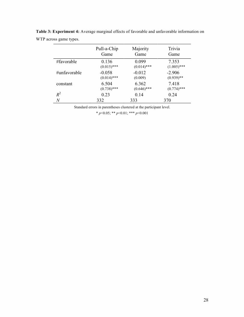
Regressing WTP on the amounts of favorable and unfavorable information showed that

the asymmetric effects of favorable and unfavorable information persisted for pull-a-chip games

16

under incentive compatible conditions (Table 3 col. 1; Test for equality of regression coefficients’

magnitudes p< .01). We observed this asymmetry in the majority game as well (Table 3 col. 2;

Test for equality of regression coefficients’ magnitudes p < .01). Thus our results replicate across

numerous samples, and hypothetical and incentive compatible contexts.5 As before, the effect

cannot be explained by censoring, as only 12% of WTP decisions are zero and the effect is robust

to using a Tobit regression. Furthermore, repeating the difference-in-difference analysis detailed

in experiment 1 similarly showed that increasing favorable information by 25 chips had a larger

impact than increasing unfavorable information by 25 (difference = 3.76, bootstrapped 95%

confidence interval: [2.92, 4.63]).

Experiment 4B

Hsu et al. (2005) show that both behavior and neural activity in trivia-based ambiguous

gambles are very similar to standard Ellsberg-based designs.  To examine how our observed

biases might manifest in such a context with more “subjectively” interpretable information,

participants from experiment 4A also engaged in the following decisions.  

Methods

Participants judged gambles dependent on trivia drawn from categories such as sports,

geography, finance, weather and knowledge of cities, along with up to two relevant facts (e.g. Fig.

2A, see Appendix Section 2 for all questions and facts used in the experiment). To rule out

participant concerns related to unfair experimental conditions or “rigging”, trivia items were

always in the form of whether a particular quantity (e.g. value of the DOW in a given year) was

above or below some threshold. To prevent the threshold from acting as a signal, the winning

“direction” (above or below) was randomly assigned at the question level (e.g. for all participants

roughly half of the trivia reflected “above” and half reflected “below”). Participants were

informed of this randomization both verbally and in their written instructions.

All individuals saw 10 pieces of trivia (see Appendix Section 2 for listing) in a random

order. For each trivia item, they were randomly assigned to see either 0,1 or 2 related facts.

Participants were informed that if the trivia statement was true, they would win additional money.

If it was false, they would win nothing. After indicating their WTP to play each trivia gamble

(using the same BDM procedure as 4A), participants rated their confidence that they would win                                                                                                                5 We note that the size of the asymmetry is different between our hypothetical and incentive compatible experiments. This could be due to the incentivized nature of our lab replication or due to changing subject pools (individuals on AMT vs. mostly Harvard undergraduates). Though these findings do not reveal the exact nature of the moderators, they illustrate that the asymmetry between favorable and unfavorable information appears to be quite robust.

17

on a scale of 1 [Not very confident] to 7 [Extremely confident] as well as how knowledgeable

they felt about the topic of the trivia question on a scale of 1 [Not very knowledgeable] to 7

[Extremely knowledgeable]. When participants received facts along with the trivia, they

categorized those facts as favorable (“This fact makes me think that it is more likely that the trivia

is true”), unfavorable (“This fact makes me think that is it less likely that the trivia is true”) or

neutral/unimportant (“This fact does not help me make any judgment on the trivia”).

Results

To analyze the effect of information in the trivia games, we used the subjective

categorization of the related facts as favorable or unfavorable at the individual level. We excluded

facts rated as neutral/unimportant being excluded (approximately 66% of presented facts were

rated as favorable or unfavorable). We pooled the analysis across the 10 trivia items. Figure 2B

shows that information categorized as favorable once again exerted a strong positive effect on

WTP while information categorized as unfavorable had a negative but weaker effect. Regression

analysis (Table 3) revealed that the effect of favorable information was significantly larger than

the effect of unfavorable information (absolute magnitude=38%, Test for equality of regression

coefficients p<.01). This analysis is robust to the addition of demographic controls (see Appendix

Section 1).

This design is a strong test of the asymmetric effects of favorable information on value.

Participants state that information they categorize as unfavorable makes them think that the trivia

item is less likely to be true. However they do not appear to adjust their WTP nearly as much as

in response to such unfavorable information as they do in response to favorable information. We

also found no significant impact of information on perceived knowledgeability of the topic,

suggesting that information is not simply increasing familiarity with the general trivia domain

(see Appendix Section 1).

As a robustness check, we also looked for relationships between poker-chip and trivia

behavior. To do this we calibrated a two parameter (risk aversion, ambiguity aversion) power-

utility based function at the individual level using part 1 data. We found that individual level risk

aversion correlated positively with WTP for trivia gambles while calibrated individual-level

ambiguity aversion correlated negatively, providing confirmation that the trivia based gambles

indeed seem to tap into individual preferences for risk and ambiguity. For full details of the

structural estimation and the accompanying analysis, see the Appendix (Section 1).

Overall, experiments 1-4 have provided strong support for H1. In particular, across a

variety of domains, favorable information has a much stronger effect on valuations of AFPs than

18

unfavorable information. Our trivia experiment demonstrates that this effect holds in situations in

which the information provided is “subjective,” or non-numerical, and thus less open to

calculations. Given this support for our proposed model, we turned to investigating hypotheses

H2-H4 and the psychological mechanisms underlying this behavioral effect.

Experiment 5: Information and aversive uncertainty

The nature of ambiguity aversion suggests a mechanism underlying our observed

asymmetry: namely a powerful aversion to ignorance (e.g. Fox & Tversky 1995, Frisch & Baron

1988). In our experiments, individuals are aware that they are using incomplete information to

estimate outcome probabilities. Thus they are aware that these estimates may not be accurate. Our

model suggests that increases in the subjective likelihood of a winning outcome and increased felt

certainty in estimates of outcome likelihoods should increase valuation of AFPs (H2), and thus

WTP.

Hypotheses 3A and B, motivated by our model, specify how information should affect

these two variables and how they would drive our main behavioral findings. They indicate that

favorable information has two potentially positive effects: increasing the subjective probability of

a good outcome and also increasing felt certainty. They also predict that unfavorable information

has two effects that potentially act in opposition. Unfavorable information can decrease the

subjective probability of a good outcome, but it can also increase felt certainty, releasing

individuals’ aversion to ignorance. Thus unfavorable information’s net impact on WTP is reduced.

Figure 3 summarizes this model in the form of a directed graph, which is tested in the following

study.

Methods

Twenty-nine university students from the local metropolitan area participated in this

experiment (Mage=21.85, 60% male)6 in a computer laboratory with a known policy preventing

the use of deception. Participants provided informed consent in accordance with the IRB

standards of the supporting university and received $15 in monetary compensation for

participation. Detailed instructions were provided for each element of the experimental task.

Individuals were presented with two blocks of 50 pull-a-chip rounds (for a total of 100 rounds) in

a within-subject design. This large number of rounds allows us to verify whether our effect is

robust to experience with the decision problem. Rounds were generated randomly as follows: we

                                                                                                               6  Four participants declined to give their gender and two participants declined to give their age in the post-experimental questionnaire. The reported compositions include only those who reported this information.  

19

started with a ‘center’ from the set (0,0), (50, 0), (0, 50) and (50,50). We then added uniformly

distributed noise with support in the interval [-20, 20] to both favorable and unfavorable chips,

keeping the total number of revealed chips always at 100 or below. The Appendix (Section 3)

shows a full list of generated rounds.

This experiment was fully incentive compatible and conducted at relatively high stakes.

Independent from their compensation for participation, participants received a $16 endowment in

bills placed at their terminals. They were directed to take this money, and informed they could

use it to purchase tickets for a lottery. Tickets won $30 if a red chip was drawn and had no effect

otherwise.

The experiment proceeded in two blocks of 50 rounds that were presented in random

order. In one block of 50 rounds (referred to as valuation rounds) participants indicated their

WTP for a ticket to a randomly generated ambiguous prospect using the BDM procedure from

experiment 4. For the other block, participants purchased tickets in a different way. There is some

evidence that WTP elicitations in ambiguous settings may lead to biased results (e.g. Maafi 2011,

Trautmann et al. 2011). In addition, it could be possible that incentive compatibility in the BDM

is based on some notion of probabilistic sophistication while many theories of ambiguity aversion

are based on relaxing this assumption. To aid in addressing these potential confounds, in the other

block of 50 rounds (referred to as purchase rounds) participants made a binary decision to buy or

not buy a randomly generated ambiguous lottery at a fixed price of $10. This decision was made

using an 8 point scale ranging from -4 [Definitely not purchase] to 4 [Definitely purchase]. Any

answer above 0 would result in a purchase of the ticket for $10 if the round in question was

chosen, while any answer below 0 would leave the participants with no lottery and their full $16

endowment. We used the additional scale points to gain insight into how strongly participants felt

about their purchasing decision. Participants were informed that failing to indicate a choice

above or below zero would result in the outcome being decided at random if the round was

selected to count for incentive compatibility.

After making their WTP or willing-to-purchase decision, participants indicated their

estimate of the likelihood that a red or blue chip would be drawn using a, 9 point scale with the

endpoints of “Red for Sure” and “Blue for Sure”. The neutral midpoint was explicitly labeled as

“Either color is equally likely.” Participants also indicated their certainty by answering how

“certain they felt their estimate was accurate” using a Likert scale from 1 [Not very certain] to 9

[Extremely certain]. Participants were given detailed instructions on how to answer the

likelihood and certainty questions, including having the distinction between likelihood and

certainty illustrated by the following examples:

20

1) A fair coin flip – (equal likelihood and high certainty)

2) A sporting event with unknown teams (potentially equal likelihood, low certainty)

To summarize, for each round, participants indicated a ticket-buying response (WTP or

willingness to purchase), a likelihood rating, and a certainty rating.

Results Figure 4 shows mean WTP elicited by the BDM procedure for each of 50 randomly

generated levels of favorable information grouped by whether there is a high (>25 unfavorable

chips) or low (<25 unfavorable chips) level of unfavorable information. Together with this data,

regression analyses of the WTP responses demonstrated that favorable information had a

significantly larger effect on WTP than unfavorable information (Table 4, col. 1; absolute

magnitude = 25%, test for equality of regression coefficients p<.01). This effect also held in the

willingness-to-purchase decisions using the purchase scale as a continuous variable and also

using a binary “yes” (>0 on the scale) and “no” (or < 0 on the scale) decision (Probit regressions,

Table 4, columns 2 and 3). Thus our central findings regarding the asymmetry between the

effects of favorable and unfavorable information replicate when individuals are considering

meaningful financial stakes, and across different types of value elicitation measures.

We can also test whether familiarity with the decision problem alters the asymmetry

towards favorable information. Restricting our analyses to only the last 25 rounds of the WTP

block (which is the first block for some participants, and second for others) we find that favorable

information still has a greater effect than unfavorable information (Table 4, column 4). This

suggests our effects persist even when the individual has experience with this type of decision-

making.

We next examined the potential mechanisms underlying the apparent bias towards

favorable information. Figure 5 illustrates how in valuation rounds, both increases in the

estimated likelihood of a red-chip outcome and increases in the certainty of that estimate cause

increases in WTP. This is in line with the predictions of H2 (see Appendix Section 4 for

analogous figures for purchase rounds). Similarly, these likelihood and subjective certainty

measures each had their own strong positive effect on WTP (5, column 1) and willingness to

purchase (Table 4, column 2, 3) when measured in regressions controlling for both variables.

Given that estimated likelihood and certainty showed a similar impact on both valuation

and purchase, we pooled the data across all of the experimental rounds to examine the effects of

21

favorable and unfavorable information on these elements7. As hypothesized (H3a), favorable

information increased estimated likelihood of a winning chip and unfavorable information

decreased it (ordered Probit estimates Table 6 column 1). Furthermore, as predicted by our

model and H3b, both favorable and unfavorable information significantly increased felt certainty

(ordered Probit estimates Table 6, column 2).

The same effects of information, likelihood, and certainty on WTP replicate when tested

with hypothetical stakes on a larger more diverse sample (see Appendix Section 5). Taken as a

whole, this experiment shows that perceived likelihood and certainty play a driving role in

defining how favorable and unfavorable information influence the perceived value of an

ambiguous prospect (H2, H3a,b). In addition the results further demonstrate the robustness of our

central findings (H1) across high stakes and hypothetical ones, experience with the decision

problem, and across decision types (e.g. WTP and willingness-to-purchase).

Addressing Biased Integration of Information

Our model is based on Bayesian updating, and thus unable to speak to the kind of biased

integration of information found in a wide variety of psychological studies (e.g. Lord et al. 1979,

Peeters & Czapinski 1990, Jain and Maheswaran 2000, Baumeister et al. 2001, Russo et al. 2004,

Rozin & Royzman 2006). While it is clear that our findings do not support a pessimism or loss-

weighting bias, they do not address theories of motivated reasoning or optimism biases. The

measures used in experiment 5 allow us to take a first look at whether such biases occur in our

data. Comparing the effects of favorable and unfavorable information on reported likelihood

ratings reveals little, if any, asymmetry (ordered Probit coefficient on favorable information

= .430, coefficient on unfavorable information = -.446).

Research documenting biased information processing generally uses “subjective”

information that requires some amount of interpretation. The numerical information in poker chip

games is more concrete, and potentially more “objective”, and thus possibly resilient to optimism

(or pessimism effects). In contrast, the trivia games in experiment 4B do involve substantial

subjective interpretation. Thus we explore the robustness of our model’s initial assumptions and

test whether individuals do indeed overweight the contribution of favorable or unfavorable

information (H4) in the data from that study.

We base our analysis on the following observation: theories of motivated reasoning or

optimism bias would predict that the supporting information or facts would be evaluated

                                                                                                               7 Pooling data for estimated likelihood and subjective certainty is possible because these measures are conducted in the same way regardless of whether the round is valuation or purchase.

22

differently by gamblers in the trivia experiment than by individuals who had nothing at stake. To

gather data for the latter group, we recruited n=86 individuals from AMT to take part in a

“control” survey which was completely independent of any financial stakes or measures.

Compensation was fixed across participants, based on the estimated duration of the experiment,

and independent of choices made or performance in the task. Participants provided informed

consent in accordance with the IRB standards of the supporting university. Participants were

presented with a “non-directional” or neutral statement based on the trivia from experiment 4B.

As an illustration, the example in Figure 2A stating “…the high temperature in San Diego, CA

on April 28, 2010 was ABOVE 66 degrees” became “…the high temperature in San Diego, CA

on April 28, 2010 was ABOVE or BELOW 66 degrees.” Participants were given the same related

facts that had been offered to “gamblers” in the lab experiment, and were asked to indicate which

direction they supported (e.g. “This fact makes me think that the temperature was more than 66

degrees”) or classify the facts as neutral (“This fact doesn't help me evaluate this statement.”)

We coded directional ratings as +1 if the participant said that the fact made the “more

than” side of the statement more likely, -1 if they said that the fact made the “less than” side more

likely and 0 if they stated that the fact was neutral. Each fact was then labeled as “objectively

more” if its average rating was significantly positive, “objectively less” if its average rating was

significantly negative, and neutral if its rating was not statistically different from 0. Out of the full

set of 20 facts (2 per trivia statement) we found that 15 were rated as non-neutral. Linking the

directionality of the facts to the specific (directional) trivia statements participants in Experiment

4B received, facts were further classified as “objectively favorable” or “objectively unfavorable.”

For example, if the trivia in experiment 4B stated that “the temperature is ABOVE 66 degrees,”

facts which were rated as “objectively more” in the control survey became “objectively favorable.”

This set of transformations allowed us to compare how the facts were interpreted in

contexts where the individuals were, or were not, using the information towards financial gain. Of

the facts rated as objectively favorable in the control evaluation, 50% were also rated as favorable

by participants in the lab gambling task. In contrast only 38% of the facts rated “unfavorable” by

controls were rated unfavorable by the “gamblers”. This difference is highly significant (p<.01)

supporting a motivated bias against the integration of unfavorable information (see Appendix

Section 6 for additional detail). This final study shows that though the simple model of ambiguity

aversion does relatively well at describing the effects of information on valuations of AFPs there

are environments where a key assumption of this model is violated. Notably, the direction of this

finding would be expected to amplify the asymmetry observed in the poker chip studies.

23

Integrating these two biases in different settings, and finding the boundary conditions on the

“subjective” phenomenon will be an important direction for future work.

Discussion

Significant work has been done in fields such as economics, psychology, and consumer

behavior on how individuals process information in various types of decisions (e.g. Lord et al.

1979, Peeters & Czapinski 1990, Jain and Maheswaran 2000, Baumeister et al. 2001, Russo et al.

2004, Rozin & Royzman 2006). These findings however, have conflicting predictions about

whether and how information processing might be biased in uncertain settings, where information

is known to be incomplete. Our experiments are able to disentangle these different hypotheses

and add to the rich literature specifically addressing ambiguity (Ellsberg 1961, Camerer & Weber

1992, Halevy 2007, Maafi 2011, Trautmann et al. 2011, Trautmann & van de Kuilen 2013,

Oechssler and Roomets 2013 etc.) by focusing on the effects of independently varying the

amounts of favorable and unfavorable information in uncertain contexts.

Building from a simple model of ambiguity aversion, we demonstrate that when

information is incomplete, favorable information can affect the valuations of financial prospects

much more strongly than unfavorable information. While this net behavioral finding appears

consistent with a general overweighting of favorable information, experiment 5 provides evidence

for a more complex set of mechanisms corresponding to (or predicted by) our mathematical

representation. Specifically, in line with H2, H3a, and H3b, we find that both estimated

likelihood of a positive outcome and subjective certainty affect evaluations of ambiguous

financial prospects.

Interestingly, we additionally found evidence for non-Bayesian overweighting of

favorable information in line with H4. However, this occurred in trivia games where information

required subjective interpretation. Despite similar behavioral outcomes, findings from the poker-

chip games did not reflect such biased processing. One possibility is that this occurred due to the

more concrete (less “interpretable”) nature of the numerical information in the poker chip games.

This distinction offers a useful direction for future theoretical studies related to incorporating

biased integration into economic models of uncertainty.

Situations that do lead to overweighting favorable information may also involve

additional mechanisms. For example, individuals might be considering favorable information first,

since it’s best matched to the eventual goal. Thus a mechanism like query theory (Johnson, Haubl

& Keinan, 2007, Weber et al. 2007) would predict that initial cognition related to favorable

information could overshadow later consideration of unfavorable information, contributing to the

24

observed behavioral bias. As a whole these findings point to a number of important future

empirical research directions such as understanding what “types” of information and what types

of uncertain contexts are more or less likely to result in biased integration.

It is perhaps surprising that these results provide little evidence for negativity biases, or

an overweighting of unfavorable information, even when gambles were presented in the domain

of loss. Instead, our findings support potential benefits of unfavorable information related to its

role in reducing uncertainty. Individuals may be more likely to abstain from making a choice in

the face of general uncertainty about a situation (e.g. Ritov and Baron 1990) or in a situation

where the outcome is not yet resolved (Tversky & Shafir 1992, Shafir 1994). For example,

experiments done by Tversky & Shafir (1992) showed that students were interested in taking a

vacation if they imagined they had passed an exam, or if they had failed it. Despite both

outcomes leading to the same anticipated action, students overwhelmingly expressed a preference

to delay such a choice until after the exam’s outcome was known. Building on this, our data

suggests that moderate amounts of unfavorable information could aid in encouraging individuals

to take needed or helpful actions rather than withdrawing from potentially useful or necessary

choices. This could be extended further to market-level benefits in finance where even “bad

information” might still be useful information in helping to stabilize future choices by reducing

immediate uncertainty.

To allow individuals to express how differing levels of favorable and unfavorable

information changed their valuation of a gamble (AFP), our experiments generally used

measurements of willingness-to-pay (WTP). Recent work has shown that the overall degree of

ambiguity aversion can vary across elicitation measures (e.g. Trautmann et al. 2011). Indeed,

Trautmann et al. (2011) show that WTP can be biased downwards (overestimating the degree of

ambiguity aversion) due to loss-aversion. An overall decrease in WTP across our game rounds (as

in a loss aversion “main effect”) could still allow for asymmetries in the effects of favorable and

unfavorable information to be detected, though it might influence effect size. It is also

noteworthy that the observed asymmetries persist in the domain of losses (experiment 3), and

when a fixed ticket price is used (experiment 5). However, to best understand the expression of

our effects, it will be important to extend these studies to other types of ambiguous situations,

such as tradeoff choices between ambiguity and risk.

In our study design, individuals make multiple decisions across several levels of

knowledge. We demonstrate that this experience does not decrease our effects on valuation in

experiment 5. However, it is possible that this experience could increase the impact of uncertainty

compared to a single choice in which individuals may not have developed a sense of how they

25

feel about varying levels of information. This potential limitation echoes the work of Fox and

Tversky (1995), who demonstrate that aversion to ambiguity is dependent on recognizing one’s

comparative ignorance. As suggested by experiment 5, individuals who do not feel uncertain

would be expected to have a different behavioral profile, more aligned with sensitivity to risk.

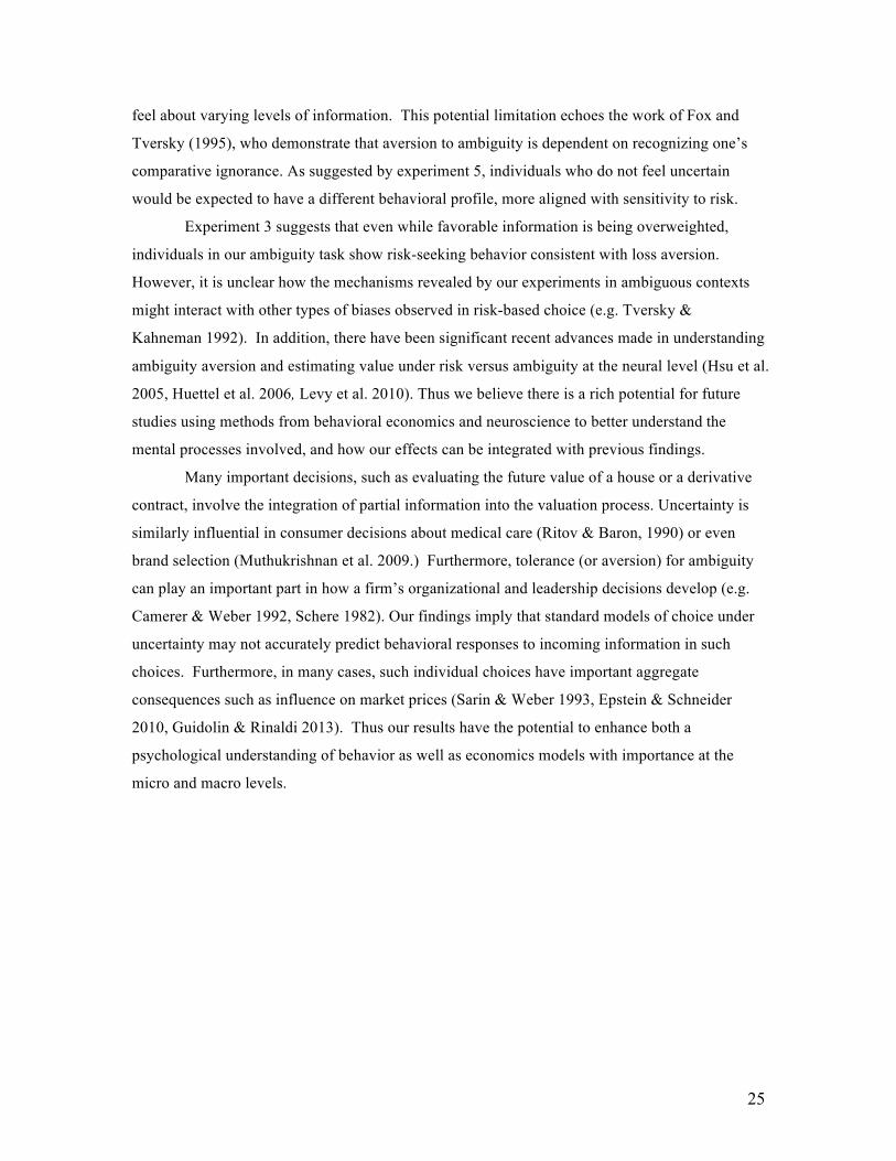
Experiment 3 suggests that even while favorable information is being overweighted,

individuals in our ambiguity task show risk-seeking behavior consistent with loss aversion.

However, it is unclear how the mechanisms revealed by our experiments in ambiguous contexts

might interact with other types of biases observed in risk-based choice (e.g. Tversky &

Kahneman 1992). In addition, there have been significant recent advances made in understanding

ambiguity aversion and estimating value under risk versus ambiguity at the neural level (Hsu et al.

2005, Huettel et al. 2006, Levy et al. 2010). Thus we believe there is a rich potential for future

studies using methods from behavioral economics and neuroscience to better understand the

mental processes involved, and how our effects can be integrated with previous findings.

Many important decisions, such as evaluating the future value of a house or a derivative

contract, involve the integration of partial information into the valuation process. Uncertainty is

similarly influential in consumer decisions about medical care (Ritov & Baron, 1990) or even

brand selection (Muthukrishnan et al. 2009.) Furthermore, tolerance (or aversion) for ambiguity

can play an important part in how a firm’s organizational and leadership decisions develop (e.g.

Camerer & Weber 1992, Schere 1982). Our findings imply that standard models of choice under

uncertainty may not accurately predict behavioral responses to incoming information in such

choices. Furthermore, in many cases, such individual choices have important aggregate

consequences such as influence on market prices (Sarin & Weber 1993, Epstein & Schneider

2010, Guidolin & Rinaldi 2013). Thus our results have the potential to enhance both a

psychological understanding of behavior as well as economics models with importance at the

micro and macro levels.

 

26

Tables

Table 1: Summary of Experimental Studies

Experiment Paradigm Incentives Favorable Information

Unfavorable Information

1 Pull-a-chip: gains

AMT (n = 100)

Hypothetical

Win = $50

# red (winning) chips

# blue (no-win) chips

2 Pull-a-chip: gains,

choice of winning color

AMT (n = 111)

Hypothetical

Win = $50

# chips of chosen (winning) color, defined on each round

# chips of unchosen (no-win) color, defined on each round

3 Pull-a-chip: losses

AMT (n = 53)

Hypothetical

Win = Retain $50 endowment

# of red (no-loss) chips

# blue (lose) chips

4A Pull-a-chip: gains

Majority : gains

In lab (n= 37)

Incentive compatible

Win = 30 points ($7)

# red (winning) chips

#blue (no-win) chips

4B Trivia : gains,

subjectively interpreted information

In lab (n = 27)

Incentive compatible

Win = 30 points ($7)

# supporting facts, as designated by participant

# contradicting facts, as designated by participant

5 Pull-a-chip: gains,

estimates of likelihood and certainty

In lab (n=29)

Incentive compatible

Win = $30

# red (winning) chips

# blue (no-win) chips

27

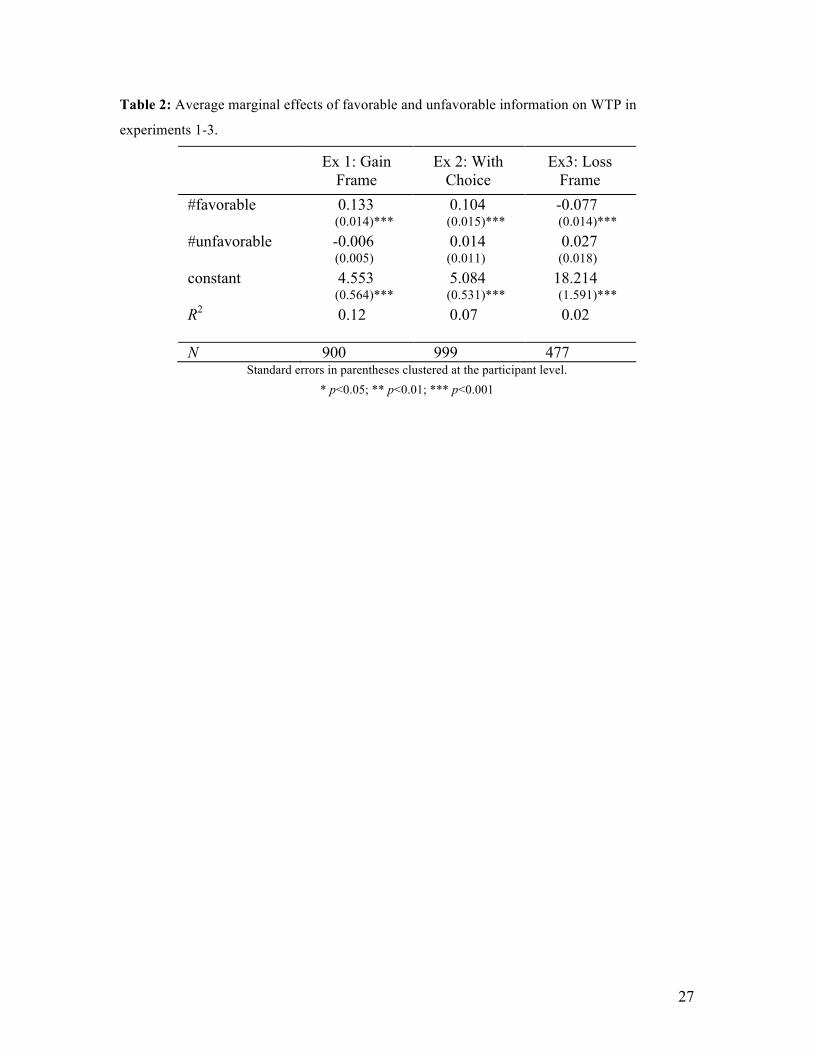
Table 2: Average marginal effects of favorable and unfavorable information on WTP in

experiments 1-3.

Ex 1: Gain Frame

Ex 2: With Choice

Ex3: Loss Frame

#favorable 0.133 0.104 -0.077 (0.014)*** (0.015)*** (0.014)*** #unfavorable -0.006 0.014 0.027 (0.005) (0.011) (0.018) constant 4.553 5.084 18.214 (0.564)*** (0.531)*** (1.591)*** R2 0.12 0.07 0.02 N 900 999 477

Standard errors in parentheses clustered at the participant level. * p<0.05; ** p<0.01; *** p<0.001

28

Table 3: Experiment 4: Average marginal effects of favorable and unfavorable information on

WTP across game types.

Pull-a-Chip Game

Majority Game

Trivia Game

#favorable 0.136 0.099 7.353 (0.015)*** (0.014)*** (1.005)*** #unfavorable -0.058 -0.012 -2.906 (0.014)*** (0.009) (0.939)** constant 6.504 6.362 7.418 (0.738)*** (0.646)*** (0.774)*** R2 0.23 0.14 0.24 N 332 333 370

Standard errors in parentheses clustered at the participant level. * p<0.05; ** p<0.01; *** p<0.001

29

Table 4: Experiment 5 Results: WTP conditional on amounts of favorable and unfavorable

information (col. 1), and when restricted to the final 25 rounds (col. 4). Willingness to purchase

conditional on amounts of favorable and unfavorable information (cols. 2 and 3).

WTP Purchase, Probit

Purchase Binary, LPM

WTP, Last 25 rounds

#favorable 0.107 0.036 0.011 0.105 (0.012)*** (0.005)*** (0.001)*** (0.014)*** #unfavorable -0.028 -0.012 -0.003 -0.024 (0.011)* (0.004)** (0.001)** (0.010)* constant 1.685 0.078 1.706 (0.491)** (0.052) (0.486)** R2 0.30 0.29 0.24 N 1,450 1,450 1,450 725

Standard errors in parentheses clustered at the participant level. * p<0.05; ** p<0.01; *** p<0.001

30

Table 5: Experiment 5 Likelihood of a winning outcome and felt certainty increase willingness

to pay as well as willingness to purchase decisions.

WTP Purchase (Probit)

Purchase Binary (LPM)

likelihood 1.523 0.559 0.176 (0.177)*** (0.066)*** (0.013)*** certainty 0.452 0.108 0.049 (0.126)** (0.042)** (0.012)*** constant 2.053 0.107 (0.720)** (0.075) R2 0.31 0.35 N 1,450 1,450 1,428

Standard errors in parentheses clustered at the participant level. * p<0.05; ** p<0.01; *** p<0.001

31

Table 6: The impact of information on estimated likelihood is directional dependent on valence.

However, both favorable and unfavorable information increase felt certainty. Coefficients from

ordered Probit regressions.

Likelihood

Red Certainty

numred 0.043 0.024 (0.008)*** (0.003)*** numblue -0.045 0.029 (0.008)*** (0.003)*** N 2,900 2,900

Standard errors in parentheses clustered at the participant level. * p<0.05; ** p<0.01; *** p<0.001

32

Figure  1:  Experiment  1  WTP  for  pull-­‐a-­‐chip  games  with  partial  information.  The  effect  of  

incrementing  favorable  information  (seen  in  the  differing  colors)  is  significantly  larger  than  

the  effect  of  incrementing  unfavorable  information.  

   

     

0 25

50

0

2

4

6

8

10

12

14

0 25 50

# Unfavorable Chips

# Favorable

Chips

33

Figure  2:  Experiment  4b.  A)  Example  of  trivia  game  round  with  two  facts  present.  B)  WTP  for  trivia  games  by  subjectively  reported  information  conditions.    

 

   

TRIVIA 1

This ticket is worth 30 Points if the following is true:

According to the Old Farmer’s Almanac, the high temperature in San Diego, California on April 28,

2010 was ABOVE 66 degrees.

FACT: According to the Old Farmer’s Almanac, since the 1970’s the average high temperature in April in San

Diego, CA was 68 degrees.

FACT: According to the Old Farmer’s Almanac, the high temperature in San Diego on April 26, 2010 (two days

before) was 62.6 degrees.

B

A

34

Figure  3:  Channels  by  which  information  affects  willingness  to  pay  for  AFPs.  

Favorable Info

Unfavorable Info

Estimated Likelihood

Subjective Certainty

WTP

35

Figure 4: Experiment 5 Mean WTP across randomly generated AFPs. X-axis shows the amount of favorable information (# chips of the winning color) with lines disaggregated into rounds with high or low amount of unfavorable information. Lines are locally estimated regressions with shaded 95% confidence intervals.

!

!

!

!

!

!

!

!

!

!

!

!

!

!

!!

!

!

!

!!

!

!

!

!

!!

!

!

!

!

!

!

!

!

!

!

!

!

!

!

!

!

!

!

!

!

!

!

!

!

!

!

!

!

!

!

!

!

!

!

!

!

!

!

0

3

6

9

0 20 40 60Favorable

Mea

n W

TP

Unfavorable Info ! !High Low

36

Figure 5: Experiment 5 A. Positive effect of estimated likelihood of a good outcome on WTP. B. Positive effect of subjective certainty on WTP. Error bars represent unclustered standard errors.

Mea

n W

TPM

ean

WTP

12

8

4

0

Likelihood Rating0 2-2-4

Subjective Certainty Rating7.55.02.5

3

5

4

A

B

37

References Amir, O., Rand, DG & Gal, K. (2012). "Economic games on the internet: The effect of $1 stakes." PLoS One 7(2). Baumeister, R., Bratslavsky, E, Finkenauer, C & Vohs, K (2001). "Bad is stronger than good." Review of General Psychology 5(4): 1089-2056. Becker, G., Degroot, M & Marschack, J (1964). "Measuring utility by a single response sequential method." Behavioral Science 9(3): 226-232. Bushong, B., King, L., Camerer, C. & Rangel A. (2010). "Pavlovian processes in consumer choice: The physical presence of a good increases willingness-to-pay." American Economic Review 100(4): 1556-1571. Camerer, C. & Weber, M. (1992). "Recent developments in modeling preferences: uncertainty and ambiguity." Journal of Risk and Uncertainty 5(4): 325-370. Camerer, C. (1995). Individual decision-making. The Handbook of Experimental Economics. Eds. Kagel, J. & Roth, A.. Princeton, Princeton University Press. 1: 587-683. Charness, G. & Gneezy, U (2010). "Portfolio choice and risk attitudes: an experiment." Economic Inquiry 48(1): 133-146. Eil, D. & Rao J. (2012). "The good news-bad news effect: asymmetric processing of information about yourself." AEJ: Microeconomics 3(2): 114-138. Ellsberg, D. (1961). "Risk, Ambiguity, and the Savage Axioms” Quarterly Journal of Economics 100(3): 585-603. Epstein, L., & Schneider, M. (2010). “Ambiguity and asset markets.” Annual Review of Financial Economics, Annual Reviews, vol. 2(1), pages 315-346 Fox, C. & Tversky, A (1995). "Ambiguity aversion and comparative ignorance." Quarterly Journal of Economics 100(3): 585-603. Frisch, D. B. J. & Baron, J. (1988). "Ambiguity and rationality." Journal of Behavioral Decision Making 1(3): 149-157. Fudenberg, D. & Peysakhovich, A. (2014) "Recency, records and recaps: non-equilibrium behavior in a simple decision problem" Proceedings of the ACM 15th Annual Conference on Economics and Computation Gilboa, I. & Schmeidler, D. (1989). "Maxmin expected utility with non-unique prior." Journal of Mathematical Economics 18(2): 141-153. Grant, S., Polak, B. & Strzalecki, T. (2009) “Second-order expected utility.” Working paper Guidolin, M., & Rinaldi, F. (2013). "Ambiguity in asset pricing and portfolio choice: a review of the literature." Theory and Decision 74(2): 183-217.

38

Gul, F., & Pesendorfer, W. (2014). “Expected uncertain utility theory.” Econometrica, 82(1), 1-39. Halevy, Y. (2007). "Ellsberg revisited: An experimental study." Econometrica 75(2): 503-536. Hsu, M., Bhatt, M, Adolphs, R, Tranel, D & Camerer, C.F. (2005). "Neural systems responding to degrees of uncertainty in human decision-making." Science 310(5754): 1680-1683. Huettel, S., Stowe C., Gordon, E., Warner, B. & Platt M.L. (2006). "Neural signatures of economic preferences for risk and ambiguity." Neuron 49(5): 765-777. Imas, A. (2014) “The Realization Effect: Risk Taking After Realized Versus Paper Losses” Available at SSRN 2403865. Jain, S. & Maherswaran D. (2000). "Motivated reasoning: a depth-of-processing perspective." Journal of Consumer Research 26(4): 358-371. Johnson, E. J., Häubl, G., & Keinan, A. (2007). “Aspects of endowment: a query theory of value construction.” Journal of Experimental Psychology: Learning, Memory, and Cognition, 33(3), 461. Kahneman, D. & Tversky, A (1979). "Prospect theory: an analysis of choice under risk." Econometrica 47(2): 263-291. Kahneman, D. & Tversky, A Eds. (2000). Choices, Values and Frames. Cambridge, UK, Cambridge University Press. Kang, M. J., Rangel, A., Camus, M., & Camerer, C. F. (2011). Hypothetical and real choice differentially activate common valuation areas. The Journal of Neuroscience, 31(2), 461-468. Klibanoff, P., Marinacci, M., & Mukerji, S. (2005). A smooth model of decision making under ambiguity. Econometrica, 73(6), 1849-1892. Kreps, D. (1988). Notes on the Theory of Choice. Boulder, Westview Press. Levy, I., Snell, J, Nelson, A, Rustichini, A & Glimcher, P (2010). "Neural representation of subjective value under risk and ambiguity." Journal of Neurophysiology 103(2): 1036-1047. Lord, C., Ross, L & Lepper, M (1979). "Biased assimilation and attitude polarization: the effect of prior theories on subsequently considered evidence." Journal of Personality and Social Psychology 37(11): 2098-2109. Maafi, H. (2011). Preference reversals under ambiguity. Management Science, 57(11), 2054-2066. Maccheroni, F., Marinacci, M & Rustichini, A (2006). "Ambiguity aversion, robustness and the variational representation of preferences." Econometrica 74(6): 1447-1498. Muthukrishnan, A., Wathieu, L & Xu, A (2009). "Ambiguity aversion and the preference for established brands." Management Science 55(12): 1933-1941.

39

Oechssler, J. & Roomets, A. (2013) “A Test of Mechanical Ambiguity” Working Papers, University of Heidelberg, Department of Economics 0555. Paolacci, G., & Chandler, J. (2014). “Inside the Turk Understanding Mechanical Turk as a Participant Pool.” Current Directions in Psychological Science, 23(3), 184-188. Peeters, G. & Czapinski, J (1990). "Positive-negative asymmetry in evaluations: The distinction between affective and informational negativity effects." European Review of Social Psychology 1(1): 33-60. Rand, D. G., Peysakhovich, A., Kraft-Todd, G. T., Newman, G. E., Wurzbacher, O., Nowak, M. A., & Greene, J. D. (2014). “Social heuristics shape intuitive cooperation.” Nature communications, 5. Ritov, I. & Baron J. (1990). "Reluctance to vaccinate: omission bias and ambiguity." Journal of Behavioral Decision Making 3(4): 263-277. Rozin, P. & Royzman E. (2006). "Negativity bias, negativity dominance and contagion." Personality and Social Psychology Review 5(2): 296-320. Russo, J., Medvec, V & Meloy M (2004). "The distortion of information during decisions." Organizational Behavior and Human Decision Processes 66(1): 102-110. Sarin, R. & Weber, M (1993). "Effects of ambiguity in market experiments." Management Science 39(5): 602-615. Savage, L. (1972). Foundation of Statistics, Courier Dover Publications. Segal, U. (1987). “The Ellsberg paradox and risk aversion: An anticipated utility approach.” International Economic Review, 175-202. Schere, J. (1982). “Tolerance of ambiguity as a discriminating variable between entrepreneurs and managers.” Academy of Management Proceedings (1): 404-408. Shafir, E. (1994). “Uncertainty and the difficulty of thinking through disjunctions”. Cognition, 50(1), 403-430. Sharot, T., Kanai, R, Marston, D, Korn, C, Rees, G & Dolan R (2012). "Selectively altering belief formation in the human brain." Proceedings of the National Academy of Sciences 109(42): 17058-17062. Trautmann, S. T., & van de Kuilen, G. (2013). "Ambiguity Attitudes." Handbook of Judgment and Decision Making. Trautmann, S. T., Vieider, F. M., & Wakker, P. P. (2011). “Preference reversals for ambiguity aversion” Management Science, 57(7), 1320-1333. Tversky, A. & Fox, C (1995). "Weighting risk and uncertainty." Psychological Review 102(2): 269-282. Tversky, A., & Kahneman, D. (1992). “Advances in prospect theory: Cumulative representation of uncertainty.” Journal of Risk and Uncertainty, 5(4), 297-323. Tversky, A., & Shafir, E. (1992). “The disjunction effect in choice under uncertainty.” Psychological

40

Science, 3(5), 305-309. Tymula, A., Rosenberg, L., Roy, A., Ruderman, L., Manson, K., Glimcher, P. & Levy, I. (2012). "Adolescents' risk-taking behavior is driven by tolerance to ambiguity." Proceedings of the National Academy of Sciences 109(42): 17135-17140. Wason, P. (1966). Reasoning. New horizons in psychology. B. Foss. England, Penguin Press. Weber, E. U., Johnson, E. J., Milch, K. F., Chang, H., Brodscholl, J. C., & Goldstein, D. G. (2007). “Asymmetric discounting in intertemporal choice a query-theory account.” Psychological Science, 18(6), 516-523. Westen, D., Blagov, P., Harenski, K., Kilts, C. & Hamann S. (2006). "Neural basis of motivated reasoning: an fMRI study of emotional constraints on partisan political judgment in the 2004 US presidential election." Journal of Cognitive Neuroscience 18(11): 1947-1958.