Astron. Astrophys. 356, 490–500 (2000) ASTRONOMYAND

ASTROPHYSICS

Eclipse mapping of the accretion stream in UZ Fornacis?

J. Kube, B.T. Gansicke, and K. Beuermann

Universitats-Sternwarte Gottingen, Geismar Landstrasse 11, 37083 Gottingen, Germany

Received 4 August 1999 / Accepted 17 December 1999

Abstract. We present a new method to map the surface bright-ness of the accretion streams in AM Herculis systems from ob-served light curves. Extensive tests of the algorithm show thatit reliably reproduces the intensity distribution of the stream fordata with a signal-to-noise ratio>∼ 5. As a first application, wemap the accretion stream emission of Civ λ 1550 in the polarUZ Fornacis using HST FOS high state spectra. We find threemain emission regions along the accretion stream: (1) On theballistic part of the accretion stream, (2) on the magneticallyfunneled stream near the primary accretion spot, and (3) on themagnetically funneled stream at a position above the stagnationregion.

Key words: accretion, accretion disks – methods: data analy-sis – stars: binaries: close – stars: binaries: eclipsing – stars:individual: UZ For – stars: novae, cataclysmic variables

1. Introduction

Polars, as AM Hers are commonly named due to their highlypolarized emission, consist of a late type main-sequence star(red dwarf, secondary star) and a highly magnetized white dwarf(WD, primary star). The red dwarf, filling its Roche volume,injects matter through theL1 point into the Roche volume ofthe WD. Unlike in non-magnetic systems, this material doesnot form an accretion disc, but couples onto the magnetic fieldonce the magnetic pressure exceeds the ram pressure. Fromthis stagnation region (SR) on, the accretion stream follows amagnetic field line until it impacts onto the white dwarf surface.For a review of polars, see Warner (1995).

In systems with an inclinationi >∼ 70◦, the secondary stargradually eclipses the accretion stream during the inferior con-junction. Using tomographical methods, it is – in principle –possible to reconstruct the surface brightness distribution on theaccretion stream from time resolved observations. This method

Send offprint requests to: Jens Kube (jkube@uni-goettingen.de)? The observational part of this work is based on observations made

with the NASA/ESA Hubble Space Telescope, obtained from the dataArchive at the Space Telescope Science Institute, which is operated bythe Association of Universities for Research in Astronomy, Inc., underNASA contract NAS 5-26555. These observations are associated withproposal ID 4013.

has been successfully applied to accretion discs in non-magneticCVs (“eclipse mapping”, Horne 1985). We present tests and afirst application of a new eclipse mapping code, which allowsthe reconstruction of the intensity distribution on the accretionstream in magnetic CVs.

Similar attempts to map accretion streams in po-lars have been investigated by Hakala (1995) andVrielmann & Schwope (1999) for HU Aquarii. An im-proved version of Hakala’s 1995 method has been presentedby Harrop-Allin et al. (1999b) with application to real datafor the system HU Aquarii (Harrop-Allin et al. 1999a). Adrawback of all these approaches is that they only considerthe eclipse of the accretion stream by the secondary star. Inreality, the geometry may be more complicated: the far side ofthe magnetically coupled stream may eclipse stream elementsclose to the WD as well as the hot accretion spot on the WDitself. The latter effect is commonly observed as a dip in thesoft X-ray light curves prior to the eclipse (e.g. Sirk & Howell1998). The stream-stream eclipse may be detected in datawhich are dominated by emission from the accretion stream,e.g. in the light curves of high-excitation emission lines wherethe secondary contributes only little to the line flux.

Here, we describe a new accretion stream eclipse mappingmethod, using a 3d code which can handle the full complexity ofthe geometry together with an evolution strategy as fit algorithm.We present extensive tests of the method and map as a firstapplication to real data the accretion stream in UZ For emissionof C iv λ 1550.

2. The 3d cataclysmic variable model

Our computer code CVMOD generatesN small surface ele-ments (convex quadrangles, some of which are degenerated totriangles), which represent the surfaces of the individual com-ponents of the CV (WD, secondary, accretion stream) in three-dimensional space (Fig. 1). Using simple rotation algorithms,the position of each surface elementi = 1 . . . N can be com-puted for a given orbital phaseΦ.

The white dwarf is modelled as an approximatedsphere, using surface elements of nearly constant area(Gansicke et al. 1998). Thesecondary staris assumed to fillits Roche volume. Here, the surface elements are choosen insuch a way that their boundaries align with longitude and lat-

J. Kube et al.: Eclipse mapping of the accretion stream in UZ Fornacis 491

itude circles of the Roche surface, taking theL1-point as theorigin.

We generate the surface of theaccretion streamin two parts,(a) the ballistic part fromL1 toSR, and (b) the dipole-part fromSR to the surface of the white dwarf.

(a) For the ballistic part of the stream, we use single-particletrajectories. The equations of motion in the corotating frame aregiven by

x = +µx − x1

r31

− (1 − µ)x − x2

r32

+ 2y + x (1)

y = −µy

r31

− (1 − µ)y

r32

− 2x + y (2)

z = −µz

r31

− (1 − µ)z

r32

(3)

Eq. (3) has been added to Flannery’s 1975 set of two-dimensional equations.µ = (M1+M2)/M1 is the mass fractionof the white dwarf,r1 andr2 are the distances from the point(x, y, z) to the white dwarf and the secondary, respectively, inunits of the orbital separationa. The coordinate origin is at thecentre of gravity, thex-axis is along the lines connecting the cen-tres of the stars, the system rotates with the angular frequencyω around to thez-axis. The velocityv = (x, y, z) is given inunits ofaω, v0 = (x0, y0, z0) is the initial velocity in theL1point.

If z0 = 0, the trajectories resulting from the numerical inte-gration of Eqs. (1) – (3) are restricted to the orbital plane. How-ever, calculating single-particle trajectories with different initialvelocity directions (allowing alsoz0 /= 0) shows that there is aregion approximately one third of the way downstream fromL1to SR where all trajectories pass within very small separations,corresponding to a striction of the accretion stream.

We define a 3d version of the stream as a tube with a circularcross section with radiusrTube = 5 × 108 cm centred on thesingle-particle trajectory forx = 10 km s−1, y = z = 0.

(b) When the matter reachesSR, we switch from a ballisticsingle-particle trajectory to a magnetically forced dipole geom-etry. The central trajectory is generated using the dipole formular = r0 sin2 α, whereα is the angle between the dipole axis andthe position of the particle(r, ϕ, α). This can be interpreted asthe magnetic field lineF passing through the stagnation pointSR and the hot spots on the WD. KnowingF , we assume a cir-cular cross section with the radiusrSR = rTube = 5 × 108 cmfor the region where the dipole intersects the ballistic stream.This cross section is subject to transformation asα changes.Thus, the cross section of the stream is no longer constant inspace but bounded everywhere by the same magnetic field lines.

Our accretion stream model involves several assumptions:(1) The cross section of the stream itself is to some extent ar-bitrary because we consider it to be – for our current data, seebelow – essentially a line source. (2) The neglect of the magneticdrag (King 1993; Wynn & King 1995) on the ballistic part of thestream and the neglect of deformation of the dipole field causethe model stream to deviate in space from the true stream trajec-tory. While, in fact, the location ofSR may fluctuate with ac-cretion rate (as does the location of the Earth’s magnetopause),

1L SR

Fig. 1. Overview of our 3d-Model of a polar.L1 marks the inner la-grangian point,SR the position of the stagnation or coupling region.

the evidence for a sharp soft X-ray absorption dip caused by thestream suggest thatSR does not wander about on time scalesshort compared to the orbital period. (3) The abrupt switch-overfrom the ballistic to the dipole part of the stream may not de-scribe the physics ofSR correctly. This discrepancy, however,does not seriously affect our results, because the eclipse tomog-raphy is sensitive primarily to displacements in the times ofingress and egress ofSR which are constrained by the absorp-tion dip in the UV continuum (and, in principle, in soft X-rays).The≈ 5 sec time bins of our observed light curves correspondto ≈ 108 cm in space atSR. Hence, our code is insensitive tostructure on a smaller scale. In fact, the smallest resolved struc-tures are much larger because of the noise level of our data.While our approach clearly involves several approximations, itis tailored to the desired aim of mapping the accretion streamfrom the information obtained from an emission line light curve.

In our current code, we restrict the possible brightness dis-tribution so that for each stream segment, which consists of 16surface elements forming a section of the tube-like stream, theintensity is the same, i.e. there is no intensity variation around thestream. For the current data, this is no serious drawback, sincewe only use observations covering a small phase interval aroundthe eclipse. Our results refer, therefore, to the stream brightnessas seen from the secondary. From the present observations wecan not infer how the fraction of the stream illuminated by theX-ray/UV spot on the WD looks like. The required extensionof our computer code, allowing for brightness variation aroundthe stream, is straightforward. The present version of the codeis, however, adapted to the data set considered here.

3. Light curve fitting

The basic idea of our eclipse mapping algorithm is to recon-struct the intensity distribution on the accretion stream by com-paring and fitting a synthetic light curve to an observed one.The comparison between these light curves is done with aχ2-minimization, which is modified by means of a maximum en-tropy method. Sect. 3.1 describes the light curve generation, 3.2the maximum entropy method, and 3.3 the actual fitting algo-rithm.

3.1. Light curve generation

In order to generate a light curve from the 3d model, it is nec-cessary to know which surface elementsi are visible at a givenphaseΦ. We designate theset of visible surfacesV (Φ).

492 J. Kube et al.: Eclipse mapping of the accretion stream in UZ Fornacis

In general, each of the three components (WD, secondary,accretion stream) may eclipse (parts of) the other two, and theaccretion stream may partially eclipse itself. This is a typicalhidden surface problem. However, in contrast to the widespreadcomputer graphics algorithms which work in the image spaceof the selected output device (e.g. a screen or a printer), andwhich provide the information ‘pixelj shows surfacei’, weneed to work in the object space, answering the question ‘issurfacei visible at phaseΦ?’. For a recent review on objectspace algorithms see Dorward (1994). Unfortunately, there isno readily available algorithm which fits our needs, thus weuse a self-designed 3d object-space hidden-surface algorithm.Let N be the number of surface elements of our 3d model.According to Dorward (1994), the timeT needed to perform anobject space visibility analysis goes likeT ∝ N log N . . . N2.Our algorithm performs its task inT ∝ N1.5...1.8, with thefaster results during the eclipse of the system. It is obviouslynecessary to optimize the number of surface elements in orderto minimize the computation time without getting too coarse a3d grid.

OnceV (Φ) has been determined, the angles between thesurface normals ofi ∈ V (Φ) and the line of sight, and theprojected areasAi,Φ of i ∈ V (Φ) are computed. Designatingthe intensity of the surface elementi at the wavelengthλ withIi,λ, the observed fluxFλ(Φ) is

Fλ(Φ) =∑

i∈V (Φ)

Ii,λAi(Φ) (4)

Here, two important assumptions are made: (a) the emissionfrom all surface elements is optically thick, and (b) the emissionis isotropic, i.e. there is no limb darkening in addition to theforeshortening of the projected area of the surface elements.The computation of a synthetic light curve is straightforward. Itsuffices to computeFλ(Φ) for the desired set of orbital phases.

While the above mentioned algorithm can produce lightcurves for all three components, the WD, the secondary, andthe accretion stream, we constrain in the following the com-putations of light curves to emission from the accretion streamonly. Therefore, we treat the white dwarf and the secondary staras dark opaque objects, screening the accretion stream.

3.2. Constraining the problem: MEM

In the eclipse mapping analysis, the number of free parameters,i.e. the intensity of theN surface elements, is typically muchlarger than the number of observed data points. Therefore, onehas to reduce the degrees of freedom in the fit algorithm in a sen-sible way. An approach which has proved successful for accre-tion discs is the maximum entropy method MEM (Horne 1985).The basic idea is to define an image entropyS which has to bemaximized, while the deviation between synthetic and observed

light curve, usually measured byχ2/n, is minimized (n is thenumber of phase steps or data points). LetDi be

Di =

N∑j=1

Ij exp(

− (ri − rj)2

2∆2

)

N∑j=1

exp(

− (ri − rj)2

2∆2

) (5)

the default image for the surface elementi. Then the entropy isgiven by

S =

N∑i=1

Ii

(ln

Ii

Di− 1

)

N∑i=1

Ii

(6)

In Eq. (5),ri andrj are the positions of the surface elementsiandj. ∆ determines the range of the MEM in that the defaultimage (5) is a convolution of the actual image with a Gaus-sian with theσ-width of ∆. Hence, the entropy measures thedeviation of the actual image from the default image. An idealentropic image (with no contrast at all) hasS = 1. We use∆ = 1 × 109 cm ≈ 0.02a for our test calculations and for theapplication to UZ For.

The quality of a intensity map is given as

Q = χ2/n − λS, (7)

whereλ is chosen in the order of 1. Aim of the fit algorithm isto minimizeQ.

3.3. The fitting algorithm: evolution strategy

Our model involves approximately 250 parameters, which arethe intensities of the surface elements. This large number isnotthe number of the degrees of freedom, which is difficult to de-fine in a MEM-strategy. A suitable method to find a parameteroptimum with a leastχ2 and a maximum entropy value is a sim-plified imitiation of biological evolution, commonly referred toas ‘evolution strategy’ (Rechenberg 1994). The intensity infor-mation of thei surface elements is stored in the intensity vectorI. Initially, we chooseIi = 1 for all i.

From this parent intensity map, a number of offsprings arecreated withIi randomly changed by a small amount, the so-calledmutation. For all offsprings, the qualityQ is calculated.The best offspring is selected to be the parent of the next gener-ation. An important feature of the evolution strategy is that theamount of mutation itself is also being evolved just as if it werepart of the parameter vector. We use the C-program library evoCdeveloped by K. Trint and U. Utecht from the Technische Uni-versitat Berlin, which handles all the important steps (offspringgeneration, selection, stepwidth control).

In contrast to the classical maximum entropy optimisation(Skilling & Bryan 1984), the evolution strategy does not offer aquality parameter that indicates how close the best-fit solutionis to the global optimum. In order to test the stability of ourmethod, we run the fit several times starting from randomly

J. Kube et al.: Eclipse mapping of the accretion stream in UZ Fornacis 493

Table 1.System geometry of the imaginary system IM Sys

mass ratio Q = M1/M2 = 4total mass M = M1 + M2 = 0.9M�orbital period P = 100 mininclination i = 88◦

dipole tilt β = 20◦

dipole azimuth Ψ = 35◦

angle toSR ΨS = 35◦

distributed maps. All runs converge to very similar intensitydistributionsI (see also Figs. 10 and 12). This type of test iscommon in evolution strategy or genetic algorithms (e.g. Hakala1995). Even though this approach is not a statistically ‘clean’test, it leaves us to conclude that we find the global optimum.

Fastest convergence is achieved with 40 to 100 offsprings ineach generation. Finding a good fit (χ2/n) takes only on tenth toone fifth of the total computation time, the remaining iterationsare needed to improve the smoothness of the intensity map, i.e.to maximizeS. A hybrid code using a classical optimization al-gorithm, e.g. Powell’s method, may speed up the regularization(Potter et al. 1998).

4. Tests

To test the quality and the limits of our method, we producesynthetical test light curves with different noise levels (S/N=∞, 50, 20, 10, 4). We then try to reproduce our initial intensitydistribution on the stream from the synthetic data. Two testswith different intensity distributions are performed. For bothtests, the geometry of the imaginary system IM Sys is chosen asshown in Table 1. The phase coverage isΦ = 0.865 . . . 1.070with 308 equidistant steps, which is identical to the real HSTdata of UZ For which we use below for a first application.

Additionally, we test our algorithm with a full-orbit lightcurve with S/N= 10 to demonstrate its capabilities if more thanjust the ingress information for each stream section is available.

4.1. One bright region nearSR

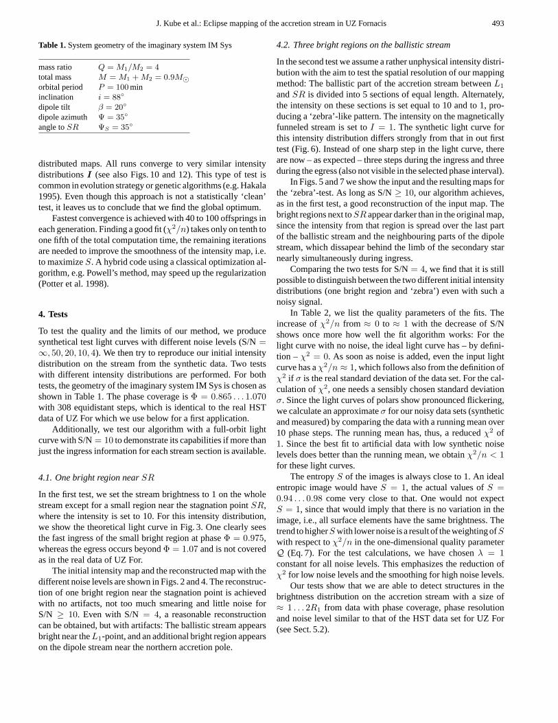
In the first test, we set the stream brightness to 1 on the wholestream except for a small region near the stagnation pointSR,where the intensity is set to 10. For this intensity distribution,we show the theoretical light curve in Fig. 3. One clearly seesthe fast ingress of the small bright region at phaseΦ = 0.975,whereas the egress occurs beyondΦ = 1.07 and is not coveredas in the real data of UZ For.

The initial intensity map and the reconstructed map with thedifferent noise levels are shown in Figs. 2 and 4. The reconstruc-tion of one bright region near the stagnation point is achievedwith no artifacts, not too much smearing and little noise forS/N ≥ 10. Even with S/N= 4, a reasonable reconstructioncan be obtained, but with artifacts: The ballistic stream appearsbright near theL1-point, and an additional bright region appearson the dipole stream near the northern accretion pole.

4.2. Three bright regions on the ballistic stream

In the second test we assume a rather unphysical intensity distri-bution with the aim to test the spatial resolution of our mappingmethod: The ballistic part of the accretion stream betweenL1andSR is divided into 5 sections of equal length. Alternately,the intensity on these sections is set equal to 10 and to 1, pro-ducing a ‘zebra’-like pattern. The intensity on the magneticallyfunneled stream is set toI = 1. The synthetic light curve forthis intensity distribution differs strongly from that in out firsttest (Fig. 6). Instead of one sharp step in the light curve, thereare now – as expected – three steps during the ingress and threeduring the egress (also not visible in the selected phase interval).

In Figs. 5 and 7 we show the input and the resulting maps forthe ‘zebra’-test. As long as S/N≥ 10, our algorithm achieves,as in the first test, a good reconstruction of the input map. Thebright regions next toSR appear darker than in the original map,since the intensity from that region is spread over the last partof the ballistic stream and the neighbouring parts of the dipolestream, which dissapear behind the limb of the secondary starnearly simultaneously during ingress.

Comparing the two tests for S/N= 4, we find that it is stillpossible to distinguish between the two different initial intensitydistributions (one bright region and ‘zebra’) even with such anoisy signal.

In Table 2, we list the quality parameters of the fits. Theincrease ofχ2/n from ≈ 0 to ≈ 1 with the decrease of S/Nshows once more how well the fit algorithm works: For thelight curve with no noise, the ideal light curve has – by defini-tion – χ2 = 0. As soon as noise is added, even the input lightcurve has aχ2/n ≈ 1, which follows also from the definition ofχ2 if σ is the real standard deviation of the data set. For the cal-culation ofχ2, one needs a sensibly chosen standard deviationσ. Since the light curves of polars show pronounced flickering,we calculate an approximateσ for our noisy data sets (syntheticand measured) by comparing the data with a running mean over10 phase steps. The running mean has, thus, a reducedχ2 of1. Since the best fit to artificial data with low synthetic noiselevels does better than the running mean, we obtainχ2/n < 1for these light curves.

The entropyS of the images is always close to 1. An idealentropic image would haveS = 1, the actual values ofS =0.94 . . . 0.98 come very close to that. One would not expectS = 1, since that would imply that there is no variation in theimage, i.e., all surface elements have the same brightness. Thetrend to higherS with lower noise is a result of the weighting ofSwith respect toχ2/n in the one-dimensional quality parameterQ (Eq. 7). For the test calculations, we have chosenλ = 1constant for all noise levels. This emphasizes the reduction ofχ2 for low noise levels and the smoothing for high noise levels.

Our tests show that we are able to detect structures in thebrightness distribution on the accretion stream with a size of≈ 1 . . . 2R1 from data with phase coverage, phase resolutionand noise level similar to that of the HST data set for UZ For(see Sect. 5.2).

494 J. Kube et al.: Eclipse mapping of the accretion stream in UZ Fornacis

Fig. 2. Maps of the synthetic stream and its reconstructions. From topto bottom: Input data, reconstructions with S/N= 50, 10, 4.

Table 2.Quality of the test calculations

S/N χ2/n S χ2/n S

bright region nearSR three bright regions∞ 0.015 0.982 0.018 0.93850 0.173 0.947 0.284 0.96020 0.593 0.968 0.668 0.95310 0.886 0.971 0.924 0.9834 1.038 0.980 1.038 0.984

4.3. Full-orbit light curve

To test the capabilities of our algorithm for data with wider phasecoverage, we fit a synthetic light curve covering the whole bi-nary orbit, computed using the same input map and geometryas in Sect. 4.1. We choose a phase resolution of 0.005 for thesimulated data, corresponding to a 30 sec time resolution, andS/N=10. The result of this fit is shown in Fig. 8. Obviously, theadditional phase information helps in producing a reliable re-construction of the initial intensity distribution, which one cansee by comparing the map in Fig. 8 with the S/N= 10-map inFig. 2. The full-orbit light curve has less phase steps than theingress-only map, but shows the same quality of the reconstruc-tion. On the other hand, the similarity between the two resultsallows us to conclude that we can rely on the reconstructions ofour algorithm even if only ingress data is available, as will be

Fig. 3. Synthetic light curve of an accretion stream which is brightaround the stagnation region. Different levels of artifical noise areadded: S/N= 50, 10, 4. The reconstructed light curves are shown assolid lines. The residuals are normalized so that the standard deviationσ is 0.1 in the relative flux units.

Fig. 4. Plot of the reconstruction of the synthetic stream with a brightregion aroundSR. Solid line: Input distribution, dotted line: recon-struction with S/N= 50, dashed line: reconstruction with S/N= 10.In the left panels (surface elements no. 0 to 104), the intensities of thesurface elements on the ballistic stream are shown. In the upper rightpanel, the northern magnetic stream is to be found (surface elementsno. 105 to 182), in the lower right panel the southern magnetic stream(surface elements no. 183 to 227).

J. Kube et al.: Eclipse mapping of the accretion stream in UZ Fornacis 495

Fig. 5. Maps of the synthetic stream and its reconstructions. From topto bottom: Input data, reconstructions withS/N = 50, 10, 4.

the case for the HST archive data of UZ For which we use inthe following.

The synthetic light curve over the full orbit shows variouseclipse and projection features, which are described in detail byKube et al. (1999).

5. Application: UZ For

5.1. System geometry of UZ For

UZ For has been identified as a polar in 1988(Berriman & Smith 1988; Beuermann et al. 1988;Osborne et al. 1988). Cyclotron radiation from a regionwith B = 53 MG has been reported by Schwope et al. (1990)and Rousseau et al. (1996). The first mass estimates forthe WD were rather high,M1 = 1.09 ± 0.01M� andM1 > 0.93M� (Hameury et al. 1988; Beuermann et al. 1988),but Bailey & Cropper (1991) and Schwope et al. (1997) de-rived significantly smaller masses,0.61M� < M1 < 0.79M�and M1 = 0.75M�, respectively. We use reliable systemparameters from Bailey & Cropper (1991),q = M1/M2 = 5,M = M1 + M2 = 0.85 M�, i = 81◦, P = 126.5 min.The optical light curve in Bailey (1995) shows two eclipsesteps which are interpreted as the signature of hot spots nearboth magnetic poles of the WD, consecutively dissapearingbehind the limb of the secondary star. From that light curvewe measure the timing of the eclipse events with an accuracy

Fig. 6. Synthetic light curve of an accretion stream with three brightparts on the ballistic stream. Different levels of artifical noise are added:S/N = 50, 10, 4. The reconstructed light curves are shown as solidlines. The residuals are normalized so that the standard deviationσ isat 0.1 in the relative flux.

Fig. 7. Plot of the reconstruction of the synthetic stream with threebright regions on the ballistic stream. Solid line: Input distribution,dotted line: reconstruction with S/N= 50, dashed line: reconstructionwith S/N = 10. For an explanation of the plot see Fig. 4

of ∆Φ = 5 · 10−4. The ingress of the spot on the lowerhemisphere occurs atΦ = 0.9685, its egress atΦ = 1.0310.

496 J. Kube et al.: Eclipse mapping of the accretion stream in UZ Fornacis

Fig. 8. Top: Full-orbit reconstruction of the ‘point’-brightness distri-bution. Compare to Fig. 2, top. Bottom: Full-orbit synthetic light curveand best-fit light curve. For clarity, two full orbits are shown.

For the spot on the upper hemisphere, ingress is atΦ = 0.9725and egress atΦ = 1.0260.

To describe the spatial position of the dipole field line alongwhich the matter is accreted, three angles are needed: The co-latitude or tilt of the dipole axisβ, the longitude of the dipoleaxis Ψ, and the longitude of the stagnation regionΨS . Here,longitude is the angle between the secondary star and the re-spective point as seen from the centre of the white dwarf. Withour choice ofβ, Ψ, andΨS , we can reproduce the ingress andegress of the two hot spots as well as the dip at phaseΦ = 0.9.A summary of the main system parameters used in this analysisis given in Table 3.

Having the correct geometry of the accretion stream is cru-cial for generating the correct reconstruction of the emissionregions. As we have shown in Kube et al. (1999) especially thegeometry of the dipole stream is sensitive to changes inΨ, ΨS ,andβ. For UZ For, the geometry of the dipole stream is rel-atively well constrained from the observed ingress and egressof both hot spots on the white dwarf (Bailey 1995). Fitting theUZ For light curves system geometries that differ within theestimated error range of less than five degrees does, however,not significantly affect our results. This situation is different ifthe errors in the geometry parameters are larger than only a fewdegrees.

5.2. Observational data

UZ For was observed with HST on June 11, 1992. A detaileddescription of the data is given by Stockman & Schmidt (1996).We summarize here only the relevant points.

Fig. 9. Trailed spectrum of UZ For, both observed orbits added andrebinned. The figure clearly shows the abrupt ingress and egress of thecontinuum source and the more gradual eclipse of the emission linesource. It also shows a faint dip in the continuum and in the lines atΦ = 0.90 which occurs when the magnetically funneled section of theaccretion stream crosses the line of sight to the white dwarf.

Table 3.System geometry of UZ Fornacis

mass ratio Q = M1/M2 = 5total mass M = M1 + M2 = 0.85M�orbital period P = 126.526 229 minorbital separation a = 5.49 × 1010 cminclination i = 81◦

radius of WD R1 = 7.53 × 108 cm

dipole tilt β = 12◦

dipole azimuth Ψ = 5◦

azimuth of stagnation region ΨS = 34◦

‘radius’ of ballistic stream rS = 5 × 108 cm

Fast FOS/G160L spectroscopy with a time resolution of1.6914 s was obtained, covering two entire eclipses in the phaseinterval Φ = 0.87 . . . 1.07. The two eclipses were observedstarting at 05:05:33 UTC (‘orbit 1’) and 11:25:39 UTC (‘orbit2’). The spectra cover the range1180 . . . 2500 A with a FWHMresolution of≈ 7 A. The mid-exposure times of the individ-ual spectra were converted into binary orbital phases using theephemeris of Warren et al. (1995). The average trailed spectrumis shown in Fig. 9.

In order to obtain a light curve dominated by the accre-tion stream, we extracted the continuum subtracted Civ λ 1550emission from the trailed spectrum. The resulting light curvesare shown in Fig. 10 for both orbits separately. To reduce thenoise to a bearable amount, the light curves were rebinned to5.07 s resulting in a phase resolution of∆Φ = 6.7 × 10−4.

We note that the Civ light curve may be contaminated byemission from the heated side of the secondary star. HST/GHRS

J. Kube et al.: Eclipse mapping of the accretion stream in UZ Fornacis 497

Fig. 10.Extracted Civ light curves and best fits. Left: orbit 1, right: orbit 2. In each panel, ten light curves from different fit runs are overplotted(hard to recognize) to show the stability of the fit. The residuals are scaled down by a factor of 4 for clarity. The vertical dashed lines mark theingress and egress of the white dwarf and, hence, approximately the beginning of the ingress and egress of the magnetically funneled accretionstream.

(1)(2)

(3)

(3b)

(1)(2)

(3)

Fig. 11.Resulting intensity maps of the accretion stream in UZ For. Left: Orbit 1, right: Orbit 2. Bright regions are printed in black, dark regionsin white.

observations of AM Her, which resolve the broad componentoriginating in the stream and the narrow component originat-ing on the secondary, show that the contribution of the narrowcomponent to the total flux of Civ is unlikely to be largerthan 10 . . . 15 % (Gansicke et al. 1998). Furthermore, duringthe phase interval covered in the HST observations of UZ For,the irradiated hemisphere of the secondary is (almost) com-pletely self-eclipsed, so that its Civ emission is minimized.

5.3. Results

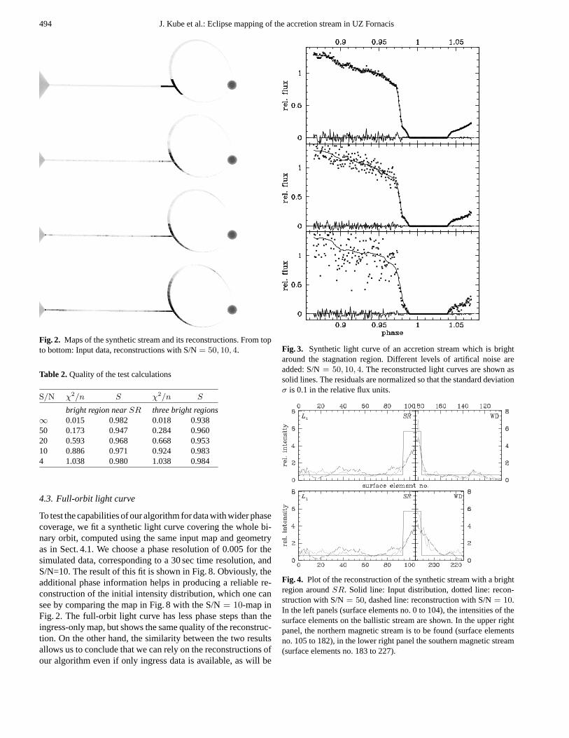
The light curves show small, but significant differences for thetwo orbits (Fig. 10). In orbit 1, the dip atΦ = 0.9 is slightlydeeper than in orbit 2. However, this very small feature has onlya marginal effect on the results. The dip is well known from X-Ray and EUV observations (Warren et al. 1995) and has beenobserved to move in phase betweenΦ = 0.88 and 0.92 ontimescales of months (Sirk & Howell 1998). The ingress of theaccretion stream into eclipse is much smoother in orbit 1 than inorbit 2, where an intermediate brightness level aroundΦ = 0.98with a flatter slope is seen. The Civ intensity maps resultingfrom our fits are shown in Fig. 11 for each observation intervalseparately. In Fig. 12, we show the relative intensity distribu-tions of 10 fit runs for each orbit, proving that our algorithmfinds the same result (except for noise) for each run. In Fig. 11,the resulting map from one arbitrary fit is shown.

The brightness maps for the two orbits show common fea-tures and differences. Common in both reconstructed maps arethe bright regions (1) on the ballistic stream, (2) on the dipole

stream above the orbital plane, and (3) on the dipole streambelow the orbital plane. In orbit 1, there is an additional brightregion on the northern dipole stream which appears as a mirrorimage of region 3. We denominate it 3b. The difference betweenboth maps is found in the presence/absence of region 3b, and inthe different sharpness of region 1, which is much brighter andmore peaked in orbit 1 than in orbit 2.

Remarkable is that we do not find a bright region at thecoupling regionSR, where one would expect dissipative heatingwhen the matter rams into the magnetic field and is decelerated.We will comment on this result in Sect. 6.2.

The sharp upper border of region 2 has to be discussedseparately: As one can see from the data, the flux of theC iv λ 1550 emission ceases completely in the phase intervalΦ ≈ 0.01 . . . 0.03. Hence, all parts of the accretion streamwhich are not eclipsed during this phase interval can not emitlight in C iv λ 1550. For the assumed geometry of UZ For, partsof the northern dipole stream remain visible throughout theeclipse. Thus, the sharp limitation of region 2 marks the borderbetween those surface elements which are always visible andthose which dissappear behind the secondary star. Uncertaintiesin the geometry could affect the location of the northern bound-ary of region 2, but should not change the general result, namelythat there is emissionabovethe orbital plane that accounts fora large part of the total stream emission in Civ λ 1550.

Region 3b has to be understood as an artifact: During orbit1, the observed flux level at maximum emission line eclipse(Φ = 0.01 . . . 0.03) does not drop to zero. Hence, our algorithmplaces intensity on the surface elements of the accretion stream

498 J. Kube et al.: Eclipse mapping of the accretion stream in UZ Fornacis

Fig. 12.Resulting intensity distributions of the accretion stream in UZ For. Left: Orbit 1, right: Orbit 2. The results of 10 individual fit runs areoverplotted in one graph to show the consistency of the fits. For an explanation of the plots see Fig. 4.

which are still visible at that phase. Apparently, the evolutionstrategy tends to place these residual emission not uniformlyon all the visible surface elements but on those closer to theWD, which leads to an intensity pattern that resembles the moreintense region on the southern side of the dipole stream.

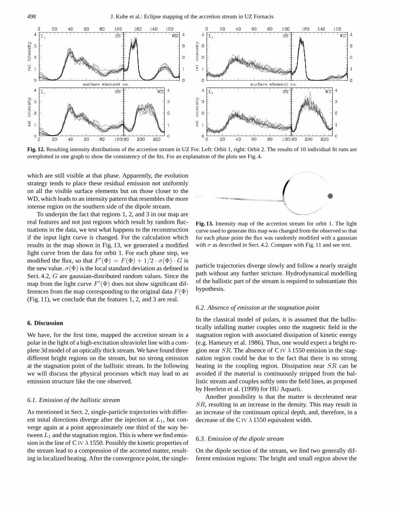
To underpin the fact that regions 1, 2, and 3 in our map arereal features and not just regions which result by random fluc-tuations in the data, we test what happens to the reconstructionif the input light curve is changed. For the calculation whichresults in the map shown in Fig. 13, we generated a modifiedlight curve from the data for orbit 1. For each phase step, wemodified the flux, so thatF ′(Φ) = F (Φ) + 1/2 · σ(Φ) · G isthe new value.σ(Φ) is the local standard deviation as defined inSect. 4.2,G are gaussian-distributed random values. Since themap from the light curveF ′(Φ) does not show significant dif-ferences from the map corresponding to the original dataF (Φ)(Fig. 11), we conclude that the features 1, 2, and 3 are real.

6. Discussion

We have, for the first time, mapped the accretion stream in apolar in the light of a high-excitation ultraviolet line with a com-plete 3d model of an optically thick stream. We have found threedifferent bright regions on the stream, but no strong emissionat the stagnation point of the ballistic stream. In the followingwe will discuss the physical processes which may lead to anemission structure like the one observed.

6.1. Emission of the ballistic stream

As mentioned in Sect. 2, single-particle trajectories with differ-ent inital directions diverge after the injection atL1, but con-verge again at a point approximately one third of the way be-tweenL1 and the stagnation region. This is where we find emis-sion in the line of Civ λ 1550. Possibly the kinetic properties ofthe stream lead to a compression of the accreted matter, result-ing in localized heating. After the convergence point, the single-

Fig. 13. Intensity map of the accretion stream for orbit 1. The lightcurve used to generate this map was changed from the observed so thatfor each phase point the flux was randomly modified with a gaussianwith σ as described in Sect. 4.2. Compare with Fig. 11 and see text.

particle trajectories diverge slowly and follow a nearly straightpath without any further stricture. Hydrodynamical modellingof the ballistic part of the stream is required to substantiate thishypothesis.

6.2. Absence of emission at the stagnation point

In the classical model of polars, it is assumed that the ballis-tically infalling matter couples onto the magnetic field in thestagnation region with associated dissipation of kinetic energy(e.g. Hameury et al. 1986). Thus, one would expect a bright re-gion nearSR. The absence of Civ λ 1550 emision in the stag-nation region could be due to the fact that there is no strongheating in the coupling region. Dissipation nearSR can beavoided if the material is continuously stripped from the bal-listic stream and couples softly onto the field lines, as proposedby Heerlein et al. (1999) for HU Aquarii.

Another possibility is that the matter is decelerated nearSR, resulting in an increase in the density. This may result inan increase of the continuum optical depth, and, therefore, in adecrease of the Civ λ 1550 equivalent width.

6.3. Emission of the dipole stream

On the dipole section of the stream, we find two generally dif-ferent emission regions: The bright and small region above the

J. Kube et al.: Eclipse mapping of the accretion stream in UZ Fornacis 499

α

αr

R

WD

1

2

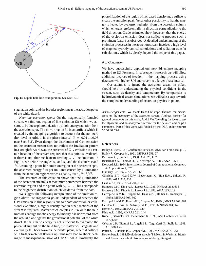
Fig. 14.Dipole field line configuration. See Sect. 6.3.

stagnation point and the broader regions near the accretion polesof the white dwarf.

Near the accretion spots:On the magnetically funneledstream, we find one region of line emission (3) which we as-sume to be due to photoionization by high-energy radiation fromthe accretion spot. The mirror region 3b is an artifact which iscreated by the mapping algorithm to account for the non-zeroflux level in orbit 1 in the phase intervalΦ = 0.01 . . . 0.03(see Sect. 5.3). Even though the distribution of Civ emissionon the accretion stream does not reflect the irradiation patternin a straightforward way, the presence of Civ emission at a cer-tain location of the stream requires that this point is irradiated,if there is no other mechanism creating Civ line emission. InFig. 14, we define the anglesα1 andα2 and the distancesr andR. Assuming a point-like emission region at the accretion spot,the absorbed energy flux per unit area caused by illuminationfrom the accretion regions varies ascos α1 sinα2R

3/2/r2.The structure of this equation shows that the illumination

of the accretion stream is at maximum somewhere between theaccretion region and the point withα1 = 0. This correspondsto the brightness distribution which we derive from the data.

We suggest the following interpretation of the emission re-gion above the stagnation point: Independent of whether theC iv emission in this region is due to photoionozation or colli-sional excitation, a higher density than in other sections of thestream is required. Matter which couples inSR onto the fieldlines has enough kinetic energy to initially rise northward fromthe orbital plane against the gravitational potential of the whitedwarf. If the kinetic energy is not sufficient to overcome thepotential summit on the field line, the matter will stagnate andeventually fall back towards the orbital plane, where it collideswith further material flowing up. This may lead to shock heat-ing with subsequent emission of Civ λ 1550. Alternatively, the

photoinization of the region of increased density may suffice tocreate the emission peak. Yet another possibility is that the mat-ter is heated by cyclotron radiation from the accretion columnwhich emerges preferentially in direction perpendicular to thefield direction. Crude estimates show, however, that the energyof the cyclotron emission does not suffice to produce such aprominent feature as observed. A detailed understanding of theemission processes in the accretion stream involves a high levelof magnetohydrodynamical simulations and radiation transfercalculations, which is, clearly, beyond the scope of this paper.

6.4. Conclusion

We have successfully applied our new 3d eclipse mappingmethod to UZ Fornacis. In subsequent research we will allowadditional degrees of freedom in the mapping process, usingdata sets with higher S/N and covering a larger phase interval.

Our attempts to image the accretion stream in polarsshould help in understanding the physical conditions in thestream, such as density and temperature. By comparison tohydrodynamical stream simulations, we will take a step towardsthe complete understanding of accretion physics in polars.

Acknowledgements.We thank Hans-Christoph Thomas for discus-sions on the geometry of the accretion stream, Andreas Fischer forgeneral comments on this work, Andre Van Teeseling for ideas to testthe algorithm and an anonymous referee for the detailed and helpfulcomments. Part of this work was funded by the DLR under contract50 OR 99 03 6.

References

Bailey J., 1995, ASP Conference Series 85, ASP, San Francisco, p. 10Bailey J., Cropper M., 1991, MNRAS 253, 27Berriman G., Smith P.S., 1988, ApJ 329, L97Beuermann K., Thomas H.-C., Schwope A., 1988, A&A 195, L15Dorward S.E., 1994, International Journal of Computational Geometry

& Applications 4, 325Flannery B.P., 1975, ApJ 201, 661Gansicke B.T., Hoard D.W., Beuermann K., Sion E.M., Szkody P.,

1998, A&A 338, 933Hakala P.J., 1995, A&A 296, 164Hameury J.M., King A.R., Lasota J.P., 1986, MNRAS 218, 695Hameury J.M., King A.R., Lasota J.P., 1988, A&A 195, L12Harrop-Allin M.K., Cropper M., Hakala P.J., Hellier C., Ramseyer T.,

1999a, MNRAS 308, 807Harrop-Allin M.K., Hakala P.J., Cropper M., 1999b, MNRAS 302, 362Heerlein C., Horne K., Schwope A.D., 1999, MNRAS 304, 145Horne K., 1985, MNRAS 213, 129King A.R., 1993, MNRAS 261, 144Kube J., Gansicke B.T., Beuermann K., 1999, ASP Conference Series

157, p. 99Osborne J.P., Giommi P., Angelini L., Tagliaferri G., Stella L., 1988,

ApJ 328, L45Potter S.B., Hakala P.J., Cropper M., 1998, MNRAS 297, 1261Rechenberg I., 1994, Evolutionsstrategie ’94. No. 1 in Werkstatt Bionik

und Evolutionstechnik, frommann-holzboog, Stuttgart

500 J. Kube et al.: Eclipse mapping of the accretion stream in UZ Fornacis

Rousseau T., Fischer A., Beuermann K., Woelk U., 1996, A&A 310,526

Schwope A., Beuermann K., Thomas H.-C., 1990, A&A 230, 120Schwope A., Mengel S., Beuermann K., 1997, A&A 320, 181Sirk M.M., Howell S.B., 1998, ApJ 506, 824Skilling J., Bryan R.K., 1984, MNRAS 211, 111

Stockman H.S., Schmidt G.D., 1996, ApJ 468, 883Vrielmann S., Schwope A.D., 1999, ASP Conference Series 157, p. 93Warner B., 1995, Cataclysmic Variable Stars. In: Cambridge astro-

physics series 28, Chapt. 6, Cambridge University Press, CambridgeWarren J.K., Sirk M.M., Vallerga J.V., 1995, ApJ 445, 909Wynn G.A., King A.R., 1995, MNRAS 275, 9