A&A manuscript no.(will be inserted by hand later)

Your thesaurus codes are:06 (02.01.2; 03.13.2; 08.02.1; 08.02.2; 08.09.2 UZ For; 08.14.2)

ASTRONOMYAND

ASTROPHYSICSDecember 22, 1999

Eclipse Mapping of the Accretion Stream in UZ Fornacis?

J. Kube, B. T. Gansicke, and K. Beuermann

Universitats-Sternwarte Gottingen, Geismar Landstraße 11, D-37083 Gottingen, Germany

Received 4 August 1999 / Accepted 20 December 1999

Abstract. We present a new method to map the surfacebrightness of the accretion streams in AM Herculis sys-tems from observed light curves. Extensive tests of thealgorithm show that it reliably reproduces the intensitydistribution of the stream for data with a signal-to-noiseratio >∼ 5. As a first application, we map the accretionstream emission of C iv λ 1550 in the polar UZ Fornacisusing HST FOS high state spectra. We find three mainemission regions along the accretion stream: (1) On theballistic part of the accretion stream, (2) on the magnet-ically funneled stream near the primary accretion spot,and (3) on the magnetically funneled stream at a positionabove the stagnation region.

Key words: Accretion – Methods: data analysis – bina-ries: close – binaries: eclipsing – Stars: individual: UZ For– cataclysmic variables

1. Introduction

Polars, as AM Hers are commonly named due to theirhighly polarized emission, consist of a late type main-sequence star (red dwarf, secondary star) and a highlymagnetized white dwarf (WD, primary star). The reddwarf, filling its Roche volume, injects matter throughthe L1 point into the Roche volume of the WD. Unlikein non-magnetic systems, this material does not form anaccretion disc, but couples onto the magnetic field oncethe magnetic pressure exceeds the ram pressure. From thisstagnation region (SR) on, the accretion stream follows amagnetic field line until it impacts onto the white dwarfsurface. For a review of polars, see Warner (1995).

Send offprint requests to: Jens Kube, jkube@uni-goettingen.de? The observational part of this work is based on observa-

tions made with the NASA/ESA Hubble Space Telescope, ob-tained from the data Archive at the Space Telescope ScienceInstitute, which is operated by the Association of Universi-ties for Research in Astronomy, Inc., under NASA contractNAS 5-26555. These observations are associated with proposalID 4013.

1L SR

Fig. 1. Overview of our 3d-Model of a polar. L1 marks theinner lagrangian point, SR the position of the stagnation orcoupling region.

In systems with an inclination i >∼ 70◦, the secondarystar gradually eclipses the accretion stream during the in-ferior conjunction. Using tomographical methods, it is – inprinciple – possible to reconstruct the surface brightnessdistribution on the accretion stream from time resolvedobservations. This method has been successfully applied toaccretion discs in non-magnetic CVs (“eclipse mapping”,Horne (1985)). We present tests and a first application ofa new eclipse mapping code, which allows the reconstruc-tion of the intensity distribution on the accretion streamin magnetic CVs.

Similar attempts to map accretion streams in polarshave been investigated by Hakala (1995) and Vrielmannand Schwope (1999) for HU Aquarii. An improved versionof Hakala’s (1995) method has been presented by Harrop-Allin et al. (1999b) with application to real data for thesystem HU Aquarii (Harrop-Allin et al., 1999a). A draw-back of all these approaches is that they only consider theeclipse of the accretion stream by the secondary star. In re-ality, the geometry may be more complicated: the far sideof the magnetically coupled stream may eclipse stream el-ements close to the WD, as well as the hot accretion spoton the WD itself. The latter effect is commonly observedas a dip in the soft X-ray light curves prior to the eclipse(e.g. Sirk and Howell, 1998). The stream-stream eclipsemay be detected in data which are dominated by emissionfrom the accretion stream, e.g. in the light curves of high-excitation emission lines where the secondary contributesonly little to the line flux.

2 J. Kube et al.: Eclipse Mapping of the Accretion Stream in UZ Fornacis

Here, we describe a new accretion stream eclipse map-ping method, using a 3d code which can handle the fullcomplexity of the geometry together with an evolutionstrategy as fit algorithm. We present extensive tests ofthe method and map as a first application to real datathe accretion stream in UZ For emission of C iv λ 1550.

2. The 3d Cataclysmic Variable Model

Our computer code CVMOD generates N small surfaceelements (convex quadrangles, some of which are degen-erated to triangles), which represent the surfaces of theindividual components of the CV (WD, secondary, accre-tion stream) in three-dimensional space (Fig. 1). Usingsimple rotation algorithms, the position of each surfaceelement i = 1 . . .N can be computed for a given orbitalphase Φ.

The white dwarf is modelled as an approximatedsphere, using surface elements of nearly constant area(Gansicke et al., 1998). The secondary star is assumedto fill its Roche volume. Here, the surface elements arechoosen in such a way that their boundaries align withlongitude and latitude circles of the Roche surface, takingthe L1-point as the origin.

We generate the surface of the accretion stream in twoparts, (a) the ballistic part from L1 to SR, and (b) thedipole-part from SR to the surface of the white dwarf.

(a) For the ballistic part of the stream, we use single-particle trajectories. The equations of motion in the coro-tating frame are given by

x = +µx− x1

r31

− (1− µ)x− x2

r32

+ 2y + x (1)

y = −µy

r31

− (1− µ)y

r32

− 2x + y (2)

z = −µz

r31

− (1− µ)z

r32

(3)

Equation (3) has been added to Flannery’s (1975) set oftwo-dimensional equations. µ = (M1+M2)/M1 is the massfraction of the white dwarf, r1 and r2 are the distancesfrom the point (x, y, z) to the white dwarf and the sec-ondary, respectively, in units of the orbital separation a.The coordinate origin is at the centre of gravity, the x-axis is along the lines connecting the centres of the stars,the system rotates with the angular frequency ω aroundto the z-axis. The velocity vvv = (x, y, z) is given in units ofaω, v0v0v0 = (x0, y0, z0) is the initial velocity in the L1 point.

If z0 = 0, the trajectories resulting from the numer-ical integration of eq. (1) – (3) are restricted to the or-bital plane. However, calculating single-particle trajecto-ries with different initial velocity directions (allowing alsoz0 6= 0) shows that there is a region approximately onethird of the way downstream from L1 to SR where all tra-jectories pass within very small separations, correspondingto a striction of the accretion stream.

We define a 3d version of the stream as a tubewith a circular cross section with radius rTube = 5 ×108 cm centred on the single-particle trajectory for x =10 kms−1, y = z = 0.

(b) When the matter reaches SR, we switch from aballistic single-particle trajectory to a magnetically forceddipole geometry. The central trajectory is generated us-ing the dipole formula r = r0r0r0 sin2 α, where α is the anglebetween the dipole axis and the position of the particle(r, ϕ, α). This can be interpreted as the magnetic fieldline F passing through the stagnation point SR and thehot spots on the WD. Knowing F , we assume a circularcross section with the radius rSR = rTube = 5 × 108 cmfor the region where the dipole intersects the ballisticstream. This cross section is subject to transformation asα changes. Thus, the cross section of the stream is nolonger constant in space but bounded everywhere by thesame magnetic field lines.

Our accretion stream model involves several assump-tions: (1) The cross section of the stream itself is to someextent arbitrary because we consider it to be – for ourcurrent data, see below – essentially a line source. (2) Theneglect of the magnetic drag (King, 1993; Wynn and King,1995) on the ballistic part of the stream and the neglect ofdeformation of the dipole field cause the model stream todeviate in space from the true stream trajectory. While,in fact, the location of SR may fluctuate with accretionrate (as does the location of the Earth’s magnetopause),the evidence for a sharp soft X-ray absorption dip causedby the stream suggest that SR does not wander abouton time scales short compared to the orbital period. (3)The abrupt switch-over from the ballistic to the dipolepart of the stream may not describe the physics of SRcorrectly. This discrepancy, however, does not seriouslyaffect our results, because the eclipse tomography is sen-sitive primarily to displacements in the times of ingressand egress of SR which are constrained by the absorptiondip in the UV continuum (and, in principle, in soft X-rays). The ≈ 5 sec time bins of our observed light curvescorrespond to ≈ 108 cm in space at SR. Hence, our codeis insensitive to structure on a smaller scale. In fact, thesmallest resolved structures are much larger because ofthe noise level of our data. While our approach clearly in-volves several approximations, it is tailored to the desiredaim of mapping the accretion stream from the informationobtained from an emission line light curve.

In our current code, we restrict the possible bright-ness distribution so that for each stream segment, whichconsists of 16 surface elements forming a section of thetube-like stream, the intensity is the same, i.e. there isno intensity variation around the stream. For the currentdata, this is no serious drawback, since we only use obser-vations covering a small phase interval around the eclipse.Our results refer, therefore, to the stream brightness asseen from the secondary. From the present observations wecan not infer how the fraction of the stream illuminated by

J. Kube et al.: Eclipse Mapping of the Accretion Stream in UZ Fornacis 3

the X-ray/UV spot on the WD looks like. The required ex-tension of our computer code, allowing for brightness vari-ation around the stream, is straightforward. The presentversion of the code is, however, adapted to the data setconsidered here.

3. Light curve fitting

The basic idea of our eclipse mapping algorithm is toreconstruct the intensity distribution on the accretionstream by comparing and fitting a synthetic light curveto an observed one. The comparison between these lightcurves is done with a χ2-minimization, which is modifiedby means of a maximum entropy method. Sections 3.1describes the light curve generation, 3.2 the maximum en-tropy method, and 3.3 the actual fitting algorithm.

3.1. Light curve generation

In order to generate a light curve from the 3d model, it isneccessary to know which surface elements i are visible ata given phase Φ. We designate the set of visible surfacesV (Φ).

In general, each of the three components (WD, sec-ondary, accretion stream) may eclipse (parts of) the othertwo, and the accretion stream may partially eclipse it-self. This is a typical hidden surface problem. However, incontrast to the widespread computer graphics algorithmswhich work in the image space of the selected output de-vice (e.g. a screen or a printer), and which provide theinformation ‘pixel j shows surface i’, we need to work inthe object space, answering the question ‘is surface i vis-ible at phase Φ?’. For a recent review on object spacealgorithms see Dorward (1994). Unfortunately, there is noreadily available algorithm which fits our needs, thus weuse a self-designed 3d object-space hidden-surface algo-rithm. Let N be the number of surface elements of our 3dmodel. According to Dorward (1994), the time T neededto perform an object space visibility analysis goes likeT ∝ N log N . . . N2. Our algorithm performs its task inT ∝ N1.5...1.8, with the faster results during the eclipseof the system. It is obviously necessary to optimize thenumber of surface elements in order to minimize the com-putation time without getting too coarse a 3d grid.

Once V (Φ) has been determined, the angles betweenthe surface normals of i ∈ V (Φ) and the line of sight,and the projected areas Ai,Φ of i ∈ V (Φ) are computed.Designating the intensity of the surface element i at thewavelength λ with Ii,λ, the observed flux Fλ(Φ) is

Fλ(Φ) =∑

i∈V (Φ)

Ii,λAi(Φ) (4)

Here, two important assumptions are made: (a) the emis-sion from all surface elements is optically thick, and (b)the emission is isotropic, i.e. there is no limb darkeningin addition to the foreshortening of the projected area of

the surface elements. The computation of a synthetic lightcurve is straightforward. It suffices to compute Fλ(Φ) forthe desired set of orbital phases.

While the above mentioned algorithm can producelight curves for all three components, the WD, the sec-ondary, and the accretion stream, we constrain in the fol-lowing the computations of light curves to emission fromthe accretion stream only. Therefore, we treat the whitedwarf and the secondary star as dark opaque objects,screening the accretion stream.

3.2. Constraining the problem: MEM

In the eclipse mapping analysis, the number of free pa-rameters, i.e. the intensity of the N surface elements, istypically much larger than the number of observed datapoints. Therefore, one has to reduce the degrees of freedomin the fit algorithm in a sensible way. An approach whichhas proved successful for accretion discs is the maximumentropy method MEM (Horne, 1985). The basic idea is todefine an image entropy S which has to be maximized,while the deviation between synthetic and observed lightcurve, usually measured by χ2/n, is minimized (n is thenumber of phase steps or data points). Let Di be

Di =

N∑j=1

Ij exp(− (rrri − rrrj)2

2∆2

)N∑

j=1

exp(− (rrri − rrrj)2

2∆2

) (5)

the default image for the surface element i. Then the en-tropy is given by

S =

N∑i=1

Ii

(ln

Ii

Di− 1

)N∑

i=1

Ii

(6)

In Eq. (5), rrri and rrrj are the positions of the surface el-ements i and j. ∆ determines the range of the MEM inthat the default image (5) is a convolution of the actualimage with a Gaussian with the σ-width of ∆. Hence, theentropy measures the deviation of the actual image fromthe default image. An ideal entropic image (with no con-trast at all) has S = 1. We use ∆ = 1×109 cm ≈ 0.02a forour test calculations and for the application to UZ For.

The quality of a intensity map is given as

Q = χ2/n− λS, (7)

where λ is chosen in the order of 1. Aim of the fit algorithmis to minimize Q.

3.3. The fitting algorithm: Evolution strategy

Our model involves approximately 250 parameters, whichare the intensities of the surface elements. This large num-ber is not the number of the degrees of freedom, which is

4 J. Kube et al.: Eclipse Mapping of the Accretion Stream in UZ Fornacis

Table 1. System geometry of the imaginary system IM Sys

mass ratio Q = M1/M2 = 4total mass M = M1 + M2 = 0.9M�orbital period P = 100 mininclination i = 88◦

dipole tilt β = 20◦

dipole azimuth Ψ = 35◦

angle to SR ΨS = 35◦

difficult to define in a MEM-strategy. A suitable methodto find a parameter optimum with a least χ2 and a max-imum entropy value is a simplified imitiation of biologi-cal evolution, commonly referred to as ‘evolution strategy’(Rechenberg, 1994). The intensity information of the i sur-face elements is stored in the intensity vector III. Initially,we choose Ii = 1 for all i.

¿From this parent intensity map, a number of off-springs are created with Ii randomly changed by a smallamount, the so-called mutation. For all offsprings, thequality Q is calculated. The best offspring is selected to bethe parent of the next generation. An important featureof the evolution strategy is that the amount of mutationitself is also being evolved just as if it were part of theparameter vector. We use the C-program library evoC de-veloped by K. Trint and U. Utecht from the TechnischeUniversitat Berlin, which handles all the important steps(offspring generation, selection, stepwidth control).

In contrast to the classical maximum entropy optimi-sation (Skilling and Bryan, 1984), the evolution strategydoes not offer a quality parameter that indicates how closethe best-fit solution is to the global optimum. In order totest the stability of our method, we run the fit severaltimes starting from randomly distributed maps. All runsconverge to very similar intensity distributions III (see alsoFigs. 10 and 12). This type of test is common in evolutionstrategy or genetic algorithms (e.g. Hakala 1995). Eventhough this approach is not a statistically ‘clean’ test, itleaves us to conclude that we find the global optimum.

Fastest convergence is achieved with 40 to 100 off-springs in each generation. Finding a good fit (χ2/n)takes only on tenth to one fifth of the total computationtime, the remaining iterations are needed to improve thesmoothness of the intensity map, i.e. to maximize S. Ahybrid code using a classical optimization algorithm, e.g.Powell’s method, may speed up the regularization (Potteret al., 1998).

4. Tests

To test the quality and the limits of our method, we pro-duce synthetical test light curves with different noise levels(S/N = ∞, 50, 20, 10, 4). We then try to reproduce our ini-tial intensity distribution on the stream from the syntheticdata. Two tests with different intensity distributions are

performed. For both tests, the geometry of the imaginarysystem IM Sys is chosen as shown in Table 1. The phasecoverage is Φ = 0.865 . . .1.070 with 308 equidistant steps,which is identical to the real HST data of UZ For whichwe use below for a first application.

Additionally, we test our algorithm with a full-orbitlight curve with S/N = 10 to demonstrate its capabilitiesif more than just the ingress information for each streamsection is available.

4.1. One bright region near SR

In the first test, we set the stream brightness to 1 on thewhole stream except for a small region near the stagna-tion point SR, where the intensity is set to 10. For thisintensity distribution, we show the theoretical light curvein Fig. 3. One clearly sees the fast ingress of the smallbright region at phase Φ = 0.975, whereas the egress oc-curs beyond Φ = 1.07 and is not covered as in the realdata of UZ For.

The initial intensity map and the reconstructed mapwith the different noise levels are shown in Figs. 2 and4. The reconstruction of one bright region near the stag-nation point is achieved with no artifacts, not too muchsmearing and little noise for S/N ≥ 10. Even with S/N =4, a reasonable reconstruction can be obtained, but withartifacts: The ballistic stream appears bright near the L1-point, and an additional bright region appears on thedipole stream near the northern accretion pole.

4.2. Three bright regions on the ballistic stream

In the second test we assume a rather unphysical intensitydistribution with the aim to test the spatial resolution ofour mapping method: The ballistic part of the accretionstream between L1 and SR is divided into 5 sections ofequal length. Alternately, the intensity on these sections isset equal to 10 and to 1, producing a ‘zebra’-like pattern.The intensity on the magnetically funneled stream is setto I = 1. The synthetic light curve for this intensity distri-bution differs strongly from that in out first test (Fig. 6).Instead of one sharp step in the light curve, there are now– as expected – three steps during the ingress and threeduring the egress (also not visible in the selected phaseinterval).

In Figs. 5 and 7 we show the input and the result-ing maps for the ‘zebra’-test. As long as S/N ≥ 10, ouralgorithm achieves, as in the first test, a good reconstruc-tion of the input map. The bright regions next to SRappear darker than in the original map, since the inten-sity from that region is spread over the last part of theballistic stream and the neighbouring parts of the dipolestream, which dissapear behind the limb of the secondarystar nearly simultaneously during ingress.

Comparing the two tests for S/N = 4, we find that it isstill possible to distinguish between the two different ini-

J. Kube et al.: Eclipse Mapping of the Accretion Stream in UZ Fornacis 5

Fig. 2. Maps of the synthetic stream and its reconstructions.From top to bottom: Input data, reconstructions with S/N =50, 10, 4.

Fig. 3. Synthetic light curve of an accretion stream which isbright around the stagnation region. Different levels of artifi-cal noise are added: S/N = 50, 10, 4. The reconstructed lightcurves are shown as solid lines. The residuals are normalized sothat the standard deviation σ is 0.1 in the relative flux units.

Fig. 4. Plot of the reconstruction of the syn-thetic stream with a bright region around SR.Solid line: Input distribution, dotted line: re-construction with S/N = 50, dashed line: re-construction with S/N = 10. In the left panels(surface elements no. 0 to 104), the intensitiesof the surface elements on the ballistic streamare shown. In the upper right panel, the north-ern magnetic stream is to be found (surface el-ements no. 105 to 182), in the lower right panelthe southern magnetic stream (surface elementsno. 183 to 227).

6 J. Kube et al.: Eclipse Mapping of the Accretion Stream in UZ Fornacis

Fig. 5. Maps of the synthetic stream and its reconstructions.From top to bottom: Input data, reconstructions with S/N =50, 10, 4.

Fig. 6. Synthetic light curve of an accretion stream with threebright parts on the ballistic stream. Different levels of artifi-cal noise are added: S/N = 50, 10, 4. The reconstructed lightcurves are shown as solid lines. The residuals are normalizedso that the standard deviation σ is at 0.1 in the relative flux.

Fig. 7. Plot of the reconstruction of the syn-thetic stream with three bright regions on theballistic stream. Solid line: Input distribution,dotted line: reconstruction with S/N = 50,dashed line: reconstruction with S/N = 10.For an explanation of the plot see Fig. 4

J. Kube et al.: Eclipse Mapping of the Accretion Stream in UZ Fornacis 7

Table 2. Quality and number of iterations for the test calcu-lations.

S/N χ2/n S χ2/n S

bright region near SR three bright regions∞ 0.015 0.982 0.018 0.93850 0.173 0.947 0.284 0.96020 0.593 0.968 0.668 0.95310 0.886 0.971 0.924 0.9834 1.038 0.980 1.038 0.984

tial intensity distributions (one bright region and ‘zebra’)even with such a noisy signal.

In Table 2, we list the quality parameters of the fits.The increase of χ2/n from ≈ 0 to ≈ 1 with the decreaseof S/N shows once more how well the fit algorithm works:For the light curve with no noise, the ideal light curve has– by definition – χ2 = 0. As soon as noise is added, eventhe input light curve has a χ2/n ≈ 1, which follows alsofrom the definition of χ2 if σ is the real standard devia-tion of the data set. For the calculation of χ2, one needsa sensibly chosen standard deviation σ. Since the lightcurves of polars show pronounced flickering, we calculatean approximate σ for our noisy data sets (synthetic andmeasured) by comparing the data with a running meanover 10 phase steps. The running mean has, thus, a re-duced χ2 of 1. Since the best fit to artificial data with lowsynthetic noise levels does better than the running mean,we obtain χ2/n < 1 for these light curves.

The entropy S of the images is always close to 1. Anideal entropic image would have S = 1, the actual valuesof S = 0.94 . . .0.98 come very close to that. One wouldnot expect S = 1, since that would imply that there is novariation in the image, i.e., all surface elements have thesame brightness. The trend to higher S with lower noiseis a result of the weighting of S with respect to χ2/n inthe one-dimensional quality parameter Q (Eq. 7). For thetest calculations, we have chosen λ = 1 constant for allnoise levels. This emphasizes the reduction of χ2 for lownoise levels and the smoothing for high noise levels.

Our tests show that we are able to detect structures inthe brightness distribution on the accretion stream with asize of ≈ 1 . . . 2R1 from data with phase coverage, phaseresolution and noise level similar to that of the HST dataset for UZ For (see section 5.2).

4.3. Full-orbit light curve

To test the capabilities of our algorithm for data withwider phase coverage, we fit a synthetic light curve cover-ing the whole binary orbit, computed using the same inputmap and geometry as in Sect. 4.1. We choose a phase res-olution of 0.005 for the simulated data, corresponding to a30 sec time resolution, and S/N=10. The result of this fitis shown in Fig. 8. Obviously, the additional phase infor-

Fig. 8. Top: Full-orbit reconstruction of the ‘point’-brightnessdistribution. Compare to Fig. 2, top. Bottom: Full-orbit syn-thetic light curve and best-fit light curve. For clarity, two fullorbits are shown.

mation helps in producing a reliable reconstruction of theinitial intensity distribution, which one can see by com-paring the map in Fig. 8 with the S/N = 10-map in Fig.2. The full-orbit light-curve has less phase steps than theingress-only-map, but shows the same quality of the re-construction. On the other hand, the similarity betweenthe two results allows us to conclude that we can rely onthe reconstructions of our algorithm even if only ingressdata is available, as will be the case for the HST archivedata of UZ For which we use in the following.

The synthetic light curve over the full orbit shows var-ious eclipse and projection features, which are describedin detail by Kube et al. (1999).

5. Application: UZ For

5.1. System Geometry of UZ For

UZ For has been identified as a polar in 1988 (Berrimanand Smith, 1988; Beuermann et al., 1988; Osborne et al.,1988). Cyclotron radiation from a region with B = 53 MGhas been reported by Schwope et al. (1990) and Rousseauet al. (1996). The first mass estimates for the WD wererather high, M1 = 1.09 ± 0.01M� and M1 > 0.93M�(Hameury et al., 1988; Beuermann et al., 1988), but Baileyand Cropper (1991) and Schwope et al. (1997) derived sig-nificantly smaller masses, 0.61M� < M1 < 0.79M� andM1 = 0.75M�, respectively. We use reliable system pa-

8 J. Kube et al.: Eclipse Mapping of the Accretion Stream in UZ Fornacis

Table 3. System geometry of UZ Fornacis

mass ratio Q = M1/M2 = 5total mass M = M1 + M2 = 0.85M�orbital period P = 126.526 229 minorbital separation a = 5.49 × 1010 cminclination i = 81◦

radius of WD R1 = 7.53 × 108 cm

dipole tilt β = 12◦

dipole azimuth Ψ = 5◦

azimuth of stagnation region ΨS = 34◦

‘radius’ of ballistic stream rS = 5× 108 cm

rameters from Bailey and Cropper (1991), q = M1/M2 =5, M = M1 +M2 = 0.85 M�, i = 81◦, P = 126.5 min. Theoptical light curve in Bailey (1995) shows two eclipse stepswhich are interpreted as the signature of hot spots nearboth magnetic poles of the WD, consecutively dissapear-ing behind the limb of the secondary star. From that lightcurve we measure the timing of the eclipse events with anaccuracy of ∆Φ = 5 · 10−4. The ingress of the spot onthe lower hemisphere occurs at Φ = 0.9685, its egress atΦ = 1.0310. For the spot on the upper hemisphere, ingressis at Φ = 0.9725 and egress at Φ = 1.0260.

To describe the spatial position of the dipole fieldline along which the matter is accreted, three angles areneeded: The colatitude or tilt of the dipole axis β, thelongitude of the dipole axis Ψ, and the longitude of thestagnation region ΨS. Here, longitude is the angle betweenthe secondary star and the respective point as seen fromthe centre of the white dwarf. With our choice of β, Ψ,and ΨS , we can reproduce the ingress and egress of thetwo hot spots as well as the dip at phase Φ = 0.9. A sum-mary of the main system parameters used in this analysisis given in Table 3.

Having the correct geometry of the accretion streamis crucial for generating the correct reconstruction of theemission regions. As we have shown in (Kube et al., 1999)especially the geometry of the dipole stream is sensitiveto changes in Ψ, ΨS , and β. For UZ For, the geometryof the dipole stream is relatively well constrained fromthe observed ingress and egress of both hot spots on thewhite dwarf (Bailey, 1995). Fitting the UZ For light curvessystem geometries that differ within the estimated errorrange of less than five degrees does, however, not signifi-cantly affect our results. This situation is different if theerrors in the geometry parameters are larger than only afew degrees.

5.2. Observational Data

UZ For was observed with HST on June 11, 1992. A de-tailed description of the data is given by Stockman and

Schmidt (1996). We summarize here only the relevantpoints.

Fast FOS/G160L spectroscopy with a time resolutionof 1.6914 s was obtained, covering two entire eclipses inthe phase interval Φ = 0.87 . . .1.07. The two eclipseswere observed starting at 05:05:33 UTC (‘orbit 1’) and11:25:39 UTC (‘orbit 2’). The spectra cover the range1180 . . .2500 A with a FWHM resolution of ≈ 7 A. Themid-exposure times of the individual spectra were con-verted into binary orbital phases using the ephemeris ofWarren et al. (1995). The average trailed spectrum isshown in Fig. 9.

In order to obtain a light curve dominated by the ac-cretion stream, we extracted the continuum subtractedC iv λ 1550 emission from the trailed spectrum. The re-sulting light curves are shown in Fig. 10 for both orbitsseparately. To reduce the noise to a bearable amount, thelight curves were rebinned to 5.07 s resulting in a phaseresolution of ∆Φ = 6.7× 10−4.

We note that the C iv light curve may be contami-nated by emission from the heated side of the secondarystar. HST/GHRS observations of AM Her, which resolvethe broad component originating in the stream and thenarrow component originating on the secondary, show thatthe contribution of the narrow component to the total fluxof C iv is unlikely to be larger than 10 . . . 15% (Gansickeet al., 1998). Furthermore, during the phase interval cov-ered in the HST observations of UZ For, the irradiatedhemisphere of the secondary is (almost) completely self-eclipsed, so that its C iv emission is minimized.

5.3. Results

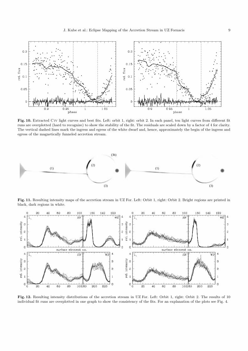
The light curves show small, but significant differences forthe two orbits (Fig. 10). In orbit 1, the dip at Φ = 0.9 isslightly deeper than in orbit 2. However, this very smallfeature has only a marginal effect on the results. The dipis well known from X-Ray and EUV observations (War-ren et al., 1995) and has been observed to move in phasebetween Φ = 0.88 and 0.92 on timescales of months (Sirkand Howell, 1998). The ingress of the accretion streaminto eclipse is much smoother in orbit 1 than in orbit 2,where an intermediate brightness level around Φ = 0.98with a flatter slope is seen. The C iv intensity maps result-ing from our fits are shown in Fig. 11 for each observationinterval separately. In Fig. 12, we show the relative inten-sity distributions of 10 fit runs for each orbit, proving thatour algorithm finds the same result (except for noise) foreach run. In Fig. 11, the resulting map from one arbitraryfit is shown.

The brightness maps for the two orbits show commonfeatures and differences. Common in both reconstructedmaps are the bright regions (1) on the ballistic stream,(2) on the dipole stream above the orbital plane, and (3)on the dipole stream below the orbital plane. In orbit 1,there is an additional bright region on the northern dipole

J. Kube et al.: Eclipse Mapping of the Accretion Stream in UZ Fornacis 9

Fig. 10. Extracted C iv light curves and best fits. Left: orbit 1, right: orbit 2. In each panel, ten light curves from different fitruns are overplotted (hard to recognize) to show the stability of the fit. The residuals are scaled down by a factor of 4 for clarity.The vertical dashed lines mark the ingress and egress of the white dwarf and, hence, approximately the begin of the ingress andegress of the magnetically funneled accretion stream.

(1)(2)

(3)

(3b)

(1)(2)

(3)

Fig. 11. Resulting intensity maps of the accretion stream in UZ For. Left: Orbit 1, right: Orbit 2. Bright regions are printed inblack, dark regions in white.

Fig. 12. Resulting intensity distributions of the accretion stream in UZ For. Left: Orbit 1, right: Orbit 2. The results of 10individual fit runs are overplotted in one graph to show the consistency of the fits. For an explanation of the plots see Fig. 4.

10 J. Kube et al.: Eclipse Mapping of the Accretion Stream in UZ Fornacis

Fig. 9. Trailed spectrum of UZ For, both observed orbits addedand rebinned. The figure clearly shows the abrupt ingress andegress of the continuum source and the more gradual eclipseof the emission line source. It also shows a faint dip in thecontinuum and in the lines at Φ = 0.90 which occurs when themagnetically funneled section of the accretion stream crossesthe line of sight to the white dwarf.

stream which appears as a mirror image of region 3. Wedenominate it 3b. The difference between both maps isfound in the presence/absence of region 3b, and in thedifferent sharpness of region 1, which is much brighterand more peaked in orbit 1 than in orbit 2.

Remarkable is that we do not find a bright region at thecoupling region SR, where one would expect dissipativeheating when the matter rams into the magnetic field andis decelerated. We will comment on this result in Sect. 6.2.

The sharp upper border of region 2 has to be discussedseparately: As one can see from the data, the flux of theC iv λ 1550 emission ceases completely in the phase in-terval Φ ≈ 0.01 . . .0.03. Hence, all parts of the accretionstream which are not eclipsed during this phase intervalcan not emit light in C iv λ 1550. For the assumed geome-try of UZ For, parts of the northern dipole stream remainvisible throughout the eclipse. Thus, the sharp limitationof region 2 marks the border between those surface ele-ments which are always visible and those which dissappearbehind the secondary star. Uncertainties in the geometrycould affect the location of the northern boundary of re-gion 2, but should not change the general result, namelythat there is emission above the orbital plane that accountsfor a large part of the total stream emission in C ivλ 1550.

Region 3b has to be understood as an artifact: Duringorbit 1, the observed flux level at maximum emission lineeclipse (Φ = 0.01 . . .0.03) does not drop to zero. Hence,

Fig. 13. Intensity map of the accretion stream for orbit 1. Thelight curve used to generate this map was changed from theobserved so that for each phase point the flux was randomlymodified with a gaussian with σ as described in Sect. 4.2. Com-pare with Fig. 11 and see text.

our algorithm places intensity on the surface elements ofthe accretion stream which are still visible at that phase.Apparently, the evolution strategy tends to place theseresidual emission not uniformly on all the visible surfaceelements but on those closer to the WD, which leads to anintensity pattern that resembles the more intense regionon the southern side of the dipole stream.

To underpin the fact that regions 1, 2, and 3 in ourmap are real features and not just regions which resultby random fluctuations in the data, we test what happensto the reconstruction if the input light curve is changend.For the calculation which results in the map shown in Fig.13, we generated a modified light curve from the data fororbit 1. For each phase step, we modified the flux, so thatF ′(Φ) = F (Φ) + 1/2 · σ(Φ) · G is the new value. σ(Φ) isthe local standard deviation as defined in Sect. 4.2, G aregaussian-distributed random values. Since the map fromthe light curve F ′(Φ) does not show significant differencesfrom the map corresponding to the original data F (Φ)(Fig. 11), we conclude that the features 1, 2, and 3 arereal.

6. Discussion

We have, for the first time, mapped the accretion streamin a polar in the light of a high-excitation ultraviolet linewith a complete 3d model of an optically thick stream. Wehave found three different bright regions on the stream,but no strong emission at the stagnation point of the bal-listic stream. In the following we will discuss the physicalprocesses which may lead to an emission structure like theone observed.

6.1. Emission of the ballistic stream

As mentioned in Sect. 2, single-particle trajectories withdifferent inital directions diverge after the injection at L1,but converge again at a point approximately one third ofthe way between L1 and the stagnation region. This iswhere we find emission in the line of C iv λ 1550. Possiblythe kinetic properties of the stream lead to a compressionof the accreted matter, resulting in localized heating. Af-

J. Kube et al.: Eclipse Mapping of the Accretion Stream in UZ Fornacis 11

ter the convergence point, the single-particle trajectoriesdiverge slowly and follow a nearly straight path withoutany further stricture. Hydrodynamical modelling of theballistic part of the stream is required to substantiate thishypothesis.

6.2. Absence of emission at the stagnation point

In the classical model of polars, it is assumed that the bal-listically infalling matter couples onto the magnetic field inthe stagnation region with associated dissipation of kineticenergy (e.g. Hameury et al., 1986). Thus, one would expecta bright region near SR. The absence of C ivλ 1550 emi-sion in the stagnation region could be due to the fact thatthere is no strong heating in the coupling region. Dissipa-tion near SR can be avoided if the material is continouslystripped from the ballistic stream and couples softly ontothe field lines, as proposed by Heerlein et al. (1999) forHU Aquarii.

Another possibility is that the matter is deceleratednear SR, resulting in an increase in the density. This mayresult in an increase of the continuum optical depth, and,therefore, in a decrease of the C ivλ 1550 equivalent width.

6.3. Emission of the dipole stream

On the dipole section of the stream, we find two generallydifferent emission regions: The bright and small regionabove the stagnation point and the broader regions nearthe accretion poles of the white dwarf.

Near the accretion spots: On the magnetically funneledstream, we find one region of line emission (3) which weassume to be due to photoionization by high-energy radi-ation from the accretion spot. The mirror region 3b is anartifact which is created by the mapping algorithm to ac-count for the non-zero flux level in orbit 1 in the phaseinterval Φ = 0.01 . . . 0.03 (see Sect. 5.3). Even thoughthe distribution of C iv emission on the accretion streamdoes not reflect the irradiation pattern in a straigthfor-ward way, the presence of C iv emission at a certain loca-tion of the stream requires that this point is irradiated, ifthere is no other mechanism creating C iv line emission.In Fig. 14, we define the angles α1 and α2 and the dis-tances r and R. Assuming a point-like emission region atthe accretion spot, the absorbed energy flux per unit areacaused by illumiation from the accretion regions varies ascosα1 sin α2R

3/2/r2. The structure of this equation showsthat the illumination of the accretion stream is at max-imum somewhere between the accretion region and thepoint with α1 = 0. This corresponds to the brightnessdistribution which we derive from the data.

We suggest the following interpretation of the emissionregion above the stagnation point : Independent of whetherthe C iv emission in this region is due to photoionozationor collisional excitation, a higher density than in othersections of the stream is required. Matter which couples

α

αr

R

WD

1

2

Fig. 14. Dipole field line configuration. See Sect. 6.3.

in SR onto the field lines has enough kinetic energy toinitially rise northward from the orbital plane against thegravitational potential of the white dwarf. If the kineticenergy is not sufficient to overcome the potential summiton the field line, the matter will stagnate and eventuallyfall back towards the orbital plane, where it collides withfurther material flowing up. This may lead to shock heat-ing with subsequent emission of C iv λ 1550. Alternatively,the photoinization of the region of increased density maysuffice to create the emission peak. Yet another possibil-ity is that the matter is heated by cyclotron radiationfrom the accretion column which emerges preferentiallyin direction perpendicular to the field direction. Crude es-timates show, however, that the energy of the cyclotronemission does not suffice to produce such a prominent fea-ture as observed. A detailed understanding of the emissionprocesses in the accretion stream involves a high level ofmagnetohydrodynamical simulations and radiation trans-fer calculations, which is, clearly, beyond the scope of thispaper.

6.4. Conclusion

We have successfully applied our new 3d eclipse mappingmethod to UZ Fornacis. In subsequent research we willallow additional degrees of freedom in the mapping pro-cess, using data sets with higher S/N and covering a largerphase interval.

Our attempts to image the accretion stream in polarsshould help in understanding the physical conditions inthe stream, such as density and temperature. By compar-ison to hydrodynamical stream simulations, we will takea step towards the complete understanding of accretionphysics in polars.

Acknowledgements. We thank Hans-Christoph Thomas fordiscussions on the geometry of the accretion stream, Andreas

12 J. Kube et al.: Eclipse Mapping of the Accretion Stream in UZ Fornacis

Fischer for general comments on this work, Andre Van Teesel-ing for ideas to test the algorithm and an anonymous refereefor the detailed and helpful comments. Part of this work wasfunded by the DLR under contract 50 OR99 03 6.

References

Bailey, J., 1995, No. 85 in ASP Conference Series, pp 10–20, Astronomical Society of the Pacific, San Francisco

Bailey, J. and Cropper, M., 1991, MNRAS 253, 27Berriman, G. and Smith, P. S., 1988, ApJ 329, L97Beuermann, K., Thomas, H.-C., and Schwope, A., 1988,

A&A 195, L15Dorward, S. E., 1994, International Journal of Computa-

tional Geometry & Applications 4, 325Flannery, B. P., 1975, ApJ 201, 661Gansicke, B. T., Hoard, D. W., Beuermann, K., Sion,

E. M., and Szkody, P., 1998, A&A 338, 933Hakala, P. J., 1995, A&A 296, 164Hameury, J. M., King, A. R., and Lasota, J. P., 1986,

MNRAS 218, 695Hameury, J. M., King, A. R., and Lasota, J. P., 1988,

A&A 195, L12Harrop-Allin, M. K., Cropper, M., Hakala, P. J., Hellier,

C., and Ramseyer, T., 1999a, MNRAS 308, 807Harrop-Allin, M. K., Hakala, P. J., and Cropper, M.,

1999b, MNRAS 302, 362Heerlein, C., Horne, K., and Schwope, A. D., 1999, MN-

RAS 304, 145Horne, K., 1985, MNRAS 213, 129King, A. R., 1993, MNRAS 261, 144Kube, J., Gansicke, B. T., and Beuermann, K., 1999,

No. 157 in ASP Conference Series, pp 99–103Osborne, J. P., Giommi, P., Angelini, L., Tagliaferri, G.,

and Stella, L., 1988, ApJ 328, L45Potter, S. B., Hakala, P. J., and Cropper, M., 1998, MN-

RAS 297, 1261Rechenberg, I., 1994, Evolutionsstrategie ’94, No. 1 in

Werkstatt Bionik und Evolutionstechnik, frommann-holzboog, Stuttgart

Rousseau, T., Fischer, A., Beuermann, K., and Woelk, U.,1996, A&A 310, 526

Schwope, A., Beuermann, K., and Thomas, H.-C., 1990,A&A 230, 120

Schwope, A., Mengel, S., and Beuermann, K., 1997, A&A320, 181

Sirk, M. M. and Howell, S. B., 1998, ApJ 506, 824Skilling, J. and Bryan, R. K., 1984, MNRAS 211, 111Stockman, H. S. and Schmidt, G. D., 1996, ApJ 468, 883Vrielmann, S. and Schwope, A. D., 1999, No. 157 in ASP

Conference Series, pp. 93–98Warner, B., 1995, Cataclysmic Variable Stars, Chapt. 6,

No. 28 in Cambridge astrophysics series, CambridgeUniversity Press, Cambridge

Warren, J. K., Sirk, M. M., and Vallerga, J. V., 1995, ApJ445, 909

Wynn, G. A. and King, A. R., 1995, MNRAS 275, 9