Assignment 3 Solution

1. Solution for Q1:

From Y = a/X, we havedy

dx= − a

x2x =

a

y

and ∣∣∣∣∣dy

dx

∣∣∣∣∣ =

∣∣∣∣∣y2

a

∣∣∣∣∣ fY (y) =∑

i

1

|dy/dx|i fX(xi)

therefore,

when a > 0 fY (y) =a

y2fX

(a

y

)(1)

when a < 0 fY (y) = − a

y2fX

(a

y

)(2)

2. Solution for Q2:

Since Y = cX2,

dy

dx= 2cx and two roots at x1 =

√y

c, x2 = −

√y

c

Therefore,

fY (y) =∑

i

1

|dy/dx|i fX(xi) =1

2c√

yc

(fX(

√y

c) + fX(−

√y

c))

=fX(

√yc) + fX(−

√yc)

2√

cy(3)

while

fX(x) =1

2a(−a < x < a)

while implies 0 < y < ca2. Therefore,

fY (y) =1/2a + 1/2a

2√

cy=

1

2a√

cy0 < y < ca2

3. Solution for Q3:

fX(x) =1√2πσ

e−x2

2σ2 and Y = g(X) = 5X2

E[Y ] =∫ ∞

−∞f(x)fX(x) dx =

∫ ∞

−∞5x2· 1√

2πσe−

x2

2σ2 dx = 5∫ ∞

−∞x2· 1√

2πσe−

x2

2σ2 dx = 5σ2 = 45

The last integral is the variance of zero mean Gaussian RV, we can obtain the result of the

integral directly without integration.

1

4. Solution for Q4:

(a)

P (X = −1) = P (ξ = −1) =1

5P (Y = 1) = P (ξ = −1) + P (ξ = 1) =

2

5while

P (X = −1, Y = 1) = P (ξ = −1) =1

5therefore,

P (X = −1) P (Y = 1) =1

5· 2

5=

2

256= P (X = −1, Y = 1)

hence, X and Y are dependent RVs.

(b)

E[X] =∑

xiP (xi) =5∑

i=1

ξiP (ξi) =1

5(−1− 1/2 + 0 + 1/2 + 1) = 0

E[Y ] =∑

yiP (yi) =5∑

i=1

ξ2i P (ξi) =

1

5(1 + 1/4 + 0 + 1/4 + 1) = 1/2

E[XY ] =∑

xyP (x, y) =5∑

i=1

ξ3P (ξ) =1

5(−1− 1/8 + 0 + 1/8 + 1) = 0

Since E[XY ] = E[X] · E[Y ], X and Y are uncorrelated RVs.

5. Solution for Q5:

Since,

Xn = Zn − aZn−1 |a| < 1

E[Zn] = 0 E[ZnZj] = 0 E[Z2n] = σ2

We have,

Rn(k) = E[XnXn−k] = E[(Zn − aZn−1)(Zn−k − aZn−k−1)]

= E[ZnZn−k − aZnZn−k−1 − aZn−1Zn−k + a2Zn−1Zn−k−1] (4)

Rn(0) = E[Z2n − 2aZn−1Zn + a2Z2

n−1 = (1 + a2)σ2

Rn(−1) = Rn(1) = E[ZnZn−1 − aZnZn−2 − aZ2n−1 + a2Zn−1Zn−2 = −aσ2

When k > 1, the expectation of each term in (4) equals zero. Therefore,

Rn(k) =

(1 + a2)σ2 k = 0

−aσ2 k = ±1

0 o.w.

2

6. Solution for Q6:

To find the constant c, we apply∫∞−∞

∫∞−∞ f(x, y) dx dy = 1

∫ ∞

−∞

∫ ∞

−∞f(x, y) dx dy =

∫ 2

0

∫ 1

0cxydxdy =

c

2

∫ 2

0y dy = c

therefore, c = 1. To calculate P (A), we write

P [A] =∫ ∫

Af(x, y) dx dy

we use polar coordinates, using x = r cos θ and y = r sin θ, and dx dy = rdr dθ,

P [A] =∫ π/2

0

∫ 1

0r2 sin θ cos θ r dr dθ =

∫ 1

0r3 dr

∫ pi/2

0sin θ cos θ dθ = 1/8

7. Solution for Q7:

First, find the constant c,∫ ∞

−∞

∫ ∞

−∞f(x, y) dx dy =

∫ 2π

0

∫ 1

0c · rdr dθ = 1

c · 2π · 1/2r2|10 = 1

Therefore, c = 1/pi. The probability that the distance from the origin is less than x is∫ 2π

0

∫ x

01/π · rdr dθ = 2πcdot

1

π· 1

2r2|x0 = x2

8. Solution for Q8:

Proof:

P [X ≤ Y ] =∫ ∫

x≤yfX(x)fY (y) dxdy =

∫ ∞

−∞

∫ y

−∞fX(x)fY (y) dxdy

=∫ ∞

−∞fY (y)

∫ y

−∞fX(x) dx dy =

∫ ∞

−∞fY (y)FX(y)dy (5)

9. Solution for Q9:

Proof:

E[XY ] = E[X]E[Y ] = µXµY

E[X2] = µ2X + σ2

X and E[Y 2] = µ2Y + σ2

Y

therefore,

E[(XY )2] = E[X2] · E[Y 2] = (µ2X + σ2

X)(µ2Y + σ2

Y )

hence,

V ar(XY ) = E[(XY )2]−E2[XY ] = (µ2X + σ2

X)(µ2Y + σ2

Y )−µ2Xµ2

Y = σ2Xσ2

Y + µ2Y σ2

X + µ2Xσ2

Y .

3

10. Solution for Q10:

Let RV. U = X + Y and V = X − Y , then the joint moment generating function is

Φ(ω1, ω2) = E (eω1u + eω2v) = E(eω1X+ω1Y +ω2X−ω2Y

)

= E(e(ω1+ω2)X+(ω1−ω2)Y

)

since X and Y are independent Gaussian ∼ N(µ, σ2), therefore,

Φ(ω1, ω2) = E[e(ω1+ω2)X

]· E

[e(ω1−ω2)Y

]

= exp

[µ(ω1 + ω2) +

σ2(ω1 + ω2)2

2

]· exp

[µ(ω1 − ω2) +

σ2(ω1 − ω2)2

2

]

= exp

[2µω1 +

σ2 · 2ω21

2+

σ2 · 2ω22

2

]

= exp

[2µω1 +

(2σ2) · ω21

2

]· exp

[(2σ2) · ω2

2

2

]

= Φ(ω1) · Φ(ω2) (6)

where we have applied the fact that U ∼ N(2µ, 2σ2) and V ∼ N(0, 2σ2). From (6), we can

obtain the result that U and V are independent.

11. Solution for Q11:

(a)

ΦXi(ωi) = Φ(0, 0, · · · , 0, ωi, 0, · · · , 0)

with ωi in the ith place, and all others to be 0.

(b) If independent, then the joint CF is

E[ej

∑ωiXi

]= E

[ejω1X1 · ejω2X2 · · ·

]=

∏

i

E[ejωiXi

]=

∏

i

ΦXi(ωi) (7)

On the other hand, if the above is satisfied, then the joint CF is that of the sum of n

independent random variables, and the ith of which has the same distribution as Xi. As

the joint CF uniquely determines the joint distribution, the results follows.

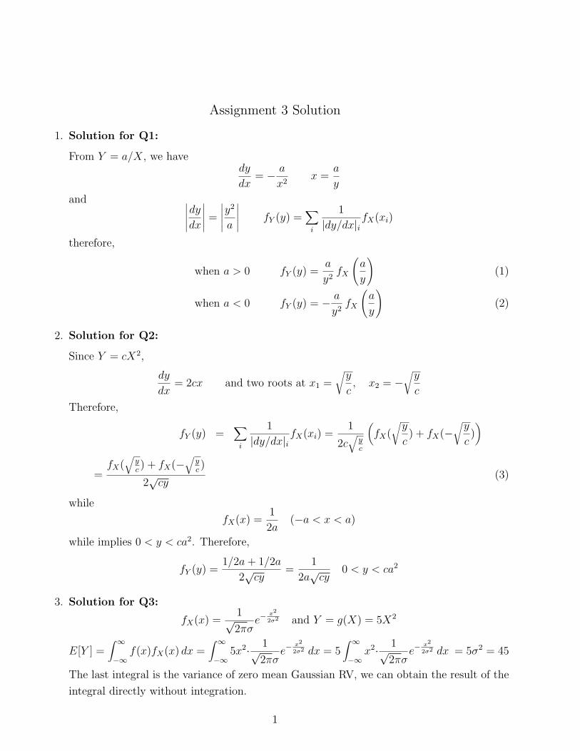
12. Solution for Q12:

It is easy to see that Y takes values only in the interval (9/11, 9/9) =(0.8182,1), as shown in

Fig.1. Therefore, the value of the distribution function, FY (v), is zero for v < 0.8182 and is

1 for v > 1. What happens between these two values can be inferred from the figure, where

a line of a value of v = 0.918 is shown, so that we see that for Y to fall below this value,

4

the value of Y has to be higher than 9/v, a point obtained by finding the inverse value of

the function 9/X. The resulting distribution function is obtained as follows:

FY (v) = P(

9

X≤ v

)= P

(X ≥ 9

v

)= (11− 9/v)/2 = 5.5− 4.5/v 0.8182 < v < 1

and

FY (v) = 0, v < 0.8182, or v > 1

The CDF of Y is shown in top figure in FIg.2. The density function of Y is obtained by

taking the derivative of the distribution function; for the values in the range (0.8182,1), it

has the expression:

fY (v) = 4.5/v2, 0.8182 < v < 1

and is zero elsewhere, as shown in the bottom figure in Fig.2. It is interesting to note that

even though X is uniformly distributed in the interval (9,11), the resulting current is not

uniformly distributed.

Figure 1: Y as a function of X, and a line showing one value of v (figure for Q12).

13. Solution for Q13:

(a) when v < −a, we obtain no value of Y , since Y takes values only between −a and +a,

which implies

FY (v) = P (Y ≤ v) = 0 v < −a

(b) Similarly, when v > +a, all values of Y will fall below the value of v, which means

FY (v) = P (Y ≤ v) = 1 v > +a

5

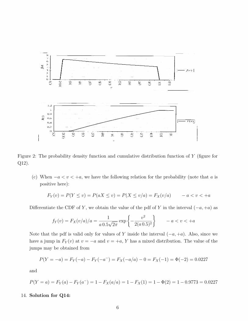
Figure 2: The probability density function and cumulative distribution function of Y (figure for

Q12).

(c) When −a < v < +a, we have the following relation for the probability (note that a is

positive here):

FY (v) = P (Y ≤ v) = P (aX ≤ v) = P (X ≤ v/a) = FX(v/a) − a < v < +a

Differentiate the CDF of Y , we obtain the value of the pdf of Y in the interval (−a, +a) as

fY (v) = FX(v/a)/a =1

a 0.5√

2πexp

{− v2

2(a 0.5)2

}− a < v < +a

Note that the pdf is valid only for values of Y inside the interval (−a, +a). Also, since we

have a jump in FY (v) at v = −a and v = +a, Y has a mixed distribution. The value of the

jumps may be obtained from

P (Y = −a) = FY (−a)− FY (−a−) = FX(−a/a)− 0 = FX(−1) = Φ(−2) = 0.0227

and

P (Y = a) = FY (a)−FY (a−) = 1−FX(a/a) = 1−FX(1) = 1−Φ(2) = 1− 0.9773 = 0.0227

14. Solution for Q14:

6

The pdf of Cauchy RV X with parameter α is give as

fX(x) =α/π

(x2 + α2)−∞ < x < ∞

The corresponding CF of X is given as

ΦX(ω) = e−α|ω|

Similarly, the CF of Y with parameter β is given as

ΦY (ω) = e−β|ω|

Since X and Y are independent, the CF of the sum RV Z = X + Y is

ΦZ(ω) = ΦX(ω) · ΦY (ω) = e−(α+β)|ω|

which is a CF of a Cauchy RV with parameter α + β, therefore, the cdf of Z is given as

fZ(z) =(α + β)/π

(z2 + (α + β)2)−∞ < z < ∞

7