Embed Size (px)
Citation preview

University of Texas at El PasoDigitalCommons@UTEP
Open Access Theses & Dissertations
2013-01-01
Assessment Of Abaqus Capabilities For CrackGrowth And Calculation Of Energy Release RateLuis Alonso HernandezUniversity of Texas at El Paso, [email protected]
Follow this and additional works at: https://digitalcommons.utep.edu/open_etdPart of the Mechanical Engineering Commons
This is brought to you for free and open access by DigitalCommons@UTEP. It has been accepted for inclusion in Open Access Theses & Dissertationsby an authorized administrator of DigitalCommons@UTEP. For more information, please contact [email protected].
Recommended CitationHernandez, Luis Alonso, "Assessment Of Abaqus Capabilities For Crack Growth And Calculation Of Energy Release Rate" (2013).Open Access Theses & Dissertations. 1840.https://digitalcommons.utep.edu/open_etd/1840

ASSESSMENT OF ABAQUS CAPABILITIES FOR CRACK GROWTH AND
CALCULATION OF ENERGY RELEASE RATE
LUIS A. HERNANDEZ
Department of Mechanical Engineering
APPROVED:
Jack F. Chessa, Ph.D., Chair
Yirong Lin, Ph.D.
Stephen W. Stafford, Ph.D.
Benjamin C. Flores, Ph.D. Dean of the Graduate School

Copyright ©
by
LUIS A. HERNANDEZ
2013

DEDICATION
I want to dedicate this work to my family, especially to Jorge Hernandez, Rosa Proa, Manuel
Proa, Socorro Morales, Mely Proa, Samantha Dominguez, and Melissa Dominguez.

ASSESSMENT OF ABAQUS CAPABILITIES FOR CRACK GROWTH AND
CALCULATION OF ENERGY RELEASE RATE
by
LUIS A. HERNANDEZ, B.S. ME
THESIS
Presented to the Faculty of the Graduate School of
The University of Texas at El Paso
in Partial Fulfillment
of the Requirements
for the Degree of
MASTER OF SCIENCE
Department of Mechanical Engineering
THE UNIVERSITY OF TEXAS AT EL PASO
AUGUST 2013

v
ACKNOWLEDGEMENTS
Special thanks to Dr. Chessa, who supported me and guided me through the process of
becoming a conscientious student. Special thanks to Dr. Lin and Dr. Stafford who taught me the
basics of fracture mechanics during the classes I took with them.

vi
ABSTRACT
The purpose of this study was to benchmark ABAQUS modeling capabilities for crack
propagation and calculation of energy release rate against closed-form analytical solutions. The
crack growth capability for this study was evaluated using the following techniques: virtual crack
closure technique (VCCT), X-FEM coupled with VCCT, and X-FEM coupled with cohesive
segments. The capability of calculating the energy release rate was assessed by using the J-
integral routine. A Double Cantilever Beam (DCB) specimen was used to conduct the study for
mode I propagation, and a mixed mode bending (MMB) specimen was used to study the
propagation for mixed mode I/II with a mixed mode ratio of GII/GT=0.5, both specimens were
modeled using elastic properties. The contour integral analysis for energy release rate was done
by modeling an edge crack in an infinite plate in tension. Results obtained for crack growth and
energy release were in good agreement with the closed-from analytical solutions,
load/displacement plots and contour integral results are presented. Overall, results are
encouraging but further assessment for comparing ABAQUS against experimental results is
strongly suggested.

vii
TABLE OF CONTENTS
DEDICATION ....................................................................................................... iii
ACKNOWLEDGEMENTS .....................................................................................v
ABSTRACT ........................................................................................................... vi
TABLE OF CONTENTS ...................................................................................... vii
LIST OF TABLES ................................................................................................. ix
LIST OF FIGURES .................................................................................................x
1. INTRODUCTION ...............................................................................................1
2. LITERATURE REVIEW ....................................................................................2
2. LITERATURE REVIEW ....................................................................................2
2.1 LINEAR ELASTIC FRACTURE MECHANICS .................................2
2.2 CRACK GROWTH MODELING TECHNNIQUES ...........................4
2.3 X-FEM ...................................................................................................8
2.4 J-INTEGRAL .........................................................................................9
3. METHODOLOGY ............................................................................................11
3.1 MODE I PROPAGATION ..................................................................11
3.2 MIXED MODE I/II PROPAGATION ................................................19
3.3 J-INTEGRAL FOR ENERGY RELASE RATE CALCULATION ....24
4. RESULTS ..........................................................................................................30
4.1 MODE I LOAD/DISPLACEMENT PLOTS.......................................30
4.1.1 VCCT PLOT ........................................................................................31
4.2 MIXED MODE I/II LOAD/DISPLACEMENT PLOTS .....................38
4.2.1 X-FEM VCCT PLOT ..........................................................................39
4.2.2 X-FEM COHESIVE SEGMENTS PLOT ...........................................41
4.2.3 COMPARISON OF THE TWO TECHNIQUES ................................43
4.3 J-INTEGRAL RESULTS ...................................................................44

viii
5. CONCLUSION ..................................................................................................45
6. RECOMMENDATIONS FOR FUTURE WORK ............................................46
REFERENCES ......................................................................................................47
APPENDIX A. PARAMETERS FOR MMB ......................................................49
APPENDIX B. MODE I VCCT ROUTINE .........................................................51
APPENDIX C. MODE I XFEM-VCCT ROUTINE ............................................52
APPENDIX D. MODE I XFEM-COHESIVE SEGMENTS ROUTINE .............53
APPENDIX E. MIXED MODE I/II XFEM-VCCT ROUTINE ...........................54
APPENDIX F. MIXED MODE I/II XFEM-COHESIVE SEGMENTS ROUTINE55
VITA ......................................................................................................................56

ix
LIST OF TABLES
Table 1. Material properties of mode I specimen ......................................................................... 12 Table 2. Damping parameters for mode I VCCT ......................................................................... 15 Table 3. Damping parameters for mode I X-FEM VCCT ............................................................ 17 Table 4. Damping parameters for mode I X-FEM COHESIVE SEGMENTS ............................. 19 Table 5. Damping parameters for mixed mode I/II VCCT .......................................................... 23 Table 6. Damping parameters for mixed mode I/II X-FEM VCCT ............................................. 24 Table 7. Damping parameters for mixed mode I/II X-FEM COHESIVE SEGMENTS .............. 24

x
LIST OF FIGURES
Fig. 1 The three modes of loading that can be applied to a crack ................................................... 2 Fig. 2 First step- crack closed [15] .................................................................................................. 5 Fig. 3 Second step- crack extended [15] ......................................................................................... 5 Fig. 4 One step-VCCT [15] ............................................................................................................ 6 Fig. 5 Traction/displacement relationship [12] ............................................................................... 7 Fig. 6 X-FEM concepts [2] ............................................................................................................. 9 Fig. 7 Arbitrary contour path enclosing the crack tip ................................................................... 10 Fig. 8 Double cantilever beam specimen ...................................................................................... 11 Fig. 9 Mesh used for mode I propagation ..................................................................................... 14 Fig. 10 Applied boundary conditions............................................................................................ 14 Fig. 11 Seam Crack [2] ................................................................................................................. 16 Fig. 12 X-FEM crack domain ....................................................................................................... 17 Fig. 13 MMB specimen [19] ......................................................................................................... 19 Fig. 14 Crack path ......................................................................................................................... 20 Fig. 15 Superposition for mode I and mode II [16] ...................................................................... 21 Fig. 16 Boundary conditions for MMB ........................................................................................ 23 Fig. 17 Edge crack plate ................................................................................................................ 25 Fig. 18 Load and boundary conditions for J-integral assessment ................................................. 26 Fig. 19 q vectors ............................................................................................................................ 27 Fig. 20 Collapsed two dimensional element [2] ........................................................................... 28 Fig. 21 Mesh used for J-integral study .......................................................................................... 28 Fig. 22 DCB model in ABAQUS ................................................................................................. 30 Fig. 23 Von Mises stress at the crack tip ...................................................................................... 30 Fig. 24 Mode I VCCT load/displacement plot.............................................................................. 31 Fig. 25 Pattern difference using different viscosity for VCCT ..................................................... 32 Fig. 26 Mode I X-FEM VCCT load/displacement plot ................................................................ 33 Fig. 27 Pattern difference using different viscosities for X-FEM VCCT ..................................... 34 Fig. 28 Mode I X-FEM COHESIVE SEGMENTS load/displacement plot ................................. 35 Fig. 29 Pattern difference using different viscosities for X-FEM COHESIVE SEGMENTS ...... 36 Fig. 30 Plot showing the three different techniques used. ............................................................ 37 Fig. 31 MMB specimen in ABAQUS ........................................................................................... 38 Fig. 32 Von Mises stress at the crack tip ..................................................................................... 38 Fig. 33 Mode I/II X-FEM VCCT load/displacement plot ............................................................ 39 Fig. 34 Pattern difference using different viscosities for X-FEM VCCT ..................................... 40 Fig. 35 Mode I/II X-FEM COHESIVE SEGMENTS load/displacement plot ............................. 41 Fig. 36 Pattern difference using different viscosities for X-FEM VCCT ..................................... 42 Fig. 37 Plot showing the three different techniques used. ............................................................ 43 Fig. 38 Results from data file ........................................................................................................ 44 Fig. 39 Edge crack opening .......................................................................................................... 44

1
1. INTRODUCTION
Fracture is a problem that society has faced for as long as there have been man-made structures.
The problem may actually be worse today than in previous centuries, because more can go wrong in our
complex technological society. Fortunately, advances in the field of fracture mechanics have helped to
offset some of the potential dangers posed by increasing technological complexity [3]. This study was
focused in a branch within fracture mechanics: computational fracture mechanics (CFM).
The role of computational fracture mechanics has been expanding. Not only does it continue to
encompass its classic responsibility to compute driving forces, but it is now also frequently employed to
predict a material’s resistance to crack growth and even the process of nucleation itself [9]. In
computational fracture mechanics there are several techniques that help the analyst to obtain stress
intensity factors, energy release rates, simulate crack growth and solve specials problems: dynamic
fracture, ductile fracture, and cohesive fracture among others. The goal of this study was to benchmark
ABAQUS against closed-form analytical solutions for crack growth and calculation of energy release
rate.
This thesis is organized as follows: literature review section, where concepts of linear elastic
fracture mechanics, crack growth analysis methods, X-FEM concepts, and the J-integral are introduced;
the methodology section provides the process used to benchmark ABAQUS, within this section, the
used geometry, properties of the selected material, the set-up of the used techniques, and an explanation
on how the parameters were selected is presented; the results section presents load/displacement
relationships for crack growth in mode I and mixed mode I/II, and the results obtained for energy
release rate by the J-integral. Finally, recommendations for future work are offered.

2
2. LITERATURE REVIEW
2.1 LINEAR ELASTIC FRACTURE MECHANICS
The concepts of fracture mechanics that were derived prior to 1960 are applicable only to
materials that obey Hooke’s law [3]. Linear elastic fracture mechanics (LEFM) assumes that the
material is isotropic and linear elastic and when the stresses near the crack tip exceed the material
fracture toughness, the crack will grow. The formulas used for LEFM are derived for either plane stress
or plane strain, and are associated with the three basic modes of loadings in a cracked body, see figure 1.
The formulas presented are: energy release rate and the relationship between energy release rate and
stress intensity factor.
Fig. 1 The three modes of loading that can be applied to a crack
I) Opening mode
II) Sliding mode
III) Tearing mode
In 1956 Irwin proposed an energy approach for fracture, he defined an energy release rate, G,
which is a measure of the energy available for an increment of crack extension [3].
The term rate refers to the change in potential energy with respect to area as seen in formula 1.
The term G it is also called the crack extension force or crack driving force.
(1)

3
Crack growth may be stable or unstable, depending how G and fracture energy vary with crack
size. Crack extension occurs when G=R, where R refers to the material resistance to crack extension.
The conditions for stable crack growth can be expressed as follows:
(2)
and
(3)
Unstable crack growth occurs when
(4)
In other words, if the crack grows stable, more loading is needed to extend it, while if the growth
is unstable, it will extend until it reaches complete fracture.
The stress intensity factor, denoted by letter K, is another important parameter that describes the
behavior of cracks. The stress intensity factor is used in fracture mechanics to predict the stress state
near the tip of a crack caused by a remote load or residual stresses [3]. The stress intensity factor is
usually given a subscript to denote the mode of loading; i.e., KI, KII, or KIII. Now that both parameters
have been introduced, we can make the following statement: the energy release rate, G, describes global
behavior, while the stress intensity factor, K, is a local parameter. For linear elastic fracture mechanics,
K and G are uniquely related.
For a crack in an infinite plate subject to a tensile stress, we can get the following relationship:
(5)
where for plane stress conditions
(6)
and for plane strain conditions
(7)
where v is the Poisson’s ratio and E is the Young’s Modulus for elasticity.
Another important topic to be discussed in this section is load control versus displacement
control. As discussed before, crack growth stability depends on the rate of change of G, although the

4
driving force G is the same for both load control and displacement control, the rate of change of the
driving force curve depends on how the structure is loaded. Displacement control tends to be more
stable than load control; the reason is that with some configurations, the driving force actually decreases
with crack growth in displacement control [3].
2.2 CRACK GROWTH MODELING TECHNNIQUES
The virtual crack closure technique (VCCT) and cohesive zone modeling (CZM) are some of the
techniques used for crack modeling; X-FEM will be discussed in another subsection. Each of these two
techniques must have its own crack growth criterion. The techniques and the crack growth criterion of
each one will be introduced.
2.2.1 VCCT
The VCCT is widely used for computing energy release rates based on results from continuum
(2D) and solid (3D) finite element analysis and to supply the mode separation required when used the
mixed mode fracture criterion [3]. VCCT was originally proposed in 1977 by Rybicki and Kaninen [7],
this paper explains that the crack closure method is based on Irwin’s crack closure integral. In literature
sometimes the VCCT is used with one or two steps, an explanation of both techniques will be explained
as mentioned in [15].
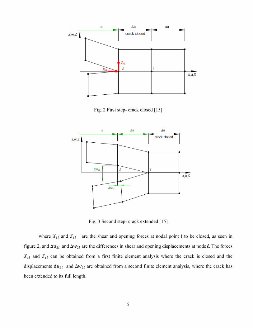
The two-step VCCT method is based on the assumption that energy released when the crack is
extended by ∆a from a (figure 2) to a + ∆a (figure 3) is identical to close the crack between location ł to
i. Index 1 in formula 8 denotes the first step and index 2 is the second step. For a two-step method the
energy required goes as follows:
∗ ∆ ∗ ∆ (8)
5
Fig. 2 First step- crack closed [15]
Fig. 3 Second step- crack extended [15]
where and are the shear and opening forces at nodal point ł to be closed, as seen in
figure 2, and ∆ and ∆ are the differences in shear and opening displacements at node ł. The forces
and can be obtained from a first finite element analysis where the crack is closed and the
displacements ∆ and ∆ are obtained from a second finite element analysis, where the crack has
been extended to its full length.

6
The VCCT is based on the same assumptions as the two-step VCCT, but the difference is that the
displacements behind the crack tip at node i, are approximately equal to the displacements behind the
original crack tip at node ł.
Fig. 4 One step-VCCT [15]
The energy released when the crack tip is extended by ∆ from ∆ to 2∆ is identical to
the energy required to close the crack between location i and k. The formula for VCCT is the following:
∗ ∆ ∗ ∆ (9)
where and are the shear and opening forces at nodal point i and ∆ and ∆ are the shear and
opening displacements at node ł as seen in figure 4. The forces and displacements required to calculate
the energy to close the crack may be obtained from one single element analysis.
The fracture criterion used for all the experiments that involved VCCT was the power law criterion.
The power law model is described by Wu [20] with the following formula:
(10)
where is the equivalent energy release rate, and is the critical energy release
rate. For using this fracture criteria, one must provide the critical energy release rate for the different
types of loadings and provide , , and , which are exponents used to decide if a linear or non-

7
linear model will be used. This is an empirical relation based on experimental observations by Wu, he
did the following statement: “The crack propagates along an essentially straight line but makes
microscopic skips across neighboring glass fibers." In his paper he proposed two approaches, but this
relationship fitted the data from the experiments he realized.
2.2.2 CZM
Although it is not part of this study, an introduction to CZM is offered because later, cohesive
segments will be introduced with X-FEM. CZM has gained considerable attention over the past decade,
as it represents a powerful yet efficient technique for computational fracture studies. The early
conceptual works related to CZM date back to the early 60's and were carried out by Barenblatt, who
proposed the CZM to study perfectly brittle materials and Dugdale, who adopted a fracture process zone
concept to investigate ductile materials exhibiting plasticity [18]. Cohesive zone elements do not
represent any physical material, but describe the cohesive forces which occur when material elements
are being pulled apart [11]. One of the advantages that cohesive elements present is that an initial flaw is
not needed, so cohesive elements are implanted at potential failure sites and are introduced a softening
traction/separation behavior, as seen in figure 5, allowing the onset of a crack when the criteria is met .
Fracture mechanics is indirectly introduced because the area under the softening curve is equated to the
critical fracture energy [12].
Fig. 5 Traction/displacement relationship [12]

8
Further reading is encouraged to get a better understanding of CZM, there are a lot of aspects in
this area that need special attention to do a proper cohesive zone modeling.
2.3 X-FEM
The extended finite element method (X-FEM) is a numerical technique that extends the classical
finite element method by enriching the solution space for solutions to differential equations with
discontinuous functions [2]. The extended finite element method was first introduced by Belytschko and
Black [8]. With X-FEM you can study the onset and crack propagation in quasi-static problems, one of
the advantages of the method, is that it allows you study crack growth along an arbitrary, solution-
dependent path without the needing to remesh the model [9].
For fracture analysis, the enrichment functions typically consist of the near-tip asymptotic
functions that capture the singularity around the crack tip and a discontinuous function that represents
the jump in displacement across the crack surfaces [2]. Approximation for a displacement vector
function u with the partition of unity enrichment is
∑ ∑ (11)
Where are the usual node shape functions; the first term on the right-hand side of the
above equation, is the usual node displacement vector associated with the continuous part of the finite
element solution; the second term is the product of the nodal enriched degree of vector, , and the
associated discontinuous jump function across the crack surfaces; and the third term is the product
of the nodal enriched degree of freedom vector, , and the associated elastic asymptotic crack-tip
functions, . Figure 6 gives a more clear understanding of formula number 11.

So in
sub-element
superposed
no longer tie
2.4
The
written as:
n other word
ts by additi
to the origin
ed together a
J-INTEG
J-integral w
ds, the crack
ional nodes
nal ones. Wh
and can mov
GRAL
was first intr
Fig. 6 X-
k can grow t
s. ABAQUS
hen the elem
ve apart.
roduced by R
9
-FEM conce
through the e
S call these
ment is cut th
Rice [17]. F
epts [2]
elements, el
e nodes ph
hrough the c
For a 2D con
ements that
hantom node
crack, real an
nfiguration,
are partition
es, which a
nd phantom
the J integr
ned create
are nodes
nodes are
ral can be
(12)

Here
sense startin
T is the trac
vector, and
The
around the c
Beca
criterion. Th
extent the r
plastic defor
e Г is a curv
ng from the l
ction vector d
ds is an elem
J-integral ca
crack tip [8].
J is a pa
J is equa
J is equa
J can ea
J can be
ause of the m
he propertie
ealm of app
rmation and
Fig. 7 Arb
ve surroundi
lower flat no
defined acco
ment of arc le
an be viewed
. The fundam
ath independ
al to
al to G
asily be deter
e related to th
mentioned p
es were deri
plicability of
possible sta
bitrary conto
ing the notch
otch surface
ording to the
ength along
d as a param
mental prope
ent for linea
for linear or
rmined expe
he crack tip
properties, J
ived under
f the J-integ
able crack gr
10
our path enc
h tip, the int
and continu
e outward no
Г.
meter which
erties of J are
ar or nonlinea
r nonlinear e
rimentally
opening disp
has been pro
elastic mate
gral fracture
rowth preced
losing the cr
tegral being
uing along th
ormal along
characterize
e the followi
ar elastic ma
elastic mater
placement δ
oposed as an
erial respons
criterion to
de fracture in
rack tip
g evaluated i
he path Г to t
Г, Ti=σijnj,
es the state o
ing:
aterial respon
rial response
n attractive
se. Attempts
ductile frac
nstability.
in a counterc
the upper fla
u is the disp
of affairs in t
nse
e
candidate fo
s have been
cture where
clockwise
at surface.
placement
the region
or fracture
n made to
extensive

11
3. METHODOLOGY
3.1 MODE I PROPAGATION
For modeling crack growth in mode I, a DCB specimen was chosen. The DCB is an attractive
configuration for the study of crack propagation and arrest, both from the experimental and theoretical
points of view [10], figure 8 shows the configuration of the specimen.
Fig. 8 Double cantilever beam specimen
The dimensions used in this study were the following:
a= 0.2 meters
b= 0.6 meters
2h= 0 .03 meters
B= 0.2 meters
The dimensions for this specimen were chosen randomly, only taking into account that the
dimensions for initial flaw, thickness, and length were valid within the range of linear elastic fracture
mechanics and a plane strain condition was present.
The dimensions requirement for this validation was obtained using the following equations:
2.5
(13)

12
2.5
(14)
2.5
(15)
These equations according to the American Society for Testing Materials (ASTM) [6], ensures
that the thickness requirement gives nearly plane strain conditions at the tip, while the on in-plane
dimensions ensure that the normal behavior is elastic and that characterizes crack tip conditions.
The material properties used for the model were chosen to mimic AISI 4340 steel; the stress
intensity factor is the only property that was modified to have a tougher material. There was no
special criterion for this property change other than see how a tougher metal behaved in the numerical
model. Table 1 shows the principal material properties used.
Table 1. Material properties of mode I specimen
Properties Value Units
Critical energy release rate 20000
Critical stress intensity factor 65000000 ∗ √
Elastic modulus of elasticity 200000000000
Yield strength 472000000
Now that the dimensions and the properties of the model had been introduced, the beam theory
used to benchmark ABAQUS is explained.
There is more than one analytical model for a DCB, one example is based on a linear elastic
foundation proposed by Kanninen [10], but for this study a simple beam theory without any type of
sophistication was used. In the recommendations section, other analytical solutions are discussed.
For the simple beam theory model, the two arms are considered as cantilevers with zero rotation
at its ends. With this assumption in mind, the equations used for the model were the following:

13
(16)
where 1 is used for plane strain; υ is the Poisson’s ratio
From this equation, variable a was the desired crack extension length and we solved for u in
order to find the displacement needed to increase the crack. For this study, the goal was to propagate the
crack 0.3 meters from the initial flaw making the complete crack length equal to 0.5 meters.
Once the displacement was found, it was important to consider that this displacement is not for
a single arm so:
(17)
when was found, simple beam theory was applied to get the force for the onset of crack
growth. This was done by using equation 18, where a needed to be the size of the initial flaw.
(18)
where is equal to:
(19)
Based on the dimensions and properties of the model, the necessary applied displacement to
growth the crack the desired amount was 0.049 meters.
Once the problem was defined, a 2D model was set-up in ABAQUS/STANDARD. An implicit
scheme was used with a mesh size of 0.001 meters, quadrilateral first order elements were used with the
formulation CPE4I. Figure 9 shows the mesh used for the simulation; 24,000 elements were created with
the mentioned mesh size, simulations with finer meshes were done, but the results were comparably
equal and the time consumed for a finer mesh analysis was greater with no extra benefit at all.

14
Fig. 9 Mesh used for mode I propagation
The initial step size was set to be .001, the minimum to be 1E-020, and a maximum of .001 was
used during the applied displacement step. For a VCCT analysis, small time increments are required.
ABAQUS track the location of the active crack front node by node; therefore the crack is allowed to
advance a single node at the time in any single increment. This is the reason why the initial and
maximum time step are so small; the same parameters for time step was used with the other two
techniques: X-FEM coupled with VCCT and X-FEM with cohesive segments.
The boundary conditions applied for this model are shown in figure 10; these boundaries are: the
applied displacement and a restriction in movement in the x-axis where the applied displacement is
located in order to prevent rotation. This configuration resembles the arrangement of the classical fixed
cantilever beam, where a displacement is applied at the free end and in the opposite side there is a wall.
Fig. 10 Applied boundary conditions

15
Now that the basic parameters for the model have been introduced, the set-up of the fracture
mechanics routines is presented.
3.1.1 VCCT
The VCCT as mentioned in chapter 2, is a technique that helps us simulate crack propagation. As
mentioned in [2], crack propagation problems using VCCT criterion are numerically challenging. In
order to help overcome convergence issues during the propagation, ABAQUS provides three different
types of damping to aid convergence for the model: contact stabilization, automatic stabilization and
viscous regularization. For this study, only viscous regularization was used based on the comments of
Ronald Krueger [14]. Viscous regularization in ABAQUS is based on a Duvaut-Lions regularization
scheme.
Viscous regularization is applied only to nodes on contact pairs that have just debonded. The
viscous regularization damping causes the tangent stiffness matrix of the softening material to be
positive for sufficiently small time increments, other reason why small time steps were used [2]. The
recommendation for use viscous regularization in models when convergence become difficult is to set
the damping parameters to relatively high values and rerun the analysis, for this study the parameters
were chosen based on a iterative procedure to see which values would help to converge the model.
When using viscous regularization, is necessary to monitor the energy absorbed by viscous damping,
this is done by checking the viscous damping ALLVD against the total stain energy in the model ALLSE,
the criterion used for this study was to ensure that no more that 3% of ALLVD vs. ALLSE was used.
Table 2 shows the values used and the results that were obtained.
Table 2. Damping parameters for mode I VCCT
VISCOUS REGULARIZATION CONVERGE STEP OF FAILIURE
None No 0.59
1E-06 Yes NA
1E-08 Yes NA

16
To model the initial flaw a, a seam line was used. The definition of seam crack according to
ABAQUS manual 6.11 is the following; "A seam defines an edge or a face with overlapping nodes that
can separate during an analysis." Figure 11 show a representation of a seam line:
Fig. 11 Seam Crack [2]
A master surface, slave surface, and a contact formulation need to be defined to perform a
VCCT analysis; for this study, a finite sliding, node to surface (default contact formulation) was used.
The mentioned aspects are the more relevant to the use of VCCT. Load/displacement plots are presented
in the next chapter.
3.1.2 X-FEM VCCT
For X-FEM coupled with VCCT, the set-up of the fracture mechanics routine was similar to
VCCT, one of the biggest advantages found was that the routine for X-FEM VCCT was more
straightforward to implement than VCCT. The difference between VCCT and X-FEM VCCT is that the
latter one can be used to simulate crack propagation along an arbitrary, solution-dependent path without
the requirement of a pre-existing crack in the model. The process used for model mode I propagation
consisted in specify three parameters: a crack domain, define crack growth, and the direction criterion
for growth. Figure 12 shows how ABAQUS presents the crack domain.

17
Fig. 12 X-FEM crack domain
Viscous regularization was used to assist convergence as the material fails. The damping
parameters used were similar as the ones for VCCT; viscous damping against total strain energy was
checked in order to ensure the model was correct. Table 3 shows the results obtained.
Table 3. Damping parameters for mode I X-FEM VCCT
VISCOUS REGULARIZATION CONVERGE STEP OF FAILIURE
None No 0.185
1E-06 Yes NA
1E-07 Yes NA
1E-08 No 0.186
For this model, the initial flaw was indicated in the model, but it wasn't modeled as in VCCT.
The pre-existing crack for X-FEM must be contained within the crack domain, also is important to point
out that a seam crack must not be used to specify the initial flaw, the program would give back an error
before it is submitted for analysis.
3.1.3 X-FEM COHESIVE SEGMENTS
X-FEM with cohesive segments was the other approach used with X-FEM; this method is based
on the traction separation cohesive behavior. One difference between X-FEM VCCT and X-FEM
cohesive segment is that the latter can be used for modeling brittle or ductile fracture whereas the X-
FEM VCCT is recommended for brittle fracture only. The set-up for this technique consisted in defining
the enriched area, as in the previous analysis, and the following criteria for crack growth: damage

18
initiation and damage evolution. For damage initiation and extension, ABAQUS uses the following built
in models:
the maximum principal stress criterion
the maximum principal strain criterion
the maximum nominal stress criterion
the maximum nominal strain criterion
the quadratic traction-interaction criterion
the quadratic separation-interaction criterion
The model used for this study was the maximum nominal stress criterion, which is represented by the following equation:
max⟨ ⟩
, , (20)
For this study, the nominal traction stress vector, t, consists of two components, tn is the
component normal to the likely cracked surface and ts is the shear component. tn and ts represent the
peak values of the nominal stress. Formula 21 shows the equation used for calculating the initiation
parameter for the normal traction of the crack surface.
√ (21)
For this formula we used r as the element size ahead the crack tip, the stress intensity factor was
a parameter given by the material property. The value damage initiation was 797810000Pa.
Once established the damage initiation, damage evolution was specified. Damage evolution describes
the rate at which the cohesive stiffness is degraded once the initiation criterion is met. For this study an
energy criterion was chosen, which is based on the dissipated energy as a result of the damage process.
The critical energy release specified in the previous analysis was chosen. A linear model was the used
as the one seen in figure 5.

19
Viscous regularization of the constitutive equations defining cohesive behavior in an enriched
element was used to help converge the model. Table 4 shows the results
Table 4. Damping parameters for mode I X-FEM COHESIVE SEGMENTS
VISCOUS REGULARIZATION CONVERGE STEP OF FAILIURE
None No 0.185
1E-05 Yes NA
1E-07 Yes NA
1-E08 No 0.185
3.2 MIXED MODE I/II PROPAGATION
The mixed mode crack growth was obtained by using a mixed-mode bending (MMB) specimen,
this configuration was first suggested by Reeder and Crews [16]. The test simply combines the mode I
DCB and the mode II end notch flexure specimen (ENF). The relative magnitude of the two applied
loads determines the mixed mode ratio at the propagation front. Figure 13 shows the configuration of the
MMB specimen.
Fig. 13 MMB specimen [19]

20
The dimensions and properties used for the MMB specimen were exactly the same ones as for
the DCB, only the addition of critical energy release rate GII is added to the model which had the same
value as GI. The goal as is to propagate the crack 0.4 meters from the initial flaw. To verify that the
crack had growth the desired amount, in the post-processing part of the analysis, a path was created from
the first node located in the initial flaw to the last node where the crack had stopped, figure XX shows
the path in the viewport. Beam theory was used to select the parameters for model the MMB in
ABAQUS, the approach followed is presented in the next paragraphs.
Fig. 14 Crack path

21
The MMB loading is represented by a superposition of simple mode I and mode II loadings
equivalent to those used with DCB and ENF. Figure 15 shows how the superposition procedure
incorporates beam theory equations.
Fig. 15 Superposition for mode I and mode II [16]
For this study the desired mixed mode ratio was set to be GII/Gt=0.5, where Gt equals GI + GII.
The loading position c determines the relative magnitude of the two resulting loads on the specimen and
therefore determines the mixed mode ratio, so the first step was to find the value of c for the desired
ratio.
The applied load distance, c, was based on Tenchev and Falzon paper [19]. The reason for use
their derivation is that the authors recognized that in previous publications, when the crack grows bigger
than L (as seen in figure 13), the mode separation used by Reeder and Crews is not valid anymore.
Based on this statement and considering that the desired crack growth goes beyond L, the proposed
equations used to get the length c for the desired mixed mode ratio are the following:
3 1 5 13 1 3 (22)
1 1 2 1 1 5 1 (23)
By knowing that the ratio must be GI/GII=1.0, we equate these two equations and set- up a to the
desired amount of crack growth and solve for c.

22
Once that c was found, a linear mode fracture criteria was used for solve for P, this fracture
criteria is essentially the power law.
1 (24)
The value of P for the MMB came to be 21,184 N. Once P is known, the values for P1 and P2
were obtained using following equations:
(25)
(26)
As mentioned in the mode I analysis, control displacement is preferred in order to avoid
numerical instabilities. The equations used to find out the displacement are shown next.
(27)
where a is the desired crack extension. Displacement d2 was not specified by Tenchev and
Falzon, but another study performed by Kinloch, Wang, Williams and Yayla [1], explain the method to
obtain the middle displacement by applying beam theory. The derived equation is the following:
1 (28)
where
2 1 2 (29)
7 1 (30)
(31)

23
The boundary condition used for the model consisted of a fixed pin in the opposite arm of to the
applied displacement, half length middle displacement in the y-axis and a roller in the opposite side
from the pin. Figure 16 shows the boundary conditions
Fig. 16 Boundary conditions for MMB
Now that the model has been set- up, ABAQUS implementation is presented.
3.2.1 VCCT
Implementation of VCCT for the MMB followed the same approach as in mode I. The difference
consisted that the parameter GII was defined in the fracture criterion. Viscous regularization was used,
table 5 shows the results
Table 5. Damping parameters for mixed mode I/II VCCT
VISCOUS REGULARIZATION
CONVERGE STEP OF FAILIURE
Release Tolerance
NLGEOM
None No 0.37 0.2 No 1E-02 No 0.39 0.2 No
1E-03 No 0.37 0.2 No
1E-02 No 0.44 0.5 Yes
1E-03 No 0.42 0.5 Yes
1E-04 No 0.42 0.5 Yes
From table 5 it was observed that none of the analysis converged, a lot more analysis were run
but here are presented the most representatives cases. One of the causes for this behavior might be the
criterion used for crack growth. In order to help converge the model, the release tolerance was modified,
it helped but the model in comparison to the default tolerance, but the model still did not converge.
Nonlinear geometry was activated as well in the model with greater release tolerance as indicated in

24
ABAQUS manual 6.11 to help converge the model but that didn’t help. Same parameters were applied
to X-FEM to see if there was any difficulty like the one with VCCT.
3.2.2 X-FEM VCCT
Same approach as in mode I. Viscous regularization results are shown in table 6.
Table 6. Damping parameters for mixed mode I/II X-FEM VCCT
VISCOUS REGULARIZATION CONVERGE STEP OF FAILIURE
None No 0.213
1E-06 Yes NA
1E-07 Yes NA
1E-08 No 0.18
1E-09 No 0.15
3.2.3 X-FEM COHESIVE SEGMENTS
Same approach as in mode I. Viscous regularization results are shown in table 7.
Table 7. Damping parameters for mixed mode I/II X-FEM COHESIVE SEGMENTS
VISCOUS REGULARIZATION CONVERGE STEP OF FAILIURE
None No 0.150
1E-05 Yes NA
1E-06 Yes NA
1E-07 No .153
3.3 J-INTEGRAL FOR ENERGY RELASE RATE CALCULATION
The energy release rate is an important parameter in fracture mechanics since we can relate it to
the stress intensity factor as seen in formula 5. In ABAQUS we can use the J-integral to calculate G
based on the statement that . The used methodology for this study is discussed next.

25
The specimen for this assessment was an infinite plate with an edge crack. The material
properties were the same as the ones used for crack growth with the exception of the critical stress
intensity factor, where 50000 √ . Figure 17 shows the edge crack specimen.
Fig. 17 Edge crack plate
where
a=0.03 meters
b=0.10 meters
B=0.05 meters
2h=0.20 meters
The boundary conditions and the loads used for this study are shown in figure 18. The boundary
conditions used were two nodes fixed in the x-axis to prevent any rotation at the tips of the edge where
the initial crack is located. A restriction in the y-axis in the middle of the edge opposite to the initial
crack was used to ensure a mode I reading.

26
For determine the remote stress applied to the plate, the following formula was used were some
proportions had to be met.
√ (32)
where
1 (33)
and
0.3 (34)
From formula 32, all the variables were known with the exception of . For this particular case,
after solving for σ, the obtained value was 97475000 .
Fig. 18 Load and boundary conditions for J-integral assessment

27
Once the geometry, boundary conditions, and load were defined, the next step was the set-up of
the contour integral analysis. The first step was to define the crack front. In a 2D analysis you can define
the crack front from the three following options: a single vertex, connected edges, and connected faces;
for this study the vertex option was selected.
The next step was to define crack tip; in which this case was the same vertex as in the crack
front. After having defined those two parameters, the subsequent procedure consisted in specifying the
crack extension. ABAQUS provides two options to specify the crack extension: normal to crack plane,
, or virtual crack extension direction, . For this study, the virtual crack extension was defined by
selecting the points from the model that represents the start and the end of the q vector, which were the
beginning of the crack and the node chosen as crack front respectively. Figure 19 shows how the
direction is represented in the viewport.
Fig. 19 q vectors

28
Now that the model parameters had been defined in the analysis, we have to mesh the geometry.
For this analysis it was important to create the singularity in the mesh to improve the accuracy of the J-
integral. Since linear elasticity is used, the singularity to capture is √
. To create the square root
singularity, we need to constrain the nodes on the collapsed face of the edge to move together and move
the nodes to the 1/4 points. Figure 20 shows a representation of a 2D collapsed element and figure 21
shows the actual mesh used.
Fig. 20 Collapsed two dimensional element [2]
Fig. 21 Mesh used for J-integral study

29
An implicit scheme was selected with the default time step: 1 for initial and maximum, and a
minimum of 1E-05. The element selection was CPE8 based on the plane strain assumption mentioned
earlier and the quadratic formulation was used to collapse one side of the element as previously
explained.

30
4. RESULTS
4.1 MODE I LOAD/DISPLACEMENT PLOTS
Figure 22 and 23 show the DCB in the post-processing part of the analysis in ABAQUS.
Fig. 22 DCB model in ABAQUS
Fig. 23 Von Mises stress at the crack tip

31
4.1.1 VCCT PLOT
Fig. 24 Mode I VCCT load/displacement plot
Figure 24 shows the load/displacement plot for VCCT. As seen, the necessary load for initiate
the crack from the analytical model is 31,997 N and from the numerically model the load obtained was
33,855 N, the difference is about 5% off from the analytical model. This solution is consistent to the
solution found by Crews and Reeder [16]. This plot gives us the confidence that the implemented VCCT
routine in ABAQUS is accurate since is giving us the same approximations as found by different authors
in previous experiments.

32
Fig. 25 Pattern difference using different viscosity for VCCT
A saw tooth pattern is seen in the plot, according to Ronald Krueger [14], this behavior appears
to be dependent on the mesh size at the front of the crack. From this plot is concluded that the viscosity
1E-08 attenuate the saw tooth pattern.

33
4.1.2 X-FEM VCCT PLOT
Fig. 26 Mode I X-FEM VCCT load/displacement plot

34
Figure 26 shows the load/displacement plot for X-FEM VCCT. As seen, the necessary load for
initiate the crack from the analytical model is 31,997 N and from the numerically model the load
obtained was 35,103 N, the difference is about 9% off from the analytical model. As explained earlier,
this solution has the average offset seen in previous works, but an important difference is that in
previous works only VCCT was used, a similar study were X-FEM VCCT was used was not found
Fig. 27 Pattern difference using different viscosities for X-FEM VCCT
The saw tooth pattern is stronger with X-FEM VCCT than with VCCT.

35
4.1.3 X-FEM COHESIVE SEGMENTS
Fig. 28 Mode I X-FEM COHESIVE SEGMENTS load/displacement plot
Figure 28 shows the load/displacement plot for X-FEM VCCT. As seen, the necessary load for
initiate the crack from the analytical model is 31,997 N and from the numerically model the load
obtained was 34,917 N, the difference is about 9% off from the analytical model.

36
Fig. 29 Pattern difference using different viscosities for X-FEM COHESIVE SEGMENTS
Figure 29 shows the saw tooth pattern for a viscosity of 1E-06, but the following value of 1E-05 shows a totally different pattern than ones seen.

37
4.1.4 COMPARISON OF THE THREE TECHNIQUES
Fig. 30 Plot showing the three different techniques used.
Figure 30 shows how the initial load for delamination for both X-FEM approaches required more
force than VCCT. Also is seen how X-FEM VCCT and X-FEM COHESIVE SEGMENTS have a
similar pattern at the moment of crack growth. In the recommendations section, future work that can
help to fit the numerical model to the closed-form analytical solution will be discussed.

38
4.2 MIXED MODE I/II LOAD/DISPLACEMENT PLOTS
Figure 31 and 32 show the MMB in the post-processing part of the analysis in ABAQUS
Fig. 31 MMB specimen in ABAQUS
Fig. 32 Von Mises stress at the crack tip

39
4.2.1 X-FEM VCCT PLOT
Fig. 33 Mode I/II X-FEM VCCT load/displacement plot
Figure 33 shows the load/displacement plot for X-FEMVCCT. As seen, the necessary load for
initiate the crack from the analytical model is 32,019 N and from the numerically model the load
obtained was 44,738 N, the difference is about 39% off from the analytical model. Further investigation
is needed to decide if this percentage off comes from the numerical or analytical model.

40
Fig. 34 Pattern difference using different viscosities for X-FEM VCCT
Same saw tooth pattern is seen in mixed mode as seen in mode I propagation, figure 34 focuses
in the pattern created by using two different viscous values.

41
4.2.2 X-FEM COHESIVE SEGMENTS PLOT
Fig. 35 Mode I/II X-FEM COHESIVE SEGMENTS load/displacement plot
Figure 35 shows the load/displacement plot for X-FEMVCCT. As seen, the necessary load for
initiate the crack from the analytical model is 32,019 N and from the numerically model the load
obtained was 45,644 N, the difference is about 42% off from the analytical model. Further investigation
is needed to decide if this percentage off comes from the numerical or analytical model

42
Fig. 36 Pattern difference using different viscosities for X-FEM VCCT

43
4.2.3 COMPARISON OF THE TWO TECHNIQUES
Fig. 37 Plot showing the two different techniques used.
The two techniques used are shown in figure 37, as in the previous study for mode I, X-FEM
with cohesive segments needs a bigger load to star the crack based on the criterion used rather than X-
FEM VCCT. For future work is needed to decrease the percentage off the model, options to accomplish
this could be to use a quadratic power criterion, use BK criterion for fracture, and examine other option
of beam theory.

44
4.3 J-INTEGRAL RESULTS
The results obtained from the contour analysis were close the analytical solution. Based on
formula 5, the critical energy release rate for the specimen was 12500 . The results obtained
from the analysis are presented in figure 38, 10 contours were chosen and the result obtained after the
third contour is 11241 , which was the value used to compare against the analytical solution.
This gives us an offset of 10% to the closed-form solution which is in good approximation. Figure 39
shows the opening of the crack once the remote stress is applied.
Fig. 38 Results from data file
Fig. 39 Edge crack opening

45
5. CONCLUSION
In conclusion, ABAQUS capabilities for crack growth and calculation of energy release rate are
accurate to certain degree against the closed-form analytical solutions as seen in the results section. The
percentage off from the MMB is the one farther from the analytical solution. Crack growth in mode I
and energy release rate analysis gave decent solution when compared to the analytical ones. As
mentioned before, most of the work in crack growth analysis consisted in an iterative procedure, since
converging was very difficult to obtain. It is important to mention that from all the techniques,
implementing the routine of VCCT was the most difficult one. ABAQUS is not very user friendly at the
moment of defining the master surface, slave surfaces, and the nodes of the slave surface, one have to go
to the input file and create the node set and define the element edges for the surfaces manually. The
energy release rate calculation challenge was to generate the mesh to create the singularity; defining the
model parameters was straightforward. The techniques presented are a portion of the capabilities that
ABAQUS has for fracture mechanics, but they are the foundation for more complex models.

46
6. RECOMMENDATIONS FOR FUTURE WORK
If a closed-form analytical approach is used to benchmark ABAQUS, some recommendations
are given in order to assess ABAQUS further. For mode I propagation is recommended that the
analytical model from introduced by Kanninen [10]. He recognized that simple beam theory did not
properly model the interaction between the two arms of the DCB. The arms are not fixed against rotation
at the crack tip; they rotate slightly due to the elastic support they provide one another. By using this
analytical model, closer values to the ones obtained in the numerical model are expected. For mixed
mode bending I/II, different ratios should be studied as well. A paper by Turon and Costa [18] gives a
direct method to calculate c as the one used in this study. The ASTM standard for MMB testing [13]
proposes to find c in an iterative solution procedure, Turon and Costa proposed the following formula to
avoid the iterative procedure:
√ (35)
Variables and are explained in detail in the paper.
Validation against experimental results is encouraged since analytical models sometimes cannot
capture all the complexity of the fracture process.

47
REFERENCES
1. A.J. Kinloch, Y. Wang, J.G. Williams, P. Yayla, The mixed-mode delamination of fibre
composite materials, Composites Science and Technology, Volume 47, Issue 3, 1993, Pages
225-237, ISSN 0266-3538
2. Abaqus Analysis User’s Manual, ABAQUS® Standard, Version 6.11, DSS Simulia, 2011.
3. Anderson, Ted L. Fracture Mechanics: Fundamentals and Applications. Boca Raton: CRC Press,
1991. Print
4. ASTM D 6671-01, Standard Test Method for Mixed Mode I-Mode II Interlaminar Fracture
Toughness of Unidirectional Fiber Reinforced Polymer Matrix Composites, in Annual Book of
ASTM Standards, vol. 15.03: American Society for Testing and Materials, 2000
5. Belytschko, T., and T. Black, “Elastic Crack Growth in Finite Elements with Minimal
Remeshing,” International Journal for Numerical Methods in Engineering, vol. 45, pp. 601–620,
1999.Commercial Finite Element Codes," NASA/TM-2008-215123, 2008.
6. E 399-83, “Standard Test Method for Plane-Strain Fracture Toughness of Metallic Materials.”
American Society for Testing and Materials, Philadelphia, 1983.
7. E. F. Rybicki and M. F. Kanninen, A Finite Element Calculation of Stress Intensity Factors by a
Modified Crack Closure Integral, Eng. Fracture Mech., Vol. 9, pp. 931-938, 1977.
8. Gdoutos, E. E. (2005). Fracture mechanics an introduction. Dordrecht, Springer.
9. Ingraffea A R. Computational Fracture Mechanics. Volume 2, Chapter 11, Encyclopedia of
Computational Mechanics, E. Stein, R. de Borst, T. Hughes (eds.) John Wiley and Sons, 2004,
2nd Edition 2008.
10. Kanninen, M. F., “An Augmented Double Cantilever Beam Model for Studying Crack
Propagation and Arrest,” International Journal of Fracture, Vol.9, No.1, March 1973, pp.83-92.
11. Kregting, Rene, Cohesive Zone Models Toward a Robust Implementation of Irreversible
Behavior. 2005
12. Mi, U., Crisfield, M.A., Davies, G.A.O., Progressive delamination using interface elements.
Journal of Composite Materials, 32, 1246-1272, 1998.

48
13. N. Blanco, A. Turon, J. Costa, An exact solution for the determination of the mode mixture in
the mixed-mode bending delamination test, Composites Science and Technology, Volume 66,
Issue 10, August 2006, Pages 1256-1258, ISSN 0266-3538
14. R. Krueger, "An Approach to Assess Delamination Propagation Simulation Capabilities in
15. R. Krueger. Virtual Crack Closure Technique: History, Approach and Applications, Applied
Mechanics Reviews, vol. 57, pp. 109-143, 2004.
16. Reeder JR, Crews Jr JH. Mixed-mode bending method for delamination testing. AIAA J 1990;
28(7):1270–6.
17. Rice, J.R.: A Path Independent Integral and the Approximate Analysis of Strain Concentration
by Notches and Cracks, Journal of Applied Mechanics, 35 (1968), p. 379-386
18. Seong Hyeok Song, Glaucio H. Paulino, William G. Buttlar, A bilinear cohesive zone model
tailored for fracture of asphalt concrete considering viscoelastic bulk material, Engineering
Fracture Mechanics, Volume 73, Issue 18, December 2006, Pages 2829-2848, ISSN 0013-7944
19. Tenchev, RT & Falzon, BG 2007, 'A correction to the analytical solution of the mixed-mode
bending (MMB) problem' Composites Science and Technology, vol 67, no. 3-4, pp. 662-668.
20. Wu, E. M., and R. C. Reuter Jr., “Crack Extension in Fiberglass Reinforced Plastics,” T and M
Report, University of Illinois, vol. 275, 1965.

49
APPENDIX A. PARAMETERS FOR MMB

50

51
APPENDIX B. MODE I VCCT ROUTINE

52
APPENDIX C. MODE I XFEM-VCCT ROUTINE

53
APPENDIX D. MODE I XFEM-COHESIVE SEGMENTS ROUTINE

54
APPENDIX E. MIXED MODE I/II XFEM-VCCT ROUTINE

55
APPENDIX F. MIXED MODE I/II XFEM-COHESIVE SEGMENTS ROUTINE

56
VITA
Luis A. Hernández was born in Chihuahua, Chihuahua, México. He enrolled at the University of
Texas at El Paso in fall 2004 where he received his Bachelor of Science in Mechanical Engineering in
2009; afterwards he worked in the industry as a components engineer. In the spring of 2012 he decided
to pursue his Master of Science degree in Mechanical Engineering at the University of Texas at El Paso.
In summer 2013, he obtained his Master of Science degree.
Permanent address: 299 King’s Point Dr
El Paso, TX 79912
This thesis/dissertation was typed by Luis A. Hernandez.