Embed Size (px)
Citation preview
ABAQUS
Tutorial
Version 7.4
Fracture Analysis Consultants, Inc
www.fracanalysis.com
Revised: August 2019
2
Table of Contents:
1.0 Introduction .......................................................................................................................... 4
2.0 Tutorial 1: Crack Insertion and Growth in a Cube .............................................................. 5
2.1 Step 1: Create the ABAQUS FE Model .......................................................................... 6
2.2 Step 2: Reading ABAQUS FE Model into FRANC3D .................................................. 8
Step 2.1: Importing Complete ABAQUS FE Model .............................................................. 8
Step 2.2: Select the Retained Items in the FE Model ............................................................. 9
Step 2.3: Displaying the FE Model ....................................................................................... 12
2.3 Step 3: Importing and Subdividing the Model ............................................................... 13
2.4 Step 4: Insert a Crack ..................................................................................................... 19
Step 4.1: Define a new Crack from FRANC3D Menu ......................................................... 19
Step 4.2: Insert Cracks from Files......................................................................................... 24
2.5 Step 5: Static Crack Analysis ........................................................................................ 27
Step 5.1: Select Static Crack Analysis .................................................................................. 27
Step 5.2: Select FE Solver .................................................................................................... 29
Step 5.3: Select ABAQUS Analysis Options ....................................................................... 29
2.6 Step 6: Compute Stress Intensity Factors ...................................................................... 31
2.7 Step 7: Manual Crack Growth ....................................................................................... 33
Step 7.1: Select Grow Crack Rule ........................................................................................ 33
Step 7.2: Specify Fitting and Extrapolation .......................................................................... 36
Step 7.3: Specify Crack Front Template ............................................................................... 38
2.8 Step 8: Automatic Crack Growth .................................................................................. 39
Step 8.1: Open FRANC3D Restart File ................................................................................ 39
Step 8.2: Select Crack Growth Analysis ............................................................................... 40
Step 8.3: Specify Growth Rules ............................................................................................ 41
Step 8.4: Specify Fitting and Template Parameters .............................................................. 43
Step 8.5: Specify Growth Plan .............................................................................................. 43
Step 8.6: Specify Analysis Code ........................................................................................... 44
2.9 Step 9: SIF History and Fatigue Life ............................................................................ 46

3
Step 9.1: Select SIFs Along a Path ....................................................................................... 47
Step 9.2: Select SIFs For All Fronts ..................................................................................... 49
Step 9.3: Select Fatigue Life Predictions .............................................................................. 49
2.10 Step 10: Resume Growth with Larger Submodel ...................................................... 59
Step 10.1: Extract and Save Crack Geometry ...................................................................... 59
Step 10.2: Restart from Saved Crack Geometry .................................................................. 60
Step 10.3: Combine SIF Histories ....................................................................................... 65
Appendix A: ABAQUS local model defined between *Tie constraints...................................... 71
Appendix B: ABAQUS model with *Tied solid and shell meshes .............................................. 81
Appendix C: ABAQUS Initial Stress versus Crack Face Tractions ............................................. 87
C.1 ABAQUS Residual Stress ................................................................................................. 87
C.2 Residual Stress as Initial Stress ......................................................................................... 90
C.3 Residual Stress Included in FRANC3D ............................................................................ 93

4
1.0 Introduction
This tutorial introduces the fracture simulation capabilities of FRANC3D Version 7.4 and
ABAQUS Version 6.14 (earlier or later versions of ABAQUS should work also). The
FRANC3D software is introduced by analyzing a simple surface crack in a cube.
Subsequent tutorials (see the FRANC3D Tutorials #2-10 document) build on this first example
and describe additional capabilities and features of the software. It is intended that the user
perform the operations as they are presented, but you should feel free to experiment, and you
should consult the other reference documentation whenever necessary.
FRANC3D menu and dialog button selections are indicated by bold text, such as the File menu.
Window regions along with dialog options, fields and labels are underlined. Model names and
file names are indicated by italic text.
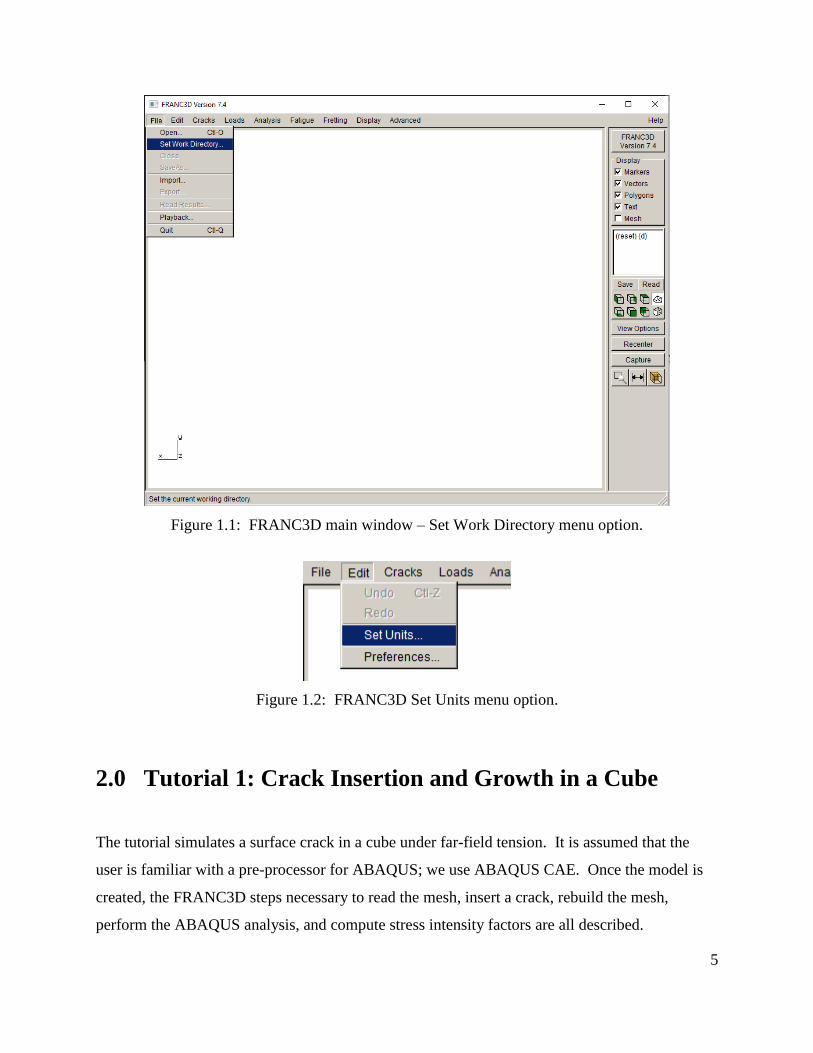
The FRANC3D main window is shown in Fig 1.1. When you start the tutorial, the first thing to
do is set the working directory using the File and Set Work Directory menu option, Fig 1.1.
After a model is imported, you can set the finite element model (FEM) units, Fig 1.2. The units
are applied to plots and figures that FRANC3D displays, and are used during crack growth. You
can also set your preferences; specifically, it is best to set the path to the ABAQUS executable.
You can view the preferences using the Edit and Preferences menu option. The Preferences
dialog is described in Section 5.4 of the FRANC3D Reference document.
5
Figure 1.1: FRANC3D main window – Set Work Directory menu option.
Figure 1.2: FRANC3D Set Units menu option.
2.0 Tutorial 1: Crack Insertion and Growth in a Cube
The tutorial simulates a surface crack in a cube under far-field tension. It is assumed that the
user is familiar with a pre-processor for ABAQUS; we use ABAQUS CAE. Once the model is
created, the FRANC3D steps necessary to read the mesh, insert a crack, rebuild the mesh,
perform the ABAQUS analysis, and compute stress intensity factors are all described.

6
2.1 Step 1: Create the ABAQUS FE Model
First, create a cube model using any pre-processor for ABAQUS. Here we simply outline the
necessary steps to create the model with boundary conditions to ensure that you have a complete
model that can be used with FRANC3D.
1. Create a 10x10x10 cube geometry; assume units of length are mm.
2. Subdivide the edges for meshing using 10 to 20 subdivisions.
3. Define the element type as quadratic elements; use brick or tetrahedral elements.
4. Define the material properties as 10000 for the elastic modulus and 0.3 for the Poisson’s
ratio; assume the units for E are MPa.
5. Mesh the volume.
6. Boundary conditions consist of displacement constraints on the bottom surface and
uniform traction (a negative pressure) on the top surface of 10 MPa. The bottom surface
is constrained in the y-direction, the bottom left edge is also constrained in the x-
direction, and the point at the origin is also constrained in the z-direction. Note that you
should use unique set and surface names when defining boundary conditions.
7. Save the model as an .inp file (Abaqus_Cube.inp).
The resulting model should appear as in Fig 2.1. The symbols for the boundary conditions are
displayed attached to the model; the brick mesh is displayed in the lower right corner.

7
Figure 2.1: ABAQUS cube with boundary conditions; meshed with brick elements.
Note that ABAQUS CAE uses default set and surface names such as SET-1 at both the Part and
Instance levels, Fig 2.1b, and the Instance SET-1 can be both a node and element set. If
boundary conditions are applied in CAE using the Instance SET-1 (right side image), FRANC3D
might apply the boundary conditions to both Part and Instance SET-1 nodes.
The solution is to name sets and surfaces in CAE with unique names, especially when defining
boundary conditions.

8
Figure 2.1b: ABAQUS CAE set-1 at both Part and Instance levels.
2.2 Step 2: Reading ABAQUS FE Model into FRANC3D
Start by importing an existing volume element mesh into FRANC3D. We use the
Abaqus_Cube.inp file from ABAQUS CAE, which was written in the previous step.
You can choose to do either Step 2 or Step 3 (Section 2.3); we describe both, but we use Step 3
for subsequent steps of this tutorial.
Step 2.1: Importing Complete ABAQUS FE Model
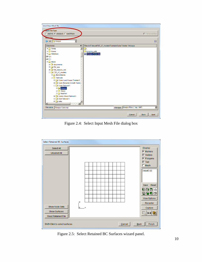
Start with the FRANC3D graphical user interface and select File and Import, Fig 2.2. In the
dialog shown in Fig 2.3, choose Complete Model. Switch the Mesh File Type radio button in the
Select Import Mesh File window, Fig 2.4, to ABAQUS and select the file name for the model,
called Abaqus_Cube.inp, Fig, 2.4. Select Next.
The mesh file type can be set in the Preferences so that you do not have to change the mesh file
type radio button if you always use ABAQUS.

9
Figure 2.2: FRANC3D graphical user interface
Figure 2.3 Import type
Step 2.2: Select the Retained Items in the FE Model
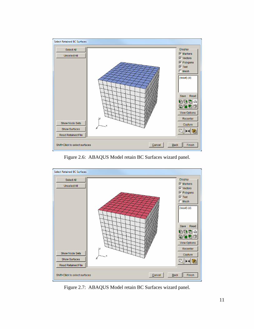
The next panel, Fig 2.5, allows you to choose the mesh surface facets that are retained from the
ABAQUS .inp file. Surfaces with boundary conditions appear as blue, Fig 2.6, and turn red
when selected, Fig 2.7. You can rotate the model to view all of the surfaces. We retain the
surfaces with boundary conditions (top and bottom of the cube) by choosing Select All. The
boundary conditions will be transferred automatically to the new mesh when a crack is inserted.
Select Finish to proceed.
10
Figure 2.4: Select Input Mesh File dialog box
Figure 2.5: Select Retained BC Surfaces wizard panel.
11
Figure 2.6: ABAQUS Model retain BC Surfaces wizard panel.
Figure 2.7: ABAQUS Model retain BC Surfaces wizard panel.
12
Surface Mesh NOT Retained
The surface mesh facets do not have to be retained, and if a crack will be inserted into a surface
that has boundary conditions, then the surface mesh must not be retained. In such a case, the
boundary condition data is mapped to the remeshed surface. In practice, transfer of boundary
condition data is simpler and more precise if the surface mesh can be retained, but sometimes
this is not possible; FRANC3D will automatically map the boundary condition data to the new
mesh regardless.
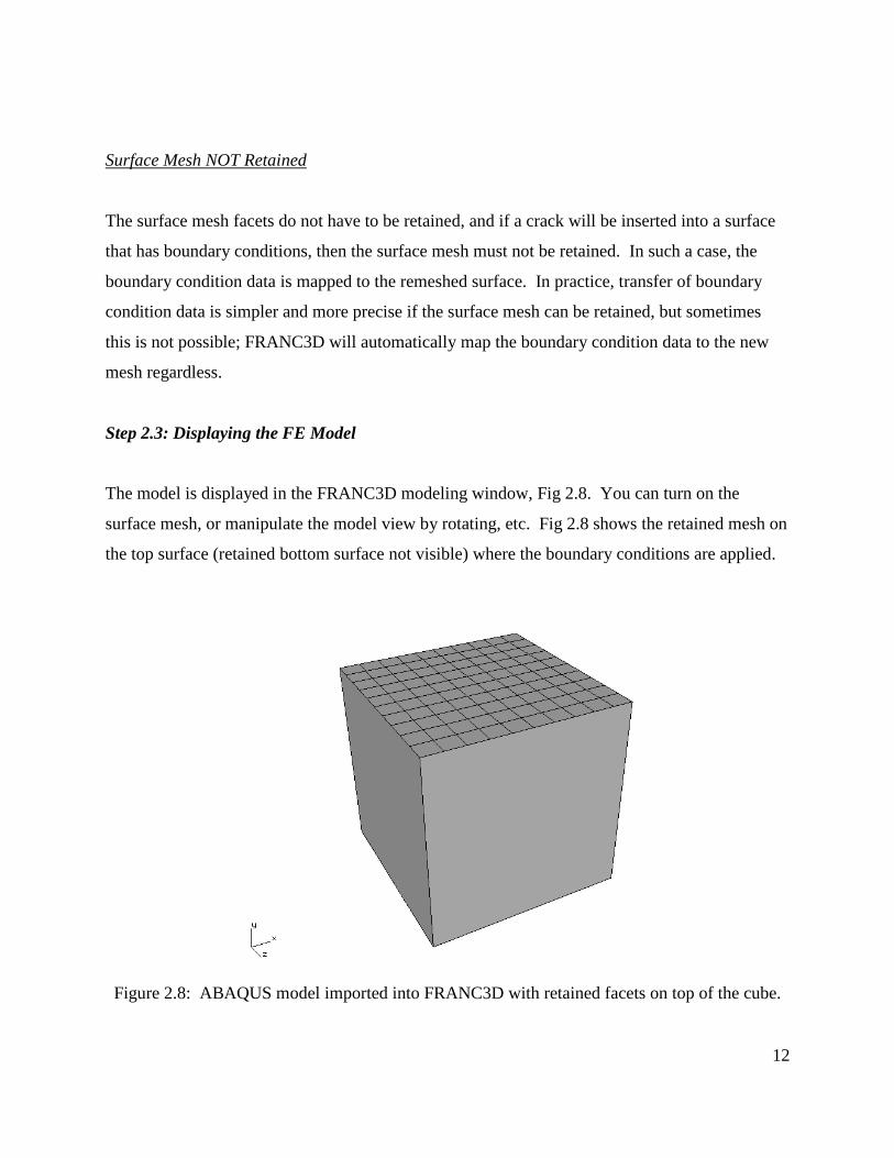
Step 2.3: Displaying the FE Model
The model is displayed in the FRANC3D modeling window, Fig 2.8. You can turn on the
surface mesh, or manipulate the model view by rotating, etc. Fig 2.8 shows the retained mesh on
the top surface (retained bottom surface not visible) where the boundary conditions are applied.
Figure 2.8: ABAQUS model imported into FRANC3D with retained facets on top of the cube.

13
If you have not set a working directory (using the File - Set Work Directory menu option),
FRANC3D might present the dialog shown in Figure 2.9 prior to displaying the model. Select
Yes to set the directory to be the folder where the ABAQUS .inp file resides. Quite a large
number of files are created during a crack growth simulation, and it is best to keep them all
together in a single folder.
Figure 2.9: Set Working Directory dialog.
2.3 Step 3: Importing and Subdividing the Model
If you chose to do Step 2 above, either skip this step, or close the model using the File - Close
menu option before starting this step.
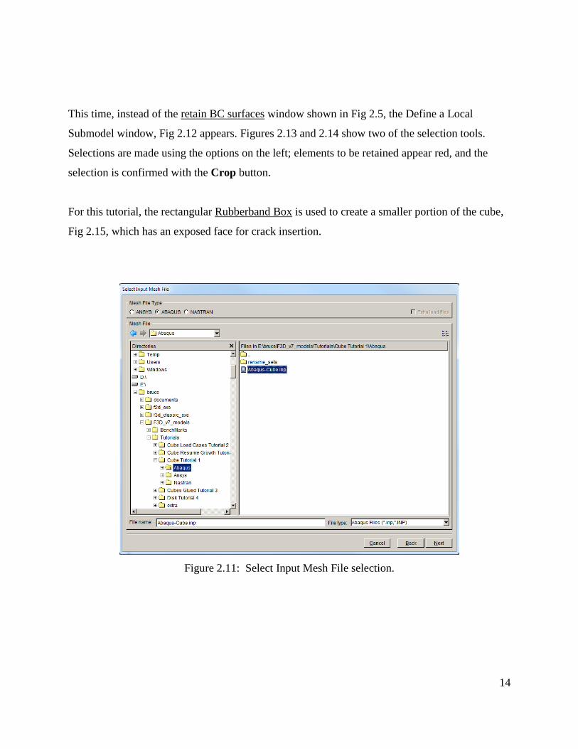
The ABAQUS model can be split into smaller parts before inserting the crack. Go to File and
Import, and choose the Import and divide into global and local models radio button, Fig 2.10,
and choose the Abaqus_Cube.inp model, Fig 2.11, as before. Remember to set the Mesh File
Type radio button to ABAQUS.
Fig 2.10 Import options
14
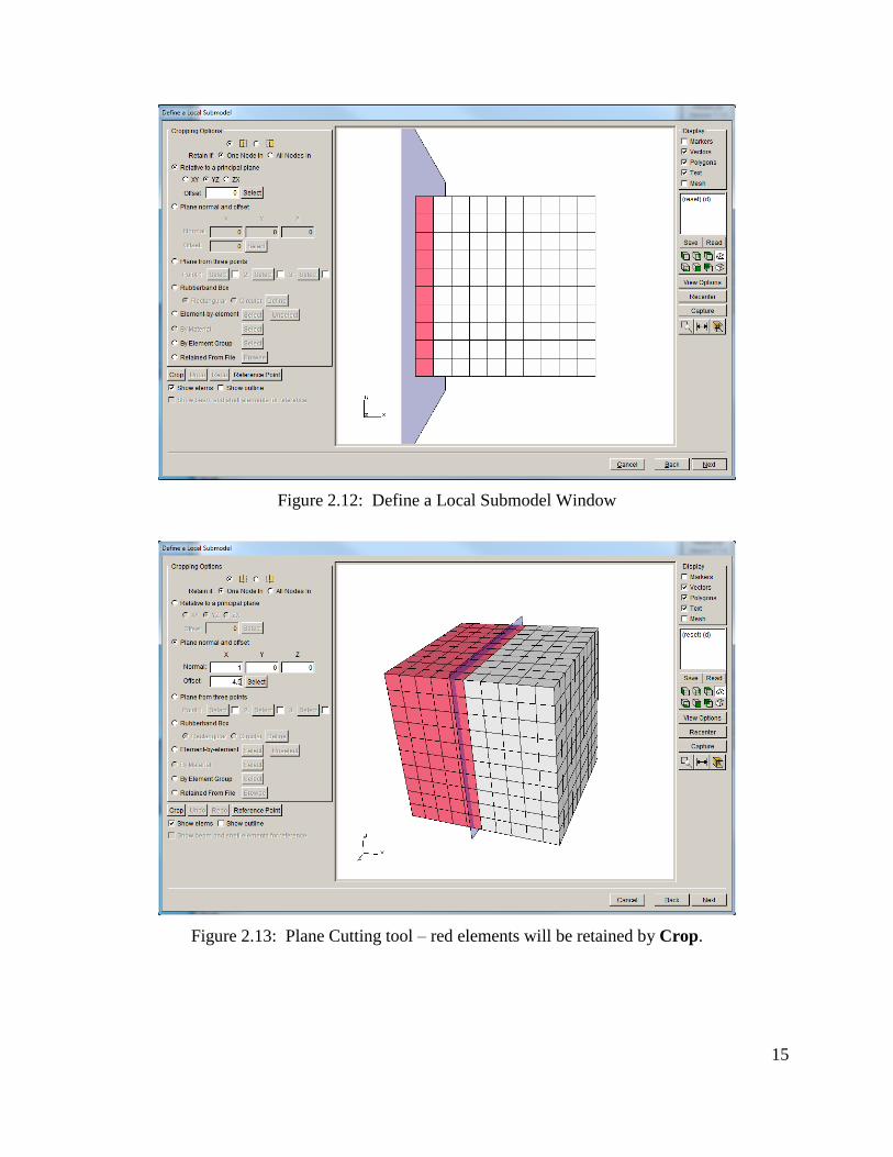
This time, instead of the retain BC surfaces window shown in Fig 2.5, the Define a Local
Submodel window, Fig 2.12 appears. Figures 2.13 and 2.14 show two of the selection tools.
Selections are made using the options on the left; elements to be retained appear red, and the
selection is confirmed with the Crop button.
For this tutorial, the rectangular Rubberband Box is used to create a smaller portion of the cube,
Fig 2.15, which has an exposed face for crack insertion.
Figure 2.11: Select Input Mesh File selection.
15
Figure 2.12: Define a Local Submodel Window
Figure 2.13: Plane Cutting tool – red elements will be retained by Crop.
16
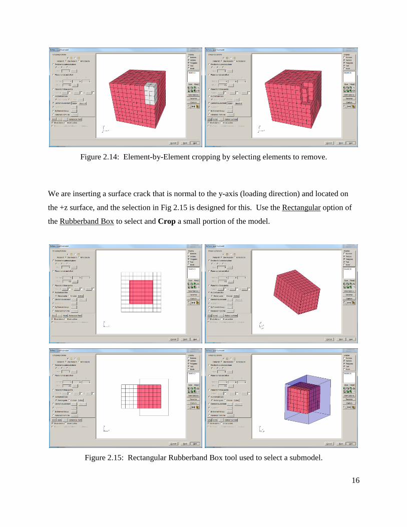
Figure 2.14: Element-by-Element cropping by selecting elements to remove.
We are inserting a surface crack that is normal to the y-axis (loading direction) and located on
the +z surface, and the selection in Fig 2.15 is designed for this. Use the Rectangular option of
the Rubberband Box to select and Crop a small portion of the model.
Figure 2.15: Rectangular Rubberband Box tool used to select a submodel.
17
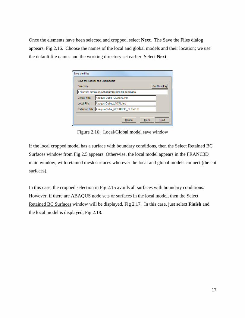
Once the elements have been selected and cropped, select Next. The Save the Files dialog
appears, Fig 2.16. Choose the names of the local and global models and their location; we use
the default file names and the working directory set earlier. Select Next.
Figure 2.16: Local/Global model save window
If the local cropped model has a surface with boundary conditions, then the Select Retained BC
Surfaces window from Fig 2.5 appears. Otherwise, the local model appears in the FRANC3D
main window, with retained mesh surfaces wherever the local and global models connect (the cut
surfaces).
In this case, the cropped selection in Fig 2.15 avoids all surfaces with boundary conditions.
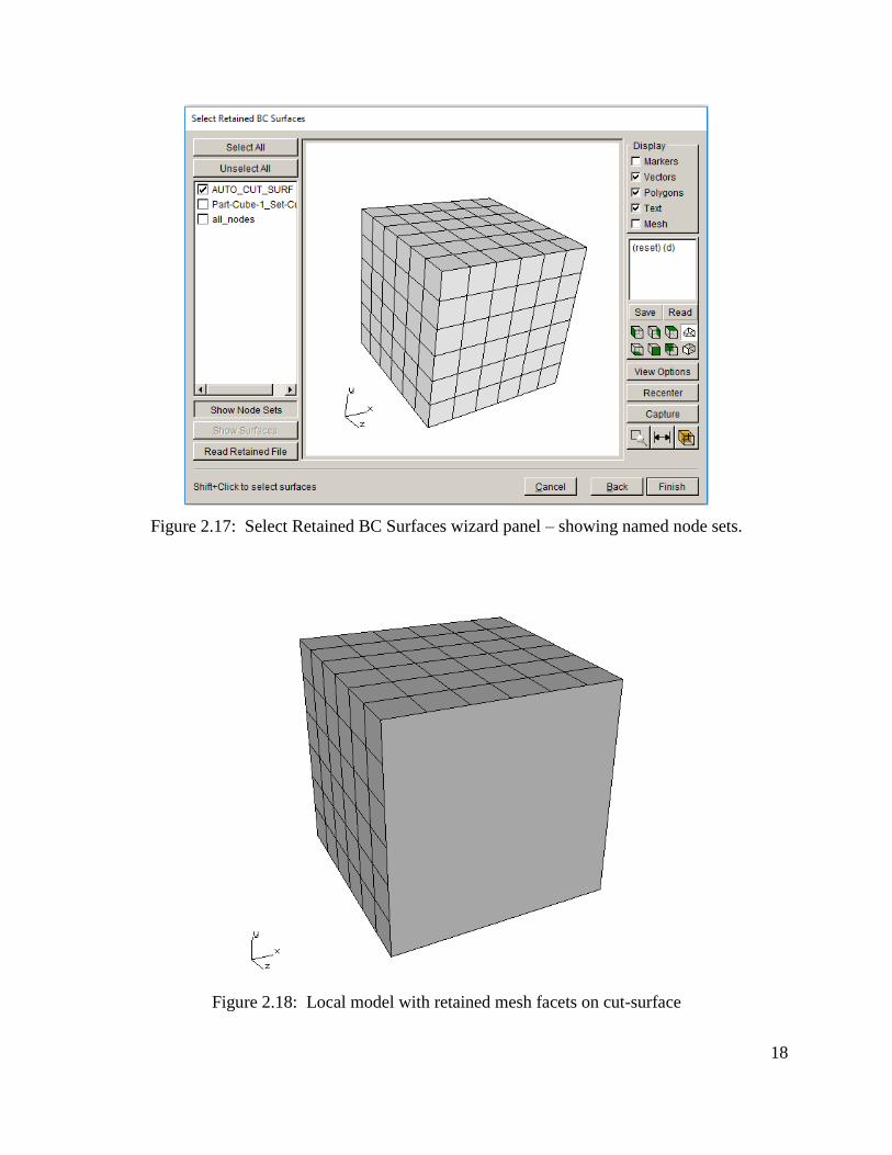
However, if there are ABAQUS node sets or surfaces in the local model, then the Select
Retained BC Surfaces window will be displayed, Fig 2.17. In this case, just select Finish and
the local model is displayed, Fig 2.18.
18
Figure 2.17: Select Retained BC Surfaces wizard panel – showing named node sets.
Figure 2.18: Local model with retained mesh facets on cut-surface

19
2.4 Step 4: Insert a Crack
We now insert a half-penny surface crack into the model. The local submodel from Section 2.3 is
used, as opposed to the full model. In Step 4.1, we describe how to define a new crack, and in
Step 4.2, we describe how to insert a flaw from a file. Note that you should not try to re-insert a
crack into a cracked model. Step 4.2 is described here and will be used in subsequent tutorials.
Step 4.1: Define a new Crack from FRANC3D Menu
From the FRANC3D menu, select Cracks and New Flaw Wizard as seen in Fig 2.19. The first
panel of the wizard should appear as in Fig 2.20. The flaw being added is a crack with zero
volume. We select the Save to file and add flaw radio button to save the file for subsequent
tutorials. Select Next. The second panel of the wizard, Fig 2.21, lets you choose the crack
shape; the default is the ellipse, which is what we want. Select Next.
Figure 2.19: New Flaw Wizard menu item selected.

20
Figure 2.20: New Flaw Wizard first panel – Crack (zero volume flaw) selected.
Figure 2.21: New Flaw Wizard second panel – choose ellipse shape.

21
The crack is a circle with radius=1, centered on the cube’s front (+z) face, and parallel to the xz-
plane (normal to y). The third wizard panel lets you set the dimensions for the ellipse, Fig 2.22;
set a=1 and b=1. Select Next.
Figure 2.22: New Flaw Wizard third panel – set ellipse dimensions.
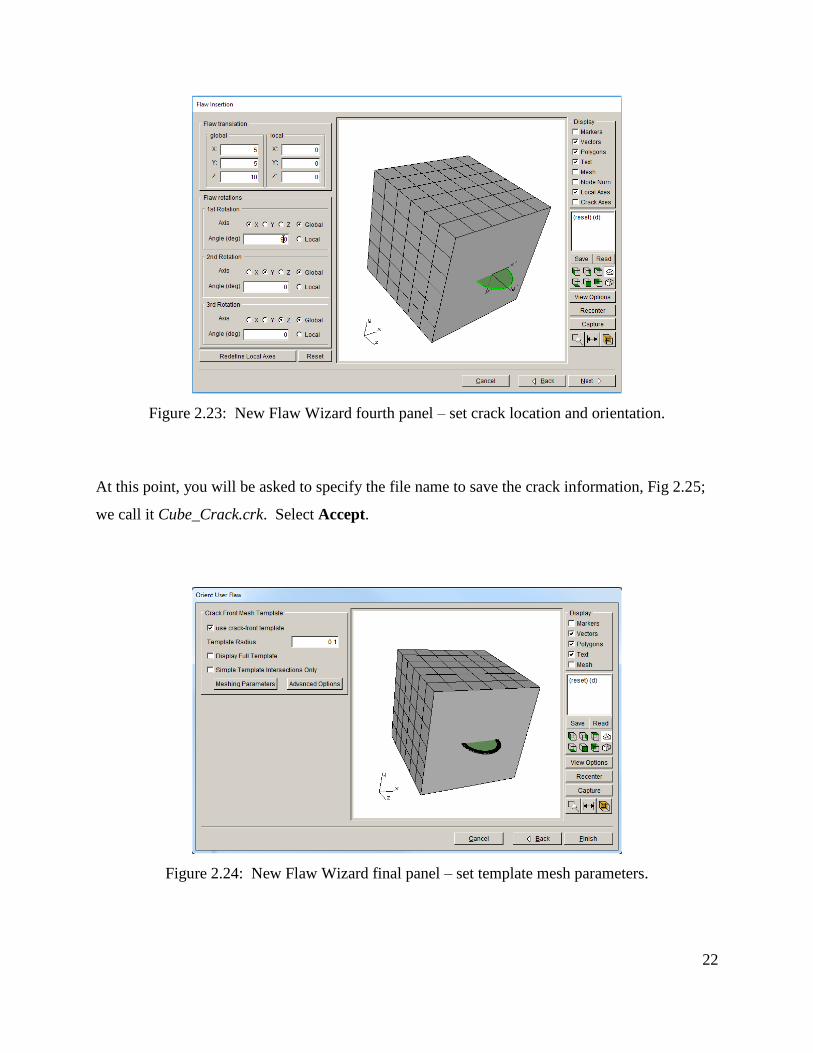
The fourth panel lets you set the crack location and orientation, Fig 2.23. We place the crack at
the center of the front face at coordinates (5,5,10) and rotate the crack 90 degrees about the
Global x-axis. Select Next.
The final panel allows you to set the crack front mesh template parameters, Fig 2.24; use the
defaults. In practice, the default template radius is based on the crack dimensions and might
need to be adjusted depending on the model and crack. Select Finish.
22
Figure 2.23: New Flaw Wizard fourth panel – set crack location and orientation.
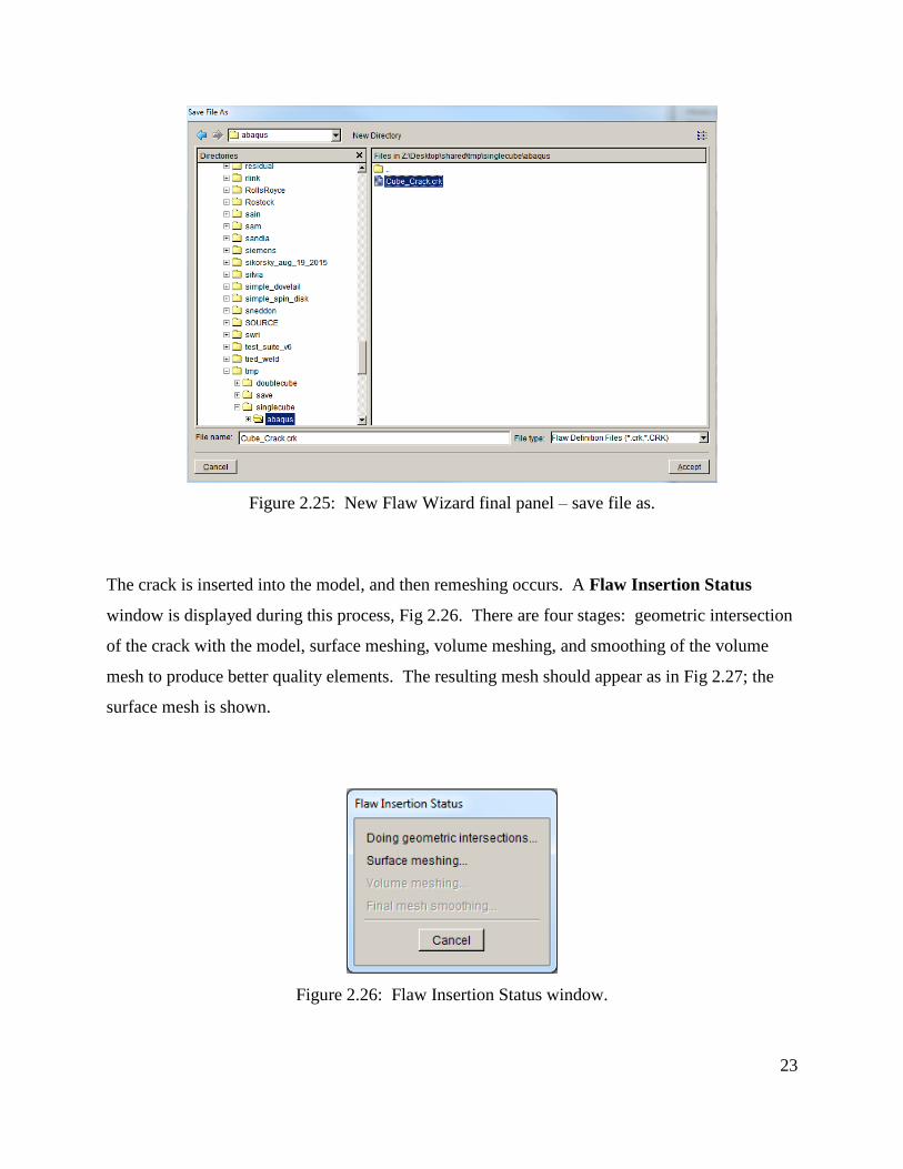
At this point, you will be asked to specify the file name to save the crack information, Fig 2.25;
we call it Cube_Crack.crk. Select Accept.
Figure 2.24: New Flaw Wizard final panel – set template mesh parameters.
23
Figure 2.25: New Flaw Wizard final panel – save file as.
The crack is inserted into the model, and then remeshing occurs. A Flaw Insertion Status
window is displayed during this process, Fig 2.26. There are four stages: geometric intersection
of the crack with the model, surface meshing, volume meshing, and smoothing of the volume
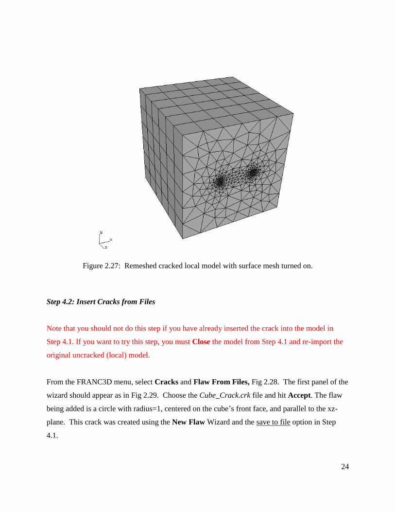
mesh to produce better quality elements. The resulting mesh should appear as in Fig 2.27; the
surface mesh is shown.
Figure 2.26: Flaw Insertion Status window.
24
Figure 2.27: Remeshed cracked local model with surface mesh turned on.
Step 4.2: Insert Cracks from Files
Note that you should not do this step if you have already inserted the crack into the model in
Step 4.1. If you want to try this step, you must Close the model from Step 4.1 and re-import the
original uncracked (local) model.
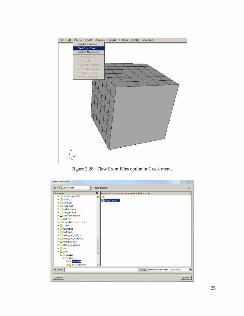
From the FRANC3D menu, select Cracks and Flaw From Files, Fig 2.28. The first panel of the
wizard should appear as in Fig 2.29. Choose the Cube_Crack.crk file and hit Accept. The flaw
being added is a circle with radius=1, centered on the cube’s front face, and parallel to the xz-
plane. This crack was created using the New Flaw Wizard and the save to file option in Step
4.1.
25
Figure 2.28: Flaw From Files option in Crack menu.
26
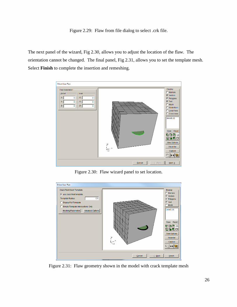
Figure 2.29: Flaw from file dialog to select .crk file.
The next panel of the wizard, Fig 2.30, allows you to adjust the location of the flaw. The
orientation cannot be changed. The final panel, Fig 2.31, allows you to set the template mesh.
Select Finish to complete the insertion and remeshing.
Figure 2.30: Flaw wizard panel to set location.
Figure 2.31: Flaw geometry shown in the model with crack template mesh

27
2.5 Step 5: Static Crack Analysis
Once the crack is inserted and remeshed, we must perform the stress analysis using ABAQUS,
which will provide the displacement results that are needed to compute stress intensity factors.
Typically, you should run a “static crack analysis” of the initial crack prior to running automated
crack growth; this allows you to verify that the crack model is consistent with the uncracked
model. (You might also try a smaller template to verify that the computed SIFs are accurate.)
Step 5.1: Select Static Crack Analysis
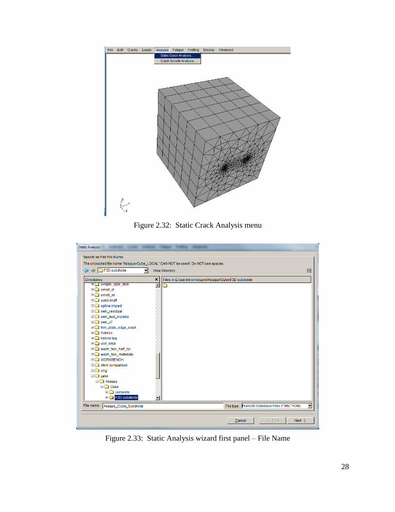
From the FRANC3D menu, select Analysis and Static Crack Analysis, Fig 2.32. The first
panel of the wizard, Fig 2.33, requests that you enter the file name for the FRANC3D data. We
call it Abaqus_Cube_Subdivide.fdb here; select Next once you enter the File Name.
Note that you cannot use the initial uncracked Abaqus_Cube.inp or Abaqus_Cube_LOCAL.inp
file names, because a new .inp file will be created and saved during the analysis, and the original
uncracked .inp files are reused for each step of crack growth.
28
Figure 2.32: Static Crack Analysis menu
Figure 2.33: Static Analysis wizard first panel – File Name
29
Step 5.2: Select FE Solver
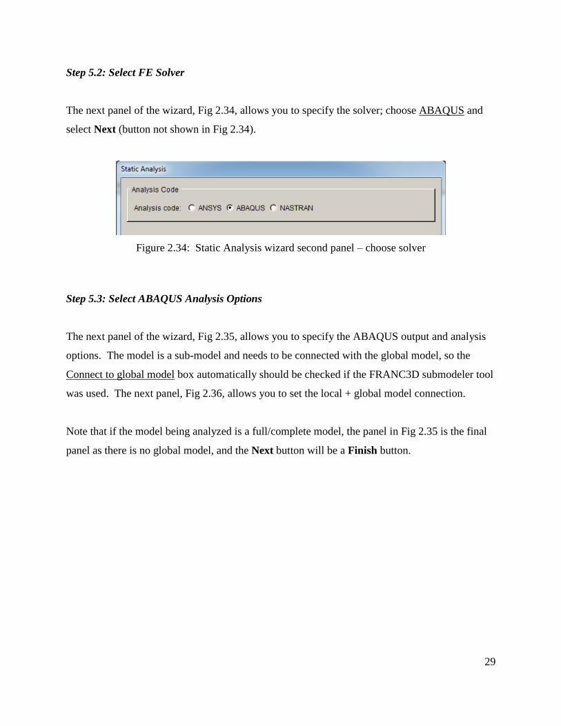
The next panel of the wizard, Fig 2.34, allows you to specify the solver; choose ABAQUS and
select Next (button not shown in Fig 2.34).
Figure 2.34: Static Analysis wizard second panel – choose solver
Step 5.3: Select ABAQUS Analysis Options
The next panel of the wizard, Fig 2.35, allows you to specify the ABAQUS output and analysis
options. The model is a sub-model and needs to be connected with the global model, so the
Connect to global model box automatically should be checked if the FRANC3D submodeler tool
was used. The next panel, Fig 2.36, allows you to set the local + global model connection.
Note that if the model being analyzed is a full/complete model, the panel in Fig 2.35 is the final
panel as there is no global model, and the Next button will be a Finish button.

30
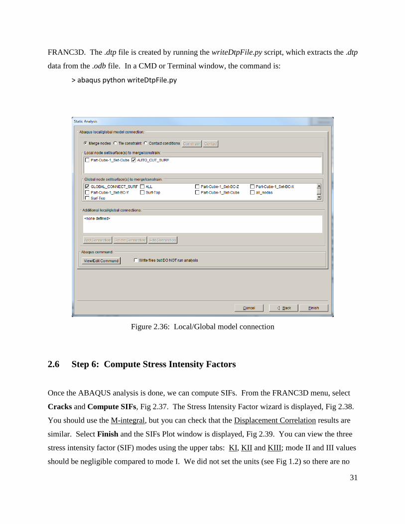
Figure 2.35: Static Analysis wizard third panel – ABAQUS output options
The panel in Fig 2.36 shows the options for joining the local and global models.
AUTO_CUT_SURF and GLOBAL_CONNECT_SURF are the node sets created by the
FRANC3D submodeling tool and should be selected automatically. Click Finish to start
ABAQUS running (in batch/background mode).
FRANC3D write files and then attempts to execute ABAQUS based on the ABAQUS
Executable information, Fig 2.35. You can monitor the FRANC3D CMD window and the
ABAQUS .dat and .msg file for errors or messages.
Choosing Write files but DO NOT run analysis in Fig 2.36 will create all the files without
running ABQUS, if the analysis needs to be run later or on a different computer. If you need to
run ABQUS on a different computer, you must bring the results file (.dtp) back to the working
folder, and then you can use the File and Read Results menu option to import the results into
31
FRANC3D. The .dtp file is created by running the writeDtpFile.py script, which extracts the .dtp
data from the .odb file. In a CMD or Terminal window, the command is:
> abaqus python writeDtpFile.py
Figure 2.36: Local/Global model connection
2.6 Step 6: Compute Stress Intensity Factors
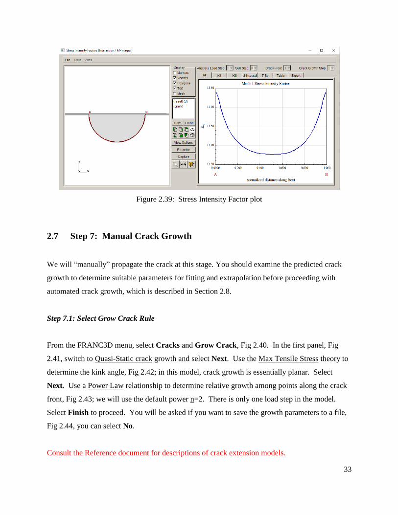
Once the ABAQUS analysis is done, we can compute SIFs. From the FRANC3D menu, select
Cracks and Compute SIFs, Fig 2.37. The Stress Intensity Factor wizard is displayed, Fig 2.38.
You should use the M-integral, but you can check that the Displacement Correlation results are
similar. Select Finish and the SIFs Plot window is displayed, Fig 2.39. You can view the three
stress intensity factor (SIF) modes using the upper tabs: KI, KII and KIII; mode II and III values
should be negligible compared to mode I. We did not set the units (see Fig 1.2) so there are no

32
units displayed on the SIF plot. You can set the FEM units using the Edit menu and recompute
SIFs to display with units.
Figure 2.37: Compute SIF’s selected from the Cracks menu
Figure 2.38: Compute SIF options
33
Figure 2.39: Stress Intensity Factor plot
2.7 Step 7: Manual Crack Growth
We will “manually” propagate the crack at this stage. You should examine the predicted crack
growth to determine suitable parameters for fitting and extrapolation before proceeding with
automated crack growth, which is described in Section 2.8.
Step 7.1: Select Grow Crack Rule
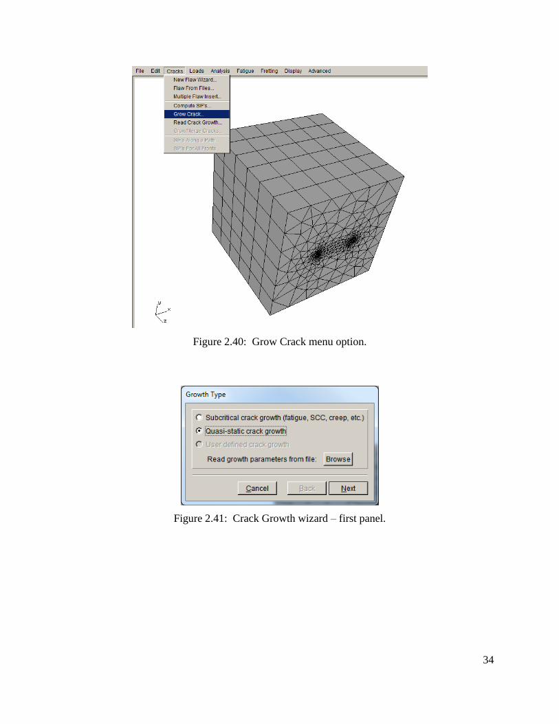
From the FRANC3D menu, select Cracks and Grow Crack, Fig 2.40. In the first panel, Fig
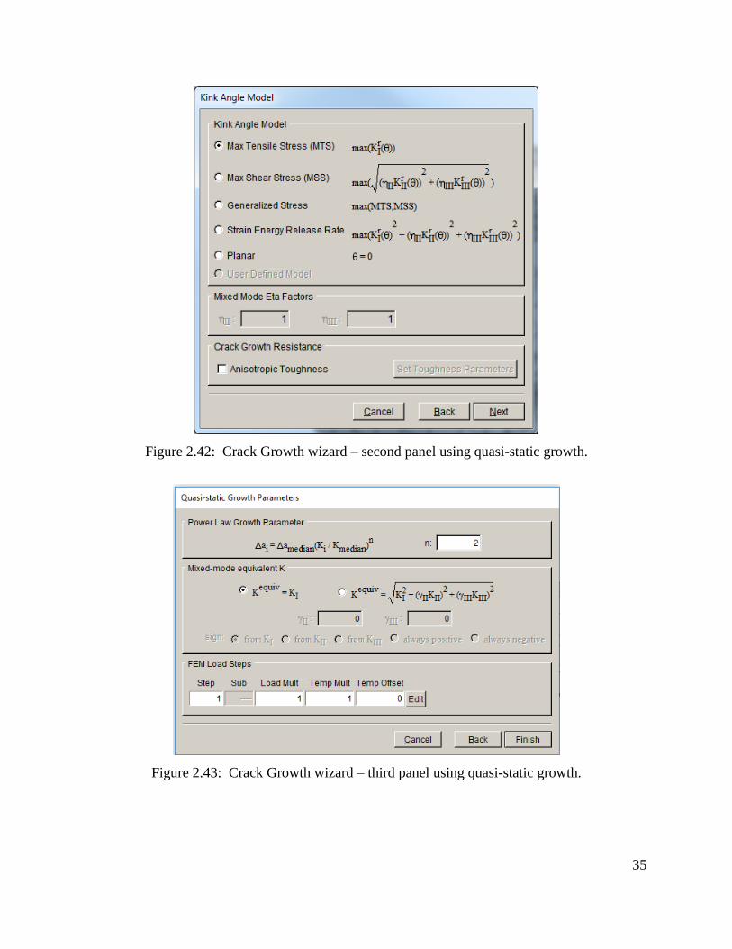
2.41, switch to Quasi-Static crack growth and select Next. Use the Max Tensile Stress theory to
determine the kink angle, Fig 2.42; in this model, crack growth is essentially planar. Select
Next. Use a Power Law relationship to determine relative growth among points along the crack
front, Fig 2.43; we will use the default power n=2. There is only one load step in the model.
Select Finish to proceed. You will be asked if you want to save the growth parameters to a file,
Fig 2.44, you can select No.
Consult the Reference document for descriptions of crack extension models.
34
Figure 2.40: Grow Crack menu option.
Figure 2.41: Crack Growth wizard – first panel.
35
Figure 2.42: Crack Growth wizard – second panel using quasi-static growth.
Figure 2.43: Crack Growth wizard – third panel using quasi-static growth.
36
Figure 2.44: Save growth parameters dialog.
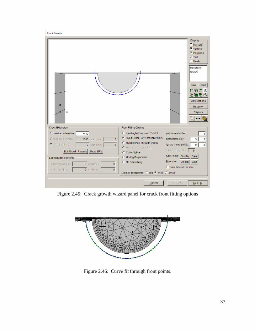
Step 7.2: Specify Fitting and Extrapolation
The next panel, Fig 2.45 allows you to specify the crack front point fitting parameters. You can
double click on the (crack) view to see the crack surface; this should be the default view. The
median extension is set to 0.15; this value generally is set automatically based on the initial
template radius so your value might be different. We change it to 0.12 and turn on Mesh and
Markers (top right of Fig 2.45). The green boxes are the computed points and the blue line is the
curve-fit, Fig 2.46.
A Fixed Order Polynomial fit with order set to 3 and extrapolation set to 3% at both ends of the
crack front is the default; the fitting parameters might need to be adjusted as the crack grows. A
4th order polynomial might provide a slightly better fit in this case; the guidelines for curve-
fitting are to use the simplest fit that is reasonable. We stick with the default 3rd order
polynomial; select Next to proceed.
Note that the fitted (blue) curve through the predicted new front points (green) must be
extrapolated so that both ends fall outside of the model, but it should not be extrapolated too
much.
The median extension must be enough to provide finite space between the current and new fronts
along the entire front to define new crack geometry.
37
Figure 2.45: Crack growth wizard panel for crack front fitting options
Figure 2.46: Curve fit through front points.
38
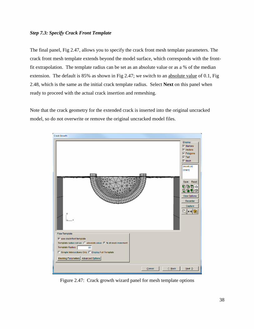
Step 7.3: Specify Crack Front Template
The final panel, Fig 2.47, allows you to specify the crack front mesh template parameters. The
crack front mesh template extends beyond the model surface, which corresponds with the front-
fit extrapolation. The template radius can be set as an absolute value or as a % of the median
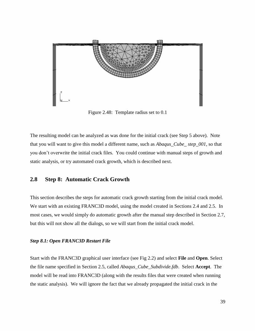
extension. The default is 85% as shown in Fig 2.47; we switch to an absolute value of 0.1, Fig
2.48, which is the same as the initial crack template radius. Select Next on this panel when
ready to proceed with the actual crack insertion and remeshing.
Note that the crack geometry for the extended crack is inserted into the original uncracked
model, so do not overwrite or remove the original uncracked model files.
Figure 2.47: Crack growth wizard panel for mesh template options
39
Figure 2.48: Template radius set to 0.1
The resulting model can be analyzed as was done for the initial crack (see Step 5 above). Note
that you will want to give this model a different name, such as Abaqus_Cube_ step_001, so that
you don’t overwrite the initial crack files. You could continue with manual steps of growth and
static analysis, or try automated crack growth, which is described next.
2.8 Step 8: Automatic Crack Growth
This section describes the steps for automatic crack growth starting from the initial crack model.
We start with an existing FRANC3D model, using the model created in Sections 2.4 and 2.5. In
most cases, we would simply do automatic growth after the manual step described in Section 2.7,
but this will not show all the dialogs, so we will start from the initial crack model.
Step 8.1: Open FRANC3D Restart File
Start with the FRANC3D graphical user interface (see Fig 2.2) and select File and Open. Select
the file name specified in Section 2.5, called Abaqus_Cube_Subdivide.fdb. Select Accept. The
model will be read into FRANC3D (along with the results files that were created when running
the static analysis). We will ignore the fact that we already propagated the initial crack in the
40
previous step (but we will use the settings), and proceed with setting up the automatic crack
growth analysis.
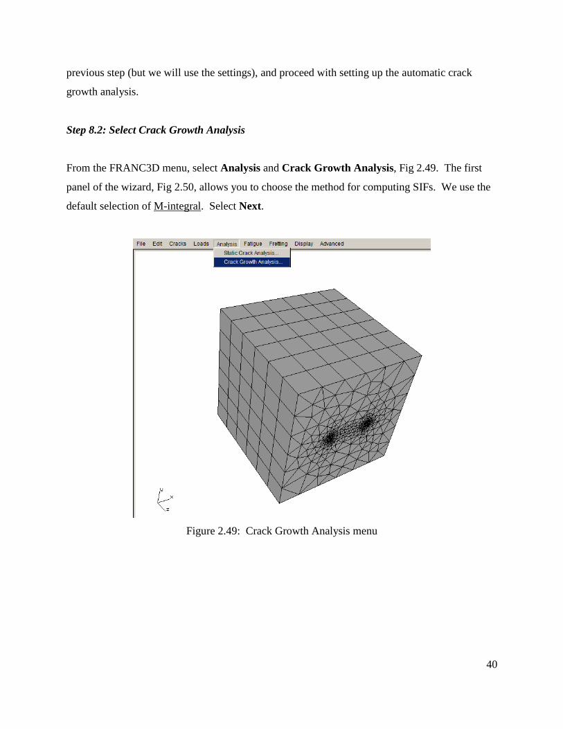
Step 8.2: Select Crack Growth Analysis
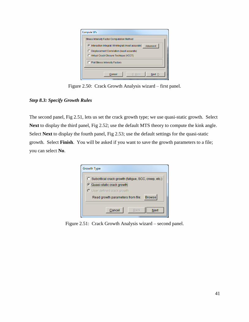
From the FRANC3D menu, select Analysis and Crack Growth Analysis, Fig 2.49. The first
panel of the wizard, Fig 2.50, allows you to choose the method for computing SIFs. We use the
default selection of M-integral. Select Next.
Figure 2.49: Crack Growth Analysis menu
41
Figure 2.50: Crack Growth Analysis wizard – first panel.
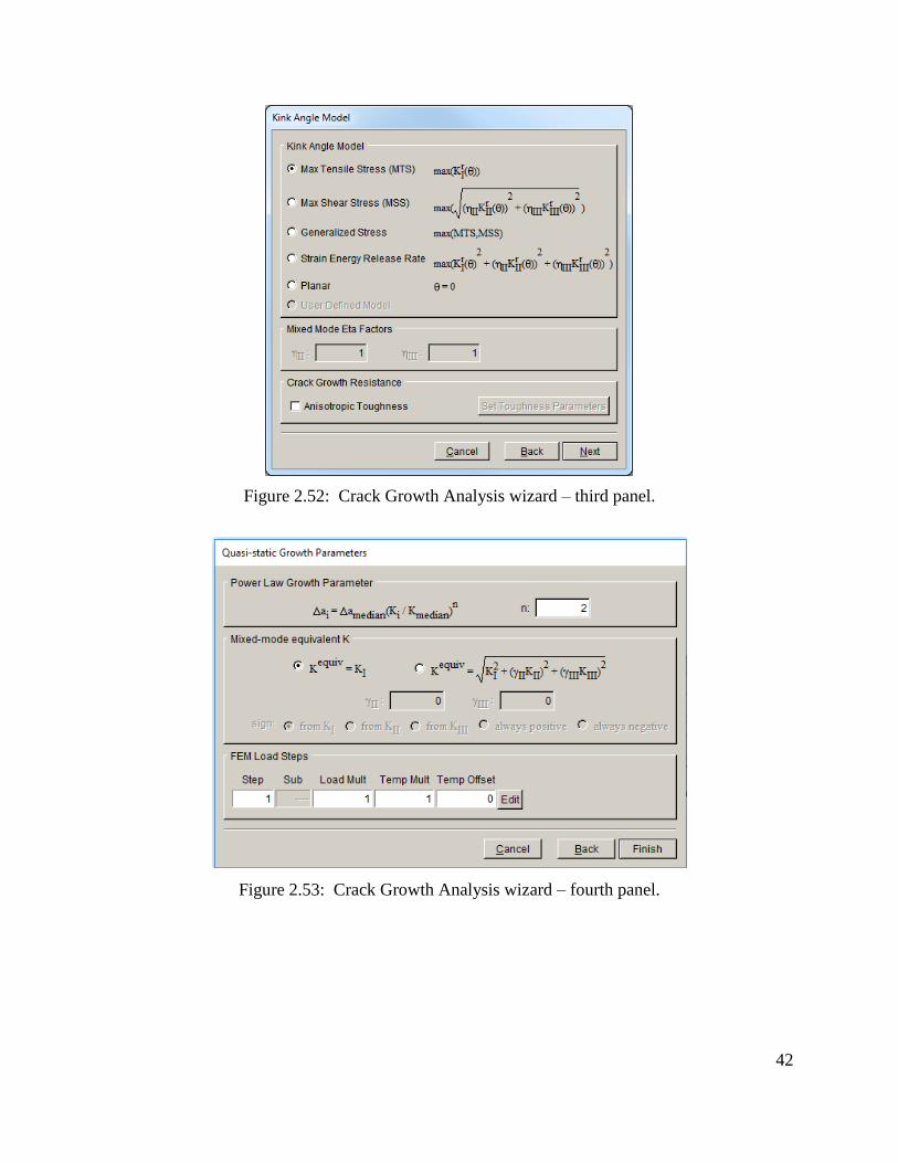
Step 8.3: Specify Growth Rules
The second panel, Fig 2.51, lets us set the crack growth type; we use quasi-static growth. Select
Next to display the third panel, Fig 2.52; use the default MTS theory to compute the kink angle.
Select Next to display the fourth panel, Fig 2.53; use the default settings for the quasi-static
growth. Select Finish. You will be asked if you want to save the growth parameters to a file;
you can select No.
Figure 2.51: Crack Growth Analysis wizard – second panel.
42
Figure 2.52: Crack Growth Analysis wizard – third panel.
Figure 2.53: Crack Growth Analysis wizard – fourth panel.
43
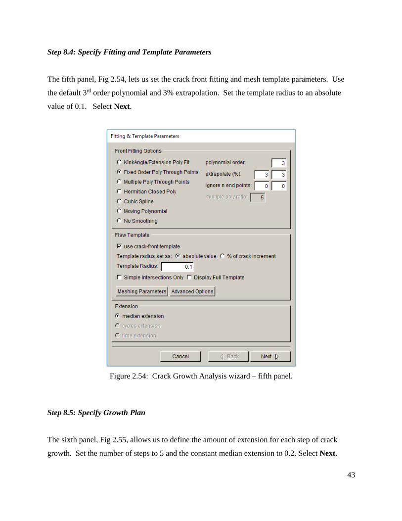
Step 8.4: Specify Fitting and Template Parameters
The fifth panel, Fig 2.54, lets us set the crack front fitting and mesh template parameters. Use
the default 3rd order polynomial and 3% extrapolation. Set the template radius to an absolute
value of 0.1. Select Next.
Figure 2.54: Crack Growth Analysis wizard – fifth panel.
Step 8.5: Specify Growth Plan
The sixth panel, Fig 2.55, allows us to define the amount of extension for each step of crack
growth. Set the number of steps to 5 and the constant median extension to 0.2. Select Next.

44
Note that we are taking a relatively large crack growth step here; this is to limit the number of
steps and time for this tutorial. Large steps can sometimes lead to issues with oscillations in the
shape of the crack fronts (see Section 9.5 of the User’s Guide).
Figure 2.55: Crack Growth Analysis wizard – sixth panel.
Step 8.6: Specify Analysis Code
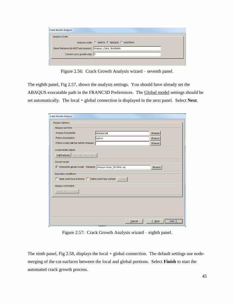
The seventh panel of the wizard, Fig 2.56, lets us choose the analysis code; we use ABAQUS.
The current crack growth step defaults to 0 – representing the initial crack. If we had “manually”
propagated the crack first, we would set this to 1. FRANC3D will extend the initial crack based
on the growth rule defined in the previous panels, and then name the resulting set of files as
Abaqus_Cube_Subdivide_STEP_001.*. Subsequent file names have the step number
incremented as the automatic analysis proceeds. Select Next (button not shown).
45
Figure 2.56: Crack Growth Analysis wizard – seventh panel.
The eighth panel, Fig 2.57, shows the analysis settings. You should have already set the
ABAQUS executable path in the FRANC3D Preferences. The Global model settings should be
set automatically. The local + global connection is displayed in the next panel. Select Next.
Figure 2.57: Crack Growth Analysis wizard – eighth panel.
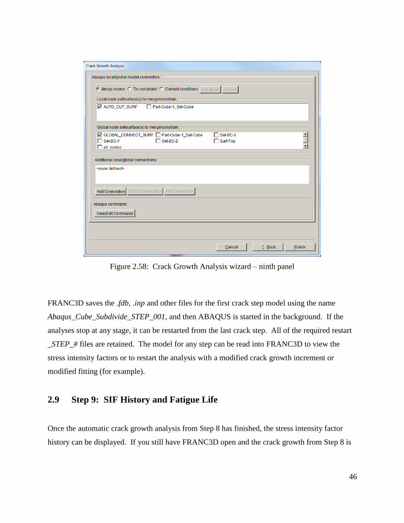
The ninth panel, Fig 2.58, displays the local + global connection. The default settings use node-
merging of the cut-surfaces between the local and global portions. Select Finish to start the
automated crack growth process.
46
Figure 2.58: Crack Growth Analysis wizard – ninth panel
FRANC3D saves the .fdb, .inp and other files for the first crack step model using the name
Abaqus_Cube_Subdivide_STEP_001, and then ABAQUS is started in the background. If the
analyses stop at any stage, it can be restarted from the last crack step. All of the required restart
_STEP_# files are retained. The model for any step can be read into FRANC3D to view the
stress intensity factors or to restart the analysis with a modified crack growth increment or
modified fitting (for example).
2.9 Step 9: SIF History and Fatigue Life
Once the automatic crack growth analysis from Step 8 has finished, the stress intensity factor
history can be displayed. If you still have FRANC3D open and the crack growth from Step 8 is
47
done, you can proceed with Step 9.1. Otherwise, you can restart FRANC3D and read in the .fdb
file for the last step, using the File and Open menu option.
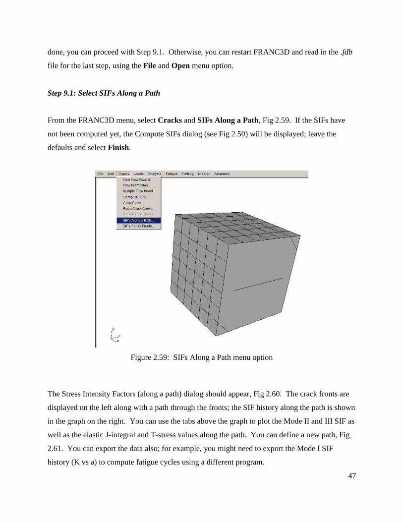
Step 9.1: Select SIFs Along a Path
From the FRANC3D menu, select Cracks and SIFs Along a Path, Fig 2.59. If the SIFs have
not been computed yet, the Compute SIFs dialog (see Fig 2.50) will be displayed; leave the
defaults and select Finish.
Figure 2.59: SIFs Along a Path menu option
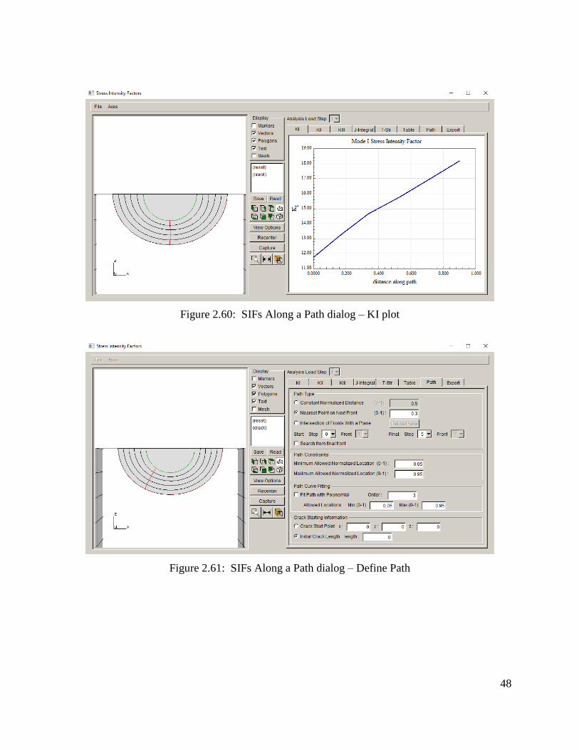
The Stress Intensity Factors (along a path) dialog should appear, Fig 2.60. The crack fronts are
displayed on the left along with a path through the fronts; the SIF history along the path is shown
in the graph on the right. You can use the tabs above the graph to plot the Mode II and III SIF as
well as the elastic J-integral and T-stress values along the path. You can define a new path, Fig
2.61. You can export the data also; for example, you might need to export the Mode I SIF
history (K vs a) to compute fatigue cycles using a different program.
48
Figure 2.60: SIFs Along a Path dialog – KI plot
Figure 2.61: SIFs Along a Path dialog – Define Path
49
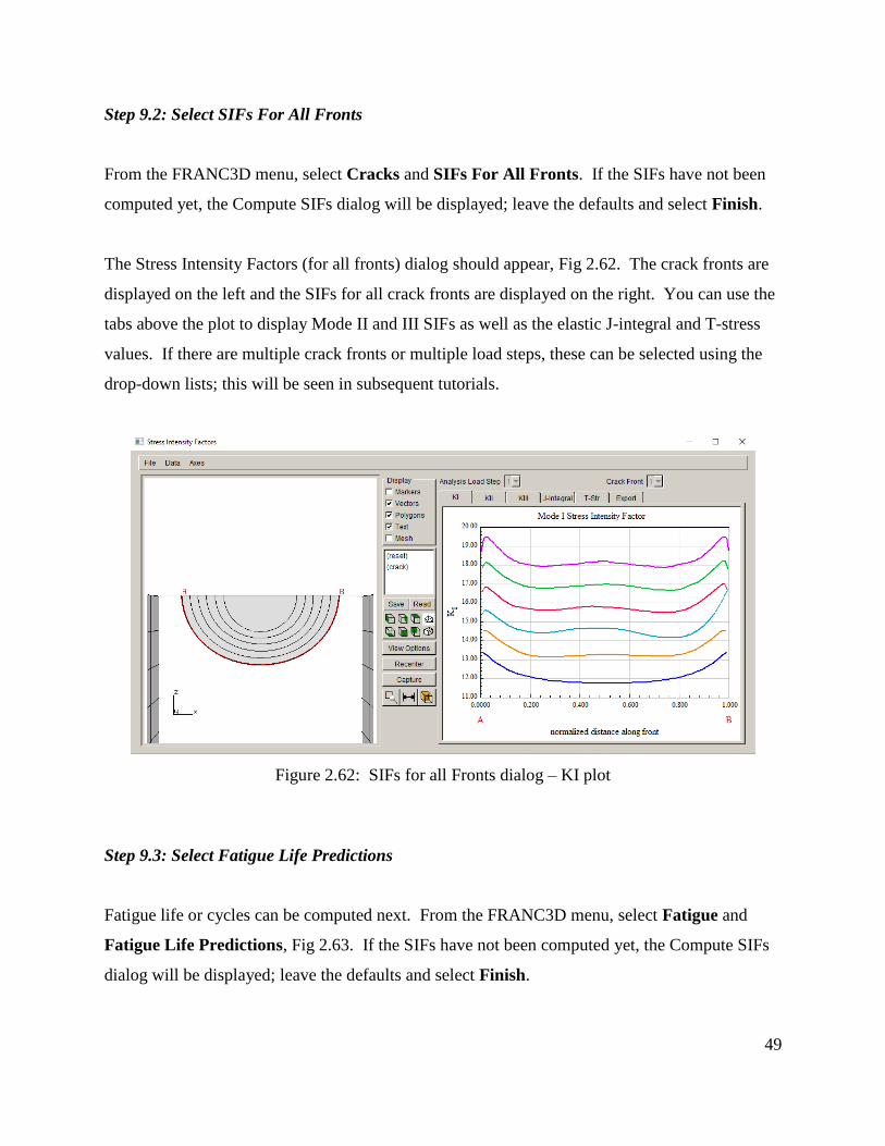
Step 9.2: Select SIFs For All Fronts
From the FRANC3D menu, select Cracks and SIFs For All Fronts. If the SIFs have not been
computed yet, the Compute SIFs dialog will be displayed; leave the defaults and select Finish.
The Stress Intensity Factors (for all fronts) dialog should appear, Fig 2.62. The crack fronts are
displayed on the left and the SIFs for all crack fronts are displayed on the right. You can use the
tabs above the plot to display Mode II and III SIFs as well as the elastic J-integral and T-stress
values. If there are multiple crack fronts or multiple load steps, these can be selected using the
drop-down lists; this will be seen in subsequent tutorials.
Figure 2.62: SIFs for all Fronts dialog – KI plot
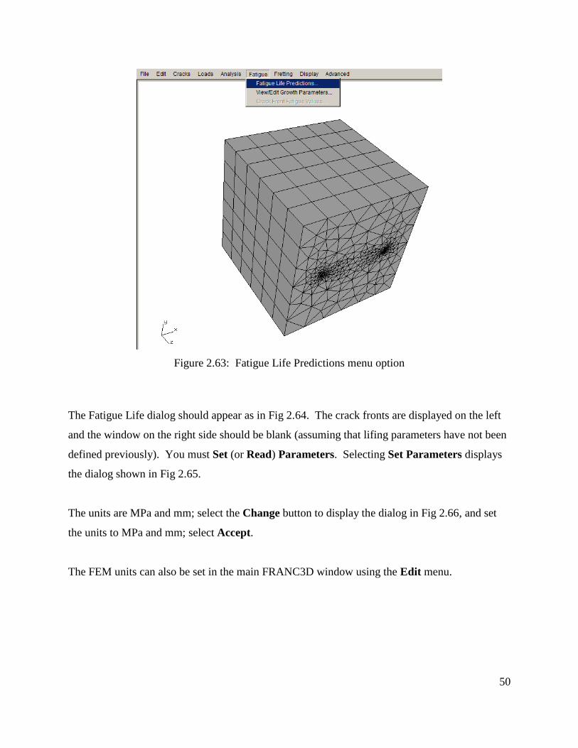
Step 9.3: Select Fatigue Life Predictions
Fatigue life or cycles can be computed next. From the FRANC3D menu, select Fatigue and
Fatigue Life Predictions, Fig 2.63. If the SIFs have not been computed yet, the Compute SIFs
dialog will be displayed; leave the defaults and select Finish.
50
Figure 2.63: Fatigue Life Predictions menu option
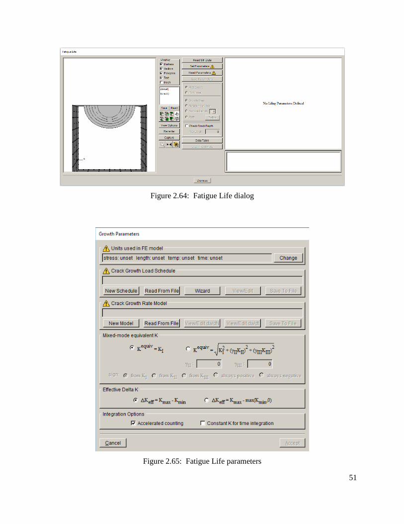
The Fatigue Life dialog should appear as in Fig 2.64. The crack fronts are displayed on the left
and the window on the right side should be blank (assuming that lifing parameters have not been
defined previously). You must Set (or Read) Parameters. Selecting Set Parameters displays
the dialog shown in Fig 2.65.
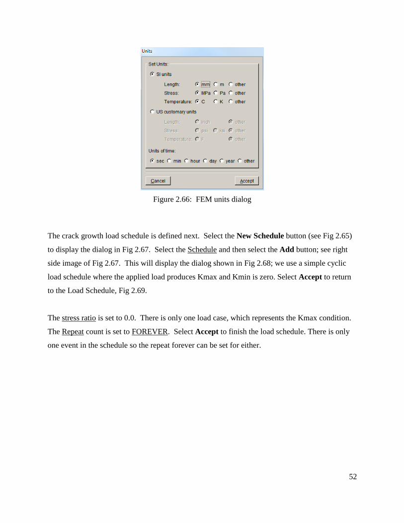
The units are MPa and mm; select the Change button to display the dialog in Fig 2.66, and set
the units to MPa and mm; select Accept.
The FEM units can also be set in the main FRANC3D window using the Edit menu.
51
Figure 2.64: Fatigue Life dialog
Figure 2.65: Fatigue Life parameters
52
Figure 2.66: FEM units dialog
The crack growth load schedule is defined next. Select the New Schedule button (see Fig 2.65)
to display the dialog in Fig 2.67. Select the Schedule and then select the Add button; see right
side image of Fig 2.67. This will display the dialog shown in Fig 2.68; we use a simple cyclic
load schedule where the applied load produces Kmax and Kmin is zero. Select Accept to return
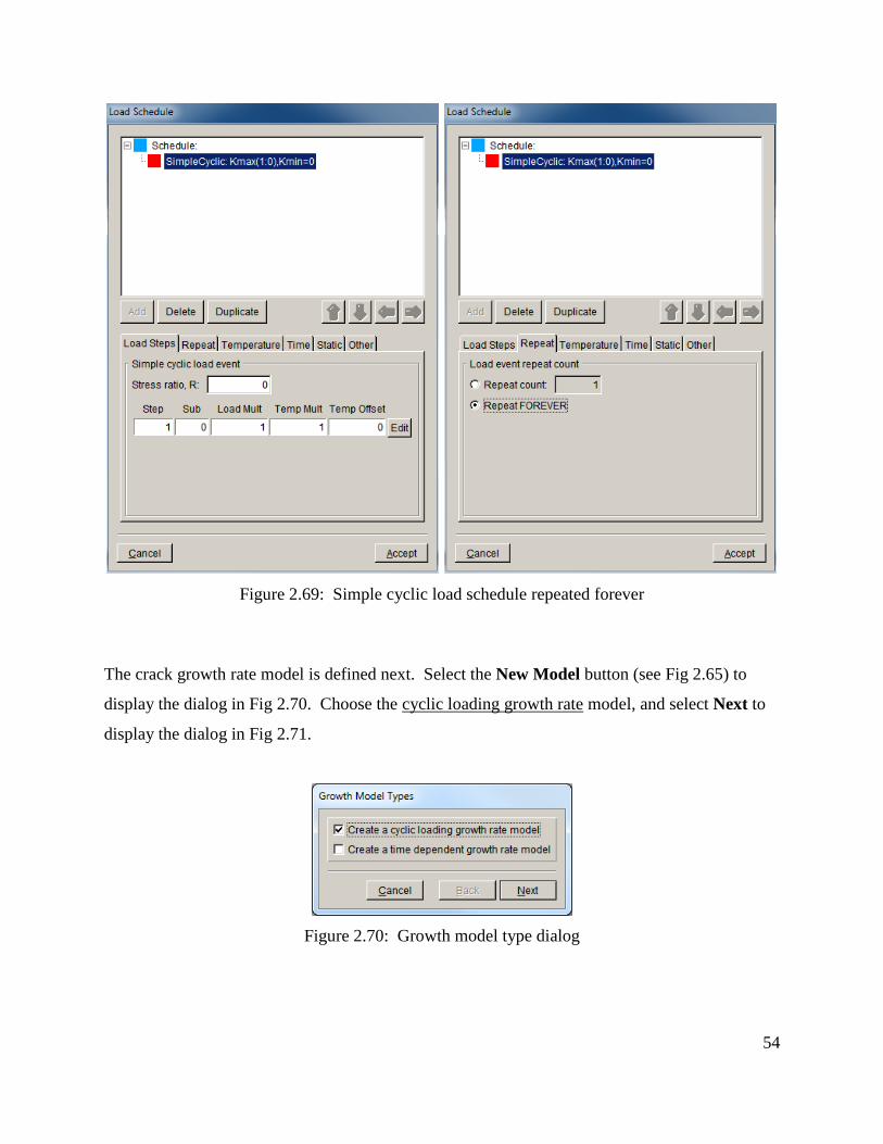
to the Load Schedule, Fig 2.69.
The stress ratio is set to 0.0. There is only one load case, which represents the Kmax condition.
The Repeat count is set to FOREVER. Select Accept to finish the load schedule. There is only
one event in the schedule so the repeat forever can be set for either.

53
Figure 2.67: New Load Schedule dialog
Figure 2.68: Event type dialog
54
Figure 2.69: Simple cyclic load schedule repeated forever
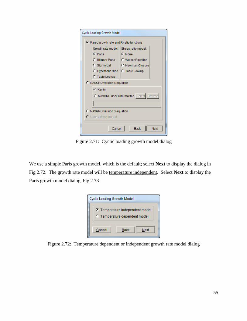
The crack growth rate model is defined next. Select the New Model button (see Fig 2.65) to
display the dialog in Fig 2.70. Choose the cyclic loading growth rate model, and select Next to
display the dialog in Fig 2.71.
Figure 2.70: Growth model type dialog
55
Figure 2.71: Cyclic loading growth model dialog
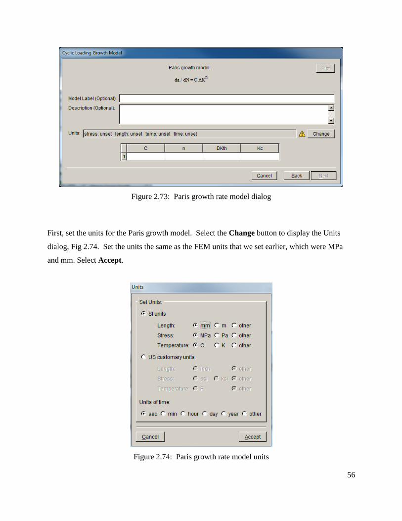
We use a simple Paris growth model, which is the default; select Next to display the dialog in
Fig 2.72. The growth rate model will be temperature independent. Select Next to display the
Paris growth model dialog, Fig 2.73.
Figure 2.72: Temperature dependent or independent growth rate model dialog
56
Figure 2.73: Paris growth rate model dialog
First, set the units for the Paris growth model. Select the Change button to display the Units
dialog, Fig 2.74. Set the units the same as the FEM units that we set earlier, which were MPa
and mm. Select Accept.
Figure 2.74: Paris growth rate model units

57
In the Paris growth model dialog, click on the fields for C, n, DKth and Kc and enter the
appropriate values, Fig 2.75. Select Next to return the main dialog (see Fig 2.65). The other
options are left at their default values; select Accept to return to the Fatigue Life dialog, Fig
2.76.
Figure 2.75: Paris growth rate model values
Figure 2.76: Fatigue life showing Cycles vs Crack Growth Step
58
Note that the Paris exponent ‘n’ is set to 3 whereas we used n=2 for the quasi-static growth. In
practice, you can use the fatigue model and material data to compute growth so that it is
consistent with the fatigue life computations done here. However, it is not strictly necessary, and
it might work better to use a lower exponent to predict increments of growth.
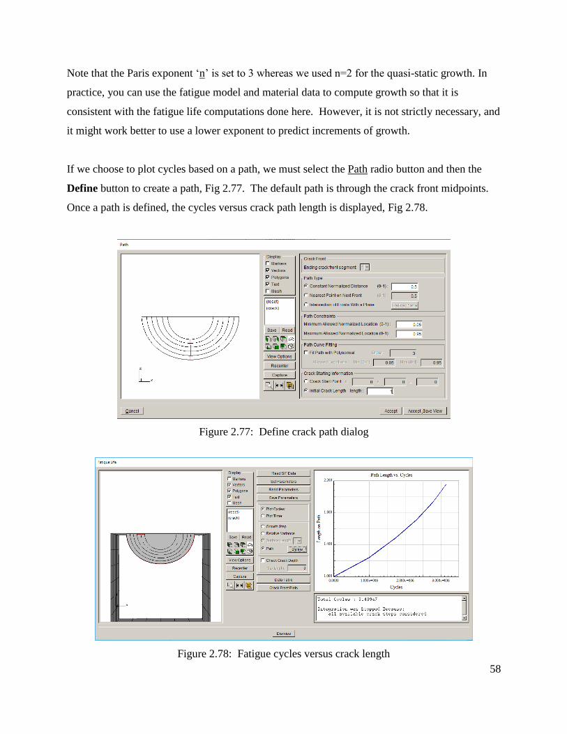
If we choose to plot cycles based on a path, we must select the Path radio button and then the
Define button to create a path, Fig 2.77. The default path is through the crack front midpoints.
Once a path is defined, the cycles versus crack path length is displayed, Fig 2.78.
Figure 2.77: Define crack path dialog
Figure 2.78: Fatigue cycles versus crack length
59
2.10 Step 10: Resume Growth with Larger Submodel
We used a local submodel for this crack growth simulation. If the crack growth exceeds the
boundary of the local submodel, a larger submodel can be selected and crack growth can be
continued without having to restart the simulation from the beginning. In this step, we describe
the process of extracting the current crack geometry and inserting this into a larger portion of the
model to resume crack growth.
Step 10.1: Extract and Save Crack Geometry
The crack geometry information for each step of crack growth is saved in the FRANC3D restart
(.fdb) file. The data appears in this block:
FLAWSURF ( VERSION: 5 NUM_SURFS: 763 SURF: 0 263 264 356 6.83559456365193 5.00380971299962 9.72712346638146 … … 4.73891556707121 5.00420103803897 8.3468309877949 )
This data can be copied from the .fdb file and saved to a .crk file, using any text editor.
We open the Abaqus_Cube_subdivide_STEP_005.fdb file, copy the FLAWSURF data, and save
it to a .crk file, called Abaqus_Cube _step_5.crk.
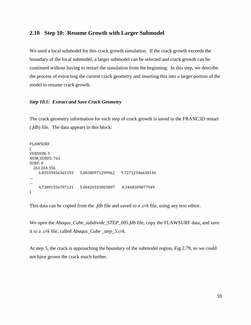
At step 5, the crack is approaching the boundary of the submodel region, Fig 2.79, so we could
not have grown the crack much further.
60
Figure 2.79: Crack step 5 in local submodel.
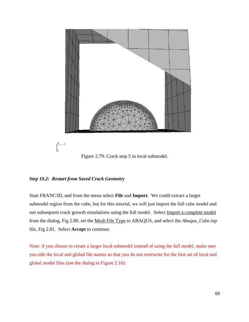
Step 10.2: Restart from Saved Crack Geometry
Start FRANC3D, and from the menu select File and Import. We could extract a larger
submodel region from the cube, but for this tutorial, we will just import the full cube model and
run subsequent crack growth simulations using the full model. Select Import a complete model
from the dialog, Fig 2.80, set the Mesh File Type to ABAQUS, and select the Abaqus_Cube.inp
file, Fig 2.81. Select Accept to continue.
Note: if you choose to create a larger local submodel instead of using the full model, make sure
you edit the local and global file names so that you do not overwrite for the first set of local and
global model files (see the dialog in Figure 2.16).

61
Figure 2.80: FRANC3D model import dialog.
Figure 2.81: FRANC3D mesh import file selector.
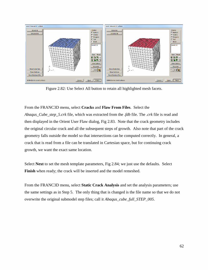
Use the Select All button in the next dialog, Fig 2.82, to retain all the mesh facets where
boundary conditions are applied. Select FINISH when ready; the model will be imported and
displayed in the FRANC3D main window.
62
Figure 2.82: Use Select All button to retain all highlighted mesh facets.
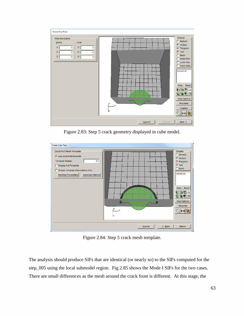
From the FRANC3D menu, select Cracks and Flaw From Files. Select the
Abaqus_Cube_step_5.crk file, which was extracted from the .fdb file. The .crk file is read and
then displayed in the Orient User Flaw dialog, Fig 2.83. Note that the crack geometry includes
the original circular crack and all the subsequent steps of growth. Also note that part of the crack
geometry falls outside the model so that intersections can be computed correctly. In general, a
crack that is read from a file can be translated in Cartesian space, but for continuing crack
growth, we want the exact same location.
Select Next to set the mesh template parameters, Fig 2.84; we just use the defaults. Select
Finish when ready; the crack will be inserted and the model remeshed.
From the FRANC3D menu, select Static Crack Analysis and set the analysis parameters; use
the same settings as in Step 5. The only thing that is changed is the file name so that we do not
overwrite the original submodel step files; call it Abaqus_cube_full_STEP_005.
63
Figure 2.83: Step 5 crack geometry displayed in cube model.
Figure 2.84: Step 5 crack mesh template.
The analysis should produce SIFs that are identical (or nearly so) to the SIFs computed for the
step_005 using the local submodel region. Fig 2.85 shows the Mode I SIFs for the two cases.
There are small differences as the mesh around the crack front is different. At this stage, the
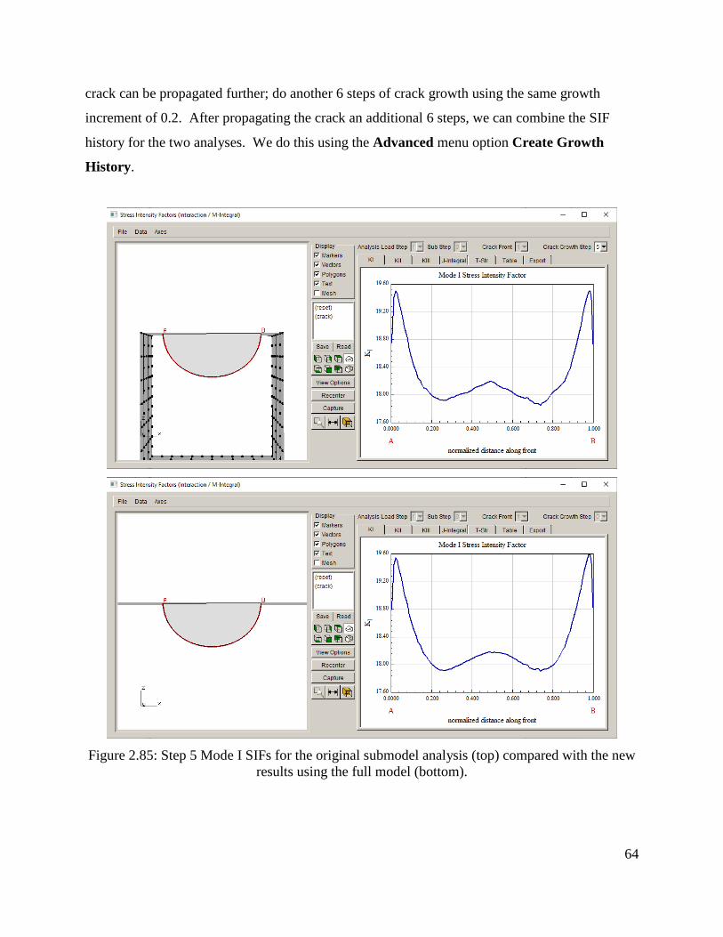
64
crack can be propagated further; do another 6 steps of crack growth using the same growth
increment of 0.2. After propagating the crack an additional 6 steps, we can combine the SIF
history for the two analyses. We do this using the Advanced menu option Create Growth
History.
Figure 2.85: Step 5 Mode I SIFs for the original submodel analysis (top) compared with the new
results using the full model (bottom).
65
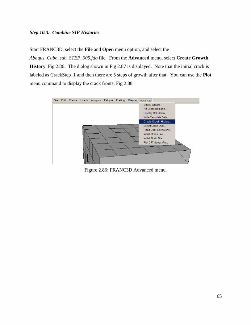
Step 10.3: Combine SIF Histories
Start FRANC3D, select the File and Open menu option, and select the
Abaqus_Cube_sub_STEP_005.fdb file. From the Advanced menu, select Create Growth
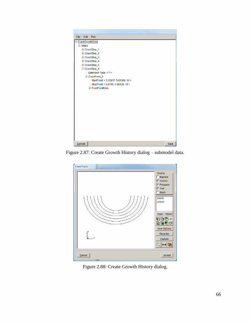
History, Fig 2.86. The dialog shown in Fig 2.87 is displayed. Note that the initial crack is
labeled as CrackStep_1 and then there are 5 steps of growth after that. You can use the Plot
menu command to display the crack fronts, Fig 2.88.
Figure 2.86: FRANC3D Advanced menu.
66
Figure 2.87: Create Growth History dialog – submodel data.
Figure 2.88: Create Growth History dialog.
67
Using the File menu in the Create Growth History dialog, select Save History, Fig 2.89, and
save the SIF history to a .fcg file, called Abaqus_Cube_sub_steps.fcg here. Close the dialog
using the Cancel button, and then close the model in FRANC3D using the main File menu Close
option.
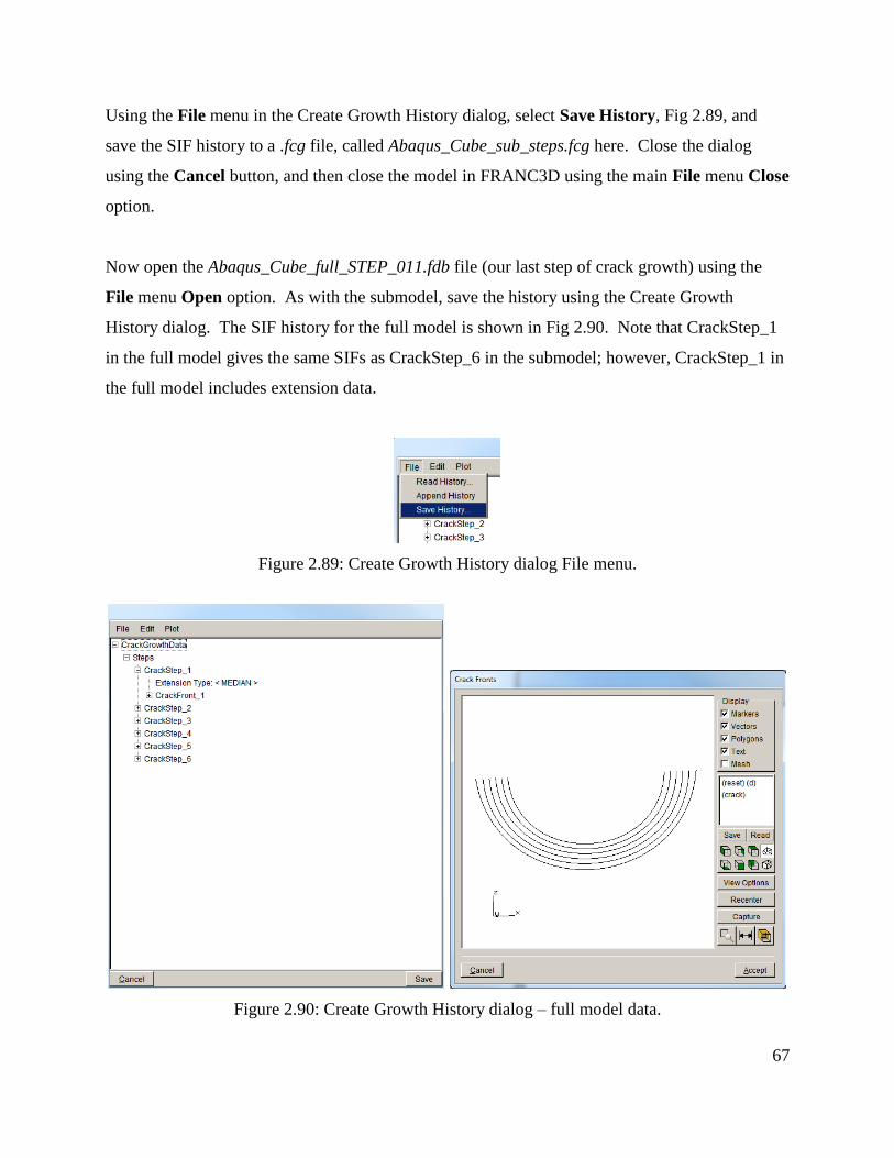
Now open the Abaqus_Cube_full_STEP_011.fdb file (our last step of crack growth) using the
File menu Open option. As with the submodel, save the history using the Create Growth
History dialog. The SIF history for the full model is shown in Fig 2.90. Note that CrackStep_1
in the full model gives the same SIFs as CrackStep_6 in the submodel; however, CrackStep_1 in
the full model includes extension data.
Figure 2.89: Create Growth History dialog File menu.
Figure 2.90: Create Growth History dialog – full model data.

68
Save the full model SIF history to a .fcg file, called Abaqus_Cube_full_steps.fcg here. Close the
Create Growth History dialog and close the model. This leaves the FRANC3D main model
window empty. Select the Advanced and Create Growth History menu option to display the
dialog. It does not have any CrackGrowthData.
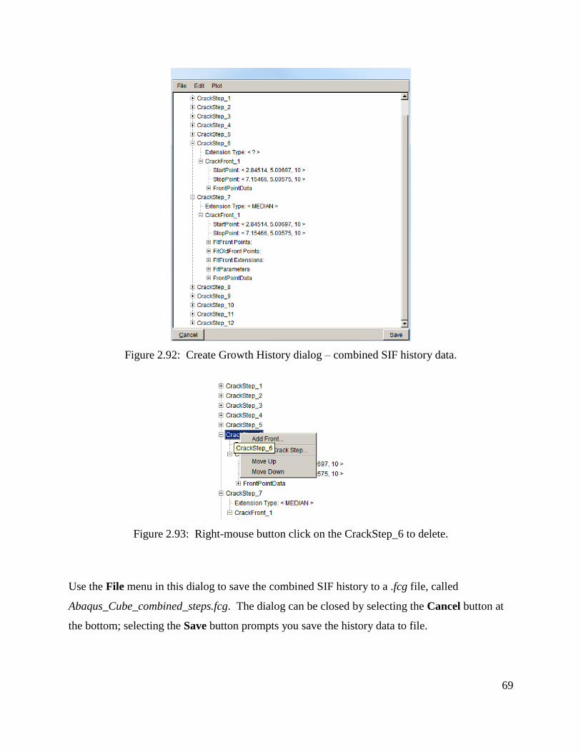
Use the File menu in the Create Growth History dialog and select Read History, Fig 2.91.
Select the Abaqus_Cube_sub_steps.fcg file. Then using the same menu, select Append History
and select the Abaqus_Cube_full_steps.fcg file. Note that there will be 12 steps of crack data at
this stage, Fig 2.92. We need to delete CrackStep_6 from the Submodel data as it does not
include extension data. We highlight CrackStep_6, Fig 2.93, and then right-click the mouse to
display the submenu, Fig 2.93. Select Delete Crack Step and it will be removed, leaving 11
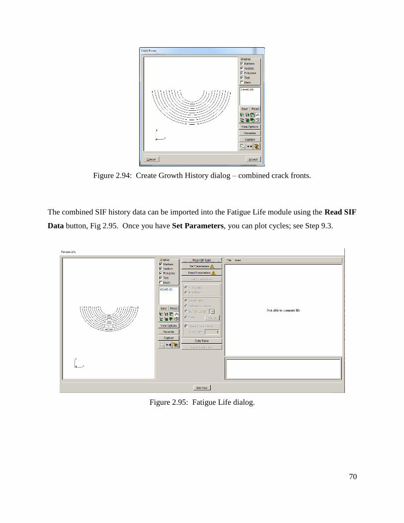
crack steps. You can plot the combined fronts, Fig 2.94.
Figure 2.91: Create Growth History dialog – File menu.
69
Figure 2.92: Create Growth History dialog – combined SIF history data.
Figure 2.93: Right-mouse button click on the CrackStep_6 to delete.
Use the File menu in this dialog to save the combined SIF history to a .fcg file, called
Abaqus_Cube_combined_steps.fcg. The dialog can be closed by selecting the Cancel button at
the bottom; selecting the Save button prompts you save the history data to file.
70
Figure 2.94: Create Growth History dialog – combined crack fronts.
The combined SIF history data can be imported into the Fatigue Life module using the Read SIF
Data button, Fig 2.95. Once you have Set Parameters, you can plot cycles; see Step 9.3.
Figure 2.95: Fatigue Life dialog.

71
Appendix A: ABAQUS local model defined between *Tie
constraints
This example describes how one can use an already-divided ABAQUS model, where the local
portion is tied to the global portion using *TIE constraints. Figure A1 shows the complete model
of a simple hinge. The local portion that will be extracted and imported into FRANC3D is
contained between the two *TIE surfaces. This complete model can be copied to a local and
global model and the appropriate portions of the model saved as separate .inp files. In this
example, the files are named: hinge-global.inp and hinge-local.inp. Once these two files are
saved, we can proceed to FRANC3D.
Figure A1. ABAQUS hinge model; local portion is contained between two *TIE surfaces.

72
From the FRANC3D File menu, select Import. The first dialog is shown in Figure A2; select the
Import an already divided model option and click Next. The second dialog, Figure A3, allows
one to choose the global and local inp files. Make sure the ABAQUS Mesh File Type is selected
and then use the Browse button to specify the two files. Once the hinge-global and hinge-local
.inp files are selected, click Next.
Figure A2. Select type of import dialog.
Figure A3. Specify inp files dialog for an already-divided model.
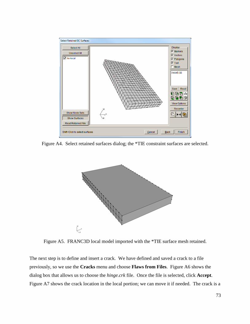
The next dialog, Figure A4, allows one to retain mesh facets. There are no boundary conditions,
but we will retain the *TIE surfaces. Click on the Show Surfaces button and check the tie-local
surface. Note that the tie-local surface was defined in ABAQUS CAE and is part of the local
portion. There is a corresponding tie-global surface for the global portion. Click Finish to
proceed to the FRANC3D main window, Figure A5.
73
Figure A4. Select retained surfaces dialog; the *TIE constraint surfaces are selected.
Figure A5. FRANC3D local model imported with the *TIE surface mesh retained.
The next step is to define and insert a crack. We have defined and saved a crack to a file
previously, so we use the Cracks menu and choose Flaws from Files. Figure A6 shows the
dialog box that allows us to choose the hinge.crk file. Once the file is selected, click Accept.
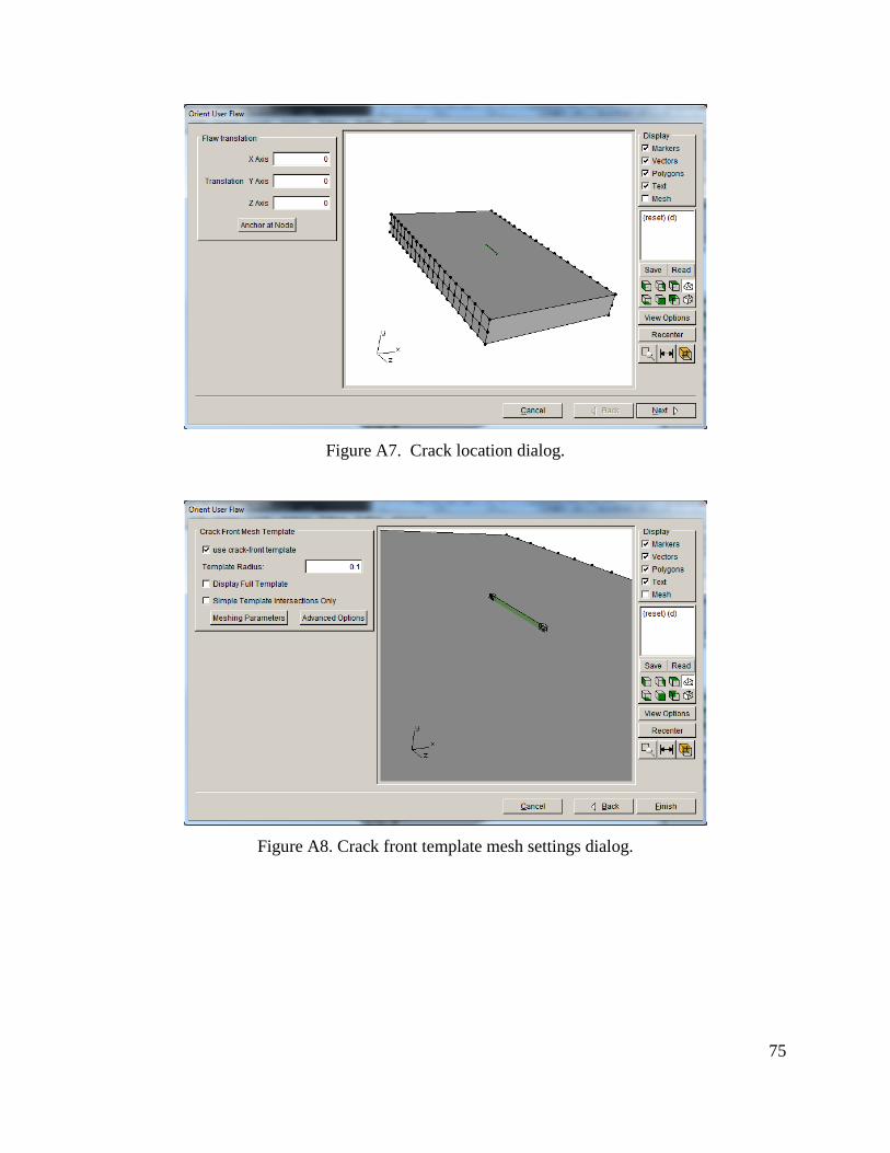
Figure A7 shows the crack location in the local portion; we can move it if needed. The crack is a
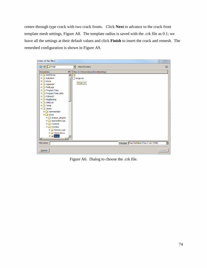
74
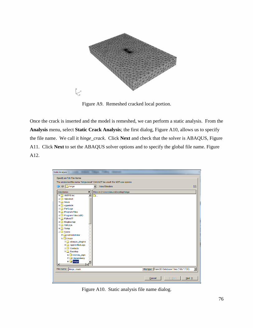
center-through type crack with two crack fronts. Click Next to advance to the crack front
template mesh settings, Figure A8. The template radius is saved with the .crk file as 0.1; we
leave all the settings at their default values and click Finish to insert the crack and remesh. The
remeshed configuration is shown in Figure A9.
Figure A6. Dialog to choose the .crk file.
75
Figure A7. Crack location dialog.
Figure A8. Crack front template mesh settings dialog.
76
Figure A9. Remeshed cracked local portion.
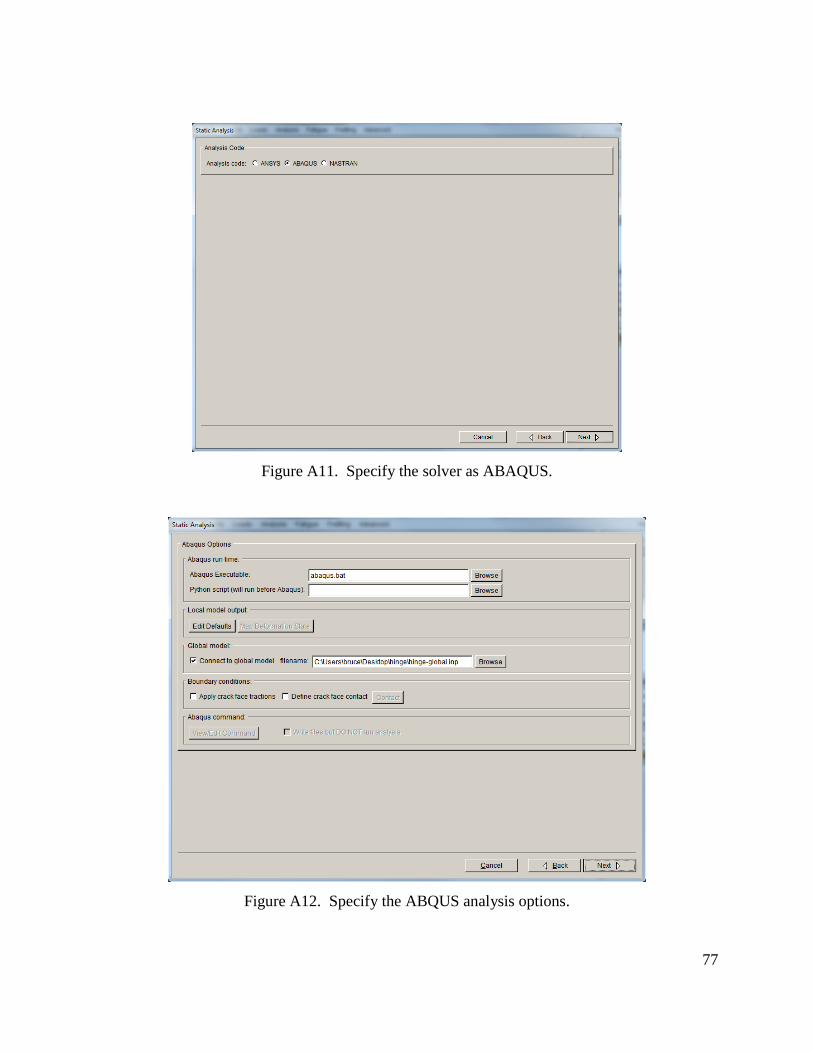
Once the crack is inserted and the model is remeshed, we can perform a static analysis. From the
Analysis menu, select Static Crack Analysis; the first dialog, Figure A10, allows us to specify
the file name. We call it hinge_crack. Click Next and check that the solver is ABAQUS, Figure
A11. Click Next to set the ABAQUS solver options and to specify the global file name. Figure
A12.
Figure A10. Static analysis file name dialog.
77
Figure A11. Specify the solver as ABAQUS.
Figure A12. Specify the ABQUS analysis options.

78
The Global model file name is already filled in by default based on the imported file selection.
Click Next to advance to the next dialog, Figure A13, where we specify how the local and global
model portions will be re-connected. The “tie-local” and “tie-global” surfaces must be selected
along with the Tie constraint option. Click Finish to start the process of saving all of the
analysis files and running ABAQUS in the background. Once ABAQUS finishes running, we
can compute the SIFs and analyze the results to verify that FRANC3D correctly processed all the
ABAQUS information.
Once ABAQUS finishes running, a .dtp file is created, and this file is automatically imported
into FRANC3D. (This assumes that you are running ABAQUS on the same PC as FRANC3D.)
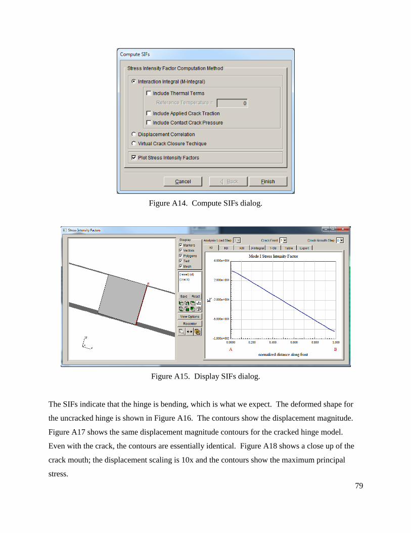
Use the Cracks menu and select Compute SIFs; the dialog shown in Figure A14 is displayed.
Click Finish to display the SIFs for the two crack fronts, Figure A15.
Figure A13. Specify the ABQUS local + global model connection.
79
Figure A14. Compute SIFs dialog.
Figure A15. Display SIFs dialog.
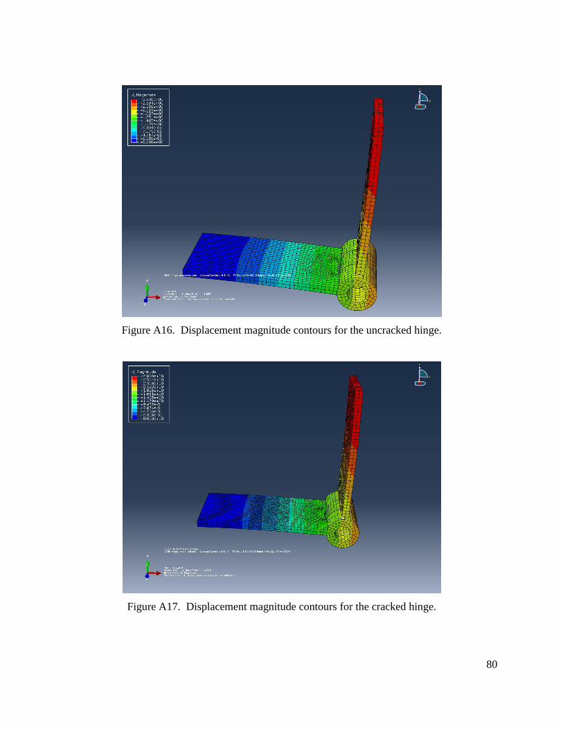
The SIFs indicate that the hinge is bending, which is what we expect. The deformed shape for
the uncracked hinge is shown in Figure A16. The contours show the displacement magnitude.
Figure A17 shows the same displacement magnitude contours for the cracked hinge model.
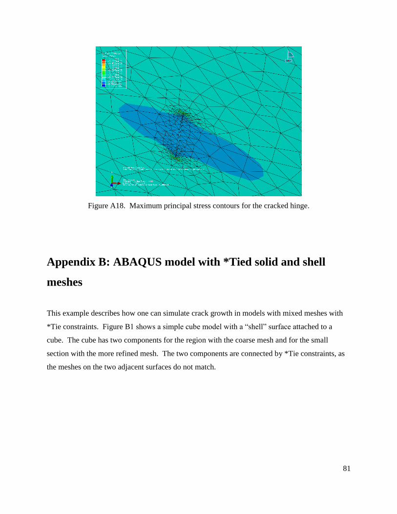
Even with the crack, the contours are essentially identical. Figure A18 shows a close up of the
crack mouth; the displacement scaling is 10x and the contours show the maximum principal
stress.
80
Figure A16. Displacement magnitude contours for the uncracked hinge.
Figure A17. Displacement magnitude contours for the cracked hinge.
81
Figure A18. Maximum principal stress contours for the cracked hinge.
Appendix B: ABAQUS model with *Tied solid and shell
meshes
This example describes how one can simulate crack growth in models with mixed meshes with
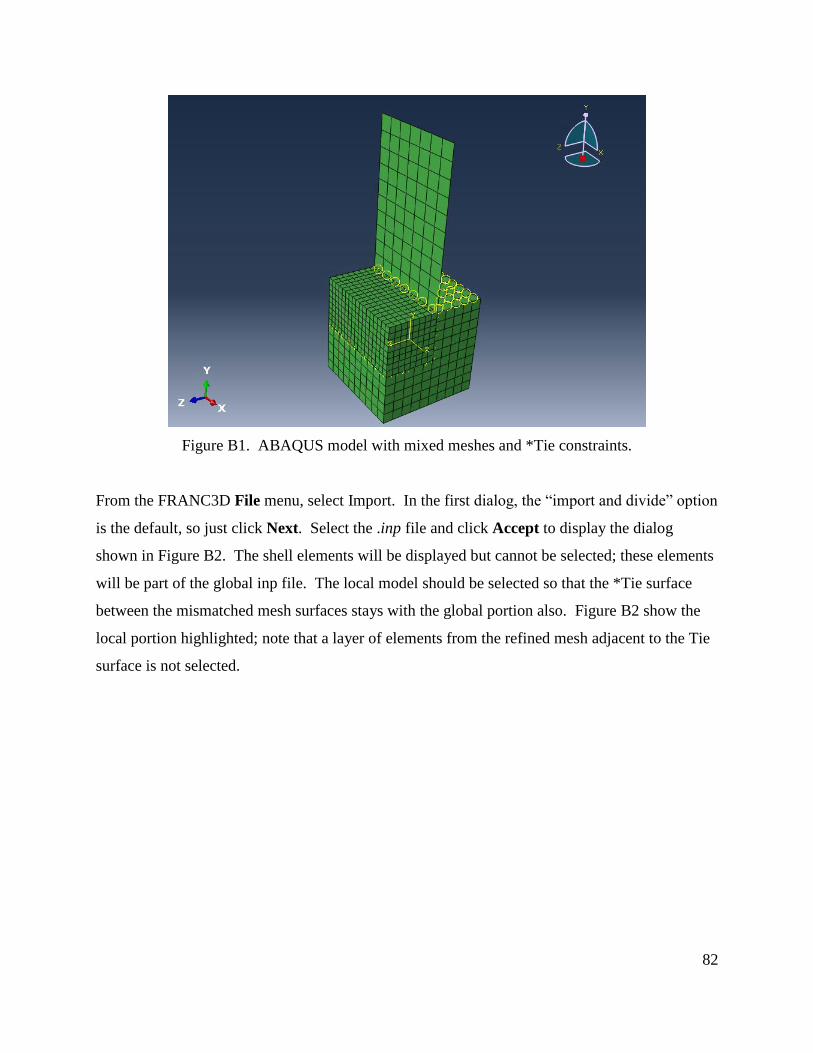
*Tie constraints. Figure B1 shows a simple cube model with a “shell” surface attached to a
cube. The cube has two components for the region with the coarse mesh and for the small
section with the more refined mesh. The two components are connected by *Tie constraints, as
the meshes on the two adjacent surfaces do not match.
82
Figure B1. ABAQUS model with mixed meshes and *Tie constraints.
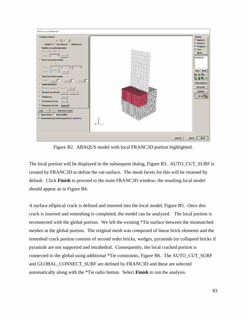
From the FRANC3D File menu, select Import. In the first dialog, the “import and divide” option
is the default, so just click Next. Select the .inp file and click Accept to display the dialog
shown in Figure B2. The shell elements will be displayed but cannot be selected; these elements
will be part of the global inp file. The local model should be selected so that the *Tie surface
between the mismatched mesh surfaces stays with the global portion also. Figure B2 show the
local portion highlighted; note that a layer of elements from the refined mesh adjacent to the Tie
surface is not selected.
83
Figure B2. ABAQUS model with local FRANC3D portion highlighted.
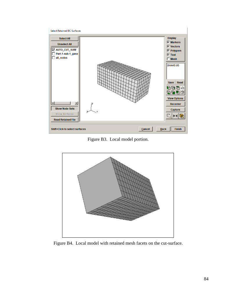
The local portion will be displayed in the subsequent dialog, Figure B3. AUTO_CUT_SURF is
created by FRANC3D to define the cut-surface. The mesh facets for this will be retained by
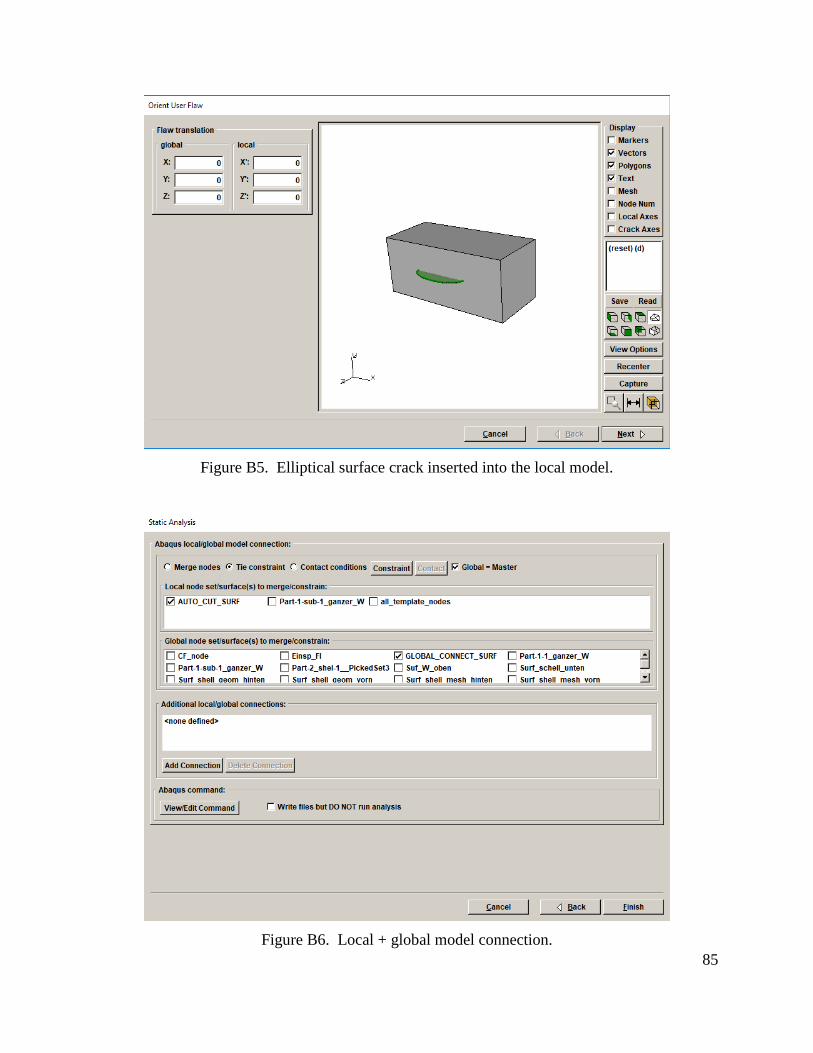
default. Click Finish to proceed to the main FRANC3D window; the resulting local model
should appear as in Figure B4.
A surface elliptical crack is defined and inserted into the local model, Figure B5. Once this
crack is inserted and remeshing is completed, the model can be analyzed. The local portion is
reconnected with the global portion. We left the existing *Tie surface between the mismatched
meshes in the global portion. The original mesh was composed of linear brick elements and the
remeshed crack portion consists of second order bricks, wedges, pyramids (or collapsed bricks if
pyramids are not supported and tetrahedral. Consequently, the local cracked portion is
connected to the global using additional *Tie constraints, Figure B6. The AUTO_CUT_SURF
and GLOBAL_CONNECT_SURF are defined by FRANC3D and these are selected
automatically along with the *Tie radio button. Select Finish to run the analysis.
84
Figure B3. Local model portion.
Figure B4. Local model with retained mesh facets on the cut-surface.
85
Figure B5. Elliptical surface crack inserted into the local model.
Figure B6. Local + global model connection.

86
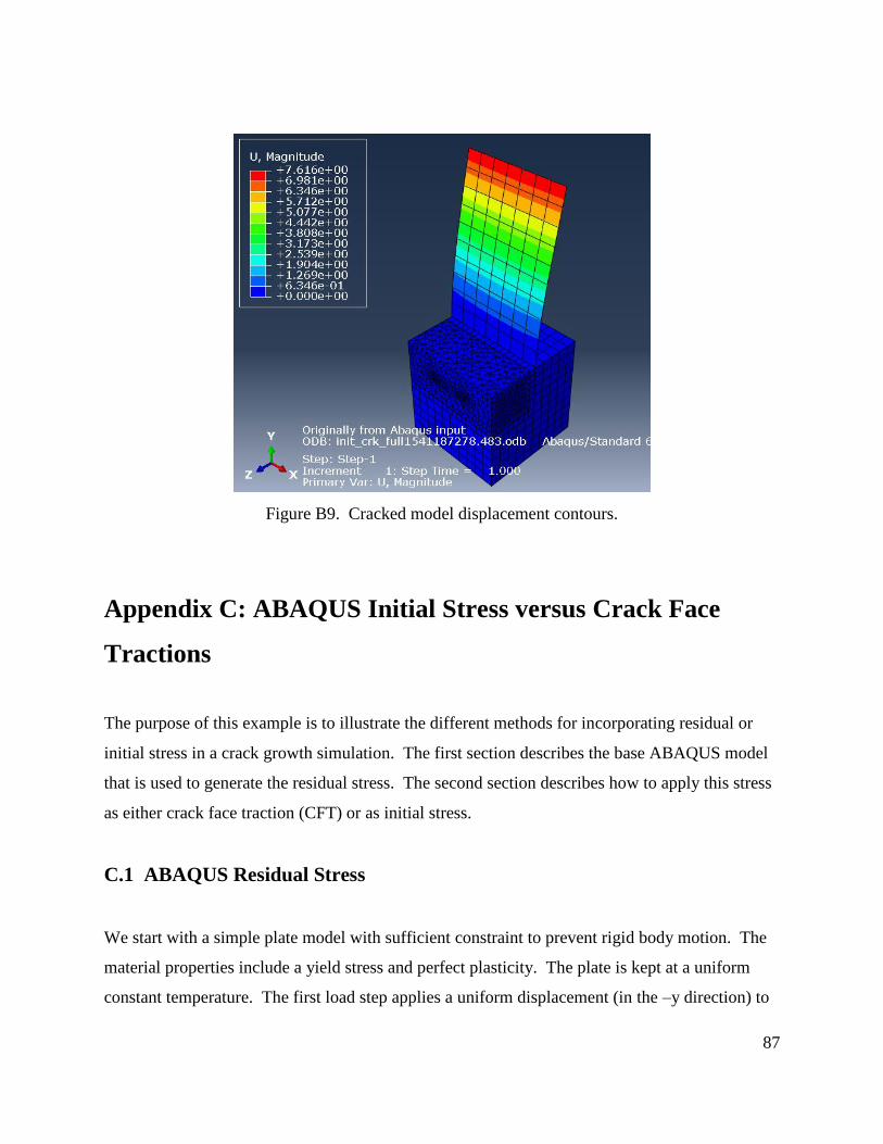
The resulting Mode I SIFs for the crack are shown in Figure B7. The displacement magnitude
contours for the original uncracked and the cracked model are shown in Figures B8 and B9. The
results match reasonably well.
Figure B7. Initial crack Mode I SIFs.
Figure B8. Uncracked model displacement contours.
87
Figure B9. Cracked model displacement contours.
Appendix C: ABAQUS Initial Stress versus Crack Face
Tractions
The purpose of this example is to illustrate the different methods for incorporating residual or
initial stress in a crack growth simulation. The first section describes the base ABAQUS model
that is used to generate the residual stress. The second section describes how to apply this stress
as either crack face traction (CFT) or as initial stress.
C.1 ABAQUS Residual Stress
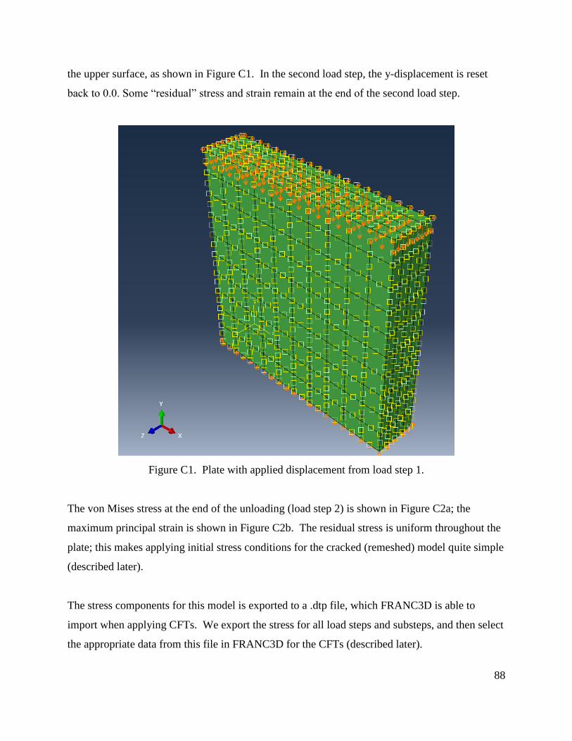
We start with a simple plate model with sufficient constraint to prevent rigid body motion. The
material properties include a yield stress and perfect plasticity. The plate is kept at a uniform
constant temperature. The first load step applies a uniform displacement (in the –y direction) to
88
the upper surface, as shown in Figure C1. In the second load step, the y-displacement is reset
back to 0.0. Some “residual” stress and strain remain at the end of the second load step.
Figure C1. Plate with applied displacement from load step 1.
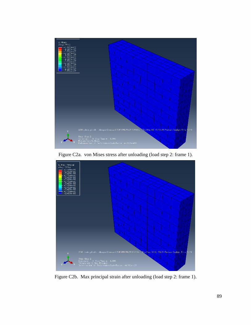
The von Mises stress at the end of the unloading (load step 2) is shown in Figure C2a; the
maximum principal strain is shown in Figure C2b. The residual stress is uniform throughout the
plate; this makes applying initial stress conditions for the cracked (remeshed) model quite simple
(described later).
The stress components for this model is exported to a .dtp file, which FRANC3D is able to
import when applying CFTs. We export the stress for all load steps and substeps, and then select
the appropriate data from this file in FRANC3D for the CFTs (described later).
89
Figure C2a. von Mises stress after unloading (load step 2: frame 1).
Figure C2b. Max principal strain after unloading (load step 2: frame 1).
90
C.2 Residual Stress as Initial Stress
This same plate is used to illustrate how to apply the initial stress conditions in the uncracked
case. This section shows how ABAQUS can apply residual stress as initial conditions using
ABAQUS files – if the mesh is the same.
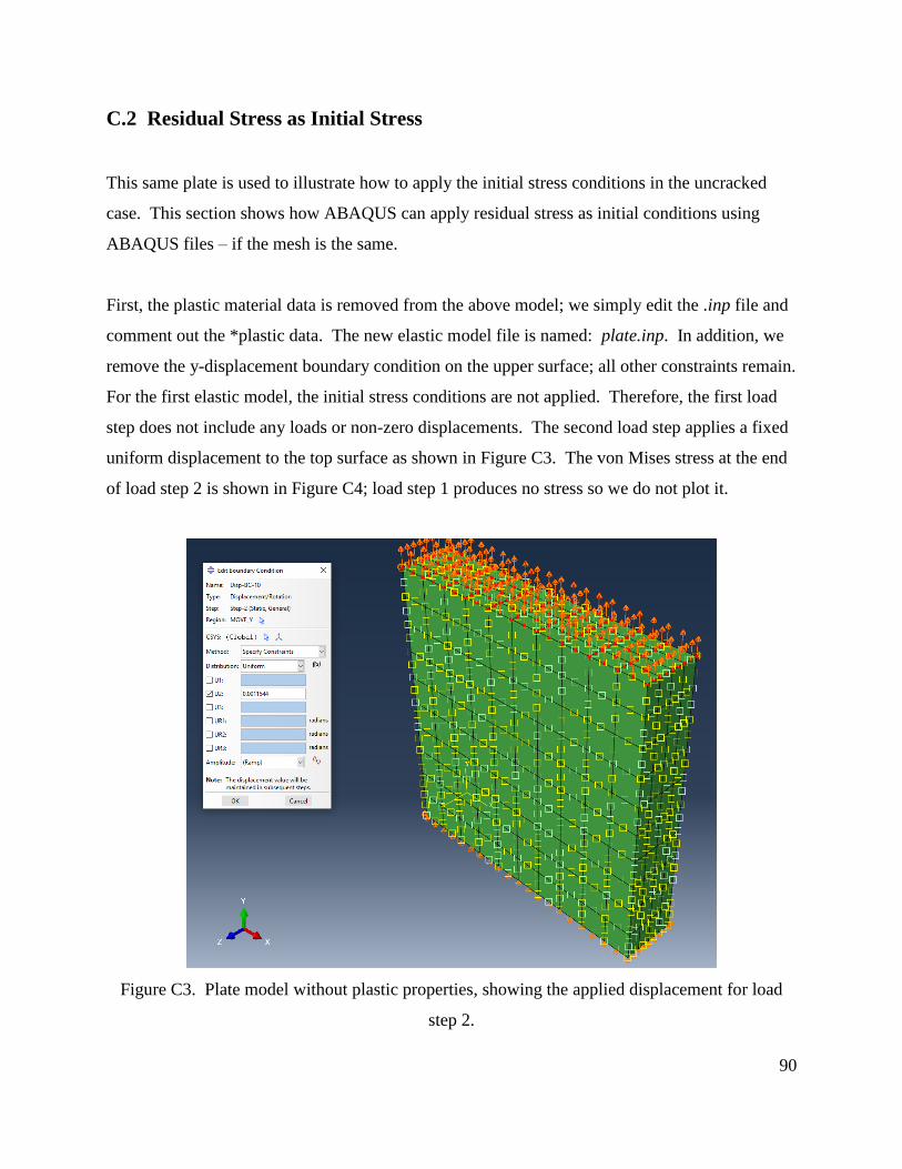
First, the plastic material data is removed from the above model; we simply edit the .inp file and
comment out the *plastic data. The new elastic model file is named: plate.inp. In addition, we
remove the y-displacement boundary condition on the upper surface; all other constraints remain.
For the first elastic model, the initial stress conditions are not applied. Therefore, the first load
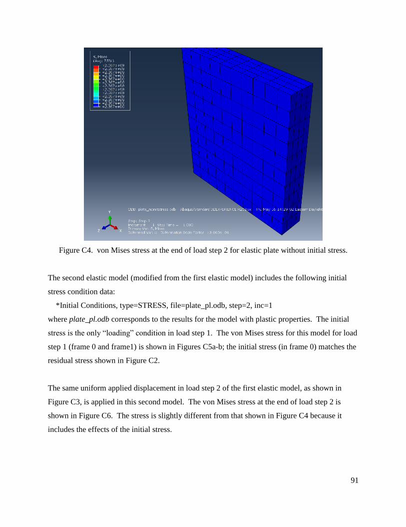
step does not include any loads or non-zero displacements. The second load step applies a fixed
uniform displacement to the top surface as shown in Figure C3. The von Mises stress at the end
of load step 2 is shown in Figure C4; load step 1 produces no stress so we do not plot it.
Figure C3. Plate model without plastic properties, showing the applied displacement for load
step 2.
91
Figure C4. von Mises stress at the end of load step 2 for elastic plate without initial stress.
The second elastic model (modified from the first elastic model) includes the following initial
stress condition data:
*Initial Conditions, type=STRESS, file=plate_pl.odb, step=2, inc=1
where plate_pl.odb corresponds to the results for the model with plastic properties. The initial
stress is the only “loading” condition in load step 1. The von Mises stress for this model for load
step 1 (frame 0 and frame1) is shown in Figures C5a-b; the initial stress (in frame 0) matches the
residual stress shown in Figure C2.
The same uniform applied displacement in load step 2 of the first elastic model, as shown in
Figure C3, is applied in this second model. The von Mises stress at the end of load step 2 is
shown in Figure C6. The stress is slightly different from that shown in Figure C4 because it
includes the effects of the initial stress.

92
Figure C5a. von Mises stress for load step 1 – frame 0 in the elastic plate with initial stress.
Figure C5b. von Mises stress for load step 1 – frame 1 in the elastic plate with initial stress.

93
Figure C6. von Mises stress for load step 2 in the elastic plate with initial stress.
C.3 Residual Stress Included in FRANC3D
This section describes how one can apply a “residual” stress in a FRANC3D simulation.
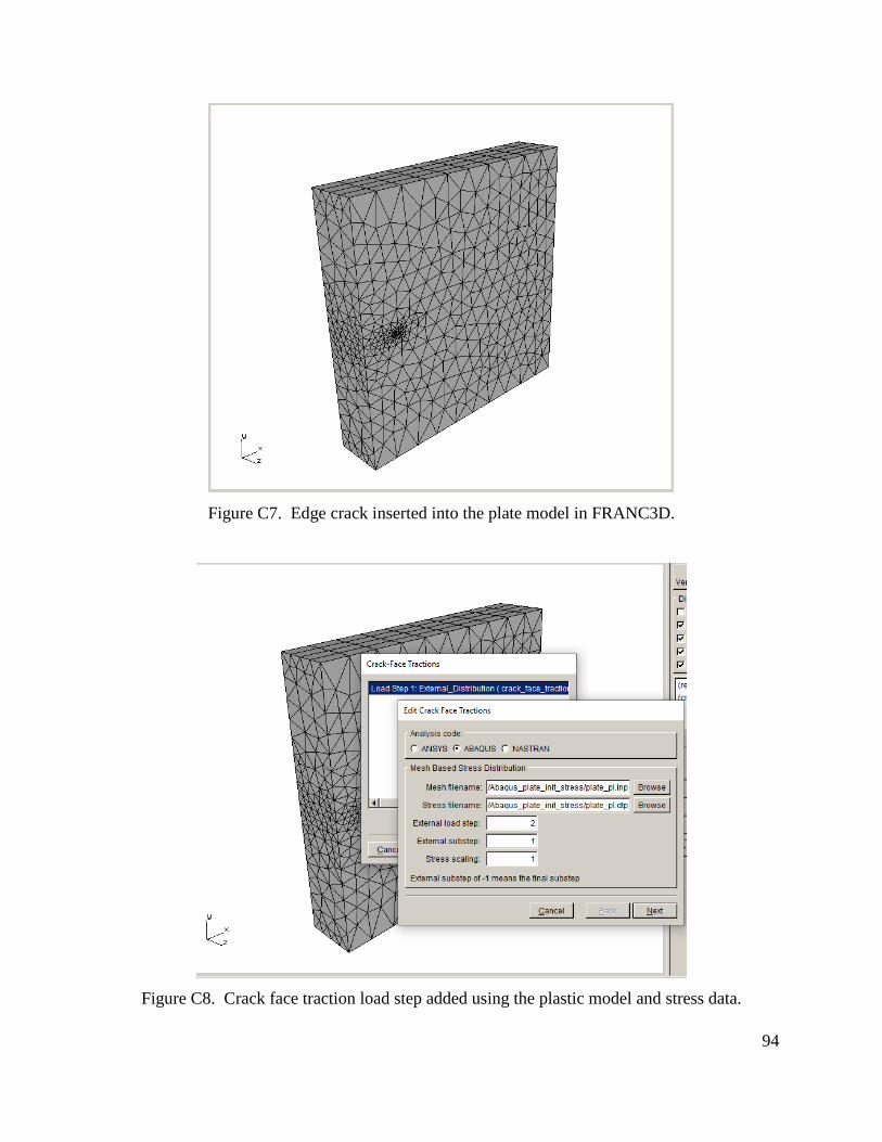
Using the first elastic model (no initial stress), an edge crack is inserted (Figure C7). The
original boundary conditions and load steps are retained. An extra crack face traction (CFT) is
added (Figure C8) using the plastic model mesh file and the “residual” stress from load step 2
(frame 1) of the same plastic model.
94
Figure C7. Edge crack inserted into the plate model in FRANC3D.
Figure C8. Crack face traction load step added using the plastic model and stress data.
95
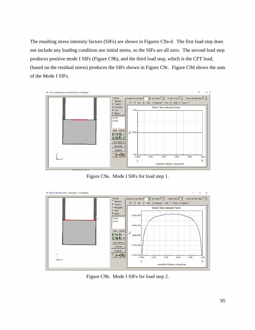
The resulting stress intensity factors (SIFs) are shown in Figures C9a-d. The first load step does
not include any loading condition nor initial stress, so the SIFs are all zero. The second load step
produces positive mode I SIFs (Figure C9b), and the third load step, which is the CFT load,
(based on the residual stress) produces the SIFs shown in Figure C9c. Figure C9d shows the sum
of the Mode I SIFs.
Figure C9a. Mode I SIFs for load step 1.
Figure C9b. Mode I SIFs for load step 2.

96
Figure C9c. Mode I SIFs for load step 3 – the CFT loading.
Figure C9d. Sum of Mode I SIFs.
The same edge crack is inserted into the second elastic model, which includes the initial stress
conditions. The initial stress condition is manually edited in the cracked .inp file to apply a
uniform stress state to all elements:
*Initial Conditions, type=STRESS
all_elements, 0.0, 25000002.0, 0.0, 0.0, 0.0, 0.0
where the stress values are taken from the plastic model “residual” stress state. The resulting
SIFs are shown in Figures C10a-c. Figure C10a shows the SIFs for load step 1 and frame 0,
which are due to the residual stress. Figure C10b shows the SIFs for load step 1 and frame 1,
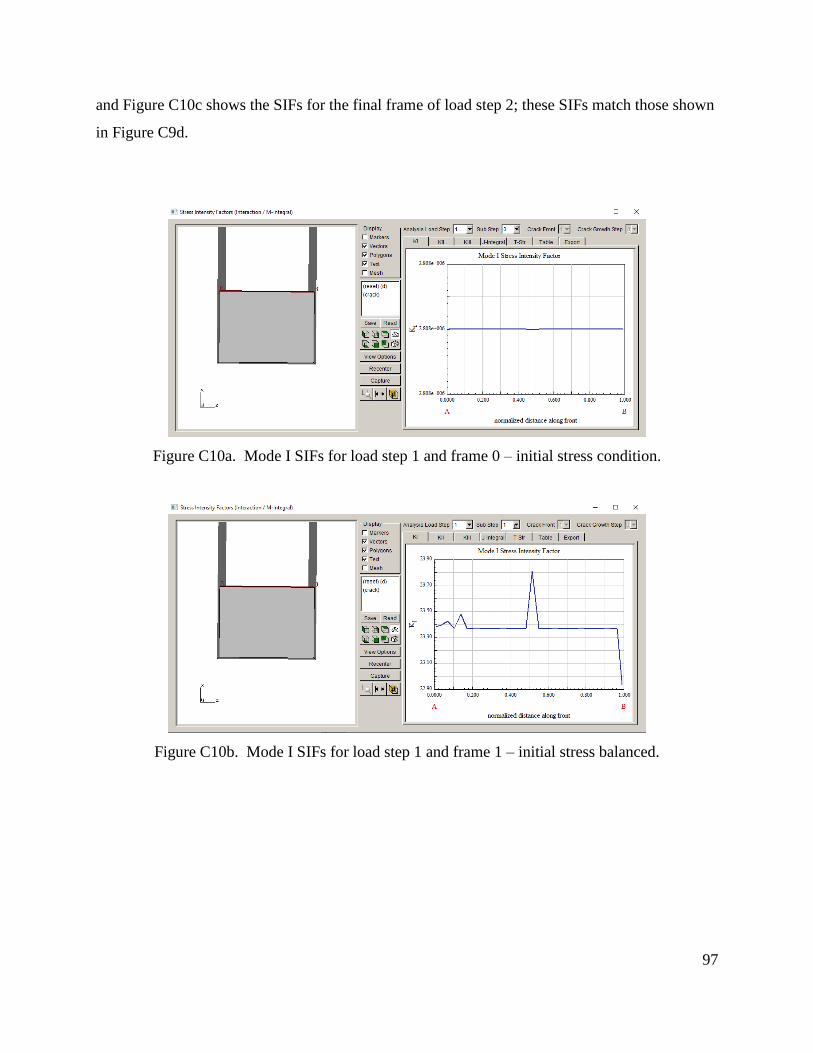
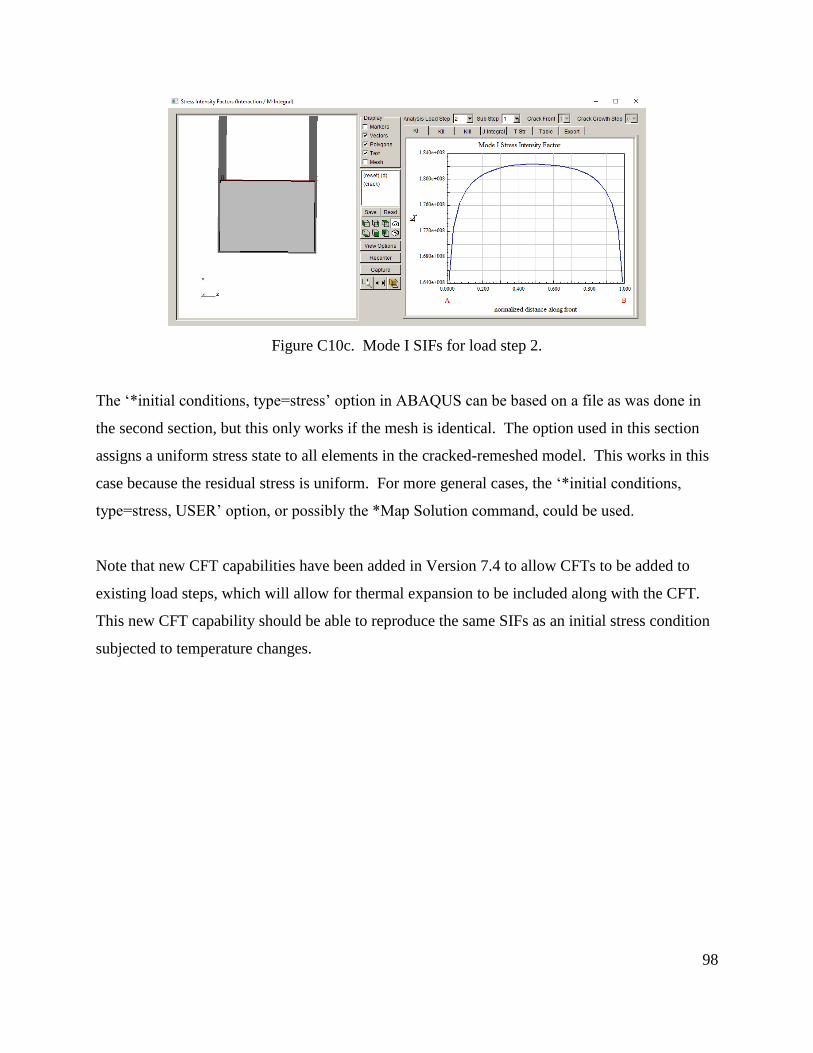
97
and Figure C10c shows the SIFs for the final frame of load step 2; these SIFs match those shown
in Figure C9d.
Figure C10a. Mode I SIFs for load step 1 and frame 0 – initial stress condition.
Figure C10b. Mode I SIFs for load step 1 and frame 1 – initial stress balanced.
98
Figure C10c. Mode I SIFs for load step 2.
The ‘*initial conditions, type=stress’ option in ABAQUS can be based on a file as was done in
the second section, but this only works if the mesh is identical. The option used in this section
assigns a uniform stress state to all elements in the cracked-remeshed model. This works in this
case because the residual stress is uniform. For more general cases, the ‘*initial conditions,
type=stress, USER’ option, or possibly the *Map Solution command, could be used.
Note that new CFT capabilities have been added in Version 7.4 to allow CFTs to be added to
existing load steps, which will allow for thermal expansion to be included along with the CFT.
This new CFT capability should be able to reproduce the same SIFs as an initial stress condition
subjected to temperature changes.