Assessing the performance of global hydrological models

Hydrol. Earth Syst. Sci., 23, 3057–3080, 2019https://doi.org/10.5194/hess-23-3057-2019© Author(s) 2019. This work is distributed underthe Creative Commons Attribution 4.0 License.

Assessing the performance of global hydrological modelsfor capturing peak river flows in the Amazon basinJamie Towner1, Hannah L. Cloke1,2,4,5, Ervin Zsoter3,1, Zachary Flamig6, Jannis M. Hoch7,8, Juan Bazo10,11,Erin Coughlan de Perez9,10, and Elisabeth M. Stephens1

1Department of Geography & Environmental Science, University of Reading, Reading, RG6 6AB, UK2Department of Meteorology, University of Reading, Reading, RG6 6BB, UK3European Centre for Medium-Range Weather Forecasts, Shinfield Park, Reading, RG6 9AX, UK4Department of Earth Sciences, Uppsala University, Uppsala, 752 36, Sweden5Centre of Natural Hazards and Disaster Science, CNDS, Uppsala, 752 36, Sweden6University of Chicago Center for Data Intensive Science, Chicago, USA7Department of Physical Geography, Utrecht University, P.O. Box 80115, 3508 TC Utrecht, the Netherlands8Deltares, P.O. Box 177, 2600 MH Delft, the Netherlands9International Research Institute for Climate and Society, Columbia University, Palisades, NY 10964, USA10Red Cross Red Crescent Climate Centre, 2521 CV The Hague, the Netherlands11Universidad Tecnológica del Perú (UTP), Lima, Peru

Correspondence: Jamie Towner ([email protected])

Received: 29 January 2019 – Discussion started: 27 February 2019Revised: 8 June 2019 – Accepted: 26 June 2019 – Published: 18 July 2019

Abstract. Extreme flooding impacts millions of people thatlive within the Amazon floodplain. Global hydrological mod-els (GHMs) are frequently used to assess and inform themanagement of flood risk, but knowledge on the skill ofavailable models is required to inform their use and develop-ment. This paper presents an intercomparison of eight differ-ent GHMs freely available from collaborators of the GlobalFlood Partnership (GFP) for simulating floods in the Ama-zon basin. To gain insight into the strengths and shortcom-ings of each model, we assess their ability to reproduce dailyand annual peak river flows against gauged observations at75 hydrological stations over a 19-year period (1997–2015).As well as highlighting regional variability in the accuracy ofsimulated streamflow, these results indicate that (a) the me-teorological input is the dominant control on the accuracy ofboth daily and annual maximum river flows, and (b) ground-water and routing calibration of Lisflood based on daily riverflows has no impact on the ability to simulate flood peaksfor the chosen river basin. These findings have important rel-evance for applications of large-scale hydrological models,including analysis of the impact of climate variability, assess-ment of the influence of long-term changes such as land-use

and anthropogenic climate change, the assessment of floodlikelihood, and for flood forecasting systems.

1 Introduction

Flooding is notably the most common and damaging nat-ural hazard affecting millions of people worldwide everyyear, producing economic losses exceeding billions of dol-lars (Hirabayashi et al., 2013). Flood risk associated with aparticular location can be highly variable depending on levelsof exposure, resilience and preparedness (Alfieri et al., 2018),in addition to the increased uncertainty surrounding trendsof hydrological extremes in a warming climate (Arnell andGosling, 2016). For the Amazon basin, flood risk is consid-ered to have increased, with a greater frequency of extremeflood events (e.g. in 2009, 2012, and 2014; Marengo and Es-pinoza, 2016) coinciding with a hypothesized intensificationof the hydrological cycle since the 1980s (Gloor et al., 2013).Floods in Amazonian communities are known to have largesocioeconomic consequences impacting ecosystems, health,and transport links, and are particularly damaging to agri-

Published by Copernicus Publications on behalf of the European Geosciences Union.

3058 J. Towner et al.: Assessing the performance of global hydrological models for capturing peak river flows

cultural and fishery practices (Schöngart and Junk, 2007;Marengo et al., 2012, 2013; Correa et al., 2017). Single floodevents (e.g. 2012 in the Amazonian city of Iquitos, Peru) haveimpacted the lives of over 73 000 people (IFRC, 2013), withaverage annual damages estimated at USD 1.4 billion over a4-year period (2008–2011) in the Brazilian Rio Branco basinalone (Mundial Grupo Banco, 2014).

1.1 Global hydrological models and applications

In its simplest form, a hydrological model can be consid-ered a representation of a real-world hydrological systemused to better understand various water and environmentalprocesses, predict system behaviour, and provide consistentimpact assessment (Devia et al., 2015). They work by simu-lating the hydrological response to meteorological variationsincorporating run-off generation and river routing processes(Sutanudjaja et al., 2018). As such, global hydrological mod-els (GHMs) have been used in a wide range of applications,including short- to extended-range flood forecasting (Alfieriet al., 2013; Emerton et al., 2018), climate assessment (Hat-termann et al., 2017), hazard and risk-mapping (Ward et al.,2015), drought prediction (van Huijevoort et al., 2014), andwater resource assessment (e.g. water availability models;Meigh et al., 1999; Sood and Smakhtin, 2015).

Depending on the application and the needs of decisionmakers, different properties of the hydrograph simulated byhydrological models are important. For example, an accuraterepresentation of peak river flows and their likelihood is keyfor decision-makers who wish to understand the area at riskof flooding. In contrast, estimates of daily streamflow may bemore beneficial for the assessment of water resources such asirrigation requirements.

1.2 GHM development

The availability of GHMs has grown in recent years thanksto increased efforts in addressing water-related issues in de-veloping countries (De Groeve et al., 2015; Ward et al., 2015;Trigg et al., 2016), the development of flood forecasting sys-tems (Aliferi et al., 2013; Werner et al., 2013; Emerton et al.,2018), improvements within precipitation datasets (Mitter-maier et al., 2013; Novak et al., 2014; Forbes et al., 2015),the emergence of new global satellite and remote sensingdatasets, and advancements in numerical modelling tech-niques (Yamazaki et al., 2014a; Sampson et al., 2015; An-dreadis et al., 2017; Balsamo et al., 2018). For an overviewof available GHMs, see Bierkens et al. (2015), who have pro-vided the details of 22 large-scale hydrological models, withthose used for operational flood forecasting being summa-rized in Emerton et al. (2016).

1.3 Land surface models vs. hydrological models

GHMs have differing spatial and temporal resolutions, pa-rameter estimation approaches, number of parameters, cal-ibration methods, input–output variables, and overall struc-tures (Sood and Smakhtin, 2015). Their set-ups can generallybe divided into two categories: land surface models (LSMs)and hydrological models (Gudmundsson et al., 2012). Themajority of LSMs and hydrological models share the sameconceptualization of the water balance (Haddeland et al.,2011) but differ in their objective. LSMs evolve from cou-pled land–atmosphere models with the purpose of solvingthe surface energy balance equations to provide the neces-sary lower boundary conditions to the atmosphere (Wood etal., 2011). In contrast, hydrological models tend to focus lesson the partitioning of radiation and more on hydrological re-sources and understanding the lateral movement and trans-port of water along the land surface.

In terms of differences in model performance, the Gud-mundsson et al. (2012) intercomparison study of six LSMsand five GHMs (i.e. hydrological models) concluded that themain differences were due to the snow scheme implementedwith snow water equivalent values and mean runoff fractionslower in LSMs. No significant differences between LSMsand hydrological models were found for runoff and evap-otranspiration globally, but rather the differences betweenthe models themselves created large sources of uncertainty,highlighting the importance of analysing a range of differ-ent GHMs rather than a group consisting of a specific modeltype. For the purposes of this study, we categorize both LSMand hydrological models as GHMs.

1.4 Motivation

For GHMs to be considered effective, end users need to knowtheir accuracy and reliability (Ward et al., 2015). Thus, theevaluation of these models against observed data is an im-portant procedure in efforts to reduce flood risk. Currently,no intercomparison analysis of GHMs has been conductedspecifically for the Amazon basin, with previous studies fo-cusing solely on the performance of individual models for theAmazon (e.g. Yamazaki et al., 2012; Paiva et al., 2013; Hochet al., 2017a, b) or as part of a global study (e.g. Gudmunds-son et al., 2012; Alfieri et al., 2013; Hirpa et al., 2018), whichlack an in-depth focus on skill within the Amazon basin.

Finally, many of the GHMs (or their components) anal-ysed in this study are used for specific applications, for in-stance, in water resources management (PCRaster GlobalWater Balance; PCR-GLOBWB), flash flood forecasting(Ensemble Framework for Flash Flood Forecasting; EF5),and extended-range flood forecasting (Global Flood Aware-ness System; GloFAS). Investigating the performance of hy-drological simulations therefore can provide valuable in-formation to researchers and model developers with whichto better understand some of the strengths and weaknesses

Hydrol. Earth Syst. Sci., 23, 3057–3080, 2019 www.hydrol-earth-syst-sci.net/23/3057/2019/

J. Towner et al.: Assessing the performance of global hydrological models for capturing peak river flows 3059

which exist within the model set-ups and help to distinguishhow different parts of the hydrological chain can cause par-ticularly “good” or “bad” model performance, thus havingimplications for their different applications.

1.5 Objectives

In this study, the main objective is to assess the ability ofdifferent GHMs freely available from collaborators withinthe Global Flood Partnership (GFP), identifying which ap-proaches are most suitable in different areas of the Amazonbasin for simulating flood peaks. To pursue this objective, theanalysis is designed to answer the following research ques-tions.

1. How well do GHMs represent the annual hydrologicalregime in terms of the Kling–Gupta efficiency (KGE)and its individual components?

2. Which model set-up best represents annual maximumriver flows?

3. Which hydrological routing model allows the best rep-resentation of daily and peak river flows?

4. Which precipitation dataset allows the best representa-tion of daily and peak river flows?

5. How do results differ when using a LSM as opposed toa hydrological model?

6. By how much does calibration of groundwater and rout-ing model parameters improve performance?

2 Data and methodology

The experimental design involves comparing the output ofdaily and annual maximum discharge estimates produced bydifferent GHMs forced using atmospheric reanalysis or satel-lite precipitation datasets against observations of streamflow.The common validation period is 1997–2015, with resultsalso analysed for the shorter period of 2004–2015 to accountfor the shorter record length of one simulation.

2.1 Observations

Observed daily discharge data are used to evaluate each ofthe model runs. The network of hydrometric gauges is con-trolled and maintained by the national institutions responsi-ble for hydrological monitoring in countries situated withinthe Amazon basin. These include the Agência Nacional deÁguas (Water National Office – ANA, Brazil), Servicio Na-cional de Meteorología e Hidrología (National Meteorologyand Hydrology Service – SENAMHI, Peru and Bolivia),Instituto Nacional Meteorologia e Hidrologia (Institute toMeteorology and Hydrology, INAMHI, Ecuador), and the

Instituto de Hidrología, Meteorología y Estudios Ambien-tales (Institute of Hydrology, Meteorology and Environmen-tal Studies – IDEAM, Colombia).

Daily water level values are collected by the respectiveinstitutions and are sourced through the ORE-HYBAM ob-servational service (http://www.ore-hybam.org/, last access:1 December 2018), in collaboration with the Institute of Re-search for Development (IRD) or directly from the nationalservices. A time series of daily river flow for each station isobtained using stage and rating curve measurements whichwere determined using an acoustic Doppler current pro-filer (ADCP) conducted by the ORE-HYBAM observatoryand SENAMHI (Espinoza et al., 2014). In total 75 hydrolog-ical stations throughout the Amazon basin are selected, withan average record length of 17 years within the main valida-tion period (1997–2015). The locations of stations and theircharacteristics are displayed in Fig. 1a and Table S1 in theSupplement respectively. Stations selected have a minimumof 5 consecutive years’ worth of data during the main valida-tion period. The threshold was set to 5 to prevent the elimi-nation of stations in data-scarce areas such as Peru, Bolivia,and Colombia.

2.2 Routing models and meteorological datasets

Eight GHMs composed of different meteorological datasets,hydrological models/LSMs, and river routing models areused to each simulate river discharge across the Amazonbasin. Four meteorological products (ERA-Interim Land re-analysis, ERA-5 re-analysis, European Centre for Medium-range Weather Forecasts (ECMWF) 20-year control refore-casts (hereafter defined as reforecasts), and the real-timeTRMM TMPA 3B42 v.7), three hydrological models/LSMs(PCR-GLOBWB, the Hydrology-Tiled ECMWF Scheme forSurface Exchanges over Land; H-TESSEL, EF5), and threeriver routing models (Catchment-based Macro-scale Flood-plain model, CaMa-Flood; Lisflood; and the Coupled Rout-ing and Excess Storage, CREST) are employed. While thefocus of this study is on GHMs made available by the GFPcommunity, other models are available within the Amazonbasin. Some examples include MGB-IPH (Paiva et al., 2013),LPJmL (Lund–Potsdam–Jena managed Land; Bondeau etal., 2007), WaterGAP (water – global analysis and progno-sis; Döll et al., 2003), and MAC-PDM.09 (the Macro-scale-Probability-Distributed Moisture model.09; Gosling and Ar-nell, 2011).

As a result of using freely available datasets from collab-orators within the GFP, simulations are composed of a com-bination of routing models and meteorological datasets anddo not all use the same precipitation input or hydrologicalset-up. However, the available combinations allow enoughinsight into the model components to draw conclusions forthe objectives stated. For example, to analyse the perfor-mance of precipitation inputs, ERA-Interim Land, ERA-5,and the reforecasts are forced through the calibrated version

www.hydrol-earth-syst-sci.net/23/3057/2019/ Hydrol. Earth Syst. Sci., 23, 3057–3080, 2019

http://www.ore-hybam.org/


Figure 1. (a) Locations of the 75 hydrological gauges and the river network of the Amazon basin. Numbers represent stations which arereferred to throughout the main text in italics. For station information, see Table S1. (b) Locations of existing and under-construction damsas of 2017 (see Latrubesse et al., 2017). (c) Geological map of the Amazon (Schenk et al., 1999). (d) Elevation map of the basin from thedigital elevation model (DEM), GTOPO30, at a horizontal resolution of approximately 1 km (US Geological Survey, 1996).

of Lisflood, whereby the routing and LSM remain consis-tent. To evaluate the differences between using the Lisfloodand CaMa-Flood routing models, two simulations which useERA-Interim Land precipitation and the H-TESSEL LSMare compared. To identify the differences between employ-ing a hydrological model (PCR-GLOBWB) or LSM (H-TESSEL), two set-ups which use the ERA-Interim Landprecipitation reanalysis and the CaMa-Flood river routingmodel are directly compared. Finally, to see how much bene-fit model calibration within Lisflood provides, ERA-InterimLand and ERA-5 are forced through the calibrated and un-calibrated Lisflood model versions. The CREST EF5 run isthe sole simulation to have a unique hydrological model andmeteorological input, and although it is more challenging toanalyse the performance of specific components of the model

set-up against other simulations, it was included in the anal-ysis for completeness.

An alternative approach would be to implement a fullintercomparison experiment and run a new set of simula-tions which included all combinations of precipitation in-put, GHM, and routing scheme. However, this is a verylarge undertaking, and the time and computational expenseto achieve this are prohibitive. Instead, by using freely avail-able datasets with different hydrological set-ups, our methodallows a first analysis providing enough evidence of datasetreliability and accuracy in order to determine the utility ofthe differing approaches for climate studies and to forecastapplications. Moreover, by using iterative runs of similarmodel set-ups (i.e. changing a specific part of the hydrologi-cal model chain), it allows us to make conclusive statements



regarding the differences in skill. Finally, short descriptionsof each model and atmospheric product are outlined below,with a summary of each simulation provided in Table 1.

2.2.1 Precipitation datasets

ERA-Interim Land is a global reanalysis of land surfaceparameters produced by the ECMWF with a T255 spec-tral resolution (∼ 80 km or ∼ 0.75◦; Balsamo et al., 2015).ERA-Interim Land was produced using the latest versionof the land surface H-TESSEL model using atmosphericforcing from ERA-Interim (Dee et al., 2011), with precip-itation adjustments based on the Global Precipitation Cli-mate Project (GPCP) v2.1. Precipitation improvements wereachieved by Balsamo et al. (2010) using a scale-selectiverescaling procedure in which ERA-Interim 3-hourly precipi-tation was corrected to match the monthly accumulation pro-vided by the GPCP at grid point scale (Huffman et al., 2009).All simulations which use ERA-Interim Land are run of-fline to force the associated rainfall–runoff models (see Ta-ble 1). For a detailed description of the ERA-Interim Landand ERA-Interim datasets, see Balsamo et al. (2015) and Deeet al. (2011) respectively. Dataset available at http://apps.ecmwf.int/datasets/data/interim-full-daily/levtype=sfc/ (lastaccess: 1 July 2018).

ERA-5 is the latest reanalysis product of the ECMWFproducing consistent estimates of atmospheric, land, andocean variables at a horizontal resolution of ∼ 31 km, whilethe vertical atmosphere is discretized into 137 levels to0.01 hPa (ECMWF, 2018). ERA-5 is based on the Inte-grated Forecasting System (IFS) Cycle 41r2 which wasused operationally at the ECMWF in 2016. Early analysishas shown that ERA-5 has an improved representation ofprecipitation (particularly over land in the deep tropics),evaporation, and soil moisture compared to its predecessorERA-Interim Land (ECMWF, 2017). ERA-5 is currentlybeing produced in three “streams” and will eventually coverthe period 1950 to near real time (∼ 3 d) with its completiondue in 2019 (Emerton et al., 2018). Dataset available athttps://software.ecmwf.int/wiki/display/CKB/How+to+download+ERA5+data+via+the+ECMWF+Web+API (lastaccess: 1 July 2018).

ECMWF reforecasts are a collection of historical forecastsfrom start dates at the same day of the year going back for aspecific number of years to provide a consistent model clima-tology from which to compare forecasts (ECMWF, 2016).In this study we use the control member of the reforecastswhich are created based on a retrospective run of the mostrecent version of the ECMWF’s IFS to provide surface andsubsurface runoff as input to the Lisflood routing model ata resolution of 0.1◦. The reforecast run is computed usinga lighter configuration (11 ensemble members, run twice aweek on Mondays and Thursdays) to reduce computationaltime. The purpose of running the ECMWF forecasts throughthe Lisflood routing model is to generate a long-term (20-

year) dataset which is consistent with operational GloFASforecasts enabling the suitability of the dataset for use in thecalibration of the Lisflood model parameters (Hirpa et al.,2018). These data cover the period June 1995 to June 2015and due to frequent model updates of the IFS are based onmultiple model cycles: Cycle 41r1 (July through to March)and Cycle 41r2 (March through to June). The control refore-casts from Mondays and Thursdays are used subsequentlyto fill the whole weeks by taking the first 3 and 4 d forecastperiods respectively throughout the 20 years.

TRMM TMPA 3B42 RT v7 is a global merged multi-satellite precipitation product generated at the National Aero-nautics and Space Administration (NASA). TMPA is com-puted for two products: a near-real-time version (TMPA3B42RT v7) and a post-real-time gauged adjusted researchversion (TMPA 3B42 v7), both of which run at resolu-tion of 3-hourly× 0.25◦× 0.25◦ (Huffman et al., 2007). TheTMPA 3B42 RT gridded dataset used in this study coversthe global latitude belt from 60◦ N to 60◦ S. For further in-formation, see Huffman et al. (2007). Dataset available athttps://pmm.nasa.gov/data-access/downloads/trmm (last ac-cess: 4 March 2018).

2.2.2 Hydrological and land surface models

H-TESSEL provides the land surface component of theECMWF IFS (van den Hurk et al., 2000; van den Hurk andViterbo, 2003; Balsamo et al., 2009). H-TESSEL simulatesthe land surface response to atmospheric conditions estimat-ing water and energy fluxes (heat, moisture, and momen-tum) on the land surface (Zsoter et al., 2019). H-TESSELis predominately used within the operational set-up of short-to seasonal-range weather forecasts coupled with the atmo-sphere, but it can also be used in an “offline mode” tocalculate the land surface response to atmospheric forcing,whereby input data (e.g. near-surface meteorological condi-tions) are provided on a 3-hourly time step (Pappenberger etal., 2012). In this study, H-TESSEL receives boundary con-ditions from the atmospheric input provided by either theERA-5 reanalysis, ERA-Interim Land reanalysis, or the re-forecasts providing total runoff for the CaMa-Flood routingmodel, and the surface and sub-surface water fluxes for Lis-flood. Runs forced using the ERA-Interim Land reanalysisare run in the offline mode. For a detailed description of H-TESSEL, see Balsamo et al. (2009).

PCR-GLOBWB is a global hydrological and water re-source model developed at the Department of Physical Ge-ography, Utrecht University, Netherlands (Sutanudjaja et al.,2018). For each grid cell and time step, PCR-GLOBWBsimulates moisture storage in two vertically stacked up-per soil layers, as well as the water exchange among thesoil, the atmosphere, and the underlying groundwater reser-voir. Besides, water demands for irrigation, livestock, in-dustry, and households can be integrated within the model.Run-off is routed along a local drainage direction (LDD)


http://apps.ecmwf.int/datasets/data/interim-full-daily/levtype=sfc/

http://apps.ecmwf.int/datasets/data/interim-full-daily/levtype=sfc/

https://software.ecmwf.int/wiki/display/CKB/How+to+download+ERA5+data+via+the+ECMWF+Web+API

https://software.ecmwf.int/wiki/display/CKB/How+to+download+ERA5+data+via+the+ECMWF+Web+API

https://pmm.nasa.gov/data-access/downloads/trmm


Table1.C

haracteristicsofthe

eightglobalhydrologicalmodels

(GH

Ms)used

toproduce

estimates

ofdailyriverdischarge.

Modelrun

Meteorological

GH

M2

GH

MR

outingR

outingTem

poralStart

End

Calibration

Authors

forcing 1spatial

model 3

spatialresolution

resolutionresolution

ER

A-IL

andE

RA

-ILand

H-T

ESSE

L∼

0.75◦

Lisflood

0.10◦

Daily

1Jan

199731

Dec

2015N

oneB

alsamo

etal.(2015) 1

H-T

ESSE

L(∼

80km

)(∼

10km

)B

alsamo

etal.(2009) 2

Lisflood_uc

vanD

erKnijffetal.(2010) 3

ER

A-IL

andE

RA

-ILand

H-T

ESSE

L∼

0.75◦

Lisflood

0.10◦

Daily

1Jan

199731

Dec

2015See

Hirpa

etB

alsamo

etal.(2015) 1

H-T

ESSE

L(∼

80km

)(∼

10km

)al.(2018)

Balsam

oetal.(2009) 2

Lisflood_c

vanD


ER

A-5

H-T

ESSE

LE

RA

-5H

-TE

SSEL

∼0.28◦

Lisflood

0.10◦

Daily

1Jan

199731

Dec

2015N

oneSee

EC

MW

F(2018) 1

Lisflood_uc

(∼31

km)

(∼10

km)

Balsam

oetal.(2009) 2

vanD


ER

A-5

Lisflood

ER

A-5

H-T

ESSE

L∼

0.28◦

Lisflood

0.10◦

Daily

1Jan

199731

Dec

2015See

Hirpa

etSee

EC

MW

F(2018) 1

H-T

ESSE

L_c

(∼31

km)

(∼10

km)

al.(2018)B

alsamo

etal.(2009) 2

vanD


Reforecasts

EC

MW

F20-year

H-T

ESSE

L∼

0.28◦

Lisflood

0.10◦

Daily

1Jan

199731

Dec

2015See

Hirpa

etSee

EC

MW

F(2017) 1

H-T

ESSE

Lcontrol

(∼31

km)

(∼10

km)

al.(2018)B

alsamo

etal.(2009) 2

Lisflood_c

reforecastsvan

DerK

nijffetal.(2010) 3

ER

A-IL

andE

RA

-ILand

H-T

ESSE

L∼

0.75◦

CaM

a-Flood0.25◦

Daily

1Jan

199731

Dec

2015N

oneB

alsamo

etal.(2015) 1

H-T

ESSE

L(∼

80km

)(∼

25km

)B

alsamo

etal.(2009) 2

CaM

a-FloodY

amazakietal.(2011) 3

ER

A-IL

andE

RA

-ILand

PCR

-∼

0.50◦

CaM

a-Flood0.25◦

Daily

1Jan

199731

Dec

2015N

oneB

alsamo

etal.(2015) 1

PCR

-GL

OB

WB

GL

OB

WB

(∼50

km)

(∼25

km)

Sutanudjajaetal.(2018) 2

CaM

a-FloodY

amazakietal.(2011) 3

TR

MM

TM

PA3B

42v7

EF5/C

RE

ST∼

0.25◦

EF5/C

RE

ST0.05◦

Daily

1Jan

200331

Dec

2015N

oneH

uffman

etal.(2007) 1

CR

EST

EF5

Realtim

e(∼

25km

)(∼

5km

)W

angetal.(2011) 2

Clark

etal.(2016) 3

1M

eteorologicalinputdataset, 2hydrologicalorland

surfacem

odel(LSM

)and3

riverroutingm

odel.The

authorsassociated

with

eachm

odelcomponentare

highlightedby

thesuperscripted

number.



network using the kinematic routing wave equation. PCR-GLOBWB was applied at a resolution of 30 arcmin (∼ 55 km× 55 km at the Equator) with meteorological forcing pro-vided from the ERA-Interim Land reanalysis dataset be-tween 1997 and 2015. For further information on PCR-GLOBWB, see van Beek and Bierkens (2008), van Beek etal. (2011), and Sutanudjaja et al. (2018).

EF5 is an open-source software package developed at theUniversity of Oklahoma (OU) that consists of multiple hy-drological model cores producing outputs of streamflow, wa-ter depth, and soil moisture (Clark et al., 2016). Since 2016,EF5 has been used operationally for local forecasts acrossthe US National Weather Service (NWS) for flash floodingpurposes (Gourely et al., 2017). EF5 incorporates CREST,which is a distributed hydrological model created by OU andNASA (Wang et al., 2011). Within CREST, runoff genera-tion, evapotranspiration, infiltration, and surface and subsur-face routing are computed at each grid cell within the modeldomain, with surface and subsurface water routed using akinematic wave assumption. Four excess storage reservoirscharacterize the vertical profile within a cell representing in-terception by the vegetation canopy and subsurface waterstorage in the three soil layers (Meng et al., 2013). In ad-dition, the representation of sub-grid cell routing and soilmoisture variability is made through the use of two linearreservoirs for overland and subsurface runoff individually(Wang et al., 2011). Locations of major streams, flow direc-tion maps, and flow accumulation are all derived from theHydroSHEDS (Hydrological Data and Maps Based on Shut-tle Elevation Derivatives at Multiple Scales) dataset (Lenhneret al., 2008).

In this study, an un-calibrated version of EF5 was run us-ing CREST version 2.0 (Xue et al., 2013; Zhang et al., 2015)for 13 years (2003–2015), with a 1-year spin-up at a spa-tial resolution of 0.05◦× 0.05◦. Parameters are estimated apriori from soil and geomorphological variables, with me-teorological forcing provided by the TMPA 3B42 RT prod-uct for precipitation and monthly averaged potential evapo-transpiration (PET) from the Food and Agriculture Organi-sation (FAO). For full details on the system set-up, see Clarket al. (2016).

2.2.3 Routing models

Lisflood is a global spatially distributed, grid-based hydro-logical and channel routing model commonly used for thesimulation of large-scale river basins (van Der Knijff et al.,2010). It is currently used as an operational rainfall–runoffmodel within the European Flood Awareness System (EFAS)for streamflow forecasts over Europe (Smith et al., 2016).Unlike EFAS, which uses the full Lisflood set-up, GloFASand the simulations included in this study use only the rout-ing component of the Lisflood set-up, with surface and sub-surface input fluxes (e.g. vertical water, water/snow storage)provided by the H-TESSEL module of the IFS at a resolu-

tion of 0.1◦. Surface runoff is routed through Lisflood usinga four-point implicit finite-difference solution of the kine-matic equations. Sub-surface storage and transport are routedto the nearest downstream channel pixel within one time stepthrough two linear reservoirs (Alfieri et al., 2013). The wa-ter in each channel pixel is finally routed through the rivernetwork taken from the HydroSHEDS project (Lenhner etal., 2008) using the same kinematic wave equations as forthe overland flow. Subsurface flow from the upper and lowergroundwater zones is routed into the nearest downstreamchannel as a scaled sum of the total outflow from both theupper and lower groundwater zones.

Lisflood also represents lakes and reservoirs as simulatedpoints on the river network (Zajac et al., 2017). The outflowsof lakes and reservoirs are based on (a) upstream inflow,(b) precipitation over the lake or reservoir, (c) evaporationfrom the lake or reservoir, (d) the lakes’ initial level, (e) lakeoutlet characteristics, and (f) reservoir-specific characteris-tics. For further details on the parameterization of lakes andreservoirs within Lisflood, see Appendix A within Zajac etal. (2017). In the Amazon, represented lakes are predomi-nately located along the main stem, with very few reservoirsthroughout the basin. For exact lake and reservoir locationswithin the global Lisflood model, see Zajac et al. (2017).

In this study, two set-ups of Lisflood are used (Lisflood_ucand Lisflood_c). Lisflood_c represents the calibrated set-upof the Lisflood routing and groundwater parameters (seeHirpa et al., 2018), while Lisflood_uc represents the uncal-ibrated model run. Parameters were calibrated with the re-forecasts initialized with the ERA-Interim land reanalysisfrom 1995 to 2015 as forcing against observed dischargedata at 1278 gauging stations worldwide. All but one sta-tion (40; see Fig. 1a and Table S1) used in this study wereincluded within the calibration. An evolutionary optimiza-tion algorithm was used to perform the calibration, with theKGE used as the objective function. The calibration was car-ried out for parameters controlling the time constants in theupper and lower zones, percolation rate, groundwater loss,channel Manning’s coefficient, the lake outflow width, thebalance between normal and flood storage of a reservoir, andthe multiplier used to adjust the magnitude of the normal out-flow from a reservoir. The results were validated by Hirpa etal. (2018) using the KGE (Gupta et al., 2009) over the pe-riod 1995–2015. In calibration (validation) KGE skill scoreswere greater than 0.08 compared to the default Lisflood sim-ulation for 67 % (60 %) of stations globally. For a detaileddescription of the calibration of the Lisflood parameters andthe range of values used for each parameter, see Hirpa etal. (2018). Further details of the Lisflood model are describedin van Der Knijff et al. (2010).

CaMa-Flood is a global distributed river routing modelwhich is forced by runoff input from a LSM or hydrolog-ical model to simulate water storage where further hydro-logical variables (i.e. river flow, water level, and inundatedarea) can be derived along a prescribed river network. Hor-



izontal water transport along the river network is calculatedusing the local inertia equations (Yamazaki et al., 2011). Thebackwater effect (i.e. upstream water levels which affect flowvelocity downstream; see Meade et al., 1991) is representedby estimating flow velocity based on water slope (Yamazakiet al., 2011). Moreover, floodplain inundation is representedwithin CaMa-Flood as a subgrid-scale process by discretiz-ing the river basin into unit catchments which consist of sub-grid river and floodplain topography parameters (Yamazakiet al., 2014b). These parameters describe the relationship be-tween the total water storage in each grid point and waterstage and are automatically generated using the Flexible Lo-cation of Waterways (FLOW) method with the generation ofthe river map created by upscaling the HydroSHEDS flowdirection map (Lehner et al., 2008). For further informationabout the CaMa-Flood model, see the aforementioned refer-ences. In this study, daily river discharge was obtained us-ing CaMa-Flood version 3.6.1 at a spatial resolution of 0.25◦

(∼ 25 km grid size) for both runs. Manning’s river and flood-plain roughness coefficients were set at 0.03 and 0.10 s m−1/3

uniformly for both CaMa-Flood simulations.

2.3 Verification metrics

2.3.1 Spearman’s ranked correlation

The non-parametric Spearman ρ is used to measure thestrength and direction of the monotonic relationship betweenthe ranks of the observed and simulated annual maximumvalues. The non-parametric Spearman ρ was preferred toPearson’s statistic as non-parametric measures are less sen-sitive to outliers in the data and are widely considered amore robust measure of the correlation between observed andpredicted values (Legates and McCabe, 1999). Correlationscores for ρ range from − to 1, with 1 being a perfect corre-lation. We consider scores which have a value of 0.6 or moreto be skilful. Similar scores (between 0.5 and 0.7) are consid-ered to represent a good level of agreement between observedand simulated values in similar studies (see Yamazaki et al.,2012; Alfieri et al., 2013).

2.3.2 KGE

The KGE (Gupta et al., 2009) measures the goodness-of-fitbetween estimates of simulated discharge and gauged ob-servations and is a modified version of the dimensionlessNash–Sutcliffe efficiency (NSE; Nash and Sutcliffe, 1970).The metric decomposes the NSE into three independent hy-drograph components – linear correlation (r), bias ratio (β),and relative variability between the observed and simulatedstreamflow (α) – by re-weighting the relative importanceof each (Revilla-Romero et al., 2015). KGE values rangefrom −∞ to 1, with values closer to 1 indicating bettermodel performance. To provide further context to the com-puted KGE scores, we use the breakdown of KGE values

into four benchmark categories as according to (Kling et al.,2012). These are classified as follows:

– “Good” (KGE > 0.75),

– “Intermediate” (0.75>KGE > 0.5),

– “Poor” (0.5>KGE> 0),

– “Very poor” (KGE 6 0).

Although originally for the modified version of the KGE,these categories provide an informative benchmark by whichto evaluate results. A similar study (Thiemig et al., 2013) as-sessing the performance of satellite-based precipitation prod-ucts for hydrological evaluation also adopted the same ap-proach.

When analysing the results, each component of the KGEis also considered independently, enabling model errors tobe directly related to either the variability (KGE_α), biasratio (KGE_β), or correlation (KGE_r; Guse et al., 2017).KGE_α values greater than 1 indicate that variability in thesimulated time series is higher than that observed. Valuesless than 1 show the opposite effect. KGE_β values greaterthan 1 indicate a positive bias whereby predictions overes-timate flows relative to the observed data, while values lessthan 1 represent an underestimation.

To evaluate the relative improvement of using one modelset-up relative to another (e.g. using the calibrated Lisfloodrouting model as opposed to the uncalibrated model version),metrics are calculated as skill scores:

KGESS =KGEa−KGEdef

1−KGEdef, (1)

where KGESS signifies the KGE skill score, KGEa is theKGE score for the improved run or simulation of inter-est (e.g. Lisflood_c), and KGEdef is the KGE score forthe “default” or comparative run (e.g. Lisflood_uc). PositiveKGESS indicates improved skill, whilst a negative score rep-resents a decrease in skill. For each case, KGE scores are cal-culated against observed river flow data. The correlation skillscore is calculated similarly. All metrics are computed in theR environment using the “verification” (Gilleland, 2015) and“hydroGOF” (Zambrano-Bigiarini, 2017) R packages.

3 Results and discussion

To allow for easier interpretation, the results and discus-sion are separated into six sections which match the researchquestions presented in Sect. 1.5, in addition to an outlineof potential future work. Due to similar results between thetwo validation periods (1997–2015 and 2004–2015), only re-sults for 1997–2015 are shown. For 2004–2015 results, seeFigs. S1 and S2 in the Supplement. Results and discussionsfor individual stations are commonly referred to by the sta-tion numbers in italics and are presented in Fig. 1a and Ta-ble S1.



Figure 2. Full Kling–Gupta efficiency (KGE) scores at the 75 hydrological gauging stations for all simulations. For the periods 1997–2015and 2004–2015 for the Coupled Routing and Excess Storage, Ensemble Framework for Flash Flood Forecasting (CREST EF5) run (g).Values greater than 0.75 are considered to indicate good performance (i.e. dark blue circles). To allow for easier model comparisons, plotsare arranged by the different precipitation datasets (rows) and routing models (columns), with the exception of CREST EF5 (g). For example,the final column consists of model runs using the calibrated Lisflood routing model.

3.1 How well is the annual hydrological regimerepresented?

The annual hydrological regime on average is well repre-sented by all models (Fig. 2), with the rationale for poorerperformance at specific gauges dependent on either the tem-poral correlation, bias ratio, or variability ratio componentsof the KGE (Figs. 3–5). An average of 50 % of stations notescores above 0.5 for the KGE metric across all eight simu-lated runs, with a maximum value of 0.92 observed at theSanta Rosa gauging site (48, Fig. 1a) for the ERA-5 Lis-flood_c simulation (Fig. 2f). The two CaMa-Flood set-upsusing the PCR-GLOBWB hydrological model and the H-TESSEL LSM show the lowest skill, with 19 and 18 stationsnoting scores greater than 0.5 respectively. By contrast, thebest performance is from the calibrated Lisflood set-ups, withmedian scores across stations of 0.56, 0.63, and 0.64 for runsforced with ERA-Interim Land, the reforecasts, and ERA-5 respectively. Such results are unsurprising given that theKGE was used as the objective function in the calibrationalgorithm of the Lisflood routing model.

In terms of spatial distribution, the poorest performance isconsistent for the majority of simulations at the Arapari (55),Boca Do Inferno (56), and Base Alalau (61) gauging sta-tions located north of Manaus, at the Fazenda Cajupirangagauge (64) in the northernmost Branco catchment, and atthe Fontanilhas (35) and Indeco (49) stations in the south-eastern Brazilian Amazon (Fig. 2). In the south-eastern Ama-zon, particularly in the Madeira and Tapajos sub-basins, thenumber of existing or under-construction dams is at its high-est (Fig. 1b). Damming of rivers is known to have impactson different aspects of the flow regime, with possible alter-ations in the timing, magnitude, and frequency of low andhigh flows (Magilligan and Nislow, 2005). Indeed, the fre-quency and duration of low- and high-flow pulses at stationsdownstream of dams have been shown to be particularly af-fected by the construction of cumulative dams (Timpe andKaplan, 2017). Thus, discrepancies between observed andmodelled data shown in Fig. 2 could be due to alterationsto key features of the flow regime.

The highest scoring stations (KGE score> 0.75) are pre-dominately found in the south-western Brazilian Amazon



where the network of tributaries remains relatively unaf-fected by damming and where slopes are gentle (Fig. 1band d). However, high skills at stations (32, 33, and 43) alongthe Madeira River for most simulations (Fig. 2) highlightthat the impacts of hydroelectric dams need to be consid-ered on an individual basis, with two of the largest dams(> 3000 MW) situated along the river (see Fig. 1b).

Figures 3–5 show the breakdown of the KGE scores foreach hydrological component to evaluate differences in per-formance with respect to the correlation (i.e. timing), flowvariability (α), and bias ratio (β). An average of 79 % ofstations note correlation coefficients exceeding 0.6 across allruns, with those using the Lisflood routing model performingsimilarly in both spatial distribution and magnitude (Fig. 3).In contrast, 51 % and 47 % of stations achieve values ex-ceeding 0.6 for CaMa-Flood H-TESSEL and CaMa-FloodPCR-GLOBWB respectively, with the hydrological model,PCR-GLOBWB, noting better performance at stations alongthe main stem. The increased performances of Lisflood rela-tive to simulations incorporating CaMa-Flood are likely dueto the increased spatial resolution of the routing component(see Table 1). This is supported by results for CREST EF5,with 76 % of stations noting values above 0.6 and the modeloccupying a finer spatial resolution than that of CaMa-Flood(Fig. 3g).

The variance of modelled river flow is on average higherthan the observed time series in all of the simulations, withthe exception of the ERA-Interim Land PCR-GLOBWBCaMa-Flood simulation. For this run, 85 % of stations ob-serve values of less than one, with stations situated in the Pe-ruvian Amazon (2–5) the notable exception (Fig. 4b). In con-trast, 79 % of stations for the CaMa-Flood set-up using the H-TESSEL LSM note values greater than one (Fig. 4a). All runstend to underestimate river flows relative to the observed timeseries, with the majority of stations observing a beta value ofless than one (Fig. 5). In the calibrated Lisflood simulationforced with the reforecasts, almost half of all the stations ob-serve scores between 0.9 and 1.1 (i.e. grey circles), with amedian of 0.99 (Table 2). These results are not replicated inthe other two calibrated runs when using either ERA-InterimLand or ERA-5 as the precipitation input (Fig. 5d and f). Forboth of these runs a decrease is found in the number of sta-tions achieving scores between 0.9 and 1.1 relative to the as-sociated uncalibrated Lisflood set-ups (Fig. 5c and e). Thisis also highlighted by a decrease in the median scores of thetwo respective runs (Table 2), meaning that a greater waterdeficit exists in the calibrated set-ups.

Stations in the south-eastern Amazon, particularly in theupper reaches of the Teles Pires River (37, 38, and 49), tendto underestimate river flow for most simulations (Fig. 5). Inthis region of the basin precipitation is controlled by frontalsystems in the South Atlantic Convergence Zone (SACZ),which is prevalent during austral summer (Ronchail et al.,2002; Espinoza et al., 2009). In addition, rainfall variabilityin the Amazon is strongest in the south-east, with a distinct

dry season (Paiva et al., 2012; Espinoza et al., 2009). Furtheranalysis could be useful in evaluating seasonal patterns ofmodel performance to establish whether climatological fea-tures such as the SACZ are accurately represented within theprecipitation datasets. Other factors impacting performancein the south-east could be associated with the geology andtopography (Fig. 1c and d). Stations in this area of the basinare located within the Brazilian Shields, composed predom-inately of Precambrian rock, and are characterized by gen-tle slopes and low erosion rates (Filizola and Guyot, 2009).Paiva et al. (2012) demonstrated the importance of accu-rate initial conditions of groundwater state variables in theTapajos and Xingu river basins, particularly for low flows.In comparison, the majority of the central parts of the basinare characterized by tertiary rocks, flat terrain, large flood-plains, and high sediment yields. In these regions (e.g. in thesouth-western Brazilian Amazon), KGE scores are generallyhigher (Fig. 2), with surface water variables (e.g. water lev-els, surface runoff, and floodplain storage) considered moreimportant in hydrological prediction uncertainties (Paiva etal., 2012).

The KGE allows us to make explicit interpretations of thehydrological performance of each model owing to decom-position into correlation, bias, and variability terms (Klinget al., 2012). The results indicate that the required develop-ments to improve the representation of daily river flows arespecific to each individual model and to the area of inter-est. For instance, for the ERA-Interim Land PCR-GLOBWBrun, daily correlation scores (Fig. 3b) showed the model suf-fers in reproducing the temporal dynamics of flow (as mea-sured by r) in northern catchments. Calibration of parame-ters which control the timing of the flood wave (e.g. riverflow velocity) may improve performance, whereas model set-ups incorporating the uncalibrated Lisflood routing modelgenerally had lower KGE values in the east of the basincorresponding to an overestimation of river flow variabil-ity (Fig. 4c and e). For these runs, performance slightly im-proved upon the calibration of the groundwater and routingparameters relating to timing, flow variability, and ground-water loss (Fig. 4d and f).

3.2 Which model set-up best represents annualmaximum river flows?

Both the calibrated and uncalibrated versions of Lisfloodsimulations forced with the ERA-5 reanalysis are the best-performing runs, with median scores of 0.53 and 0.54 for theuncalibrated and calibrated simulations respectively (Fig. 7and Table 2). However, a large deterioration in skill is evi-dent for all simulations for Spearman’s ranked coefficientsbetween observed and predicted annual maximum river flows(Fig. 6), with only 21 % of stations on average observingscores exceeding 0.6 across all simulations. Here, it is im-portant to note that due to the length of some station timeseries the number of overlapping data points can be small,



Figure 3. Correlation component (Pearson’s) of the KGE at the 75 hydrological gauging stations for all simulations. For the periods 1997–2015 and 2004–2015 for the Coupled Routing and Excess Storage, Ensemble Framework for Flash Flood Forecasting (CREST EF5) run (g).Values greater than 0.6 are considered skilful (i.e. blue circles).

Table 2. Median scores for the 75 hydrological gauging stations for all metrics.

Model runs Spearman KGE r Beta Alphaannual max (Pearson’s)correlations

ERA-Interim Land H-TESSEL CaMa-Flood 0.24 0.30 0.61 0.92 1.33ERA-Interim Land PCR-GLOBWB CaMa-Flood 0.23 0.18 0.59 0.98 0.64ERA-Interim Land H-TESSEL Lisflood_uc 0.40 0.51 0.80 0.99 1.25ERA-Interim Land H-TESSEL Lisflood_c 0.42 0.56 0.80 0.86 1.15ERA-5 H-TESSEL Lisflood_uc 0.53 0.63 0.85 0.97 1.26ERA-5 H-TESSEL Lisflood_c 0.54 0.64 0.86 0.87 1.06TRMM CREST EF5 0.24 0.46 0.71 0.80 1.08Reforecasts H-TESSEL Lisflood_c 0.32 0.63 0.83 0.96 1.06Median across models 0.35 0.50 0.78 0.91 1.11

and therefore the spatial distribution of model performanceshould be interpreted with caution. To provide a certainlevel of confidence between results, stations whose time se-ries equals or exceeds 15 years are denoted using a circle,whereas those between 10–14 and 5–9 are represented usinga square and triangle respectively.

The highest scores are generally located towards the east-ern side of the basin and along the main Amazon River where

the terrain is predominately flat, and rivers drain extensivefloodplains. These are constrained to runs using the Lisfloodrouting model with either ERA-Interim Land or ERA-5 asforcing (Fig. 6c–f). Interestingly, the calibrated Lisflood set-up forced using the reforecasts does not replicate good per-formance in these regions (Fig. 6h), indicating that the errorbetween simulated and observed peak river flows could be as-sociated with the precipitation input. When observing daily



Figure 4. Alpha (i.e. variability ratio) component of the KGE at the 75 hydrological gauging stations for all the simulations. For theperiods 1997–2015 and 2004–2015 for the Coupled Routing and Excess Storage, Ensemble Framework for Flash Flood Forecasting(CREST EF5) run (g). Blue circles indicate that the variability in the simulated time series is higher than that of the observed one, while redcircles show the opposite effect. Values closer to one indicate better model performance (i.e. grey circles).

mean precipitation totals over the validation period (1997–2015), the reforecasts observe lower precipitation totals overcentral to northern areas of the basin relative to both of theclimate reanalysis datasets (Fig. 8). However, when compar-ing the results of the ERA-Interim Land H-TESSEL CaMa-Flood and ERA-Interim Land H-TESSEL Lisflood_uc set-ups, correlations are much lower in the CaMa-Flood simula-tion, suggesting that both precipitation and routing processesare equally important (Fig. 6a and c).

Low agreement between peaks is consistent in the south-east and north-west of the basin across all simulations(Fig. 6). In the south-east, a lack of skill could again be asso-ciated with the abundance of hydroelectric dams in the regionor with the poor representation of the SACZ rainfall regime.Evaluating the ability to represent the timing and magnitudeof the annual flood wave has important implications for mod-els predicting flood hazard and for practices providing earlywarning information. These results identify that while therepresentation of daily river flows improves upon model cal-ibration of the Lisflood routing model (Sect. 3.1), the influ-ence of routing calibration for simulating flood peaks has noimpact.

3.3 Which is the best-performing hydrological routingmodel?

We assessed the performance of the CaMa-Flood and Lis-flood_uc routing models by comparing the two runs whichare forced using the ERA-Interim Land reanalysis dataset.On average the uncalibrated Lisflood run outperforms CaMa-Flood for all metrics analysed (Fig. 7 and Table 2). Resultsfrom the CREST EF5 model are also discussed but are notdirectly comparable due to using differing meteorological in-puts.

The median score of the correlation component of theKGE (i.e. Pearson’s correlation coefficient) is found to in-crease by 0.19 when using the un-calibrated Lisflood modelrelative to CaMa-Flood, with 28 more stations achieving acorrelation score of 0.6 or higher (Fig. 3a and c). This num-ber increases when considering correlation scores greaterthan 0.8, with 38 and 7 stations reaching this value for Lis-flood and CaMa-Flood respectively. The most notable in-crease in skill is found in Peru along the Marañón and Naporivers (2 and 5), which note increases of 0.85 and 0.71 re-spectively when using the Lisflood model. In comparison,



Figure 5. Beta (i.e. bias ratio) component of the KGE at the 75 hydrological gauging stations for all the simulations. For the periods 1997–2015 and 2004–2015 for the Coupled Routing and Excess Storage, Ensemble Framework for Flash Flood Forecasting (CREST EF5) run (g).Blue circles indicate that the bias in the simulated time series is higher than that of the observed one, while red circles show the oppositeeffect. Values closer to one indicate better model performance (i.e. grey circles).

the CREST EF5 simulation fits between the CaMa-Flood andLisflood runs with a median daily correlation score of 0.71and notes 12 stations which have scores greater than 0.8(Fig. 3g).

For the overall KGE metric, 24 % and 3 % of stationshave values exceeding 0.5 and 0.75 for CaMa-Flood. Thesefigures rise to 52 % and 11 % respectively in the uncali-brated Lisflood run. Large differences are particularly no-table at stations situated in the upper reaches of the SolimõesRiver (2–6) and within a cluster of stations situated towardsthe Colombian Amazon in the north-west (Fig. 2c). Signifi-cant differences are identified for peak flow correlations, withonly three stations (27, 17, and 22) achieving scores exceed-ing 0.6 for the CaMa-Flood simulation compared to 22 us-ing the uncalibrated Lisflood routing scheme (Fig. 6a and c).In comparison, the CREST EF5 simulation has 11 stationsexceeding this threshold, with no distinguishable spatial pat-tern (Fig. 6g). For this run, the time series of modelled datais shorter (2004–2015), and so peak flow correlations shouldbe interpreted with caution.

Stations located in and around the main Amazon River ob-serve better performance for representing flood peaks in the

Lisflood simulation (Fig. 6c), aligning with the locations oflakes included within the Lisflood set-up (see Zajac et al.,2017). This level of skill was not replicated in the CaMa-Flood simulation, where the representation of lakes is not in-cluded (Fig. 6a), suggesting the potential importance of lakeparameterization for accurate peak flow estimations. How-ever, Zajac et al. (2017) demonstrated that although the in-clusion of lakes in Lisflood was found to generally improvethe representation of extreme discharge for the 5- and 20-year return periods on the global domain, the change in skillupon the inclusion of lakes and reservoirs in the Amazon wasminimal for several metrics. Very few reservoirs are includedwithin Lisflood in the Amazon, and therefore the estimatedeffects on simulated streamflow are restricted.

Zhao et al. (2017) concluded the importance in the choiceof different river routing schemes for simulating peak dis-charge across the globe, while the Hoch et al. (2017b) com-parison of two routing models found results to differ despitehaving identical boundary conditions. It is therefore of in-terest to evaluate not only the entire GHM set-up, but alsoto assess the suitability of each model component of the hy-drological chain in order to determine which routing model



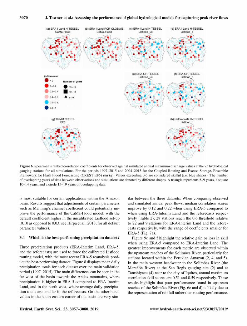
Figure 6. Spearman’s ranked correlation coefficients for observed against simulated annual maximum discharge values at the 75 hydrologicalgauging stations for all simulations. For the periods 1997–2015 and 2004–2015 for the Coupled Routing and Excess Storage, EnsembleFramework for Flash Flood Forecasting (CREST EF5) run (g). Values exceeding 0.6 are considered skilful (i.e. blue shapes). The numberof overlapping years of data between observations and simulations are denoted by different shapes. A triangle represents 5–9 years, a square10–14 years, and a circle 15–19 years of overlapping data.

is most suitable for certain applications within the Amazonbasin. Results suggest that adjustments of certain parameterssuch as Manning’s channel coefficient could potentially im-prove the performance of the CaMa-Flood model, with thedefault coefficient higher in the uncalibrated Lisflood set-up(0.10 as opposed to 0.03; see Hirpa et al., 2018, for all defaultparameter values).

3.4 Which is the best-performing precipitation dataset?

Three precipitation products (ERA-Interim Land, ERA-5,and the reforecasts) are used to force the calibrated Lisfloodrouting model, with the most recent ERA-5 reanalysis prod-uct the best-performing dataset. Figure 8 displays mean dailyprecipitation totals for each dataset over the main validationperiod (1997–2015). The main differences can be seen in thefar west of the basin towards the Andes mountains, whereprecipitation is higher in ERA-5 compared to ERA-InterimLand, and in the north-west, where average daily precipita-tion totals are smaller in the reforecasts. On the other hand,values in the south-eastern corner of the basin are very sim-

ilar between the three datasets. When comparing observedand simulated annual peak flows, median correlation scoresimprove by 0.12 and 0.22 when using ERA-5 compared towhen using ERA-Interim Land and the reforecasts respec-tively (Table 2); 28 stations reach the 0.6 threshold relativeto 22 and 9 stations for ERA-Interim Land and the refore-casts respectively, with the range of coefficients smaller forERA-5 (Fig. 7a).

Figure 9e and f highlight the relative gain or loss in skillwhen using ERA-5 compared to ERA-Interim Land. Thegreatest improvements for each metric are observed withinthe upstream reaches of the Solimões River, particularly forstations located within the Peruvian Amazon (2, 4, and 5).In the main western headwater to the Solimões River (theMarañón River) at the San Regis gauging site (2) and atTamshiyacu (4) near to the city of Iquitos, annual maximumcorrelation skill scores are 0.51 and 0.59 respectively. Theseresults highlight that poor performance found in upstreamreaches of the Solimões River (Fig. 6c and d) is likely due tothe representation of rainfall rather than routing performance.



Figure 7. Boxplots showing the distribution of scores for the (a) Spearman annual maximum correlation, (b) KGE, (c) KGE Pearson’scoefficient, (d) KGE beta, and (e) KGE alpha, for all simulations. For the period 1997–2015.

Figure 8. Mean daily precipitation totals throughout the Amazon basin. For (a) ERA-Interim Land, (b) ERA-5, and (c) the European Centrefor Medium-Range Weather Forecasts (ECMWF) 20-year reforecasts. For the period 1997–2015.

In the other main tributary to the Solimões River, theUcayali River, simulated annual peak flows show little agree-ment with observed data, with a decrease in skill identi-fied when using ERA-5 as opposed to ERA-Interim Land(Fig. 9e). Despite the lack of agreement between observedand modelled data in the Ucayali River, the higher correla-tion scores identified downstream at Tamshiyacu suggest thatbetter representation of high-water periods at the start of theSolimões River is likely modulated by the larger MarañónRiver. Therefore, the ability to represent flood hazard in com-munities near to the city of Iquitos is more dependent on howwell we can predict river flow in the Marañón River.

All three runs perform well for the KGE metric, withlittle difference in results spatially (Fig. 2d, f, h). The re-forecast simulation used within the Lisflood calibration is

found to be superior, with 75 % of stations achieving scoreswhich exceed 0.5 relative to 71 % and 59 % for ERA-5 andERA-Interim Land respectively. Increased skill in the Peru-vian Amazon is again the most noteworthy (Fig. 9f), withKGE skill scores of 0.67 for the Requena (3) (Ucayali River)and San Regis (2) (Marañón River) stations and 0.71 forTamshiyacu (4) (Solimões River) when using ERA-5 rela-tive to ERA-Interim Land. This increase in KGE skill can beattributed to an improvement in the variability and bias ra-tios found between the simulated and observed time series.Daily correlation scores for the three stations (2–4) are nearidentical to the variance and bias ratios underestimated forERA-Interim Land while being much closer to the observeddata for ERA-5 (Figs. 4d, f and 5d, f).



Figure 9. Relative improvement in skill at each gauging station for Spearman annual maximum correlations and KGE values (i.e. skillscores). (a–d) show relative gain or loss in skill when using the calibrated Lisflood run (Lisflood_c) relative to the uncalibrated model run(Lisflood_uc), using precipitation forcing from both ERA-Interim Land and ERA-5. (e) and (f) show the relative gain or loss in skill whenusing ERA-5 as opposed to ERA-Interim Land. (g) and (h) show the relative gain or loss in skill when using the land surface model (LSM),the Hydrology-Tiled ECMWF Scheme for Surface Exchanges over Land (H-TESSEL), compared to the hydrological model, PCRasterGlobal Water Balance (PCR-GLOBWB). All scores are calculated using the skill scores in Eq. (1). Red circles indicate a decrease in skill,whereas blue circles represent an increase.

The Tamshiyacu gauging station (4) is used to measureflood hazard in the city of Iquitos at the start of the SolimõesRiver (Espinoza et al., 2013) and is therefore of particu-lar interest. At this important location, scatterplots of ob-served against simulated river discharge (Fig. 10) show thatthe negative bias observed when using ERA-Interim Landis corrected for when using ERA-5, with the magnitude ofthe 90th percentile of river flows almost identical to that ofthe observed dataset. Improvement is likely associated withthe increased resolution of the ERA-5 reanalysis, which ob-serves higher daily mean precipitation totals in regions to-wards the Andes in the far north-west of the basin (Fig. 8b).Waters found at Tamshiyacu are of Andean origin, meaningthat the representation of rainfall in the Andes Mountainsis fundamental to accurately predicting streamflow. ERA-5runs at a horizontal resolution of ∼ 31 km and includes anadditional 73 vertical levels to 0.01 hPa compared to ERA-

Interim Land, meaning the representation of the troposphereis enhanced (ECMWF, 2017).

The success of GHMs in producing adequate estimates ofriver flow is underpinned by uncertainties within the me-teorological input (Butts et al., 2004; Beven, 2012; Soodand Smakhtin, 2015). These results have particular impor-tance for flood forecasting applications and research con-cerning extreme floods, with the higher-resolution ERA-5dataset providing closer agreement between observed andsimulated annual maximum river flows, particularly for thePeruvian Amazon. With the time series of observed data of-ten beginning in the 1980s in the Amazon, ERA-5 could pro-vide a useful tool for analysing historical flows and estab-lishing links to climate variability. Upon completion, ERA-5will date back to 1950 (Zsoter et al., 2019), meaning loca-tions in which model skill is considered high could benefitfrom up to 30 years’ worth of additional data for use in cli-mate studies, thus allowing for more robust analysis. In fu-



Figure 10. Scatterplots of observed against simulated river flow at the Tamshiyacu gauging site, Peru (4). For (a) ERA-Interim Land,(b) ERA-5, and (c) the European Centre for Medium-Range Weather Forecasts (ECMWF), 20-year reforecasts forced through the calibratedLisflood routing model. Dashed black lines indicate the observed and simulated 90th percentile of river flow. For the period 1997–2015.

ture work, it could be of interest to compare the performanceof ERA-5 against a wider range of precipitation datasets,such as the Multi-Source Weighted-Ensemble Precipitation(MSWEP) product that carefully integrates gauge, satellite,and reanalysis-based estimates. The Beck et al. (2017b) eval-uation of 22 precipitation datasets previously demonstratedthe advantages of using merged products for hydrologicalmodelling purposes.

3.5 How do results differ between using a LSM and ahydrological model?

The H-TESSEL LSM and the PCR-GLOBWB hydrologicalmodel are directly compared whereby the precipitation forc-ing (ERA-Interim Land) and river routing scheme (CaMa-Flood) are consistent. Overall, it appears that the choice be-tween using a LSM or a hydrological model in the Amazonbasin is dependent not only on the specific region of interest,but also on the application and needs of the user. Previousstudies (Zhang et al., 2016; Beck et al., 2017a) have foundthat LSMs, on average, perform better in rainfall-dominantregions, whereas hydrological models tend to achieve bet-ter results in snow-dominated regions owing to the use ofcomplex energy balance equations introducing additional un-certainties. For the Amazon basin, Spearman’s rank correla-tion coefficients between simulated and observed peak riverflow are closely matched, with medians of 0.24 and 0.23for H-TESSEL and PCR-GLOBWB respectively (Table 2).However, the number of stations with Spearman’s maxi-mum correlation scores exceeding 0.6 is slightly higher inPCR-GLOBWB at seven compared to three with H-TESSEL(Fig. 6a and b).

To illustrate the gain or loss in skill when using H-TESSEL relative to PCR-GLOBWB, Spearman’s annualmaximum correlation and KGE skill scores were calculatedfor each station (Fig. 9g and h). Overall, 68 % of the stationsshow improved skill for peak river flow correlations whenusing the LSM, though the gain in skill is minimal (mediancorrelation skill score= 0.06). This percentage drops to 37 %and 22 % for improvements in skill which exceed 0.1 and 0.2respectively (Fig. 9g). By contrast, over half of the stations

see improvements in the KGE skill score for the hydrologi-cal model, PCR-GLOBWB, and 23 % of the stations observeKGE skill score increases which exceed 0.25 (Fig. 9h).

A large loss in performance for the KGE is observed whenusing H-TESSEL for stations in the Peruvian Amazon at theconfluence point to the Solimões River (Fig. 9h). Model per-formance in this region can largely be attributed to the failureof the H-TESSEL CaMa-Flood run to accurately representthe variance of flow and the temporal correlation componentof the KGE, with the variability of modelled flow far higherthan in the observed data (Fig. 4a). Northern regions in theBranco basin and stations situated towards the ColombianAmazon show the opposite effect with higher KGE coeffi-cients found for the H-TESSEL CaMa-Flood run (Fig. 2a),indicating that model suitability is regionally specific.

3.6 By how much does the calibration of groundwaterand routing parameters improve performance?

Calibration of hydrological models is known to be a usefultool in providing more accurate estimates of river flow (Becket al., 2017a). However, due to a lack of data and the compu-tational expense required in the calibration of GHMs, manyremain uncalibrated (Bierkens, 2015; Sood and Smakhtin,2015). Both Gupta et al. (2009) and Mizukami et al. (2019)demonstrate that square error-type metrics are unsuitable formodel calibration when the model in question requires ro-bust performance for high river flows. Improvement of flowvariability estimates was documented in both studies whenswitching the calibration metric from the NSE to the KGEfor both a simple rainfall–runoff model (similar to the HBVmodel; Bergström, 1995) and for two more complex hydro-logical models (Variable Infiltration Capacity and mesoscaleHydrologic Model), suggesting similar results are likely tobe achieved for other hydrological models. To investigate thepotential benefits of routing model calibration, whereby theKGE was used as the objective function, the time series ofriver discharge for the calibrated Lisflood runs forced usingthe ERA-Interim Land and ERA-5 reanalysis datasets werecompared against the associated default set-ups without rout-ing calibration.



Overall, hydrological performance improves upon modelparameter calibration, with positive KGE skill scores (i.e.an increase in skill) at 61 % (59 %) of gauging stations forsimulations forced with ERA-Interim Land (ERA-5) (Fig. 9cand d). The influence of calibration is stronger for the simula-tion forced with ERA-5, with the number of stations achiev-ing “intermediate” KGE scores (i.e. 0.75>KGE > 0.5) to-talling 53 compared to 43 for ERA-Interim Land, an increaseof 9 and 12 stations relative to the associated uncalibratedruns. When observing the spatial distribution of relative im-provements, an east–west divide can be seen (Fig. 9c and d).Generally, decreases in skill are concentrated to stations onthe western side of the basin, whereas stations located to theeast display improved hydrological representation.

Three stations (2–4) in the Peruvian Amazon show in-creased KGE skill scores when using the calibrated ERA-5run relative to the similar uncalibrated set-up (Fig. 9d). Con-versely, a loss in skill is observed at each station for the cal-ibrated run forced using ERA-Interim Land (Fig. 9c). Theseresults are likely associated with a larger negative runoff biaswithin the ERA-Interim Land Lisflood_uc run relative to theERA-5 Lisflood_uc simulation for the three stations (Fig. 5cand e). This is supported by Hirpa et al. (2018), who con-cluded that stations which have a negative streamflow bias inthe default run (i.e. Lisflood_uc) also have a negative KGEskill score in the calibrated simulation owing to the challengeof correcting for a water deficit within the routing compo-nent. Thus, for GHMs which tend to underestimate runoff,adjustments of parameters within the LSM or hydrologicalmodel (e.g. those responsible for the portioning of precipita-tion into runoff) or through bias-correction measures withinthe precipitation dataset may be advantageous in efforts toaccurately represent floods.

No significant differences between calibrated and uncali-brated Lisflood annual maximum correlation scores are iden-tified (Fig. 7a and Table 2). In total, the number of stationsexceeding the 0.6 threshold for peak flow correlations re-mains the same for runs involving ERA-5 and decreases byone for ERA-Interim Land, meaning that the routing modelcalibration has very little impact on the ability to capture an-nual peaks. This suggests that calibrated parameters control-ling flow timing (e.g. Manning’s channel coefficient) are notas important for simulating the magnitude of higher flowsin the Amazon basin and that bias correction of the precip-itation or calibration of parameters associated with runoffand evapotranspiration might be more useful. As previouslyhighlighted by Hirpa et al. (2018), the inclusion of an ob-jective function that is explicitly based on flood peaks couldimprove the ability of Lisflood to simulate floods. This issupported by previous studies (Greuell et al., 2015; Beck etal., 2017a; Mizukami et al., 2019) which have also identi-fied that improved performance in calibrated models is pre-dominately specific to metrics which are incorporated intothe objective function used within the calibration. For in-stance, in Mizukami et al. (2019), they find that when using

an application-specific metric (annual peak flow bias; APFB)for the calibration of two hydrological models, it producedthe best peak flow annual estimates compared to using theNSE, KGE, and its components. However, despite this im-provement, flood magnitudes were still underestimated forall metrics used in calibration, and the use of the APFB asthe calibration metric resulted in poorer performance acrossthe individual KGE components upon evaluation.

3.7 Limitations and future work

While estimating the magnitude of peak river flows is funda-mental, more evaluation is required in assessing the ability torepresent the timing of flood peaks. Modelled flood peakshave been known to occur too early in large Amazonianrivers (Alfieri et al., 2013; Hoch et al., 2017b), with accurateflow timing of significant importance in the Amazon basin.For example, the time displacements between peak flowsin coinciding tributaries are known to play a major role inthe dampening of the Amazon flood wave (Tomasella et al.,2010) and in the synchronization of flood peaks, commonlyassociated with exceptional flood events (e.g. Marengo et al.,2012; Espinoza et al., 2013; Ovando et al., 2016). Additionalevaluation using metrics which focus specifically on the tim-ing aspect, such as the delay index (Paiva et al., 2013), wouldenable a more complete assessment of the hydrological mod-elling regime.

A limitation of this type of study is due to the intercom-parison being restricted to the macroscale (i.e. only a subsetof potential modelling configurations is considered). In fu-ture work it would be useful to increase the granularity of themodelling decision matrix to allow conclusions to be moregeneralized across the modelling community. For instance,when comparing the performance of the Lisflood and CaMa-Flood routing models, the results are specific to the simula-tions forced using the ERA-Interim Land reanalysis dataset.Although useful in providing a general indication of routingperformance for each model when using a climate reanal-ysis dataset, the conclusions are specific to that particularcomparison, with differing results possible when using an-other precipitation input. Future work could investigate oneof the research questions stated in the objectives (Sect. 1.5) ata finer resolution, for example by comparing several differentruns which use the Lisflood and CaMa-Flood routing models,whereby a greater variety of precipitation inputs are consid-ered (e.g. MSWEP, CHIRP V2.0, ERA-5, TRMM v.7). Suchanalysis would allow more general conclusions and recom-mendations to be made to the modelling community, whoare interested in those particular routing schemes. A similarapproach could be adopted for the assessment of other com-ponents of the hydrological modelling chain.



4 Conclusions

In this paper, eight different GHMs were employed in an in-tercomparison analysis using two verification metrics to as-sess model performance against gauged river discharge ob-servations. The motivation for this work stemmed from theneed to evaluate the ability of GHMs to reproduce historicalfloods in the Amazon basin for use in climate analysis and toidentify the strengths and weaknesses which exist along thehydrological modelling chain in order to provide insight tomodel developers. The implications of these results suggestthat the choice of precipitation dataset is the most influen-tial component of the GHM set-up in terms of our ability torecreate annual maximum river flows in the Amazon basin.This is evident with average station correlations between ob-served and simulated annual maximum river flows increas-ing when using the new ERA-5 reanalysis dataset, with sig-nificant improvements in locations of the Peruvian Ama-zon. In this region, waters are sourced from Andean originswhere rainfall can often be poorly represented due to topo-graphically complex terrains (Paiva et al., 2013). Thus, thosewishing to simulate higher flows in the upper reaches of theAmazon may benefit from choosing a precipitation datasetwhich has a high spatial resolution, whereby the upper atmo-sphere is discretized at finer scales. Although an exact recom-mended spatial resolution cannot be provided based on theresults of this study alone, previous works (e.g. Beck et al.,2017b) support the need for a comparatively high-resolutiondataset in addition to other advantageous factors such as along temporal record and the inclusion of daily gauge cor-rections.

Although parameter calibration of the Lisflood routingmodel improved the representation of the whole hydrologi-cal regime across the basin, the agreement between observedand simulated peak discharge values saw no change upon cal-ibration. This indicates that the benefit of calibration is con-fined to the objective function used, in this case the KGE, andhighlights that further model calibration using an objectivefunction that fits the purpose of the application (e.g. RMSEof flood peaks or APFB for flood forecasting systems) couldbe worth considering. It is important to reiterate however thatthoughtful consideration is required if choosing application-specific metrics, with the potential to degrade performance inother aspects of the hydrological regime (e.g. bias and flowvariability ratios) a concern (Mizukami et al., 2019). The rel-ative importance of good performance in the specific targetmetric compared to better performance for a range of metricsshould be assessed on a model-by-model and circumstantialbasis, taking into account the needs of potential users.

Data availability. All of the data and models used in this studywere obtained from collaborators of the Global Flood Partner-ship (GFP) and are freely available. Access to these sources is men-tioned in Sect. 2.

Supplement. The supplement related to this article is availableonline at: https://doi.org/10.5194/hess-23-3057-2019-supplement.

Author contributions. EZ provided data and information for allsimulations incorporating Lisflood and for the ERA-Interim LandH-TESSEL CaMa-Flood set-up. ZF and JM provided data andinformation for the TRMM CREST EF5 and ERA-Interim LandPCR-GLOBWB CaMa-Flood runs respectively. ES, HC, JB, andEC supervised the research and provided important advice. ES,HC, and JT designed the analysis and JT undertook the researchin addition to writing the paper. All the authors were involved indiscussions throughout the development and commented on themanuscript.

Competing interests. The authors declare that they have no conflictof interest.

Acknowledgements. Jamie Towner is grateful for financial sup-port from the Natural Environment Research Council (NERC) aspart of the SCENARIO Doctoral Training Partnership (grant agree-ment NE/L002566/1). The first author is grateful for travel sup-port and funding provided by the Red Cross Red Crescent ClimateCentre, to the research and national services, SO-HYBAM, IRD,SENAMHI, ANA, and INAMHI, for providing observed river dis-charge data, and to the ECMWF for computer access and techni-cal support. Finally, specific thanks go to Christel Prudhomme andthe Environmental Forecasts team in the Evaluation Section at theECMWF for their advice and support throughout the analysis andwriting of the manuscript.

Financial support. This research has been supported by the SCE-NARIO NERC (grant no. NE/L002566/1).

Review statement. This paper was edited by Stacey Archfield andreviewed by Gemma Coxon and Andrew Newman.

References

Alfieri, L., Burek, P., Dutra, E., Krzeminski, B., Muraro, D., Thie-len, J., and Pappenberger, F.: GloFAS – global ensemble stream-flow forecasting and flood early warning, Hydrol. Earth Syst.Sci., 17, 1161–1175, https://doi.org/10.5194/hess-17-1161-2013,2013.

Alfieri, L., Cohen, S., Galantowicz, J., Schumann, G. J., Trigg,M. A., Zsoter, E., Prudhomme, C., Kruczkiewicz, A., Cough-lan de Perez, E., Flamig, Z., Rudari., R., Wu, H., Adler, R. F.,Brakenbridge, R. G., Kettner, A., Weerts, A., Matgen, P., Is-lam, S. A. K. M., and Salamon, P.: A global network for oper-ational flood risk reduction, Environ. Sci. Policy, 84, 149–158,https://doi.org/10.1016/j.envsci.2018.03.014, 2018.

Adreadis, K. M., Schumann, G. J.-P., Stampoulis, D., Bates,P. D., Brakenridge, G. R., and Kettner, A. J.: Can atmo-


https://doi.org/10.5194/hess-23-3057-2019-supplement

https://doi.org/10.5194/hess-17-1161-2013

https://doi.org/10.1016/j.envsci.2018.03.014


spheric reanalysis datasets be used to reproduce floodingover large scales?, Geophys. Res. Lett., 44, 10369–10377,https://doi.org/10.1002/2017GL075502, 2017.

Andreadis, K. M., Schumann, G. J. P., Stampoulis, D., Bates,P. D., Brakenridge, G. R., and Kettner, A. J.: Can Atmo-spheric Reanalysis Data Sets Be Used to Reproduce Flood-ing Over Large Scales?, Geophys. Res. Lett., 44, 10369–10377,https://doi.org/10.1002/2017GL075502, 2017.

Arnell, N. W. and Gosling, S. N.: The impacts of climate change onriver flood risk at the global scale, Climatic Change, 134, 387–401, https://doi.org/10.1007/s10584-014-1084-5, 2016.

Balsamo, G., Beljaars, A., Scipal, K., Viterbo, P., van den Hurk,B., Hirschi, M., and Betts, A. K.: A revised hydrology for theECMWF model: Verification from field site to terrestrial waterstorage and impact in the Integrated Forecast System, J. Hydrom-eteorol., 10, 623–643, https://doi.org/10.1175/2008JHM1068.1,2009.

Balsamo, G., Pappenberger, F., Dutra, E., Viterbo, P., andVan den Hurk, B. J. J. M.: A revised land hydrology in theECMWF model: a step towards daily water flux prediction ina fully-closed water cycle, Hydrol. Process., 25, 1046–1054,https://doi.org/10.1002/hyp.7808, 2010.

Balsamo, G., Albergel, C., Beljaars, A., Boussetta, S., Brun, E.,Cloke, H., Dee, H., Dutra, D., Muñoz-Sabater, J., Pappen-berger, F., de Rosnay, P., Stockdale. T., and Vitart, F.: ERA-Interim/Land: a global land surface reanalysis data set, Hydrol.Earth Syst. Sci., 19, 389–407, https://doi.org/10.5194/hess-19-389-2015, 2015.

Balsamo, G., Agusti-Panareda, A., Albergel, C., Arduini, G., Bel-jaars, A., Bidlot, J., Bousserez, N., Boussetta, S., Brown, A.,Buizza, R., Buontempo, C., Chevallier, F., Choulga, M., Cloke,H., Cronin, M. F., Dahoui, M., De Rosnay, P., Dirmeyer, P.A., Drusch, M., Dutra, E., Ek, M. B., Gentine, P., Hewitt,H., Keeley, S. P. E., Kerr, Y., Kumar, S., Lupu, C., Mahfouf,J. F., McNorton, J., Mecklenburg, S., Mogensen, K., Muñoz-Sabater, J., Orth, R., Rabier, F., Reichle, R., Ruston, B, Pap-penberger, F., Sandu, I., Seneviratne, S. I., Tietsche, S., Trigo,I. F., Uijlenhoet, R., Wedi, N., Woolway, R. L., and Zeng,X.: Satellite and In Situ Observations for Advancing GlobalEarth Surface Modelling: A Review, Remote Sens., 10, 2038,https://doi.org/10.3390/rs10122038, 2018.

Beck, H. E., van Dijk, A. I., de Roo, A., Dutra, E., Fink, G., Orth, R.,and Schellekens, J.: Global evaluation of runoff from ten state-of-the-art hydrological models, Hydrol. Earth Syst. Sci., 21, 2881–2903, https://doi.org/10.5194/hess-21-2881-2017, 2017a.

Beck, H. E., Vergopolan, N., Pan, M., Levizzani, V., van Dijk, A. I.,Weedon, G. P., Brocca, L., Pappenberger, F., Huffman, G. J., andWood, E. F.: Global-scale evaluation of 22 precipitation datasetsusing gauge observations and hydrological modeling, Hydrol.Earth Syst. Sci., 21, 6201–6217, https://doi.org/10.5194/hess-21-6201-2017, 2017b.

Bergström, S.: The HBV model, in: Comput. Model. Watershed Hy-drol., chap. The HBV mo, edited by: Singh, V., Water ResoucesPublications, Highlands Ranch Co., Colorado, USA, 1995.

Beven, K. J.: Rainfall-Runoff Modelling: The Primer, 2nd Edn.,Wiley-Blackwell, Chichester, UK, 2012.

Bierkens, M. F.: Global hydrology 2015: State, trends,and directions, Water Resour. Res., 51, 4923–4947,https://doi.org/10.1002/2015WR017173, 2015.

Bierkens, M. F., Bell, V. A., Burek, P., Chaney, N., Condon, L. E.,David, C. H., de Roo, A., Döll, P., Drost, N., Famigiletti, J. S.,Flörke, M., Gochis, D. J., Houser, P., Hut, R., Keune, J., Kollet,S., Maxwell, R. M., Reager, J. T., Samaniego, L., Sudicky, E.,Sutanudiaia, E. H., van de Giesen, N., Winsemius, H., and Wood,E. F.: Hyper-resolution global hydrological modelling: what isnext? “Everywhere and locally relevant”, Hydrol. Process., 29,310–320, https://doi.org/10.1002/hyp.10391, 2015.

Bondeau, A., Smith, P. C., Zaehle, S., Schaphoff, S., Lucht, W.,Cramer, W., Gerten, D., Lotze-Campen, H., Muller, C., Re-ichstein, M., and Smith, B.: Modelling the role of agriculturefor the 20th century global terrestrial carbon balance, GlobalChange Biol., 13, 679–706, https://doi.org/10.1111/j.1365-2486.2006.01305.x, 2007.

Butts, M. B., Payne, J. T., Kristensen, M., and Madsen, H.: An eval-uation of the impact of model structure on hydrological mod-elling uncertainty for streamflow simulation, J. Hydrol., 298,242–266, https://doi.org/10.1016/j.jhydrol.2004.03.042, 2004.

Clark III, R. A., Flamig, Z. L., Vergara, H., Hong, Y., Gour-ley, J. J., Mandl, D. J., Frye, S., Handy, M., and Patterson,M.: Hydrological modeling and capacity building in the Re-public of Namibia, B. Am. Meteorol. Soc., 98, 1697–1715,https://doi.org/10.1175/BAMS-D-15-00130.1, 2016.

Correa, S. W., de Paiva, R. C. D., Espinoza, J. C., and Col-lischonn, W.: Multi-decadal Hydrological Retrospective: Casestudy of Amazon floods and droughts, J. Hydrol., 549, 667–684,https://doi.org/10.1016/j.jhydrol.2017.04.019, 2017.

Dee, D. P., Uppala, S. M., Simmons, A. J., Berrisford, P., Poli,P., Kobayashi, S., Andrae, U., Balmaseda, M. A., Balsamo, G.,Bauer, P., Bechtold, P., Belijaars, A. C. M., van de Berg, L., Bid-lot, J., Bormann, N., Delsol, C., Dragani, R., Fuentes, M., Geer,A. J., Haimberger, L., Healy, S. B., Hersbach, S., Hólm, E .V.,Isaksen, L., Kallberg, P., Köhler, M., Matricardi, M., McNally,A. P., Mong-Sanz, B. M., Morcrette, J. J., Park, B. K., Peubey,C., de Rosnay, P., Tavolato, C., Thèpaut, J. N., and Vitart, F.: TheERA-Interim reanalysis: Configuration and performance of thedata assimilation system, Q. J. Roy. Meteorol. Soc., 137, 553–597, https://doi.org/10.1002/qj.828, 2011.

De Groeve, T., Thielen-del Pozo, J., Brakenridge, R., Adler, R.,Alfieri, L., Kull, D., Lindsay, F., Imperiali, O., Pappenberger,F., Rudari, R., Salamon, P., Villars, N., and Wyjad, K.: Join-ing forces in a global flood partnership, B. Am. Meteorol. Soc.,96, ES97–ES100, https://doi.org/10.1175/BAMS-D-14-00147.1,2015.

Devia, G. K., Ganasri, B. P., and Dwarakish, G. S.: A re-view on hydrological models, Aquat. Proced., 4, 1001–1007,https://doi.org/10.1016/j.aqpro.2015.02.126, 2015.

Döll, P., Kaspar, F., and Lehner, B.: A global hydrological modelfor deriving water availability indicators: model tuning and vali-dation, J. Hydrol., 270, 105–134, https://doi.org/10.1016/S0022-1694(02)00283-4, 2003.

ECMWF: A brief description of reforecasts, available at:https://confluence.ecmwf.int/display/S2S/A+brief+description+of+reforecasts (last access: 25 September 2018), 2016.

ECMWF: What are the changes from ERA-Interim to ERA5?,available at: https://confluence.ecmwf.int//pages/viewpage.action?pageId=74764925, (last access: 31 August 2018), 2017.

ECMWF: What is ERA-5?, available at: https://confluence.ecmwf.int/display/CKB/What+is+ERA5, last access: 8 October 2018.


https://doi.org/10.1002/2017GL075502

https://doi.org/10.1002/2017GL075502

https://doi.org/10.1007/s10584-014-1084-5

https://doi.org/10.1175/2008JHM1068.1

https://doi.org/10.1002/hyp.7808



https://doi.org/10.3390/rs10122038




https://doi.org/10.1002/2015WR017173


https://doi.org/10.1111/j.1365-2486.2006.01305.x

https://doi.org/10.1111/j.1365-2486.2006.01305.x

https://doi.org/10.1016/j.jhydrol.2004.03.042

https://doi.org/10.1175/BAMS-D-15-00130.1


https://doi.org/10.1002/qj.828


https://doi.org/10.1016/j.aqpro.2015.02.126

https://doi.org/10.1016/S0022-1694(02)00283-4

https://doi.org/10.1016/S0022-1694(02)00283-4

https://confluence.ecmwf.int/display/S2S/A+brief+description+of+reforecasts

https://confluence.ecmwf.int/display/S2S/A+brief+description+of+reforecasts

https://confluence.ecmwf.int//pages/viewpage.action?pageId=74764925

https://confluence.ecmwf.int//pages/viewpage.action?pageId=74764925

https://confluence.ecmwf.int/display/CKB/What+is+ERA5

https://confluence.ecmwf.int/display/CKB/What+is+ERA5


Emerton, R. E., Stephens, E. M., Pappenberger, F., Pagano, T. C.,Weerts, A. H., Wood, A. W., Salamon, P., Brown, J. D., Hierdt,N., Donnelly, C., Baughc, C. A., and Cloke, H. L.: Continen-tal and global scale flood forecasting systems, Wiley Interdis-cip. Rev. Water, 3, 391–418, https://doi.org/10.1002/wat2.1137,2016.

Emerton, R., Zsoter, E., Arnal, L., Cloke, H. L., Muraro, D., Prud-homme, C., Stephens, E. M., Salamon, P., and Pappenberger, F.:Developing a global operational seasonal hydro-meteorologicalforecasting system: GloFAS v2.2 Seasonal v1.0, Geosci.Model Dev., 11, 3327–3346, https://doi.org/10.5194/gmd-11-3327-2018, 2018.

Espinoza, J. C., Ronchail, J., Guyot, J. L., Cochonneau,G., Naziano, F., Lavado, W., De Oliveria, E., Pombosa,R., and Vauchel, P.: Spatio-temporal rainfall variabil-ity in the Amazon basin countries (Brazil, Peru, Bolivia,Colombia, and Ecuador), Int. J. Climatol., 29, 1574–1594,https://doi.org/10.1002/joc.1791, 2009.

Espinoza, J. C., Ronchail, J., Frappart, F., Lavado, W., Santini, W.,and Guyot, J. L.: The major floods in the Amazonas River andtributaries (western Amazon basin) during the 1970–2012 pe-riod: A focus on the 2012 flood, J. Hydrometeorol., 14, 1000–1008, https://doi.org/10.1175/JHM-D-12-0100.1, 2013.

Espinoza, J. C., Marengo, J. A., Ronchail, J., Carpio, J. M.,Flores, L. N., and Guyot, J. L.: The extreme 2014 flood insouth-western Amazon basin: the role of tropical-subtropicalSouth Atlantic SST gradient, Environ. Res. Lett., 9, 124007,https://doi.org/10.1088/1748-9326/9/12/124007, 2014.

Filizola, N. and Guyot, J. L.: Suspended sediment yieldsin the Amazon basin: an assessment using the Brazil-ian national data set, Hydrol. Process., 23, 3207–3215,https://doi.org/10.1002/hyp.7394, 2009.

Forbes, R., Haiden, T., and Magnusson, L.: Improvements inIFS forecasts of heavy precipitation, Meteorology section ofECMWF newsletter No. 144, ECMWF, Reading, UK, 21–26,https://doi.org/10.21957/jxtonky0, 2015.

Gilleland, M. E.: Package ‘verification’, available at: http://cran.utstat.utoronto.ca/web/packages/verification/verification.pdf(last access: 25 September 2018), 2015.

Gloor, M. R. J. W., Brienen, R. J., Galbraith, D., Feldpausch, T.R., Schöngart, J., Guyot, J. L., Espinoza, J. C., Llyod, J., andPhillips, O. L.: Intensification of the Amazon hydrological cycleover the last two decades, Geophys. Res. Lett., 40, 1729–1733,https://doi.org/10.1002/grl.50377, 2013.

Gosling, S. N. and Arnell, N. W.: Simulating current global riverrunoff with a global hydrological model: model revisions, vali-dation, and sensitivity analysis, Hydrol. Process., 25, 1129–1145,https://doi.org/10.1002/hyp.7727, 2011.

Gourley, J. J., Flamig, Z. L., Vergara, H., Kirstetter, P. E., Clark III,R. A., Argyle, E., Arthur, A., Martinaitis, S., Terti, G., Erlingis,J. M., Hong, Y., and Howard, K. W.: The FLASH Project:Improving the tools for flash flood monitoring and predictionacross the United States, B. Am. Meteorol. Soc., 98, 361–372,https://doi.org/10.1175/BAMS-D-15-00247.1, 2017.

Greuell, J. W., Andersson, J., Donnelly, C., Feyen, L., Gerten,D., Ludwig, F., Pisacane, G., Roudier, P., and Schaphoff,S.: Evaluation of five hydrological models across Europeand their suitability for making projections under climate

change Hydrol. Earth Syst. Sci. Discuss., 12, 10289–10330,https://doi.org/10.5194/hessd-12-10289-2015, 2015.

Gudmundsson, L., Wagener, T., Tallaksen, L. M., and Engeland, K.:Evaluation of nine large-scale hydrological models with respectto the seasonal runoff climatology in Europe, Water Resour. Res.,48, W11504, https://doi.org/10.1029/2011WR010911, 2012.

Gupta, H. V., Kling, H., Yilmaz, K. K., and Martinez, G. F.: Decom-position of the mean squared error and NSE performance criteria:Implications for improving hydrological modelling, J. Hydrol.,377, 80–91, https://doi.org/10.1016/j.jhydrol.2009.08.003, 2009.

Guse, B., Pfannerstill, M., Gafurov, A., Kiesel, J., Lehr, C., andFohrer, N.: Identifying the connective strength between modelparameters and performance criteria, Hydrol. Earth Syst. Sci., 21,5663–5679, https://doi.org/10.5194/hess-21-5663-2017, 2017.

Haddeland, I., Clark, D. B., Franssen, W., Ludwig, F., VOß, F.,Arnell, N. W., Bertrand, N., Best, M., Folwell, S., Gerten,D., Gomes, S., Gosling, S. N., Hagemann, S., Hanasaki,N., Harding, R., Heinke, J., Kabat, P., Koirala, S., Oki, T.,Polcher, J., Stacke, T., Viterbo, P., Weedon, G. P., and Yeh,P.: Multimodel estimate of the global terrestrial water bal-ance: Setup and first results, J. Hydrometeorol., 12, 869–884,https://doi.org/10.1175/2011JHM1324.1, 2011.

Hattermann, F. F., Krysanova, V., Gosling, S. N., Dankers, R., Dag-gupati, P., Donnelly, C., Flörke, M., Huang, S., Motovilov, Y.,Buda, S., Yang, T., Müller, C., Leng, G., Tang, Q., Portmann, F.T., Hagemann, S., Gerten, D., Wada, Y., Masaki, Y., Alemayehu,T., Satoh, Y., and Samaniego, L.: Cross-scale intercomparison ofclimate change impacts simulated by regional and global hydro-logical models in eleven large river basins, J. Clim. Change, 141,561–576, https://doi.org/10.1007/s10584-016-1829-4, 2017.

Hirabayashi, Y., Mahendran, R., Koirala, S., Konoshima, L., Ya-mazaki, D., Watanabe, S., Kim, H., and Kanae, S.: Globalflood risk under climate change, Nat. Clim. Change, 3, 816,https://doi.org/10.1038/nclimate1911, 2013.

Hirpa, F. A., Salamon, P., Beck, H. E., Lorini, V., Alfieri, L., Zsoter,E., and Dadson, S. J.: Calibration of the Global Flood AwarenessSystem (GloFAS) using daily streamflow data, J. Hydrol., 566,595–606, https://doi.org/10.1016/j.jhydrol.2018.09.052, 2018.

Hoch, J. M., Haag, A. V., Dam, A. V., Winsemius, H. C., van Beek,L. P., and Bierkens, M. F.: Assessing the impact of hydro-dynamics on large-scale flood wave propagation–a case studyfor the Amazon Basin, Hydrol. Earth Syst. Sci., 21, 117–132,https://doi.org/10.5194/hess-21-117-2017, 2017a.

Hoch, J. M., Neal, J., Baart, F., van Beek, L. P. H., Winsemius, H.,Bates, P., and Bierkens, M. F.: GLOFRIM v1.0 – A globally ap-plicable computational framework for integrated hydrological–hydrodynamic modelling, Geosci. Model Dev., 10, 3913–3929,https://doi.org/10.5194/gmd-10-3913-2017, 2017b.

Huffman, G. J., Bolvin, D. T., Nelkin, E. J., Wolff, D. B.,Adler, R. F., Gu, G., Hong, Y., Bowman, K. P., andStocker, E. F.: The TRMM multisatellite precipitation analy-sis (TMPA): Quasi-global, multiyear, combined-sensor precip-itation estimates at fine scales, J. Hydrometeorol., 8, 38–55,https://doi.org/10.1175/JHM560.1, 2007.

Huffman, G. J., Adler, R. F., Bolvin, D. T., and Gu, G.: Improvingthe global precipitation record: GPCP version 2.1, Geophys. Res.Lett., 36, L17808, https://doi.org/10.1029/2009GL040000, 2009.


https://doi.org/10.1002/wat2.1137

https://doi.org/10.5194/gmd-11-3327-2018

https://doi.org/10.5194/gmd-11-3327-2018

https://doi.org/10.1002/joc.1791

https://doi.org/10.1175/JHM-D-12-0100.1

https://doi.org/10.1088/1748-9326/9/12/124007


https://doi.org/10.21957/jxtonky0

http://cran.utstat.utoronto.ca/web/packages/verification/verification.pdf

http://cran.utstat.utoronto.ca/web/packages/verification/verification.pdf

https://doi.org/10.1002/grl.50377



https://doi.org/10.5194/hessd-12-10289-2015

https://doi.org/10.1029/2011WR010911



https://doi.org/10.1175/2011JHM1324.1

https://doi.org/10.1007/s10584-016-1829-4

https://doi.org/10.1038/nclimate1911



https://doi.org/10.5194/gmd-10-3913-2017

https://doi.org/10.1175/JHM560.1

https://doi.org/10.1029/2009GL040000


IFRC: Disaster Relief Fund (DREF) Peru: Floods, avail-able at: https://reliefweb.int/sites/reliefweb.int/files/resources/MDRPE005du1.pdf (last access: 25 September 2018), 2013.

Kling, H., Fuchs, M., and Paulin, M.: Runoff condi-tions in the upper Danube basin under an ensembleof climate change scenarios, J. Hydrol., 424, 264–277,https://doi.org/10.1016/j.jhydrol.2012.01.011, 2012.

Latrubesse, E. M., Arima, E. Y., Dunne, T., Park, E., Baker,V. R., d’Horta, F. M., Wight, C., Wittmann, F., Zuanon,J., Baker, P. A., Ribas, C. C., Norgaard, R. B., Filizola,N., Ansar, A., Flyvbjerg, B., and Stevaux, J. C.: Dammingthe rivers of the Amazon basin, Nature, 546, 363–369,https://doi.org/10.1038/nature22333, 2017.

Legates, D. R. and McCabe, G. J.: Evaluating the useof “goodness-of-fit” measures in hydrologic and hydrocli-matic model validation, Water Resour. Res., 35, 233–241,https://doi.org/10.1029/1998WR900018, 1999.

Lehner, B., Verdin, K., and Jarvis, A.: New global hydrographyderived from spaceborne elevation data, Eos Trans. Am. Geo-phys. Union, 89, 93–94, https://doi.org/10.1029/2008EO100001,2008.

Magilligan, F. J. and Nislow, K. H.: Changes in hydro-logic regime by dams, Geomorphology, 71, 61–78,https://doi.org/10.1016/j.geomorph.2004.08.017, 2005.

Marengo, J. A. and Espinoza, J. C.: Extreme seasonal droughts andfloods in Amazonia: causes, trends and impacts, Int. J. Climatol.,36, 1033–1050, https://doi.org/10.1002/joc.4420, 2016.

Marengo, J. A., Tomasella, J., Soares, W. R., Alves, L. M., and No-bre, C. A.: Extreme climatic events in the Amazon basin, Theor.Appl. Climatol., 107, 73–85, https://doi.org/10.1007/s00704-011-0465-1, 2012.

Marengo, J. A., Alves, L. M., Soares, W. R., Rodriguez, D. A., Ca-margo, H., Riveros, M. P., and Pabló, A. D.: Two contrasting se-vere seasonal extremes in tropical South America in 2012: floodin Amazonia and drought in northeast Brazil, J. Climate, 26,9137–9154, https://doi.org/10.1175/JCLI-D-12-00642.1, 2013.

Meade, R. H., Rayol, J. M., Da Conceicão, S. C., and Na-tividade, J. R.: Backwater effects in the Amazon Riverbasin of Brazil, Environ. Geol. Water Sci., 18, 105–114,https://doi.org/10.1007/BF01704664, 1991.

Meigh, J. R., McKenzie, A. A., and Sene, K. J.: A grid-based approach to water scarcity estimates for easternand southern Africa, Water Resour. Mange., 13, 85–115,https://doi.org/10.1023/A:1008025703712, 1999.

Meng, J., Li, L., Hao, Z., Wang, J., and Shao, Q.: Suitability ofTRMM satellite rainfall in driving a distributed hydrologicalmodel in the source region of Yellow River, J. Hydrol., 509, 320–332, https://doi.org/10.1016/j.jhydrol.2013.11.049, 2013.

Mittermaier, M., Roberts, N., and Thompson, S. A.: Along-term assessment of precipitation forecast skill usingthe Fractions Skill Score, Meterol. Appl., 20, 176–186,https://doi.org/10.1002/met.296, 2013.

Mizukami, N., Rakovec, O., Newman, A. J., Clark, M. P.,Wood, A. W., Gupta, H. V., and Kumar, R.: On the choiceof calibration metrics for “high-flow” estimation using hy-drologic models, Hydrol. Earth Syst. Sci., 23, 2601–2614,https://doi.org/10.5194/hess-23-2601-2019, 2019.

Mundial Grupo Banco: Lidando com Perdas: opções de ProteçãoFinanceira contra Desastres no Brasil (Dealing with losses:

options of financial protection against disasters in Brazil),available at: http://bibliotecadigital.planejamento.gov.br/xmlui/bitstream/handle/iditem/658/BancoMundial_opcoes_deprote\T1\textbackslash%C3\T1\textbackslash%A7\T1\textbackslash%C3\T1\textbackslash%A3ofinanceiracontradesastresnoBrasil.pdf?sequence=1 (last access: 25 September 2018), 2014.

Nash, J. E. and Sutcliffe, J. V.: River flow forecasting through con-ceptual models part I – A discussion of principles, J. Hydrol., 10,282–290, https://doi.org/10.1016/0022-1694(70)90255-6, 1970.

Novak, D. R., Bailey, C., Brill, K. F., Burke, P., Hogsett, W.A., Rausch, R., and Schichtel, M.: Precipitation and temper-ature forecast performance at the Weather Prediction Center,Weather Forecast., 29, 489–504, https://doi.org/10.1175/WAF-D-13-00066.1, 2014.

Ovando, A., Tomasella, J., Rodriguez, D. A., Martinez, J. M.,Siqueira-Junior, J. L., Pinto, G. L. N., Passy, P., Vauchel, P.,Noriega, L., and von Randow, C.: Extreme flood events in theBolivian Amazon wetlands, J. Hydrol.: Reg. Stud., 5, 293–308,https://doi.org/10.1016/j.ejrh.2015.11.004, 2016.

Paiva, R. C. D., Collischonn, W., Bonnet, M. P., and De Gonçalves,L. G. G.: On the sources of hydrological prediction uncer-tainty in the Amazon, Hydrol. Earth Syst. Sci., 16, 3127–3137,https://doi.org/10.5194/hess-16-3127-2012, 2012.

Paiva, R. C. D., Buarque, D. C., Collischonn, W., Bonnet,M. P., Frappart, F., Calmant, S., and Mendes, C. A. B.:Large-scale hydrologic and hydrodynamic modeling of theAmazon River basin, Water Resour. Res., 49, 1226–1243,https://doi.org/10.1002/wrcr.20067, 2013.

Pappenberger, F., Dutra, E., Wetterhall, F., and Cloke, H. L.: Deriv-ing global flood hazard maps of fluvial floods through a phys-ical model cascade, Hydrol. Earth Syst. Sci., 16, 4143–4156,https://doi.org/10.5194/hess-16-4143-2012, 2012.

Revilla-Romero, B., Beck, H. E., Burek, P., Salamon, P.,de Roo, A., and Thielen, J.: Filling the gaps: Cali-brating a rainfall-runoff model using satellite-derived sur-face water extent, Remote Sens. Environ., 171, 118–131,https://doi.org/10.1016/j.rse.2015.10.022, 2015.

Ronchail, J., Cochonneau, G., Molinier, M., Guyot, J. L., Chaves, A.G. D. M., Guimarães, V., and De Oliveira, E.: Interannual rain-fall variability in the Amazon basin and sea-surface temperaturesin the equatorial Pacific and the tropical Atlantic Oceans, Int. J.Climatol., 22, 1663–1686, https://doi.org/10.1002/joc.815, 2002.

Sampson, C. C., Smith, A. M., Bates, P. D., Neal, J.C., Alfieri, L., and Freer, J. E.: A high-resolution globalflood hazard model, Water Resour. Res., 51, 7358–7381,https://doi.org/10.1002/2015WR016954, 2015.

Schenk, C. J., Roland, J., Viger, R. J., and Anderson, C. P.:Maps showing geology, oil and gas fields, and geologicprovinces of the South America Region, USGS open-file re-port 97-470D, US Department of the Interior, Denver, USA,https://doi.org/10.3133/ofr97470D, 1999.

Schöngart, J. and Junk, W. J.: Forecasting the flood-pulse in Cen-tral Amazonia by ENSO-indices, J. Hydrol., 335, 124–132,https://doi.org/10.1016/j.jhydrol.2006.11.005, 2007.

Smith, P., Pappenberger, F., Wetterhall, F., Thielen, J., Krzeminski,B., Salamon, P., Muraro, D., Kalas, M., and Baugh, C.: On theoperational implementation of the European Flood AwarenessSystem (EFAS), ECMWF Tech. Memorandum 778, ECMWF,Reading, UK., 1–34, 2016.


https://reliefweb.int/sites/reliefweb.int/files/resources/MDRPE005du1.pdf

https://reliefweb.int/sites/reliefweb.int/files/resources/MDRPE005du1.pdf


https://doi.org/10.1038/nature22333

https://doi.org/10.1029/1998WR900018

https://doi.org/10.1029/2008EO100001

https://doi.org/10.1016/j.geomorph.2004.08.017


https://doi.org/10.1007/s00704-011-0465-1

https://doi.org/10.1007/s00704-011-0465-1

https://doi.org/10.1175/JCLI-D-12-00642.1

https://doi.org/10.1007/BF01704664

https://doi.org/10.1023/A:1008025703712


https://doi.org/10.1002/met.296


http://bibliotecadigital.planejamento.gov.br/xmlui/bitstream/handle/iditem/658/Banco Mundial_opcoes_de prote%C3%A7%C3%A3o financeira contra desastres no Brasil.pdf?sequence=1





https://doi.org/10.1016/0022-1694(70)90255-6

https://doi.org/10.1175/WAF-D-13-00066.1

https://doi.org/10.1175/WAF-D-13-00066.1

https://doi.org/10.1016/j.ejrh.2015.11.004


https://doi.org/10.1002/wrcr.20067


https://doi.org/10.1016/j.rse.2015.10.022


https://doi.org/10.1002/2015WR016954

https://doi.org/10.3133/ofr97470D



Sood, A. and Smakhtin, V.: Global hydrological mod-els: a review, Hydrolog. Sci. J., 60, 549–565,https://doi.org/10.1080/02626667.2014.950580, 2015.

Sutanudjaja, E. H., Beek, R. V., Wanders, N., Wada, Y., Bosmans,J. H., Drost, N., van der Ent, R. J., de Graaf, I. E. M., Hoch, J.M., de Jong, K., Karssenberg, D., López López, P., Peßenteiner,S., Schmitz, O., Straatsma, M. W., Vannametee, E., Wisser, D.,and Bierkens, M. F. P. N.: PCR-GLOBWB 2: a 5 arcmin globalhydrological and water resources model, Geosci. Model Dev., 11,2429–2453, https://doi.org/10.5194/gmd-11-2429-2018, 2018.

Thiemig, V., Rojas, R., Zambrano-Bigiarini, M., and De Roo, A.:Hydrological evaluation of satellite-based rainfall estimates overthe Volta and Baro-Akobo Basin, J. Hydrol., 499, 324–338,https://doi.org/10.1016/j.jhydrol.2013.07.012, 2013.

Timpe, K. and Kaplan, D.: The changing hydrol-ogy of a dammed Amazon, Sci. Adv., 3, e1700611,https://doi.org/10.1126/sciadv.1700611, 2017.

Tomasella, J., Borma, L. S., Marengo, J. A., Rodriguez, D. A.,Cuartas, L. A., Nobre, C., and Prado, M. C.: The droughtsof 1996–1997 and 2004–2005 in Amazonia: hydrological re-sponse in the river main-stem, Hydrol. Process., 25, 1228–1242,https://doi.org/10.1002/hyp.7889, 2010.

Trigg, M. A., Birch, C. E., Neal, J. C., Bates, P. D., Smith, A.,Sampson, C. C., Yamazaki, D., Hirabayashi, Y., Pappenberger,F., Dutra, E., Ward, P. J., Winsemius, H. C., Salamon, P., Dot-torri, F., Rudari, R., Kappes, M. S., Simpson, A. L., Hadzi-lacos, G., and Fewtrell, T. J.: The credibility challenge forglobal fluvial flood risk analysis, Environ. Res. Lett., 11, 094014,https://doi.org/10.1088/1748-9326/11/9/094014, 2016.

US Geological Survey.: Global 30 Arc-Second Eleva-tion (GTOPO30), US Geological Survey, Center for EarthResources Observation and Science (EROS), available at:https://www.usgs.gov/centers/eros/science/usgs-eros-archive-digital-elevation-global-30-arc-second (last access: 6 June 2019),1996.

van Beek, L. P. H. and Bierkens, M. F. P.: The Global Hydrologi-cal Model PCR-GLOBWB: Conceptualization, Parameterizationand Verification, available at: http://vanbeek.geo.uu.nl/suppinfo/vanbeekbierkens2009.pdf (last access: 3 September 2018), 2008.

van Beek, L. P. H., Wada, Y., and Bierkens, M. F. P.:Global monthly water stress: 1. Water balance andwater availability, Water Resour. Res., 47, W07517,https://doi.org/10.1029/2010WR009791, 2011.

van den Hurk, B. J. and Viterbo, P.: The Torne-Kalix PILPS 2 (e)experiment as a test bed for modifications to the ECMWFland surface scheme, Global Planet. Change, 38, 165–173,https://doi.org/10.1016/S0921-8181(03)00027-4, 2003.

van den Hurk, B. J. J. M., Viterbo, P., Beljaars, A. C. M., and Betts,A. K.: Offline validation of the ERA40 surface scheme, ECMWFTechMemo 295, ECMWF, Reading, UK, 2000.

van Der Knijff, J. M., Younis, J., and De Roo, A. P. J.: LISFLOOD:a GIS-based distributed model for river basin scale water bal-ance and flood simulation, Int. J. Geogr. Inf. Sci., 24, 189–212,https://doi.org/10.1080/13658810802549154, 2010.

van Huijgevoort, M. H. J., Van Lanen, H. A. J., Teuling, A.J., and Uijlenhoet, R.: Identification of changes in hydrologi-cal drought characteristics from a multi-GCM driven ensembleconstrained by observed discharge, J. Hydrol., 512, 421–434,https://doi.org/10.1016/j.jhydrol.2014.02.060, 2014.

Wang, J., Hong, Y., Li, L., Gourley, J. J., Khan, S. I., Yilmaz, K.K., Adler, R. F., Policelli, F. S., Habib, S., Irwn, D., Limaye, A.S., Korme, T., and Okello, L.: The coupled routing and excessstorage (CREST) distributed hydrological model, Hydrolog. Sci.J., 56, 84–98, https://doi.org/10.1080/02626667.2010.543087,2011.

Ward, P. J., Jongman, B., Salamon, P., Simpson, A., Bates, P.,De Groeve, T., Muis, S., Coughlan de Perez, E., Rudari, R.,Trigg, M. A., and Winsemius, H. C.: Usefulness and limitationsof global flood risk models, Nat. Clim. Change, 5, 712–715,https://doi.org/10.1038/nclimate2742, 2015.

Werner, M., Schellekens, J., Gijsbers, P., van Dijk, M.,van den Akker, O., and Heynert, K.: The Delft-FEWSflow forecasting system, Environ. Model. Softw., 40, 65–77,https://doi.org/10.1016/j.envsoft.2012.07.010, 2013.

Wood, E. F., Roundy, J. K., Troy, T. J., Van Beek, L. P. H., Bierkens,M. F., Blyth, E., Roo, D. A., Döll, P., Ek, M., Famigiletti, J.,Gochish, D., van de Giesen, N., Houser, P., Jaffé, P. R., Kol-let, S., Lehner, B., Lettenmaier, D. P., Peters-Lidard, C., Siva-palan, M., Sheffield, J., Wade, A., and Whitehead, P.: Hyperres-olution global land surface modeling: Meeting a grand challengefor monitoring Earth’s terrestrial water, Water Resour. Res., 47,W05301, https://doi.org/10.1029/2010WR010090, 2011.

Xue, X., Hong, Y., Limaye, A., Gourley, J., Huffman, G., Khan, S.,Dorji, C., and Chen, S.: Statistical and hydrological evaluationof TRMM-based Multi-Satellite Precipitation Analysis over theWangchu Basin of Bhutan: Are the latest satellite precipitationproducts 3B42V7 ready for use in ungauged basins?, J. Hydrol.,499, 91–99, https://doi.org/10.1016/j.jhydrol.2013.06.042, 2013.

Yamazaki, D., Kanae, S., Kim, H., and Oki, T.: A physi-cally based description of floodplain inundation dynamics in aglobal river routing model, Water Resour. Res., 47, W04501,https://doi.org/10.1029/2010WR009726, 2011.

Yamazaki, D., Lee, H., Alsdorf, D. E., Dutra, E., Kim, H.,Kanae, S., and Oki, T.: Analysis of the water level dy-namics simulated by a global river model: A case studyin the Amazon River, Water Resour. Res., 48, W09508,https://doi.org/10.1029/2012WR011869, 2012.

Yamazaki, D., O’Loughlin, F., Trigg, M. A., Miller, Z. F., Pavel-sky, T. M., and Bates, P. D.: Development of the global widthdatabase for large rivers, Water Resour. Res., 50, 3467–3480,https://doi.org/10.1002/2013WR014664, 2014a.

Yamazaki, D., Sato, T., Kanae, S., Hirabayashi, Y., and Bates, P. D.:Regional flood dynamics in a bifurcating mega delta simulatedin a global river model, Geophys. Res. Lett., 41, 3127–3135,https://doi.org/10.1002/2014GL059744, 2014b.

Zajac, Z., Revilla-Romero, B., Salamon, P., Burek, P., Hirpa, F. A.,and Beck, H.: The impact of lake and reservoir parameteriza-tion on global streamflow simulation, J. Hydrol., 548, 552–568,https://doi.org/10.1016/j.jhydrol.2017.03.022, 2017.

Zambrano-Bigiarini, M.: Package hydroGOF. Goodness-of-fitFunctions for Comparison of Simulated and Observed Hydrolog-ical Time Series, available at: http://www.rforge.net/hydroGOF/(last access: 25 September 2018), 2017.

Zhang, Y., Hong, Y., Wang, X., Gourley, J. J., Xue, X., Saharia,M., Ni, G., Wang, G., Huang, Y., Chen, S., and Tang, G.: Hy-drometeorological analysis and remote sensing of extremes: Wasthe July 2012 Beijing flood event detectable and predictable byglobal satellite observing and global weather modeling systems?,


https://doi.org/10.1080/02626667.2014.950580

https://doi.org/10.5194/gmd-11-2429-2018


https://doi.org/10.1126/sciadv.1700611


https://doi.org/10.1088/1748-9326/11/9/094014

https://www.usgs.gov/centers/eros/science/usgs-eros-archive-digital-elevation-global-30-arc-second-elevation-gtopo30?qt-science_center_objects=0#qt-science_center_objects

https://www.usgs.gov/centers/eros/science/usgs-eros-archive-digital-elevation-global-30-arc-second-elevation-gtopo30?qt-science_center_objects=0#qt-science_center_objects

http://vanbeek.geo.uu.nl/suppinfo/vanbeekbierkens2009.pdf

http://vanbeek.geo.uu.nl/suppinfo/vanbeekbierkens2009.pdf

https://doi.org/10.1029/2010WR009791

https://doi.org/10.1016/S0921-8181(03)00027-4

https://doi.org/10.1080/13658810802549154


https://doi.org/10.1080/02626667.2010.543087

https://doi.org/10.1038/nclimate2742

https://doi.org/10.1016/j.envsoft.2012.07.010

https://doi.org/10.1029/2010WR010090


https://doi.org/10.1029/2010WR009726

https://doi.org/10.1029/2012WR011869

https://doi.org/10.1002/2013WR014664

https://doi.org/10.1002/2014GL059744


http://www.rforge.net/hydroGOF/


J. Hydrometeorol., 16, 381–395, https://doi.org/10.1175/JHM-D-14-0048.1, 2015.

Zhang, Y., Zheng, H., Chiew, F. H., Arancibia, J. P., and Zhou,X.: Evaluating regional and global hydrological models againststreamflow and evapotranspiration measurements, J. Hydromete-orol., 17, 995–1010, https://doi.org/10.1175/JHM-D-15-0107.1,2016.

Zhao, F., Veldkamp, T. I., Frieler, K., Schewe, J., Ostberg, S.,Willner, S., Schauberger, B., Gosling, S. N., Schmied, H. M.,Portmann, F. T., Leng, G., Huang, M., Liu, X., Tang, Q.,Hanasaki, N., Biemans, H., Gerten, D., Satoh, Y., Pkhrel, Y.,Stacke, T., Ciais, P., Chang, J., Ducharne, A., Guimberteau,M., Wada, Y, Kim, H., and Yamazaki, D.: The critical roleof the routing scheme in simulating peak river discharge inglobal hydrological models, Environ. Res. Lett., 12, 075003,https://doi.org/10.1088/1748-9326/aa7250, 2017.

Zsoter, E., Cloke, H., Stephens, E., de Rosnay, P., Muñoz-Sabater,J., Prudhomme, C., and Pappenberger, F.: How well do oper-ational Numerical Weather Prediction setups represent hydrol-ogy?, J. Hydrometeorol., 14, https://doi.org/10.1175/JHM-D-18-0086.1, in press, 2019.





https://doi.org/10.1088/1748-9326/aa7250



Documents

Assessing the performance of global hydrological models