Embed Size (px)
Citation preview

Master Thesis
Assessing the benefits ofspectrum sharing in wireless
access networks
Author:Ivo Noppen, BSc
Supervisors:Prof. Dr. J.L. van den Berg
Dr. Ir. G.J. HeijenkDr. H. Zhang
Dr. R. Litjens, MSc
In collaboration with:Netherlands Organisation for Applied Scientic Research (TNO)
September 28, 2012

Abstract
In this thesis, we analyse the potential gain in capacity and performance of thenon-orthogonal SAPHYRE project transmission schemes when simulated in asystem-level simulator with a realistic model including multiple users, propaga-tion models and traffic models. We compare the results of the simulations withresults for the uncoordinated orthogonal scenario, and the coordinated orthog-onal scenario, as well as for ZF beamforming in the coordinated non-orthogonalscenario. We also introduce some methods to deal with coordinated schedul-ing for MSR, PF and MM scheduling. Furthermore, we show in a sensitivityanalysis how sensitive the SAPHYRE transmission schemes are with regards tofeedback delay, feedback error and interference of surrounding cells.
We show that, with the SAPHYRE transmission schemes, an almost twofoldincrease in average user throughput and 10th percentile throughput can bereached when compared to the uncoordinated orthogonal scenario. For thecoordinated orthogonal scenario the results are lower, but still a decent improve-ment. Furthermore, we show that we can also increase the system throughputalmost twofold when the system is fully loaded with the SAPHYRE schemes.With lower loads, the throughput decreases to the same values as the orthogo-nal scenarios. With respect to ZF, we show that the SAPHYRE schemes are ofsimilar performance.
Lastly, we show that the MSR scheduling algorithm is more resilient tofeedback error and interference of surrounding cells than the PF algorithm withSAPHYRE transmission schemes. Both scheduling algorithms are not affectedby a delay of up to 8 Transmission Time Intervals (TTIs), for the pedestrianusers included in our model.
i

ii

Acknowledgements
A number of people have been very important for the realization of this thesis.First of all, my daily supervisors Dr. Haibin Zhang and Dr. Remco Litjensfrom TNO have been very helpful in the process and were always available asa sparring partner and as valuable colleagues in the SAPHYRE project. Prof.Dr. Hans van den Berg and Dr. Ir. G.J. Heijenk from the University of Twentehave also been of great help with their guidance from the university side andgood suggestions on the subject matter. The guidance and insightful commentsof all four committee members were of great value and made the completion ofthis thesis possible.
From TNO, I would specifically like to thank Dick van Smirren and FritsKlok for their guidance on a personal- and career level. I have learnt a lot aboutmyself and my ambitions in this period at TNO.
Last but not least, I would like to thank my family for their ongoing supportduring my bachelor and master studies, my friends for being there for me intimes I needed it and for the fun times we had. Especially, I would like to thankmy girlfriend, Sanne van Aerts, who stood by me during my whole period atUniversity notwithstanding the physical distance between us. I could alwaysdepend on her for moral or emotional support.
Ivo NoppenDelft, September 28, 2012
iii

iv

Contents
1 Introduction 11.1 Research questions . . . . . . . . . . . . . . . . . . . . . . . . . . 21.2 Outline . . . . . . . . . . . . . . . . . . . . . . . . . . . . . . . . 3
2 A brief overview of cellular networks 52.1 History . . . . . . . . . . . . . . . . . . . . . . . . . . . . . . . . 52.2 Basic principles . . . . . . . . . . . . . . . . . . . . . . . . . . . . 5
2.2.1 Spectrum . . . . . . . . . . . . . . . . . . . . . . . . . . . 62.2.2 Multiple access . . . . . . . . . . . . . . . . . . . . . . . . 62.2.3 Signal propagation . . . . . . . . . . . . . . . . . . . . . . 7
3 State of the art in spectrum sharing 93.1 Taxonomy of spectrum allocation . . . . . . . . . . . . . . . . . . 9
3.1.1 Exclusive use . . . . . . . . . . . . . . . . . . . . . . . . . 113.1.2 Hierarchical access . . . . . . . . . . . . . . . . . . . . . . 113.1.3 Spectrum commons . . . . . . . . . . . . . . . . . . . . . 12
3.2 SAPHYRE . . . . . . . . . . . . . . . . . . . . . . . . . . . . . . 123.2.1 Orthogonal spectrum sharing . . . . . . . . . . . . . . . . 123.2.2 Non-orthogonal spectrum sharing . . . . . . . . . . . . . . 133.2.3 Adaptive and robust signal processing in multi-user and
multi-cellular environments . . . . . . . . . . . . . . . . . 143.3 Conclusions . . . . . . . . . . . . . . . . . . . . . . . . . . . . . . 15
4 Scheduling 174.1 Concept of scheduling . . . . . . . . . . . . . . . . . . . . . . . . 174.2 Throughput-optimal scheduling . . . . . . . . . . . . . . . . . . . 18
4.2.1 Maximum Sum Rate scheduling . . . . . . . . . . . . . . . 194.3 Fair scheduling . . . . . . . . . . . . . . . . . . . . . . . . . . . . 20
4.3.1 Average historical rate . . . . . . . . . . . . . . . . . . . . 204.3.2 Proportional Fair scheduling . . . . . . . . . . . . . . . . 224.3.3 Max-Min scheduling . . . . . . . . . . . . . . . . . . . . . 254.3.4 Example of Max-Min (MM) scheduling . . . . . . . . . . 29
5 Modelling 335.1 System model . . . . . . . . . . . . . . . . . . . . . . . . . . . . . 33
5.1.1 Operators and users . . . . . . . . . . . . . . . . . . . . . 335.1.2 Network topology . . . . . . . . . . . . . . . . . . . . . . 34
5.2 Traffic model . . . . . . . . . . . . . . . . . . . . . . . . . . . . . 35
v
vi CONTENTS
5.3 Bandwidth, power and interference . . . . . . . . . . . . . . . . . 375.4 Physical layer abstraction . . . . . . . . . . . . . . . . . . . . . . 38
5.4.1 Propagation model . . . . . . . . . . . . . . . . . . . . . . 385.4.2 Physical layer traces . . . . . . . . . . . . . . . . . . . . . 405.4.3 Transmission schemes . . . . . . . . . . . . . . . . . . . . 415.4.4 From abstraction to bit rate . . . . . . . . . . . . . . . . . 435.4.5 Exponential Effective Signal to Noise Ratio Mapping (EESM) 43
6 Simulation results & analysis 476.1 Simulation scenarios . . . . . . . . . . . . . . . . . . . . . . . . . 476.2 Simulation parameters . . . . . . . . . . . . . . . . . . . . . . . . 506.3 Overview of metrics . . . . . . . . . . . . . . . . . . . . . . . . . 516.4 Spectrum sharing analysis . . . . . . . . . . . . . . . . . . . . . . 53
6.4.1 Uncoordinated orthogonal sharing (FSA) . . . . . . . . . 536.4.2 Uncoordinated non-orthogonal sharing . . . . . . . . . . . 546.4.3 Coordinated orthogonal sharing . . . . . . . . . . . . . . . 566.4.4 Coordinated non-orthogonal sharing . . . . . . . . . . . . 586.4.5 Sharing scenario comparison . . . . . . . . . . . . . . . . 616.4.6 Scheduling algorithm comparison . . . . . . . . . . . . . . 64
6.5 Sensitivity analysis (coordinated non-orthogonal sharing) . . . . 666.5.1 Sensitivity to interference of surrounding cells . . . . . . . 676.5.2 Sensitivity to feedback delay . . . . . . . . . . . . . . . . 696.5.3 Sensitivity to feedback error . . . . . . . . . . . . . . . . . 69
7 Conclusions and future work 737.1 Conclusions . . . . . . . . . . . . . . . . . . . . . . . . . . . . . . 73
7.1.1 Answer to the research questions . . . . . . . . . . . . . . 747.2 Future work . . . . . . . . . . . . . . . . . . . . . . . . . . . . . . 76
List of acronyms
3GPP 3rd Generation Partnership Project
AWGN Additive White Gaussian Noise
BLER Block Error Rate
BS Base Station
CDF Cumulative Distribution Function
CDMA Code Division Multiple Access
CSI Channel State Information
CQI Channel Quality Indicator
DSA Dynamic Spectrum Access
DySPAN IEEE Symposium on new frontiers in Dynamic Spectrum AccessNetworks
IC Interference Channel
ISM Industrial, Scientific and Medical
ISY Institutionen for Systemteknik
LOS Line of Sight
LTE Long Term Evolution
EESM Exponential Effective Signal to Noise Ratio Mapping
FDD Frequency Division Duplexing
FDMA Frequency Division Multiple Access
FhG Fraunhofer-Gesellschaft
FSA Fixed Spectrum Allocation
GSM Global System for Mobile communications
ITU International Telecommunication Union
MAC Medium Access Control
vii

viii CONTENTS
MCS Modulation and Coding Scheme
MIMO Multiple Input Multiple Output
MISO Multiple Input Single Output
M-LWDF Modified Largest Weighted Delay First
MM Max-Min
MMSE Minimum Mean Square Error
MSR Maximum Sum Rate
NGMN Next Generation Mobile Networks
NB Nash Bargaining
NE Nash Equilibrium
OFDM Orthogonal Frequency Division Multiplexing
OFDMA Orthogonal Frequency Division Multiple Access
PDSCH Physical Downlink Shared Channel
PF Proportional Fair
PRB Physical Resource Block
QoS Quality of Service
RR Round Robin
SAPHYRE Sharing Physical Resources
SB Spectrum Broker
SINR Signal to Interference plus Noise Ratio
SNR Signal to Noise Ratio
TDD Time Division Duplexing
TDMA Time Division Multiple Access
TTI Transmission Time Interval
UE User Equipment
UHF Ultra High Frequency
UMTS Universal Mobile Telecommunications System
WiFi Wireless Fidelity
WLAN Wireless Local Area Network
WRC World Radiocommunication Conference
ZF Zero-forcing
Chapter 1
Introduction
The demand for mobile data communications is ever increasing. To cope withthe data growth, either more spectrum is needed, or operators need to makemore efficient use of the spectrum. The current way of licensing spectrum ex-clusively for extended periods of time does not enable operators to keep upwith the data demand. Furthermore, this licensing method promotes inefficientspectrum usage because operators are bound to exclusively use the spectrum al-located to them. With the ever increasing demand for spectrum, fixed spectrumallocation does not allow or promote operators to share their excess spectrumwith other operators. Spectrum sharing is the idea to make more efficient useof the spectrum by simultaneous usage of the spectrum by multiple operators.Spectrum sharing also presents an opportunity to reform the way of thinkingabout spectrum allocation for both operators and regulators alike.
Various methods have been developed to share spectrum between operators.Most of these methods can be categorised as orthogonal sharing. The commondenominator of the orthogonal methods is that the spectrum is shared in aninterference avoidance way; at any point in time and space, different users areallotted different frequencies for transmission. In this way users and base sta-tions do not have to cope with interference. Frequency reuse is still possible indifferent cells. Relatively newer are the non-orthogonal sharing methods, basedon interference cancellation. With these methods, frequencies can be used bymultiple users at the same time. The non-orthogonal methods provide a wayof dealing with the interference that is generated by simultaneous usage of fre-quencies. The European funded Sharing Physical Resources (SAPHYRE) FP7project also developed an interference cancellation-based method based on jointbeamforming [1]. This method aims to steer the transmission power towardsthe receiver and thus away from other users. Operators in this method haveto be aware of the resources, demands and users of other operators in order toaid the signal processing needed for this beamforming technique. Another non-orthogonal beamforming technique is Zero-forcing (ZF) [2]. This technique iswell known in literature and effectively cancels interference on channels withoutnoise when used by multiple users.
Since operators and regulators alike are sceptical about sharing the spectrumbetween parties without exclusively licensing it, this research may help convincethese parties of the benefits of spectrum sharing. Hence, it might change theway mobile networks are operated and help spectrum regulators to radically
1
2 CHAPTER 1. INTRODUCTION
alter the way they license the available spectrum.
1.1 Research questions
The transmission schemes developed by the SAPHYRE project have been eval-uated at the link-level, which means that the performance of the transmissionschemes has been evaluated at one communication link between a base sta-tion and a user. These link-level assessments have been proven quite promisingover orthogonal sharing techniques but lack realistic aspects of network opera-tion like scheduling, feedback delay, multi-user traffic, propagation environmentsand network layout. In order to realistically assess the performance of the non-orthogonal sharing methods in a real-life environment, a system-level evaluationis required. Furthermore, this enables the comparative assessment of the per-formance of different forms of spectrum sharing and scheduling of the wholesystem instead of one link (e.g. system throughput, spectral efficiency, capac-ity gain). In other words we try to answer the following question: what canwe gain in terms of performance and capacity at the system level, by applyingthe advanced transmission schemes for non-orthogonal sharing, as developed inthe SAPHYRE project, with respect to Fixed Spectrum Allocation, orthogonalsharing, and non-orthogonal sharing with the ZF transmission scheme?
We can identify the following tasks that ultimately lead to the answer to theresearch question:
• develop scheduling algorithms to divide the available resources over mobileusers in a way that is near-optimal in its scheduling goal. Furthermore,these scheduling algorithms should be applicable to both orthogonal andnon-orthogonal sharing of the spectrum and align well with the transmis-sion schemes used at the physical layer as developed in the SAPHYREproject;
• implement the developed scheduling algorithms into a system-level simu-lator;
• define relevant scenario(s) and model the system parameters like propa-gation and a traffic model, to compare the different forms of spectrumsharing and the developed scheduling algorithms on a system level;
• define relevant metrics to compare the spectrum sharing techniques interms of performance and capacity gain;
• evaluate the performance- and capacity gain of the non-orthogonal spec-trum sharing developed in the SAPHYRE project, for selected scenariosand parameters;
• evaluate the sensitivity of the SAPHYRE transmission schemes to inter-ference, feedback error, and feedback delay.
To evaluate the SAPHYRE spectrum sharing and signal processing tech-niques on a system level, a TNO proprietary system-level simulator is used.This system level simulator simulates downlink traffic (i.e. from the BaseStation (BS) to the user), and includes models for propagation, transmission,scheduling, user traffic and mobility. To use this simulator for non-orthogonal

1.2. OUTLINE 3
sharing, we will build on the existing simulator to include scheduling for multi-ple users at the same frequencies and to include the relevant model parameterswhich we will introduce in this study.
Close collaboration with the partners is necessary to evaluate their transmis-sion schemes to their full potential while retaining real-life simulation parame-ters. Alignment between the choices made at the physical layer by SAPHYREpartners and the scheduling regarding their goals is important for fair simu-lation (i.e. do not use a transmission scheme with maximum throughput asthe underlying goal at the physical layer while promoting fairness higher up inthe scheduling algorithm). These choices are also used as a framework for thecomparison of the different techniques to ensure fair comparison.
To evaluate the spectrum sharing and advanced signal processing techniquesdeveloped by the SAPHYRE at a high level, we will arrange an abstraction of thephysical layer in close consultation with the SAPHYRE partners. This allowsus to abstract from the implementation of the physical layer while retaining thepossibility of evaluating the performance- and capacity gain at a system level.
1.2 Outline
This thesis consists of seven chapters:Chapter 2 continues the introductory part of this thesis with a brief overview
of cellular networks including main concepts and a very short history.In Chapter 3, we take a look at the current state of the art in spectrum
sharing techniques and taxonomise the different solutions according to the mainliterature on this subject. In the same chapter, we introduce the SAPHYREproject and outline the work regarding spectrum sharing done by this projectso far. Finally, this chapter describes the interference avoidance based solutionto spectrum sharing developed in the SAPHYRE project.
Chapter 4 introduces scheduling concepts and ultimately leads to the schedul-ing algorithms as used in the simulator.
In Chapter 5, the used models and the decisions about model parametersare outlined as a first step to the system-level evaluation of the different spec-trum sharing solutions. Furthermore, the input needed from partners in theSAPHYRE project is outlined and a physical layer abstraction is established.
Subsequently in Chapter 6, the complete scenarios are outlined and theresults of the simulations for these scenarios are analysed. Furthermore, a sen-sitivity analysis is included for selected parameters, scenarios and schedulingalgorithms.
Finally, in Chapter 7, this research project report will be concluded withsome final remarks about this research and a recommendation of possible futurework.

4 CHAPTER 1. INTRODUCTION

Chapter 2
A brief overview of cellularnetworks
2.1 History
The base for all wireless communications was established by James Clerk Maxwellwith his theory about computational electromagnetics. In 1887, Maxwell’s the-ory was verified by Heinrich Hertz when he discovered electromagnetic radiationat ultra high frequencies (UHF). Maxwell’s equations have since been studiedover a century and are one of the most successful theories in radio science. EvenEinstein found that Maxwell’s theories were already relativistically correct andneeded no adjustment as was the case with for instance Newtons dynamics.
The first demonstration of wireless transmission was carried out by NicolaTesla in 1893 and subsequently by Guglielmo Marconi in 1895 and 1896. Mar-coni deemed Morse code sufficient for ship-to-shore and shore-to-ship communi-cations and saw no need for voice transmissions. He did not foresee the develop-ment of radio broadcasting and left early experiments with wireless telephonyto others like Reginald Aubrey Fessenden.
Fessenden continued the work of Tesla, among others, in the field of contin-uous wave propagation as he recognized the need of this for voice transmission.The first continuous wave transmission, however, would not take place until1906. The first steps towards modern radio communication systems were made,abandoning Marconi’s ideas that Morse code would be sufficient. Just a fewmonths after the 1906 transmission, Fessenden and his assistants broadcast thefirst radio transmission including a speech by Fessenden and Christmas musicplayed live by Fessenden on the violin. The broadcast was heard on ships fromthe US navy and United Fruit Company equipped with Fessenden’s wirelessreceivers all over the Atlantic Ocean [3].
2.2 Basic principles
Fundamental to the operation of wireless networks is spectrum. Multiple accessschemes divide the spectrum somehow in channels and allow multiple terminalsto access the network. In order to provide wireless communications, electromag-
5

6 CHAPTER 2. A BRIEF OVERVIEW OF CELLULAR NETWORKS
netic waves propagate through the wireless medium from transmitter to receiverinfluenced by omnipresent noise and faded by reflection, shadowing, etc.
2.2.1 Spectrum
The electromagnetic spectrum is a range of possible frequencies of electromag-netic radiation. This includes everything from low frequencies with a wavelengthof kilometres to very short wavelengths like gamma radiation. Since spectrumis a limited resource that cannot be renewed or replenished, spectrum is typ-ically allocated by national governments. Lately, it is often coordinated bythe European union or even globally within International TelecommunicationUnion (ITU)’s World Radiocommunication Conference (WRC), to allow for low-cost production of communication equipment, to allow international roaming,and to manage interference between the various wireless services worldwide.
Spectrum assigned for cellular networks is typically licensed to mobile net-work operators for a period of ten to fifteen years in order to grant the operatorthe opportunity to make large investments in the networks and be able to makea long-term profit of it. Typically, these licenses are bound to rules regardingcoverage and actual usage of the licensed frequencies to prevent unused frequen-cies.
In both Global System for Mobile communications (GSM) (900 and 1800MHz bands) and Universal Mobile Telecommunications System (UMTS) (2 GHzband), the uplink and downlink channels are separated by Frequency DivisionDuplexing (FDD). With this separation in the frequency domain, the down-link channel is typically the one with the higher frequency in cellular networksbecause transmission over higher frequencies takes more power, which is morefreely available at the BS than at the User Equipment (UE). The UMTS stan-dard also contains spectrum where Time Division Duplexing (TDD) is used,where both up- and downlink transmissions can happen and are separated inthe time domain.
Not all spectrum is licensed to operators for a specific technology: a so-calledunlicensed band can be used without governmental permission although thereare restrictions on e.g. transmission power (e.g. the Industrial, Scientific andMedical (ISM) band - 2.4 GHz). The primary advantage that this band canbe used free of charge can be shown by the popularity of technologies used inthis band e.g. Wireless Fidelity (WiFi), Bluetooth, baby phones and microwaveovens. Due to the power restrictions, communication technologies that coexistin this band are relatively short range and have to be able to cope with theinterference caused by other technologies in this band.
2.2.2 Multiple access
For a cellular system, it is necessary to enable multiple users to be served simul-taneously. In light of this requirement, several schemes have been developed toenable this. The four main schemes developed for multiple access are FrequencyDivision Multiple Access (FDMA), Time Division Multiple Access (TDMA),Code Division Multiple Access (CDMA) and Orthogonal Frequency DivisionMultiple Access (OFDMA). These schemes range from the first generation ofcellular networks to those that are being developed for future fourth generationnetworks.

2.2. BASIC PRINCIPLES 7
In the FDMA scheme, users coming onto the system are assigned a frequencyor a channel and their transmissions are thus physically separated. This schemeis mainly used by first generation analogue systems.
As cellular systems become digital, data can suddenly be split up in timeand sent as bursts. Digitised voice data is eligible for partitioning in shortbursts as the small delay does not affect speech quality. This characteristicenables organising transmissions in a number of time slots. Each subscriberthat enters the system is now assigned certain timeslots in which transmissionscan be scheduled. By using TDMA on top of FDMA, multiple users can beserved per channel.
In the CDMA scheme, information signals are spread onto a wideband carrierusing semi-orthogonal spreading codes. One of the major advantages of usingCDMA is universal frequency reuse. This means that because of the spreadingcodes, frequencies can be reused in adjacent cells, where TDMA and FDMAinterfere too much to do the same thing. This leads to more efficient frequencyusage and thus to more capacity per cell.
OFDMA is a multiple access scheme that is considered for fourth generationcellular technologies as well as evolutions of third generation cellular systems. Itis based around Orthogonal Frequency Division Multiplexing (OFDM), whichuses a large number of closely spaced sub-carriers modulated with orthogonallow data rates into one high-rate channel eliminating interference between thesub-carriers [4]. In OFDMA, users are now associated with specific sub-carriersthat carry their data.
2.2.3 Signal propagation
When a signal is transmitted wirelessly, the signal degrades during propagationfrom the transmitter to the receiver. This degradation of the signal is caused bythree main components influencing the propagation: attenuation-, shadowing-and multipath losses.
Attenuation is the gradual loss of intensity of a signal we experience withtransmissions over increasing distance between the transmitter and receiver.The greater the distance between the two, the greater the attenuation loss.Effects of attenuation are usually modelled by an average attenuation loss overdistance according to a power law.
Shadowing is caused by objects like buildings or mountains obstructing thepath between the transmitter and the receiver. Since electromagnetic signalspropagate differently through these objects, this loss is experienced when there isno Line of Sight (LOS). Shadowing is frequently referred as slow fading becausethe shadowed areas tend to be quite large and the rate of change is quite slow.
Multipath fading effects are caused by the observation that usually multiplecopies of the same signal are received. These multiple signals are caused byreflection, diffraction and scattering of the signal against objects. The termfast fading is frequently used for this type of loss because the rate of changeof multipath loss is quite fast: usually only a half wavelength of movement canchange the degree in which this type of loss is experienced.

8 CHAPTER 2. A BRIEF OVERVIEW OF CELLULAR NETWORKS
Chapter 3
State of the art in spectrumsharing
Spectrum usable for communication purposes is a limited and government regu-lated resource that cannot be renewed or replenished. In most mobile markets,several stakeholders play a role in the allocation of the spectrum like serviceproviders, network operators and the government. Blocks of spectrum are typi-cally leased by an auction organised by the government to interested parties fora typical duration of ten to fifteen years. This Fixed Spectrum Allocation (FSA)scheme has two significant problems [5]:
• EfficiencyThe amount of usable spectrum is finite. As more services get their ownfixed spectrum allocated, at some point in the future there will be nounallocated spectrum left, yielding the need for more efficient spectrumusage.
• Deployment difficultySince allocated frequencies differ from country to country, coordination isrequired between stakeholders for the deployment of services. This addsto the complexity of deployment and prevents rapid deployment.
The problems in FSA both stem from the static nature of spectrum alloca-tion. Although FSA effectively controls interference between different networksby limiting the spectrum usage, this approach lacks the ability to reuse allocatedspectrum over space and time between stakeholders. This results in poor uti-lization and perceived scarcity of spectrum resources. Also, capacity demand ofnetwork operators typically fluctuates over time due to human patterns, callingfor the need to be able to flexibly share resources.
3.1 Taxonomy of spectrum allocation
To solve the problems FSA schemes impose on wireless communication, Dy-namic Spectrum Access (DSA) techniques are widely sought after in the re-search community. The extent of DSA techniques can easily be illustrated by
9

10 CHAPTER 3. STATE OF THE ART IN SPECTRUM SHARING
the diversity of ideas submitted to the past five editions of the IEEE Symposiumon new frontiers in Dynamic Spectrum Access Networks (DySPAN).
Based on literature review, we can divide spectrum access into four models[6, 7]:
• Command and controlUsers get near-eternal access to the spectrum under strict usage condi-tions. Usually, this model is exempt of market mechanisms and thereforemainly used for military and governmental services. This model is outsidethe scope of DSA since there is no sharing possible whatsoever [6, 8, 9].
• Exclusive useIn this model, an entity can obtain exclusive use of the spectrum undercertain rules. Two variants can be distinguished: the long-term exclusiveuse model in which exclusive ownership is guaranteed for longer time andthe dynamic exclusive use model where spectrum is managed in a finergranularity of time, space, frequency and use [10, 8, 9, 11].
• Shared use of primary licensed spectrum or hierarchical accessThe spectrum is owned by a primary user and shared with a secondaryuser that does not have a license. This type of sharing is designed to haveminimal impact on primary users by either making use of temporal andspatial whitespace (spectrum overlay) or by severely limiting the trans-mission power of the secondary user to remain under the noise floor of theprimary user (spectrum underlay) [12, 7, 9].
• Open sharing or spectrum commonsWhile the word ’commons’ suggests an open spectrum usable by everyonewithout government regulation (uncontrolled commons), this model alsoencompasses cooperative and managed commons, where the spectrum iscontrolled and restricted by a group of entities, and private commons,where the ownership of the spectrum is centralized but other entities mayuse the spectrum under conditions set by the owner [6, 9, 7, 13, 11, 8].
To give a more consistent overview of the existing DSA techniques, we willevaluate these schemes in terms of coordination (distributed or centralized),orthogonality (is the spectrum used exclusively by one entity at a certain pointin time) and access priority (horizontal or vertical). Because spectrum sharingis the topic of this report, we will not look at the command and control and thelong-term exclusive models. Table 3.1 gives an overview of the characteristics ofthe various spectrum sharing schemes, which will be discussed in the followingsections.
Regarding access priority, we can distinguish between two general scenar-ios: horizontal sharing and vertical sharing. In vertical sharing, the spectrumis shared in a hierarchical way with different access priorities. A primary userof the spectrum can rent its excess spectrum to secondary users on a certaintimescale. Spectrum pooling [14] is a good example of this approach. In hori-zontal sharing the spectrum is shared on an equal-priority base as is the case ine.g. Wireless Local Area Networks (WLANs).

3.1. TAXONOMY OF SPECTRUM ALLOCATION 11
Coordination Orthogonality Access priority
Cen
tral
ized
Dis
trib
ute
d
Ort
hog
on
al
Non
-ort
hog
on
al
Hor
izon
tal
Ver
tica
l
Dynamic exclusive use 3 7 3 7 3 3
Spectrum overlay 7 3 3 7 7 3
Spectrum underlay 7 3 7 3 7 3
Uncontrolled commons 7 7 7 3 3 7
Managed commons 3 3 3 7 3 7
Private commons 3 7 3 3 7 3
Table 3.1: Characteristics of the various spectrum access schemes.
3.1.1 Exclusive use
Under the dynamic exclusive use model, at any point in time and space onlyone entity has exclusive rights to a distinct part of spectrum. Therefore, alltechniques within the dynamic exclusive use model are orthogonal schemes. Asecondary spectrum market is needed for this model to be able to divide thespectrum. In this secondary market, spectrum can be bought or sold when thereis under- or overcapacity for a certain operator. Coordination is centralizedby the primary licensee, who acts as a spectrum broker. Depending on theactivities of this spectrum broker, the type of sharing is either horizontal whenthe spectrum broker does not deploy own activities within the owned spectrum,or vertical when the spectrum broker is a network operator. The latter can becalled vertical because the spectrum broker can decide not to share resourceswhen those are needed for himself.
3.1.2 Hierarchical access
As the name hierarchical access model implies, all techniques in this model canbe classified as a form of vertical sharing for the spectrum owned by a primaryuser will be shared in this model with a secondary user. In spectrum underlay,the sharing is non-orthogonal because secondary users are allowed to transmitat frequencies already in use by primary users with a very low transmit powerthat stays under a certain interference cap. Spectrum overlay however, uses aform of orthogonal sharing where secondary users only make use of spectrumnot being used by primary users in time and space (i.e. white space). For bothschemes, control is distributed since there is no central authority that regulatesthe sharing in any way. For both spectrum underlay and overlay, the secondaryusers have to comply with the etiquette of respectively the power requirementsto keep under the noise floor of primary users and checking if the whitespace isstill unused.

12 CHAPTER 3. STATE OF THE ART IN SPECTRUM SHARING
3.1.3 Spectrum commons
The term spectrum commons is not a well-defined term. Commons implies afterall that the spectrum belongs to each and everyone and that it can be sharedat will. However, we can define three types of spectrum commons schemes: inan uncontrolled commons, no entity has an exclusive license to the spectrum.Typically, only transmission power is constrained by a regulatory body. Nocoordination is further required to use the spectrum, making the sharing in thisscheme non-orthogonal. A good example of such an uncontrolled commons isthe ISM band used for WiFi, Bluetooth, etc. On the other hand, a managedcommons is restricted by some form of coordination. This coordination can beeither centralized or distributed. The coordination takes care of orthogonalityof different services broadcasting in the spectrum by synchronising the right totransmit. Furthermore, the spectrum is not licensed exclusively and thereforeprimary users do not exist. The last subcategory, private commons, is a conceptaimed at gradually allowing advanced technologies into licensed bands. It is amanaged commons where the ownership of the spectrum lies with the licensee.This licensee, the primary user, can set its own rules with regard to usage ofthe spectrum. Depending on the set of rules, sharing can be orthogonal ornon-orthogonal. Furthermore, sharing will most likely take place in a verticalmanner since the licensee paid for the spectrum and therefore wants to exercisecontrol over the spectrum.
3.2 SAPHYRE
The SAPHYRE project is a European Union funded FP7 project that aims todemonstrate how equal priority resource sharing in wireless networks improvesspectral efficiency, enhances coverage, increases user satisfaction, leads to in-creased revenue for operators and decreases capital and operating expenditures[15].
The objective of the SAPHYRE project is to investigate approaches to makebetter use of the spectrum resources available for mobile communication ser-vices. The different options investigated are infrastructure sharing, new adap-tive spectrum sharing models, efficient co-ordination and high spectral efficiency.In order to achieve spectrum sharing in the SAPHYRE project, both orthogonalsharing and non-orthogonal sharing are explored.
3.2.1 Orthogonal spectrum sharing
Orthogonal spectrum sharing or interference avoidance-based spectrum sharingis the case when at a specific point in time and space the same spectrum isnever simultaneously used by different users. The assignment of the spectrumover operators can be done at varying timescales with direct implications on thecomplexity of implementation and the attainable performance. This assignmenttimescale ranges from years (FSA) to more dynamic forms where the spectrumis re-assigned each minute or even each millisecond.
The easiest way, but also the most inflexible, of orthogonal spectrum sharingis frequency planning. By analysing the environment and the relation of one BSto other BSs, operators carefully plan where frequencies are reused in the net-work to avoid interference between cells. Together with FSA, this scheme takes

3.2. SAPHYRE 13
care of orthogonal access to the spectrum. However, the practice of dynamicallyreusing frequencies in the spatial dimension is not actively researched since theintroduction of 3G networks. This is mainly because with CDMA modulationone can reuse frequencies with a factor one, meaning that each cell can reuse thefrequencies of the adjacent cells. In other words: all cells can use all availablefrequencies with CDMA modulation.
The academic community has published a considerable amount regardingorthogonal spectrum sharing. Vertical sharing is a topic frequently publishedabout as this adapts well on the short term when spectrum is still allocatedin a fixed manner [16]. Horizontal sharing is however also possible within theFSA framework, but it will be a hard task to convince operators to share theirspectrum when the access to their already licensed spectrum is on an equalsharing base.
Horizontal sharing can be enabled in an orthogonal fashion through central-ized coordination by a so called Spectrum Broker (SB). However, because thedecision making process is dependent on many factors, this centralized approachis very likely to become unrealistic with larger network size. Two solutions areenvisioned for a decentralized approach: fully autonomous and uncoordinatedand collaborative and distributed [17].
In the fully autonomous and uncoordinated case, bandwidth brokering hap-pens at individual devices in an interference avoiding way. Therefore, deviceshave to sense the spectrum and identify opportunities to transmit. Since op-portunities can manifest in different forms (time, frequency, power, space andcodes), this is quite a complex approach. For fairness purposes an etiquetteis desired. Since autonomous and uncoordinated sharing depends on the char-acteristics of the transmission technologies used, it will be most feasible forhomogeneous networks.
In the collaborative and distributed approach, collaborative groups are formedthat jointly identify opportunities. Therefore, the coordination is always be-tween small groups and is thus manageable in comparison to the centralizedapproach. In comparison to the fully autonomous and uncoordinated approach,some signalling is needed to coordinate devices.
To overcome the complexity of the centralized approach with SBs, an ap-proach envisioned in [11] introduces a hierarchic trading scheme where multiplelevels of SBs are defined. On the global level, spectrum is traded for long timelike with FSA. However, in this approach regional markets and local marketstake care of the trading of regionally or locally excess spectrum from operatorson a smaller time scale. This hybrid model takes away some of the complexityof completely centralized approaches while retaining the original FSA model.
3.2.2 Non-orthogonal spectrum sharing
Non-orthogonal spectrum sharing or interference cancellation-based spectrumsharing is the exact opposite of orthogonal spectrum sharing. Instead of focus-ing on the avoidance of interference by exclusively using parts of the spectrum ata given moment in time, non-orthogonal spectrum sharing focuses on cancellingthe interference between devices when frequencies are used simultaneous.
Publications about non-orthogonal spectrum sharing mainly focus on hierar-chical spectrum sharing, to make spectrum owned by primary users available tosecondary users. Key in these techniques is the cognitive radio [12]. Cognitive
14 CHAPTER 3. STATE OF THE ART IN SPECTRUM SHARING
radios are smart radios that have built-in sensing, enabling dynamic spectrumaccess by using their ability to observe and asses the medium and learn fromtheir environment. Secondary users may opportunistically access the primarylicensed spectrum using their cognitive radio to dynamically adapt the trans-mission power to keep under the maximum interference level of primary users.
To solve the problem of allowing secondary users to the spectrum, manymethods base themselves on game theory to find an optimal solution to thisproblem [18, 19, 20]. Other optimization methods are also used to find a solution[21]. Furthermore, the approach with respect to the secondary user differs. Earlyapproaches show the secondary users as individual entities that individuallymake the decision to transmit. Later approaches include joint power controland / or beamforming for multiple secondary users to make even more efficientuse of the available spectrum [22].
However, most of the techniques only involve opportunistic spectrum accessby the secondary user. The primary user is rarely involved in non-orthogonalsharing because there is no incentive for the primary user to be actively involvedin the decision making. A new approach to include primary users is introducedin [23]. This approach combines the dynamic exclusive use and the spectrumunderlay techniques: primary users do not lease whole blocks of resources ex-clusively to secondary users, but can adjust how much of the resource theyare willing to lease by adjusting for instance the maximum allowable interfer-ence on a certain frequency. In this scheme, primary operators get rewardedfor leasing more spectrum and penalized for degrading their target Quality ofService (QoS).
One prominent technique for non-orthogonal spectrum sharing is beamform-ing, enabled by the availability of multiple transmit antennas at modern BSs.The main idea behind beamforming is to steer the transmission power towardsthe UE and thus away from other UEs by individually scaling the transmittedsignal at different antennas of the BS. Effectively the interference is managed inspace instead of time or frequency like with orthogonal sharing and FSA. Mostpublications about beamforming show techniques for vertical spectrum sharingin a spectrum underlay fashion [22, 24, 25, 26] and few for horizontal sharing[27].
3.2.3 Adaptive and robust signal processing in multi-userand multi-cellular environments
Within work package three of the SAPHYRE project, task 3.1 focuses on adap-tive and robust signal processing in multi-user and multi-cellular environments[1]. Instead of looking at orthogonal sharing of the available spectrum, thework focuses on developing advanced signal processing techniques on the phys-ical layer to enable non-orthogonal sharing.
To aid the signal processing, a method is proposed to share information be-tween operators through shared backhaul links. Information operators shouldbe aware of includes the existence of other operators, their resources, their will-ingness to share these resources and their currently active users and demands.In the study, transmitters are assumed to be perfectly aware of local Chan-nel State Information (CSI) and also aware of the channel from itself to allits (un)intended receivers. It is unrealistic to assume perfect CSI, but these
3.3. CONCLUSIONS 15
assumptions are used nonetheless to provide an upper bound to the potentialgain.
To mitigate interference between users, a joint beamforming mechanism isproposed for Multiple Input Multiple Output (MIMO) systems using decen-tralized coordination to share CSI between transmitters. In order to do so,interference alignment based strategies are considered that render interferencecancellable. Often this takes the form of maximizing Signal to Interference plusNoise Ratio (SINR) or minimizing the Minimum Mean Square Error (MMSE).This provides good rates in symmetric networks where all links are subjected tonoise and interference of similar level. However, [1] argues that a better sum ratecan be obtained when the egoistic and altruistic objectives are properly weighedat link level. The proposed coordinated beamforming technique achieves closeto (Pareto) optimal sum rate maximization without pricing feedback from users.Simultaneously, this technique outperforms interference alignment based meth-ods in terms of sum rate in asymmetric networks.
For the two-user Multiple Input Single Output (MISO) Interference Channel(IC), a distributed beamforming mechanism is also proposed. It is an iterativealgorithm that uses the interference each transmitter generates towards thereceiver of the other user as a bargaining value. Beamforming vectors are hereinchosen in a distributed manner decreasing the generated interference mutuallyas long as both users’ rates keep increasing. This algorithm can also be appliedwhen transmitters have either instantaneous or statistical CSI at their disposal.In the former, the core optimization problem is solved in closed-form whereasin the latter the problem is solved numerically. For instantaneous CSI, thepossible fractional gain is almost two throughout the measurements, meaningthat the rate is almost doubled. For full-rank statistical CSI, the fractionalgain is less but still higher than the orthogonal case with 1.4 to 1.7. The onlyexception is when low-rank statistical CSI is used, in which case the fractionalgain linearly decreases from 1.7 to values below one (loss) for high Signal toNoise Ratio (SNR) above 20 dB. Compared to the Nash equilibrium, which isthe overall best achiever in orthogonal sharing, this mechanism is in all casesbetter.
3.3 Conclusions
As we can see from literature research and the research by SAPHYRE, a varietyof solutions to the spectrum sharing problem have been proposed. The generaldirection in spectrum sharing seems to be towards non-orthogonal forms of spec-trum sharing. Where most research focuses on spectrum underlay techniques oropportunistic access, the SAPHYRE project focuses on a coordinated form ofspectrum sharing by mitigating interference by means of advanced transmissionschemes. This is the subject where SAPHYRE really adds value to spectrumsharing research.
What lacks in literature is a good comparison of the different forms of spec-trum sharing. Most spectrum sharing schemes have been individually assessedfor one or two links, but most assessments include non-realistic system settingssuch as artificial interference levels and lack of path loss models. We can addvalue with a good system-level simulation in which real-life system parametersare taken into account including good channel models, more users, and an ap-

16 CHAPTER 3. STATE OF THE ART IN SPECTRUM SHARING
plicable traffic model. This way we can proof not only the theoretical gain onone link, but the performance gain when a spectrum sharing scheme is usedin a system as well. This includes effects caused by scheduling multiple users,amongst others, which cannot be observed when only simulating one or twolinks.

Chapter 4
Scheduling
Many users compete for resources in mobile networks to get their data or voicetransferred. It is important that the assignment of resources is fair since thereare many users, but it is also important that the resources are used efficientlybecause of the limited availability of spectrum. Since the channel quality differswith external influences and also differs on a per user basis, scheduling of theresources poses significant challenges.
Although scheduling algorithms have been widely researched, most researchfocuses on scheduling users in an orthogonal manner over the spectrum. Non-orthogonal sharing of the spectrum poses specific problems as this paradigmforces decisions to take multiple users per resource into account. This meansthat we need a way of comparing combinations of scheduled users to align withthe scheduling goal. We extend the ideas of various scheduling algorithms totake this into account.
In this chapter, we will introduce the concept of scheduling. Subsequently,scheduling goals will be introduced, followed by the problems that arise whenwe need to schedule multiple users according to this goal. Finally, this will leadto specific algorithms, taking the problems into account.
4.1 Concept of scheduling
To grasp the concept of scheduling, we need to know what resources are availableto the users in an Long Term Evolution (LTE) network. As mentioned before,the scarce resource we use as a medium for communication is called spectrum.The spectrum in LTE networks is divided in a number of sub-carriers; frequen-cies that carry signals. These sub-carriers are 15 kHz wide and make up thetotal spectrum assigned to LTE. A Physical Resource Block (PRB) consistsin its turn of 12 of these carriers for 0.5 ms, making the total spectral widthof one PRB 180 kHz. Due to the allocation of guard carriers to prevent thePRB from interfering with each other, 25 PRBs is the maximum allocation per5 MHz of spectrum. The PRB is the smallest unit of allocation and will alwaysbe allocated in time-consecutive pairs (1 ms) to one user. For this reason, whenwe use PRB in the rest of the text, we refer to a time-consecutive pair (1 ms)of allocation, the Transmission Time Interval (TTI).
To allow communication from a BS to the User Equipment (UE), we need to
17
18 CHAPTER 4. SCHEDULING
divide the available PRB over the users that have active queues for transmission.In essence, this could be as simple as assigning all PRBs to a user that needs itat random for a certain period of time. While this would theoretically work fine,some communication might be more urgent, or users might just not be satisfiedhaving to wait for a certain period of time to send or receive their data. Tosolve this problem, we need an algorithm that divides the available PRBs intime over the users in a smart way. As a large number of permutations existto divide the spectrum, a scheduling algorithm needs to have a certain goaleither from a system perspective or from a user perspective. We can roughlydivide the scheduling algorithms into two approaches, according to their goal:throughput-optimal scheduling and fair scheduling [28].
In order to make the best scheduling decision according to the schedulinggoal, the scheduler needs to be aware of the quality of the channel between theBS and UE, the CSI. This CSI is expressed as a Signal to Interference plus NoiseRatio (SINR), a value indicating the strength of the signal over the sum of thenoise and interference and is measured by the UE. This CSI is subsequentlymapped to a PRB-specific aChannel Quality Indicator (CQI) and reported bythe user to the BS. The CQI is a simplification of the CSI, and can be mappedto a bit rate that can be attained with such channel quality. A higher CQI valueindicates better channel quality, and translates to higher attainable bit rates.Based on the CQIs for the different users, the scheduler will make a schedulingdecision. To help the decision, the scheduler can also make use of a historicaverage throughput.
4.2 Throughput-optimal scheduling
Throughput-optimal scheduling algorithms aim to maximise system through-put [28, 29]. This goal is reached by assigning network resources to the least“expensive” flows from a system perspective, meaning that the users with thebest channel quality will get scheduled. However, this also means that userswith lower channel quality may be starved because they cannot obtain high bitrates and thus do not contribute significantly to the system throughput. How-ever, since users with better channel qualities have higher rates, their buffersare emptied faster giving room for other users during the time that these usersare idle.
Although the general aim of the throughput-optimal algorithms is to sched-ule the user with the highest throughput, different scheduling algorithms havebeen invented to tackle specific problems. The Maximum Sum Rate (MSR)scheduling algorithm [30] aims to maximise the sum of the rates for scheduledusers when scheduling in a MIMO environment where multiple antennas areused for transmission. The Exponential Rule algorithm [31] also aims to max-imise the sum-rate, but takes the exponentially weighted queue length of eachuser into account. This way, users with longer queues will be prioritised overusers with shorter queues when their attainable bit rate is equal. The ModifiedLargest Weighted Delay First (M-LWDF) algorithm [32] also takes the lengthof the queues into account, but weights the queues in a different manner.
Most of the throughput-optimal scheduling algorithms rely on the knowledgeof channel conditions of the active users and their queue length. With non-orthogonal sharing all this information should be known by the scheduling entity.

4.2. THROUGHPUT-OPTIMAL SCHEDULING 19
Furthermore, we need a scheduling algorithm that can take care of multipleusers being scheduled at one channel. Because the MSR scheduling algorithmfulfils the latter restriction, and the information exchanged between operatorsis minimal, we select this algorithm for further evaluation in the throughput-optimal category.
4.2.1 Maximum Sum Rate scheduling
The Maximum Sum Rate (MSR) scheduling algorithm is not very complex, andrelies on little information to make its scheduling decisions. The algorithm canschedule multiple users or antennas, making it a suitable scheduling algorithmfor both orthogonal and non-orthogonal scheduling. The basic idea behindthe scheduling algorithm is to make the scheduling decisions in a way thatthe sum of attainable bit rates for a combination of scheduled users is themaximum sum of bit rates for all combinations of users in a given TTI for agiven PRB. Equation 4.1 shows this mathematically: for users i and j fromdifferent operators, choose the maximum combined rate ri + rj at time t.
arg maxi,j
(ri(t) + rj(t)), i ∈ {1, . . . , NA}, j ∈ {1, . . . , NB} (4.1)
Note that we can reduce the formula to an orthogonal scheduling decisionby only selecting one user, and setting the remaining rate to zero.
To calculate the best scheduling combination, the scheduler considers allcombinations of users with non-empty buffer and looks up their attainable bitrates for the current TTI and PRB. The pair of users with the maximum jointrate (the sum of the attainable rates) is saved in a vector with scheduling deci-sions. This process is repeated for each PRB, and the final list with schedulingchoices is used to adjust all users’ PRB assignments, which will be used whenwe calculate the final bit rates and the Block Error Rate (BLER).
As the scheduling algorithm purely relies on attainable bit rates and noton user-dependent average rates or queue lengths, we can straightforwardlyschedule the scheduling combination with the maximum sum-rate on a givenPRB. Note that we do not take power constraints at the UE into account as weonly simulate downlink traffic i.e. from BS, where power is abundant, to UEs.
Example of MSR scheduling
Assume we have a system with three PRBs and two users per operator with anactive transmission queue. The spectrum is used non-orthogonally, so all userscan be scheduled either in isolation on a certain PRB or in each combination ofone user of both operators. Table 4.1 gives the attainable bit-rates for the usersin the current TTI. The following steps are taken to schedule the users:
• Calculate the sum of each scheduling combination for PRB 1;
• Select the highest of these sums (1154 for the combination (A1, B2));
• Assign PRB 1 to user A1 and B2;
• Calculate the sum of each scheduling combination for PRB 2;
• Select the highest of these sums (915 for the combination (A2, B2));

20 CHAPTER 4. SCHEDULING
PRBCombi ∅ ∅ A1 A2 A1 A1 A2 A2
B1 B2 ∅ ∅ B1 B2 B1 B2
1N/A N/A 745 406 600 550 250 350615 804 N/A N/A 260 604 243 706
2N/A N/A 632 576 496 451 491 526459 754 N/A N/A 179 462 186 389
3N/A N/A 634 382 486 541 244 348647 561 N/A N/A 334 433 387 485
Table 4.1: Attainable bit rates in kbps for one TTI. Bit rates are given for eachuser in the scheduling combinations (denoted by “combi”) as outlined in theheader row.
• Assign PRB 2 to user A2 and B2;
• Calculate the sum of each scheduling combination for PRB 3;
• Select the highest of these sums (974 for the combination (A1, B2));
• Assign PRB 3 to user A1 and B2;
• As all PRBs are assigned, the scheduling is done.
4.3 Fair scheduling
An obvious drawback of throughput-optimal scheduling is the lack of fairnessbetween users as the user with the highest rate will always get the channel,i.e. typically the user nearest to the BS. Fair scheduling algorithms differ fromthroughput-optimal scheduling algorithms in the sense that they explicitly pro-mote some degree of fairness between users. This does not mean that at anypoint in time the allocation of resources should be equal, but on the longer termthe resources will be fairly distributed. The fairness can either be related to thenumber of PRBs assigned to users, or to the bit rates users can attain. Theformer is used in Round Robin (RR) scheduling, in which a PRB is assigned tothe top of the stack of users after which this user is appended to the bottom ofthe stack. The latter is used within Max-Min (MM) scheduling. ProportionalFair (PF) scheduling tries to balance two competing interests: maximising sys-tem throughput and providing a minimum level of service to users. In thissection, we will discuss both PF and MM scheduling.
4.3.1 Average historical rate
Both the Proportional Fair and Max-Min scheduling algorithms make use of theaverage historical rate R of the user to divide the spectrum over the active users.While this rate could be calculated over a certain time window, this approachimposes severe implementational complexity. When we would calculate theaverage rate over a window of say 1000 TTI, we would have to store 1000experienced rates for all UEs. Instead, we can use exponential smoothing tocalculate the average historic rate. Exponential smoothing takes all history

4.3. FAIR SCHEDULING 21
into account, but applies more weight to recent values (Equation 4.2). Themain difference is that only one value has to be stored per UE: the averagehistorical rate calculated in the last TTI. As is visible from Equation 4.2, theexponential smoothing formula uses the average historical rate updated fromlast TTI and adds the attained rate r. Both variables are weighted by the αparameter that controls the smoothing. When we set the α parameter close to0, we get a smooth average which really depends on the long term, and when weset it closer to 1 the average is less smooth and reflects more the shorter term.Usually, this parameter is set to 0.001.
R(t) = αr(t− 1) + (1− α)R(t− 1) (4.2)
One of the problems of working with this smoothed average takes place dur-ing the scheduling itself. As the scheduling algorithm depends on the smoothedaverage to calculate priority of one user over another, the results will be differentwhen we only update the smoothed average historical rate once per TTI ver-sus after each scheduling decision (each PRB assignment). After all, when wedecide to schedule a certain user, its average rate will increase while decreasingthat of other users. When we do not update the smoothed average historicalrate in-between scheduling steps, the algorithm is solely dependent on the at-tainable rates of users while not taking the implications of its scheduling intoaccount. There are three ways to deal with the smoothed average historical ratein between PRB assignments:
• Calculate R(t) only once for each UE at the beginning of each TTIThe smoothed average rate is updated only once for each UE at the be-ginning of each TTI, with the experienced rates in the last TTI. A draw-back of this method is when a UE has a significantly low smoothed rateand strong channels, most PRBs will be assigned to this UE, decreasingshort-term fairness. As an advantage however, in the following TTI, thesmoothed average rate will have been corrected and the UE scheduledaccordingly.
• Calculate R(t) after each PRB assignment for all UEsInstead of updating once at the beginning of each TTI, we can updatethe smoothed average rate at the beginning of each TTI and after eachPRB assignment with the expected instantaneous rate in the TTI thatis currently being scheduled, taking all scheduled PRBs for the UE intoaccount i.e. use
∑r(t). Unfortunately, this method does not reflect the
actual average smoothed rate the UE will have at the end of the TTI as forusers that are not scheduled, the average smoothed rate should decrease.However, an advantage is that the method is computationally inexpensive.
• Calculate R(t) with EESM after each PRB assignment for all UEsA computationally complex method is to use the EESM model, whichis explained in Chapter 5, to calculate the actual bit rate the UE willlikely experience in the TTI and use this value instead of the sum of theinstantaneous rate. This method takes all scheduled PRBs into accountand calculates the bit rate for the current assignment for each individualuser. It has the advantage of generating an accurate prediction of theexpected smoothed average rate. This in turn means that the priority

22 CHAPTER 4. SCHEDULING
level calculated with this average rate will also be more accurate, yieldinga better division of resources over UEs. The drawback of this methodis added computational complexity as the recalculation of the smoothedaverage is more involved than with the other methods.
As calculating the smoothed average historical rate with the last methodgives the most accurate prediction and is thus expected to schedule most opti-mally towards the goal of the scheduling algorithm, we choose this method tocalculate the smoothed average historical rate. Note that not only the smoothedaverage historical rates for scheduled users are updated, but also for all othersas an expected instantaneous rate of zero also has impact on the smoothingaverage.
4.3.2 Proportional Fair scheduling
Proportional Fair (PF) scheduling aims to maximise the system throughputwhile retaining fairness between users [28, 33, 34, 35, 36]. In order to do so,the scheduling algorithm makes use of a priority index. After computing thispriority index for the total set of active users i ∈ {1, 2, . . . , N}, the schedulingalgorithm will choose the user with the highest priority index to be scheduled(Equation 4.3). The priority index is a ratio of the attainable bit rate ri and theaverage historical rate Ri. As such, a user that can provide a good attainablerate over its average historical rate will have a better chance to be scheduledthan a user with low attainable rate compared to its average historical rate. ThePF scheduling algorithm can be tuned with the α and β parameters to strikea balance between the throughput and the fairness objective of this algorithm.With α = 0 and β = 1 we get a Round Robin (RR) scheduler, and with α = 1and β = 0 the algorithm will always choose the user with the best channelconditions. As we are interested in the compromise of the algorithm, we chooseα = 1 and β = 1 to strike the best balance between the two objectives.
arg maxi
ri(t)α
Ri(t)β, i ∈ {1, . . . , N} (4.3)
After a scheduling decision is made, all the priority indices will change asthe average rate of all the active users are corrected with the attainable bitrate. This means that users that were not scheduled will see their averagehistorical rate drop slightly, rendering the chance for them to be scheduled alittle bit higher for the next scheduling decision. Because the average historicalrates change after each scheduling choice, we need to consider all schedulingcombinations on each currently unassigned PRB after a scheduling decision hasbeen taken. This means that the complexity of the algorithm will be higher thanthe maximum sum-rate algorithm as we loop over the PRBs multiple times foreach TTI.
In practice this means that the algorithm considers all possible combinationsof users for all unscheduled PRBs, and selects the combination of a PRB andscheduled users that yields the highest priority. After having made this deci-sion, the historical averages of all the users in the system are updated with theinstantaneous rate for their current PRB assignment. Note that this is only anexpectation of the progression of the historical average as the scheduling is notdefinitive and we do not know yet whether the transmission of the user succeeds.

4.3. FAIR SCHEDULING 23
To schedule the next PRB, the algorithm again considers all unscheduled PRBsand repeats this process until all PRBs are associated with a scheduling decision.This means that the order in which the PRB are assigned is not pre-determined,but is dependent on the priority indices.
When the scheduling is uncoordinated (each BS schedules their own users),or when the spectrum sharing is orthogonal, each scheduling choice is straight-forward for the scheduling algorithm as we only have to regard one user fromone operator at a time. For coordinated non-orthogonal scheduling however,we end up with a priority index for each user involved in a certain schedulingcombination. As it is not directly apparent how to schedule according to theproportional fair philosophy when we have two priority indices, we consider var-ious options regarding the calculation of a single integrated priority index forthese combinations of users.
• Consider the highest priority index (PFMax)One way to get rid of the fact that we have multiple priority indices ineach scheduling decision, is to just consider the maximum value P =max(Pa, Pb) of the two priority indices, where Pa is the priority indexof the user of operator A and Pb for the user of operator B. For eachscheduling combination, the highest priority index would be considered asthe actual priority index for this scheduling combination. The drawbackof this method is that the scheduling decision is not based on both priorityindices and thus might not be fair towards users of both BSs if there areseveral users with high channel quality on one of the two BSs.
• Consider the multiplication of priority indices (PFProduct)If we multiply the priority indices of the UEs involved in scheduling combi-nations, we get a combined priority P = Pa ∗Pb. If the instantaneous ratefor a certain UE is lower than the average rate, this decreases the priorityindex of that scheduling decision. Conversely, if the instantaneous rate ishigher than the average rate, the priority increases.A problem might be the systematic decreasing of the joint priority indexby users with a low priority index. This problem is apparent when we lookat a scheduling combination of a user with a high priority index and a userwith a very low priority index (below 1 due to a bad attainable rate). Thelow priority index will have a big effect on the single integrated priorityindex as the product of these two priority indices will be lower than theindex of the high priority user. When all possible scheduling combina-tions for the high priority user are combinations with low priority users,the algorithm might prefer to schedule the user orthogonally, decreasingthe system throughput as the advantage of non-orthogonal sharing is notused.
• Consider the sum of priority indices (PFSum)Another method is to take the sum of the two priority indices P = Pa+Pb.Using this method, a user with a very low priority index will never decreasethe single integrated priority index as is possible in the PFProduct scheme.As a result, it is more likely in this scheme that the spectrum is sharedbetween users of different BSs with a case as described in the PFProductmethod. The fact that this method seems to focus more on both users than

24 CHAPTER 4. SCHEDULING
the PFProduct and PFMax method, raises the expectation that PFSumwill outperform PFMax and PFProduct.
• Consider a combined ratio (PFCombi)Another possible way to calculate the priority for scheduling multiple usersin one PRB is to compute a combined ratio of the instantaneous rates andthe average historical rates. The formula ra+rb
Ra+Rb, takes a more weighted
approach to calculating the priority index than multiplication of the ra-tios. Most importantly, this formula is true to the original idea of theproportional fair algorithm in the sense that the formula weighs the in-stantaneous rate and the average rate of both UEs.
The PFMax scheme where only the priority index of one UE is taken into ac-count disregarding the other UE’s priority is not selected for evaluation becausethis scheme focuses too much on only one user. Also, as it is yet unknown whichof the methods PFSum, PFProduct, and PFCombi will yield the best result, allthree proportional fair algorithms are included in the simulation scenarios (seeFigure 6.1).
One possible problem of PF scheduling in general from a system-level pointof view is the focus on fairness instead of system throughput. Although thefairness between users will most likely be better than with MSR scheduling, thesystem throughput might suffer from the improved fairness.
Theoretically, two scheduling combinations could yield the same single inte-grated priority index. If we keep one UE at a fixed priority index Pa and twoother UEs have the same priority index but different values for their rate andaverage historical rate, the scheduling can be a tie, e.g. Pa ∗ 2
1 = Pa ∗ 42 . From
a system perspective it would make more sense to schedule the option with theUE that has a higher instantaneous rate to maximise system throughput. Inpractice, the situation that two scheduling combinations yield the exact samesingle integrated priority index is very small. In the unlikely case that it doeshappen, the scheduling algorithms choose one of these highest rates at random.
Example of PF scheduling
To provide a consistent example of the various scheduling algorithms, we buildon the same example we used for MSR scheduling. Therefore, we use the at-tainable bit rates as shown in Table 4.1. Furthermore, as the PF schedulingalgorithms depend on the average historical rates of the users, we use the his-torical average rates for the four users as outlined in table 4.2a. Scheduling forthe different PF algorithms is largely the same, but depends on different inputdata. In the following example, we will outline the scheduling steps and indicatethe differences for each PF algorithm.
• First, we identify which PRBs are unscheduled as of yet. As we beginwith all PRBs unscheduled, this is the set {1, 2, 3}.
• For all PRBs in the set of unscheduled PRBs, we now calculate the priorityindices for all scheduling combinations.
– For PFMax, we calculate the individual priority indices for all users(Table 4.2b).

4.3. FAIR SCHEDULING 25
– For PFSum, we use the individual priority indices like in PFMax andtake the sum of these priority indices for each scheduling combination,yielding the single integrated priority indices outlined in Table 4.2c.
– For PFProduct, we take the product of both priority indices as cal-culated for PFMax (Table 4.2d).
– For PFCombi, we skip the intermediary step of generating the sepa-rate priority indices as we do not need the individual priority indicesbut are instead interested in the combined priority index, yieldingTable 4.2e.
• Now that we have all priority indices for all scheduling combinations,we can choose the best one depending on the algorithm we selected. Inorder to do so, we search for the highest priority index over all schedulingcombinations over all unscheduled PRBs.
– With PFMax, this yields the scheduling combination (∅, B1) at PRB3.
– With PFSum, we get the scheduling combination (A1, B1) at PRB1.
– PFProduct: (∅, B1) at PRB 3.
– PFCombi: (∅, B1) at PRB 3.
• As we have our first scheduling decision, we can remove the selected PRBfrom the set of unscheduled PRBs. This results in the set {2, 3} for thePFSum algorithm, or {1, 2} for the other algorithms.
• With the first scheduling choice in hand, we can update the average his-torical rates for all users to reflect what we expect the average historicalrates to be after scheduling. The attainable bit rates used for calculationof this average can be found in Table 4.1. It is important to note thatin each scheduling step, the original average historical rates are used, andthe sum of the PRB-specific attainable bit rate and the bit rates for al-ready scheduled PRBs, to calculate the priority indices. For example, forPFSum this means the following update:
RA1 = 0.001 ∗ 600 + 0.999 ∗ 550 =550.05
RA2 = 0.001 ∗ 0 + 0.999 ∗ 512 =511.49
RB1 = 0.001 ∗ 260 + 0.999 ∗ 389 =388.87
RB2 = 0.001 ∗ 0 + 0.999 ∗ 830 =829.17
• Now, the algorithm repeats itself for the set of unscheduled PRBs, withthe new expected average historical rates as input for the calculation ofthe priority indices.
4.3.3 Max-Min scheduling
MM scheduling is achieved when an algorithm aims to maximise the minimumlong term average throughput of users [34]. It does so by allocating network

26 CHAPTER 4. SCHEDULING
A1 A2 B1 B2
550 512 389 830
(a) Average historical rates
PRBCombi ∅ ∅ A1 A2 A1 A1 A2 A2
B1 B2 ∅ ∅ B1 B2 B1 B2
1N/A N/A 1.35 0.79 1.09 1.00 0.49 0.681.58 0.97 N/A N/A 0.67 0.73 0.62 0.85
2N/A N/A 1.15 1.13 0.90 0.82 0.96 1.031.18 0.91 N/A N/A 0.46 0.56 0.48 0.47
3N/A N/A 1.15 0.75 0.88 0.98 0.48 0.681.66 0.68 N/A N/A 0.86 0.52 0.99 0.58
(b) Individual priority indices PA = rARA
and PB = rBRB
for all scheduling combinations
PRBCombi ∅ ∅ A1 A2 A1 A1 A2 A2
B1 B2 ∅ ∅ B1 B2 B1 B2
1 1.58 0.97 1.35 0.79 1.76 1.73 1.11 1.532 1.18 0.91 1.15 1.13 1.36 1.38 1.44 1.503 1.66 0.68 1.15 0.75 1.74 1.50 1.47 1.26
(c) Single integrated priority indices P = PA + PB (PFSum)
PRBCombi ∅ ∅ A1 A2 A1 A1 A2 A2
B1 B2 ∅ ∅ B1 B2 B1 B2
1 1.58 0.97 1.35 0.79 0.73 0.73 0.30 0.582 1.18 0.91 1.15 1.13 0.41 0.46 0.46 0.483 1.66 0.68 1.15 0.75 0.76 0.51 0.48 0.40
(d) Single integrated priority indices P = PA ∗ PB (PFProduct)
PRBCombi ∅ ∅ A1 A2 A1 A1 A2 A2
B1 B2 ∅ ∅ B1 B2 B1 B2
1 1.58 0.97 1.35 0.79 0.92 0.84 0.55 0.792 1.18 0.91 1.15 1.13 0.72 0.66 0.75 0.683 1.66 0.68 1.15 0.75 0.87 0.71 0.70 0.62
(e) Single integrated priority indices P = rA+rBRA+RB
(PFCombi)
Table 4.2: An overview of the average historical rates of the users and theirpriority indices for one TTI, given for the different PF scheduling schemes.
4.3. FAIR SCHEDULING 27
resources in such a way that the bit rate of a flow cannot be increased withoutdecreasing the bit rate of another flow with a smaller bit rate [35]. In a sense,this means that the algorithm gives some form of priority to users with a smallerbit rate. MM scheduling does not promote throughput for individual users nordoes it promote efficient usage of the whole spectrum. This means that thismethod will most likely yield an overall lower throughput with higher fairnessbetween the users. The following procedure represents the general idea of thealgorithm:
1. Start from a bit rate equal to zero for all flows;
2. Increase the rates of all flows by assigning resources to the users until thebit rate of one of the flows cannot be increased any more; freeze the bitrate of this flow;
3. Apply step 2 to non-frozen flows until the bit rate one of these flows isconstrained, and repeat until all resources are divided.
For MM scheduling, the same complexity arises to find the most optimalscheduling decision as is the case with PF scheduling: we need to consider allunscheduled PRBs after each scheduling decision. Instead of using a priorityindex as the PF scheduler does, the MM algorithm is directly applied to the bitrates of the users. For each scheduling decision, the algorithm has to find thescheduling decision that maximises the minimum bit rate over all users.
We can identify two choices in MM scheduling regarding the timescale forwhich we want the algorithm to be fair. On the one hand we can aim tomaximise the minimum instantaneous bit rate in the current TTI, providingshort-term fairness. On the other hand, we can maximise the minimum averagehistorical rate over all users for longer term fairness. With the latter option,newly arriving downloads of users have a higher chance to be scheduled as theirinitial average rates are non-existent. This implied priority will last until therates of all users converge again as the algorithm will first dedicate all resourcesto the arriving user as this user has the minimum rate at that moment. Withthe short term option, this priority effect for new spurts does not exist as in eachTTI all users start with a zero bit rate again. When a user with significantlyweak SINR is present in the system, MM will devote many resources to thisuser as it is trying to maximise its bit rate since it is the smallest bit rate in thesystem. This might result in lower average throughput for all users. As we willcompare the MM scheduling algorithm with PF, it is adamant that we makesimilar choices in fairness objective. Therefore, we choose to promote fairnesson the longer term by making use of the average historical bit rates.
Within the MM objective, we identify two different algorithms to schedulethe users. One computationally complex algorithm and a simpler algorithm.The simple algorithm might not deliver the optimal solution, but still aims tomaximise the minimum rate.
• Simple MM algorithmIn the simple algorithm for MM scheduling, we first select the user withthe lowest average historical rate. Subsequently, we consider for all un-scheduled PRBs the attainable bit rate for this user in each schedulingcombination containing this user. Subsequently, we assign the PRB to

28 CHAPTER 4. SCHEDULING
the user in which the user has the highest attainable bit rate. These stepsare subsequently repeated, after recalculating the expected average histor-ical rate for all users based on the already scheduled PRBs. This processstops when no PRBs are available any more that were not already associ-ated with a scheduling combination.The simplicity of this algorithm lies in the fact that we do not considerthe impact of the different scheduling choices on the average rates of otherusers. It is possible that a scheduling decision with this simple algorithmdecreases the rate of another user. Furthermore, the scheme does nottake the attainable bit rate of the secondary user into account with non-orthogonal sharing. As a consequence, this algorithm will not necessarilyyield the optimal MM scheduling goal as different combinations of usersmight have yielded a higher minimum rate over all users. Overall com-plexity will be lower than the advanced algorithm as we only consider thescheduling combinations that include the preselected user instead of allscheduling combinations.
• Advanced MM algorithmInstead of considering only one user for our scheduling decision, we canalso consider a combination of users. Furthermore, instead of only consid-ering the attainable bit rate when we search for the scheduling decision, wecan also take into account the effect of the various scheduling decisions onthe bit rates of all users. This can be done by pre-calculating the expectedaverage historical bit rates for all users in each scheduling combination ateach PRB. This will show the negative effects on the average historicalbit rates when a user does not appear in the scheduling combination orwhen the attainable bit rate is lower than the historical average bit rate,as well as the positive effects when a user appears in the scheduling com-bination and the attainable bit rate is higher than the historical average.From these pre-calculated expected average historical bit rates, we canselect the lowest average historical rate over all users, for each schedulingcombination. Subsequently, from the selected information, we can choosethe scheduling combination that yields the highest minimum rate. Thisway, we take the effect of scheduling combination on all users into accountwhen selecting the best scheduling decision. This process is done for allunscheduled PRBs at once, and repeated until all PRBs are associatedwith a scheduling decision. In-between the scheduling decisions, the aver-age historical rate is recalculated, just as in the simple algorithm.Although this scheme is quite complex, it will likely perform better inmaximising the minimum rate than the simple algorithm as this algo-rithm also chooses the best option when the average historical rates arereally close. Furthermore, the algorithm does not only consider the in-stantaneous rate to make its scheduling decision, but rather considers theconsequences of scheduling a certain combination of users on the averagehistorical bit rates.
As the advanced algorithm is more involved than the simple algorithm andtruly considers all user combinations, we choose this algorithm for the imple-mentation of the MM scheduling. It can be expected that simulations donewith the MM algorithm will run longer due to their complexity and to theirpotentially lower rates, which is compensated by increased fairness.
4.3. FAIR SCHEDULING 29
4.3.4 Example of MM scheduling
Advanced algorithm For the MM scheduling example, we again use thesame attainable bit rates as used for the MSR example as outlined in Table 4.1.Furthermore, we use the average historical rates as outlined in Table 4.3a. Next,we will show an example for the advanced algorithm.
• First, we identify which PRBs are unscheduled as of yet. As we beginwith all PRBs unscheduled, this is the set {1, 2, 3}.
• For all PRBs in the set of unscheduled PRBs, we now calculate the ex-pected average historical rates for each user for all scheduling combina-tions. These average historical rates are shown in Table 4.3b.
• For each scheduling combination and PRB, we now select the minimumaverage historical rate, shown by the bold rates.
• Of all the minimum rates, we now select the scheduling combination andPRB that yields the maximum of the minimum rates. In this case, themaximum minimum rate is reached with scheduling (A2, B2) on PRB 2.
• As we have our first scheduling decision, we can remove the selected PRBfrom the set of unscheduled PRBs, resulting in the set {1, 3}.
• Now, for the next scheduling decision, we recalculate the table of averagehistorical rates for the unscheduled PRBs. As with PF scheduling, weuse the original average historical rate, combined with the sum of thescheduled bit rate and the attainable bit rate, e.g. for scheduling choice(A2, B1) on PRB 1, this yields the following average historical rates:
RA1 = 0.001 ∗ (0 + 0) + 0.999 ∗ 550 =549.45
RA2 = 0.001 ∗ (526 + 250) + 0.999 ∗ 389 =389.39
RB1 = 0.001 ∗ (0 + 243) + 0.999 ∗ 512 =511.73
RB2 = 0.001 ∗ (389 + 0) + 0.999 ∗ 389 =389.00 (4.4)
• With the new table of average historical rates (Table 4.3c), we repeat theprocess.
• As we can see, in this case scheduling choice (A2, B2) on both PRB 1 and 3yield the maximum minimum rate. In such cases, the algorithm randomlyselects one of the choices. If the choice were between a scheduling choicewhere users of both operators are scheduled and a scheduling choice withonly one scheduled user, the algorithm would choose the former.
Simple algorithm For the simple algorithm, we will show a case where itdoes not select the maximum minimum rate because the algorithm does notwork with the expected average rates.
• Assume that we are in the begin situation as in the beginning of theadvanced algorithm. Our average historical rates are as specified in Ta-ble 4.3a.

30 CHAPTER 4. SCHEDULING
• We select the user with the lowest average historical rate: either user B2
or user A2. We randomly pick user A2.
• For this user, we select the highest attainable bit rate for the unscheduledPRBs from Table 4.1. This yields a bit rate of 576 on PRB 2 for schedulingdecision (A2, ∅).
• As we have our first scheduling decision, we can remove the selected PRBfrom the set of unscheduled PRBs, resulting in the set {1, 3}.
• Now, the average historical rates are recalculated, taking the schedulingdecision into account:
RA1 = 0.001 ∗ 0 + 0.999 ∗ 550 =549.45
RA2 = 0.001 ∗ 576 + 0.999 ∗ 389 =389.19
RB1 = 0.001 ∗ 0 + 0.999 ∗ 512 =511.49
RB2 = 0.001 ∗ 0 + 0.999 ∗ 389 =388.61 (4.5)
• For the second decision, we select the user with the just recalculated lowestaverage historical rate from Equation 4.6: user B2.
• For this user, we select the highest attainable bit rate for the unscheduledPRBs from Table 4.1. This yields a bit rate of 804 on PRB 1 for schedulingdecision (∅, B2).
• Again, we can remove the selected PRB from the set of unscheduled PRBs,resulting in the set {3}.
• Subsequently, the average historical rates are recalculated again, takingall scheduling decisions up until now into account:
RA1 = 0.001 ∗ (0 + 0) + 0.999 ∗ 550 =549.45
RA2 = 0.001 ∗ (0 + 576) + 0.999 ∗ 389 =389.19
RB1 = 0.001 ∗ (0 + 0) + 0.999 ∗ 512 =511.49
RB2 = 0.001 ∗ (804 + 0) + 0.999 ∗ 389 =389.42 (4.6)
As we can see in Equation 4.6, the simple algorithm has a minimum averagehistorical rate of 389.19 after just two scheduling decisions where the advancedalgorithm chooses a scheduling combination where the minimum average histor-ical rate is 389.49 (see Table 4.3c at scheduling combination (A2, B2). Further-more, the simple algorithm tends to choose scheduling combinations with onlyone user because the rates for scheduling in an orthogonal fashion will likely behigher for users due to diminished interference, but lower in total sum rate forsystem throughput.

4.3. FAIR SCHEDULING 31
A1 A2 B1 B2
550 389 512 389
(a) Average historical rates
PRB/UserCombi ∅ ∅ A1 A2 A1 A1 A2 A2
B1 B2 ∅ ∅ B1 B2 B1 B2
1
A1 549.45 549.45 550.20 549.45 550.05 550.00 549.45 549.45A2 388.61 388.61 388.61 389.02 388.61 388.61 388.86 388.96B1 512.10 511.49 511.49 511.49 511.75 511.49 511.73 511.49B2 388.61 389.42 388.61 388.61 388.61 389.22 388.61 389.32
2
A1 549.45 549.45 550.08 549.45 549.95 549.90 549.45 549.45A2 388.61 388.61 388.61 389.19 388.61 388.61 389.10 389.14B1 511.95 511.49 511.49 511.49 511.67 511.49 511.67 511.49B2 388.61 389.37 388.61 388.61 388.61 389.07 388.61 389.00
3
A1 549.45 549.45 550.08 549.45 549.94 549.99 549.45 549.45A2 388.61 388.61 388.61 388.99 388.61 388.61 388.86 388.96B1 512.14 511.49 511.49 511.49 511.82 511.49 511.88 511.49B2 388.61 389.17 388.61 388.61 388.61 389.04 388.61 389.10
(b) Expected average historical rates for the first scheduling decision. Rates in bold are the minimum rates for the givenscheduling combination on the given PRB
PRB/UserCombi ∅ ∅ A1 A2 A1 A1 A2 A2
B1 B2 ∅ ∅ B1 B2 B1 B2
1
A1 549.45 549.45 550.20 549.45 550.05 550.00 549.45 549.45A2 389.14 389.14 389.14 389.54 389.14 389.14 389.39 389.49B1 512.10 511.49 511.49 511.49 511.75 511.49 511.73 511.49B2 389.00 389.80 389.00 389.00 389.00 389.60 389.00 389.71
3
A1 549.45 549.45 550.08 549.45 549.94 549.99 549.45 549.45A2 389.14 389.14 389.14 389.52 389.14 389.14 389.38 389.49B1 512.14 511.49 511.49 511.49 511.82 511.49 511.88 511.49B2 389.00 389.56 389.00 389.00 389.00 389.43 389.00 389.49
(c) Expected average historical rates for the second scheduling decision after the first yielded (A2, B2) on PRB 2. Rates in boldare the minimum rates for the given scheduling combination on the given PRB
Table 4.3: An overview of the average historical rates of the users at the begin-ning, for the first scheduling decision, and for the second scheduling decision.

32 CHAPTER 4. SCHEDULING

Chapter 5
Modelling
In order to realistically assess the benefits of the non-orthogonal sharing methodon a system level, we need to carefully model scenario aspects to reflect a realis-tic, real-life setup. This does not only include parameters like the used networktopology and the propagation model, but also includes the radio resource man-agement taking the advanced transmission schemes developed in the SAPHYREproject into account.
In Table 5.1, we provide an overview of the parameters as used in the simu-lations. In this chapter, we explore the underlying assumptions of the selectedparameters and the reasoning behind the applicability of the parameters to areal-life simulation scenario. Furthermore, the models used for the simulationare explained in detail to provide a thorough understanding of the inner work-ings of the simulator.
5.1 System model
5.1.1 Operators and users
To keep the simulation simple yet realistic on a system level, we include twooperators having one BS each in the simulation to allow a performance assess-ment of both orthogonal and non-orthogonal spectrum sharing methods. Eachoperator will have its own set of users as is normal in real life environments,connecting exclusively to their own operator’s BS.
To consider sufficiently different scenarios in terms of the realized numberof active users per operator, up to ten users (N = 10) will maintain an activesession with their operator’s BS. Users can be denoted by UEi,j where i denotesthe operator (i = A,B) and j denotes the distinct user j = 1, 2, ..., N . Conse-quently, we can consider scenarios where the number of active users (NA, NB)is equal to e.g. (1, 1), (1, 9), (0, 3), etc. Note that the performance gains withmore active users at both operators might differ a lot from cases where less activeusers are available for the advanced transmission schemes as the former yieldsmore combinations of users, potentially yielding higher bit rates. The users areassumed to be moving at an average pedestrian speed of three kilometres perhour in a straight line. A user’s trajectory is modelled by an initial location, amoving speed, and the direction of movement. From these parameters, the userlocation can be calculated at any point in time.
33

34 CHAPTER 5. MODELLING
Model parameter ValueNumber of operators 2Number of BSs 1 per operatorNumber of active users per operator 10Number of user constellations 150User mobility Pedestrian speed, 3 km/hNetwork topology Overlapping cells with co-sited BSsInter-site distance 500 mNumber of transmit antennas per BS 4Antenna spacing on BS 10x wavelengthNumber of receive antennas per UE 2Antenna spacing on UE 0.5x wavelengthChannel model WINNER IIPath loss model WINNER IITrace length 1000 TTIs (1 second)Traffic model Data only, downlinkSpurt size Exponentially distributed with µ = 561721 bytesFrequency band 2600 MHzTotal bandwidth 10 MHz (50 PRB) (5 MHz per operator)Power per BS 40 WPropagation environment UrbanSurrounding cells Included for interference (50% activity level)
Table 5.1: Model parameters
Our simulations will include 2N = 20 users, randomly sampled from a uni-form spatial distribution (Figure 5.1b). However, as these 20 users only movewith pedestrian speed, one such collection of users is not enough to calculateany statistical relevant measures as the effects might very well be caused by theuser distribution. To counter this problem, we consider 150 different users con-stellations of 20 users for each simulation scenario. In effect, we simulate 3000distinct users in combinations of 20. This will ensure statistical relevancy as wemake sure that enough different spatial distributions of the users are simulated.
5.1.2 Network topology
For the topology of the network, we consider two overlapping cells of two oper-ators, A and B, that are each part of a multi-cellular network. This network isdepicted as a hexagonal layout (Figure 5.1a). In this study, we focus on two cellsthat overlap completely (cell one in Figure 5.1a). This cell of focus is served byboth operators, so if a user is in range of operator A, it logically follows thatthe user is also in range of operator B. All the cells outside the cell of focus areonly included to establish some realistic interference towards the cell of focus.The inter-site distance between BSs is set to 500 meters.
Two choices are available for BS placement: co-siting and non co-siting(Figure 5.2). The former reflects a current trend in cellular networks where op-erators share the sites where antennas are deployed to share the cost. However,sometimes co-siting is not possible due to physical limitations of the site or sub-
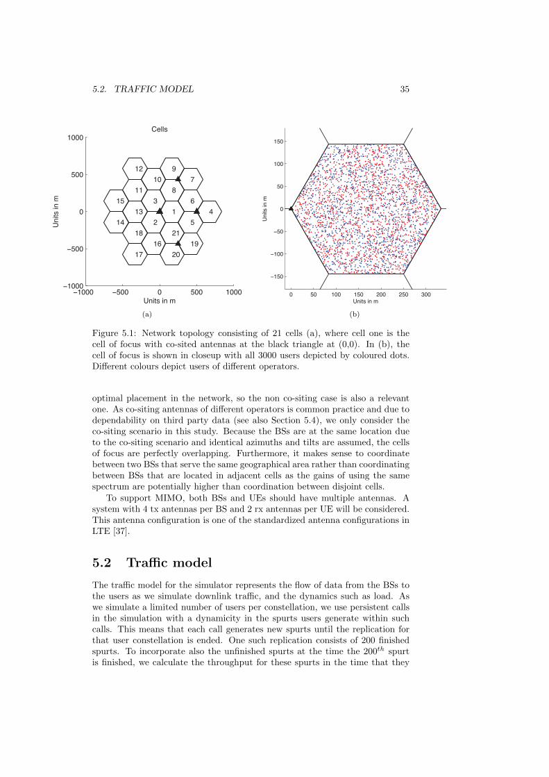
5.2. TRAFFIC MODEL 35
−1000 −500 0 500 1000−1000
−500
0
500
1000
1
2
3
4
5
6
7
8
9
10
11
12
13
14
15
16
17
18
19
20
21
Cells
Units in m
Un
its in
m
(a)
0 50 100 150 200 250 300
−150
−100
−50
0
50
100
150
1
Units in m
Units in m
(b)
Figure 5.1: Network topology consisting of 21 cells (a), where cell one is thecell of focus with co-sited antennas at the black triangle at (0,0). In (b), thecell of focus is shown in closeup with all 3000 users depicted by coloured dots.Different colours depict users of different operators.
optimal placement in the network, so the non co-siting case is also a relevantone. As co-siting antennas of different operators is common practice and due todependability on third party data (see also Section 5.4), we only consider theco-siting scenario in this study. Because the BSs are at the same location dueto the co-siting scenario and identical azimuths and tilts are assumed, the cellsof focus are perfectly overlapping. Furthermore, it makes sense to coordinatebetween two BSs that serve the same geographical area rather than coordinatingbetween BSs that are located in adjacent cells as the gains of using the samespectrum are potentially higher than coordination between disjoint cells.
To support MIMO, both BSs and UEs should have multiple antennas. Asystem with 4 tx antennas per BS and 2 rx antennas per UE will be considered.This antenna configuration is one of the standardized antenna configurations inLTE [37].
5.2 Traffic model
The traffic model for the simulator represents the flow of data from the BSs tothe users as we simulate downlink traffic, and the dynamics such as load. Aswe simulate a limited number of users per constellation, we use persistent callsin the simulation with a dynamicity in the spurts users generate within suchcalls. This means that each call generates new spurts until the replication forthat user constellation is ended. One such replication consists of 200 finishedspurts. To incorporate also the unfinished spurts at the time the 200th spurtis finished, we calculate the throughput for these spurts in the time that they

36 CHAPTER 5. MODELLING
Co-siting Non Co-sitingCo-siting Non Co-siting
Figure 5.2: The difference between co-siting and non co-siting, where operatorsrespectively share a site or are located at disjoint locations.
were active.
Since many users use their devices (phones, laptops) for web surfing, wesimulate web traffic with the simulator. For definition of the distribution ofthe size of web pages, we use data from the HTTP archive [38], a project thatprovides a permanent repository of web performance information such as webpage sizes. The information in this repository is collected by using a browser toaccess a subset of the one million most popular sites according to alexa.com. Notonly does the HTTP archive measure the size of the resulting HTML page, butalso all referenced files like images, JavaScript and css. The database we use inthis report contains data about web pages loaded with a mobile phone, using theMobitest [39] measurement tool. This dataset is more applicable to our scenariocompared to the dataset gathered with a desktop setup, as we simulate mobileusers moving at pedestrian speed. Furthermore, many websites have optimisedversions of their pages for mobile, so the average download size of a web pageis smaller on mobile phones as well. Analysis of the dataset [38] shows that thetotal request size including referenced assets is exponentially distributed witha mean of 561721 bytes. We can use this distribution to calculate the spurtsize for a user when a spurt is generated. Note that another spurt can only begenerated after the previous spurt has been fully downloaded to the UE. As weuse size to define a spurt, the spurt duration is effectively dependent on its sizeand the experienced bit rate.
In-between two downloaded web pages, the user takes some time to read theinformation on the web page. This time is the time between two spurts of oneuser, and can be varied in the simulator to increase or decrease the load. Wecall this time between two spurts the inter-spurt time (Figure 5.3). The longerthe inter-spurt time, the lower the load on the system, and the shorter the inter-spurt time, the higher the load. With an inter-spurt time of zero, each user willimmediately generate a new spurt after finishing its previous one, resulting inthe maximum load the system can be offered with the given model.
The traffic model as described above builds on the traffic models from NextGeneration Mobile Networks (NGMN) and 3rd Generation Partnership Project(3GPP), as described in [40] and [41]. Both models define certain distributionsfor the size of web pages. However, as web page sizes increase fast, calling forrecent measurements, and the NGMN and 3GPP models do not explicitly say
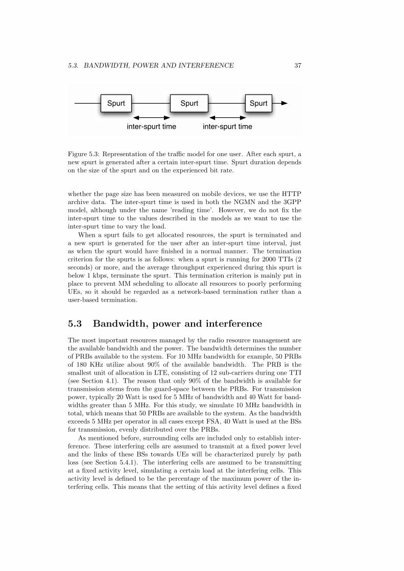
5.3. BANDWIDTH, POWER AND INTERFERENCE 37
Spurt Spurt Spurt
inter-spurt time inter-spurt time
Figure 5.3: Representation of the traffic model for one user. After each spurt, anew spurt is generated after a certain inter-spurt time. Spurt duration dependson the size of the spurt and on the experienced bit rate.
whether the page size has been measured on mobile devices, we use the HTTParchive data. The inter-spurt time is used in both the NGMN and the 3GPPmodel, although under the name ’reading time’. However, we do not fix theinter-spurt time to the values described in the models as we want to use theinter-spurt time to vary the load.
When a spurt fails to get allocated resources, the spurt is terminated anda new spurt is generated for the user after an inter-spurt time interval, justas when the spurt would have finished in a normal manner. The terminationcriterion for the spurts is as follows: when a spurt is running for 2000 TTIs (2seconds) or more, and the average throughput experienced during this spurt isbelow 1 kbps, terminate the spurt. This termination criterion is mainly put inplace to prevent MM scheduling to allocate all resources to poorly performingUEs, so it should be regarded as a network-based termination rather than auser-based termination.
5.3 Bandwidth, power and interference
The most important resources managed by the radio resource management arethe available bandwidth and the power. The bandwidth determines the numberof PRBs available to the system. For 10 MHz bandwidth for example, 50 PRBsof 180 KHz utilize about 90% of the available bandwidth. The PRB is thesmallest unit of allocation in LTE, consisting of 12 sub-carriers during one TTI(see Section 4.1). The reason that only 90% of the bandwidth is available fortransmission stems from the guard-space between the PRBs. For transmissionpower, typically 20 Watt is used for 5 MHz of bandwidth and 40 Watt for band-widths greater than 5 MHz. For this study, we simulate 10 MHz bandwidth intotal, which means that 50 PRBs are available to the system. As the bandwidthexceeds 5 MHz per operator in all cases except FSA, 40 Watt is used at the BSsfor transmission, evenly distributed over the PRBs.
As mentioned before, surrounding cells are included only to establish inter-ference. These interfering cells are assumed to transmit at a fixed power leveland the links of these BSs towards UEs will be characterized purely by pathloss (see Section 5.4.1). The interfering cells are assumed to be transmittingat a fixed activity level, simulating a certain load at the interfering cells. Thisactivity level is defined to be the percentage of the maximum power of the in-terfering cells. This means that the setting of this activity level defines a fixed

38 CHAPTER 5. MODELLING
transmit power with which the interfering cells transmit. The default setting isset at 50%, and another option is an activity level of 30% to study the sensitivityof the performance of the system to interference of the surrounding cells. Themaximum transmission power of the interfering cells is set to be the same asthe BS transmit power in the cell of focus: 40 Watt.
5.4 Physical layer abstraction
As the focus of this study lies in the comparison of the physical layer transmis-sion schemes, as developed by the SAPHYRE project, with other sharing meth-ods, we need input from the project partners to incorporate this into the simu-lator. This way, we can abstract from the physical layer transmission schemesand focus on the scheduling and analysis of the spectrum sharing.
This section serves as a clarification how we get from a propagation model,through the physical layer abstraction, to an actual bit rate for the users. Inthis section, we will introduce the propagation model and the associated chan-nel traces. Furthermore, we will introduce the physical layer traces from thetransmission schemes developed by the SAPHYRE project to get a good under-standing of the data we are dealing with. Subsequently, we will shortly introducethe transmission schemes themselves, as the theory is not an integral part ofthis study, but serves well for further clarification. Finally, we will outline howthe values obtained from the physical layer abstraction are used to calculate anactual bit rate for the users involved.
5.4.1 Propagation model
To know the quality of the channel between transmitter and receiver, we needto know how the signals behave when they travel from the transmitter to thereceiver: the channel response. As mentioned in Chapter 2, the channel re-sponse generally consists of three components: path loss, slow fading and fastfading. For the fast fading component we need channel traces for a numberof TTI and for a certain number of transmit- and receive antennas. The fastfading component of the MIMO channel between a transmitter and receiver isrepresented by a matrix H that defines for n receive- and m transmit anten-nas all possible channel responses between the transmit and receive antennasdenoted by hi,j at time t [42]. Equation 5.2 shows such a channel matrix for2 receive- and 4 transmit antennas, conforming to our model parameters. Fig-ure 5.4 shows a graphical representation of the paths between the transmit- andreceive antennas, as specified by our model parameters.
H(t) =
(h1,1(t) h1,2(t) h1,4(t) h1,4(t)h2,1(t) h2,2(t) h2,3(t) h2,4(t)
)(5.1)
The channel response matrices can be generated by the use of standard-ized models such as SCM, SCME or WINNER (I and II) [42, 43, 37, 44]. Themain difference between the three models is that both WINNER models and theSCME model support larger bandwidth and both WINNER models are appli-cable for more scenarios. All models can theoretically be applied to our system-level simulations because they all provide random delay and angle spreads for
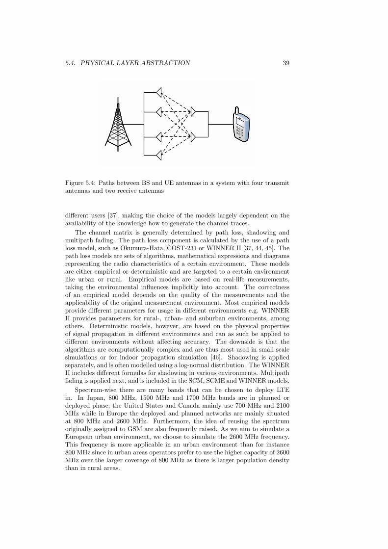
5.4. PHYSICAL LAYER ABSTRACTION 39
Figure 5.4: Paths between BS and UE antennas in a system with four transmitantennas and two receive antennas
different users [37], making the choice of the models largely dependent on theavailability of the knowledge how to generate the channel traces.
The channel matrix is generally determined by path loss, shadowing andmultipath fading. The path loss component is calculated by the use of a pathloss model, such as Okumura-Hata, COST-231 or WINNER II [37, 44, 45]. Thepath loss models are sets of algorithms, mathematical expressions and diagramsrepresenting the radio characteristics of a certain environment. These modelsare either empirical or deterministic and are targeted to a certain environmentlike urban or rural. Empirical models are based on real-life measurements,taking the environmental influences implicitly into account. The correctnessof an empirical model depends on the quality of the measurements and theapplicability of the original measurement environment. Most empirical modelsprovide different parameters for usage in different environments e.g. WINNERII provides parameters for rural-, urban- and suburban environments, amongothers. Deterministic models, however, are based on the physical propertiesof signal propagation in different environments and can as such be applied todifferent environments without affecting accuracy. The downside is that thealgorithms are computationally complex and are thus most used in small scalesimulations or for indoor propagation simulation [46]. Shadowing is appliedseparately, and is often modelled using a log-normal distribution. The WINNERII includes different formulas for shadowing in various environments. Multipathfading is applied next, and is included in the SCM, SCME and WINNER models.
Spectrum-wise there are many bands that can be chosen to deploy LTEin. In Japan, 800 MHz, 1500 MHz and 1700 MHz bands are in planned ordeployed phase; the United States and Canada mainly use 700 MHz and 2100MHz while in Europe the deployed and planned networks are mainly situatedat 800 MHz and 2600 MHz. Furthermore, the idea of reusing the spectrumoriginally assigned to GSM are also frequently raised. As we aim to simulate aEuropean urban environment, we choose to simulate the 2600 MHz frequency.This frequency is more applicable in an urban environment than for instance800 MHz since in urban areas operators prefer to use the higher capacity of 2600MHz over the larger coverage of 800 MHz as there is larger population densitythan in rural areas.
40 CHAPTER 5. MODELLING
The choice of a propagation environment and frequency band limits thechoice of path loss models. The Okumura-Hata and COST-231 path loss modelsare not applicable in this scenario because their frequency range is limited torespectively 50 MHz - 1500 MHz and 1500 MHz - 2000 MHz [47, 48, 49]. For the2600 MHz band, the Stanford University Interim (2500 MHz - 2700 MHz) modelor the WINNER II (2000 MHz - 6000 MHz) path loss model is applicable [44].Both are applicable to urban terrain, but as the WINNER II is more advancedand Fraunhofer-Gesellschaft (FhG) is willing to calculate the channel matricesfor this model, we use this model in our simulations. These channel matrices aregenerated for the parameters of our system model, and this full set of channelmatrices will be referred to as channel traces, as they describe the channel forour users in the modelled time.
As calculation of the channel traces is computationally complex and resourceintensive, we cannot model too many TTIs. The length of the channel tracehas to be chosen carefully as it has to be long enough to be able to see effectsof slow- and fast fading, yet it must not be too long as the data size increaseslinearly with the number of TTIs. Furthermore, this would lead to delay in thedata delivery, surely delaying this study. Therefore, we set the number of TTIsincluded in the channel trace to 1000. This is enough to see effects from slow-and fast fading. As the a replication of the simulation typically takes more thanone second, we can repeatedly loop over the channel traces from front to backand back again to simulate longer timespans.
5.4.2 Physical layer traces
We need to obtain the CSI from BS to UE when we use one of the transmissionschemes schemes to transmit data. This data could for instance be obtained inthe form of a formula which we can apply to the WINNER II channel trace,or in the form of pre-computed traces adapted from the channel trace. As thecalculation in our simulator with a formula turns out to be very computationallycomplex, Linkoping University pre-calculated the traces for the physical layerfor us. These traces serve as input for the simulator, and serves as the inputinformation for the scheduling algorithms.
In the traces of the physical layer, all model aspects have been taken intoaccount to create the experienced SINR values for all the UEs. This includesthe interference from surrounding cells. Like the channel traces provided byFhG, the traces for the physical layer abstraction include SINR values for eachcombination of TTI and PRB. However, the difference between the channeltraces and the traces for the physical layer abstraction is that the latter takethe non-orthogonal usage of the spectrum into account. Instead of one value foreach user, the trace now consists of SINR values for each user for all possiblescheduling combinations. This includes the possibility that no other user isscheduled at the other BS, and the combinations with the users of the other BS.In Table 5.2, we can see the SINR values for one TTI, PRB and user constellationcombination. For users UEA, i and UEB , j where i ∈ {1, 2, . . . , N} and j ∈{1, 2, . . . , N}, we can see the SINRs for both users when the corresponding usersas signified in the first column and row are scheduled together in the currentTTI at the PRB this table signifies. Furthermore, the column and row denotedwith ‘IDLE’ signify the cases where a PRB is just used by one user from oneBS at a time. Note that scheduling for the orthogonal scenarios solely uses this

5.4. PHYSICAL LAYER ABSTRACTION 41
BSB
BSA IDLE UEA,1 UEA,2 · · · UEA,n
IDLE SINRA,1 SINRA,2 · · · SINRA,n
UEB,1 SINRA,1 SINRA,2 · · · SINRA,n
SINRB,1 SINRB,1 SINRB,1 SINRB,1
UEB,2 SINRA,1 SINRA,2 · · · SINRA,n
SINRB,2 SINRB,2 SINRB,2 SINRB,2
......
......
. . ....
UEB,n SINRA,1 SINRA,2 · · · SINRA,n
SINRB,n SINRB,n SINRB,n SINRB,n
Table 5.2: Table for serving one out of n users per BS at a certain TTI at acertain PRB from a certain user constellation
column and row.
5.4.3 Transmission schemes
Linkoping’s Institutionen for Systemteknik (ISY) provides the abstraction layerfor the physical layer transmission schemes so we can evaluate their gain. Tobe sure to keep the input format and the way of calculation of the differentschemes the same, they also provide reference transmission schemes that serveas a reference for evaluation. All schemes are based on game theory, trying tosolve resource conflicts in wireless networks. Game theory falls apart in twocategories: non-cooperative- and cooperative game theory. In non-cooperativegames, players directly compete with each other and cannot strike deals. In co-operative games, however, players can form joint strategies and strike deals witheach other. [50] The supplied transmission schemes used in the simulation con-tain both non-cooperative and cooperative strategies: Nash Equilibrium (NE),Zero-forcing (ZF), Maximum Sum Rate (MSR), Nash Bargaining (NB), andMax-Min (MM).
All the transmission schemes will be described in the next sections. Further-more, the applicability constraints of the schemes are introduced for the formsof spectrum use and coordination between operators.
Nash Equilibrium (NE)
A non-cooperative scheme is supplied with the Nash Equilibrium (NE) trans-mission scheme. The NE solution is a beamforming technique that maximizestransmit diversity. It is also known as maximum-ratio (because it maximizesthe SNR) or as matched-filter (because the SNR maximization is achieved bymatching the direction of the beamforming vector with the one of the channelvector). Since the solution maximizes transmit diversity, the solution gives anupper bound on the gain when compared with LTE’s transmit diversity scheme,and therefore serves as a reference scheme. The NE solution is Pareto optimalfor orthogonal channels. For regular channel realizations however, the NE solu-tion is close to the Pareto boundary for low SNR, but for high SNR the cost ofthe anarchy of a non-cooperative game is unbounded.

42 CHAPTER 5. MODELLING
NE is the reference scheme for LTE and therefore will be used in the FSAscenario. Also, as NE excels with orthogonal spectrum use, we will use thisscheme as well in more dynamic orthogonal sharing. Furthermore, as we areinterested in what will happen when we use the spectrum in a non-orthogonalfashion without coordination between operators, we will also use NE for thatscenario.
Zero-forcing (ZF)
The Zero-forcing (ZF) reference scheme can be considered a cooperative one.The ZF beamformers assure that the transmitter generates no interference onthe other system. To accomplish this, the ZF method requires knowledge of theCSI of the users of the other BSs and thus needs information exchange betweenBSs about CSI of their respective users. The beamforming vector is designedsuch that the interference in the link is cancelled, so it maximizes the numeratorof its own SINR, while minimizing the denominator of the other SINR. The ZFscheme is also considered a reference scheme as this scheme is well-known andwell-described in literature and not developed in the SAPHYRE project.
As ZF requires knowledge of the CSI of the other operator’s users, the ZFis used in a coordinated scenario. Furthermore, because of the nature of thisscheme, the CSI only differs for non-orthogonal cases from the NE scheme.Therefore, this reference scheme is used with non-orthogonal spectrum use.
SAPHYRE schemes
The cooperative schemes are the remaining MSR-, NB- and MM- schemes, de-rived from methods developed in the SAPHYRE project. All these tables dealwith cooperation between BSs to increase the utility of the system. As theschemes are more advanced than the ZF scheme, they are expected to out-perform ZF in the evaluation. It is crucial to understand that a player in acooperative game can be cooperative and rational at the same time. That is,being cooperative does not mean the same thing as being altruistic. Playersmay be willing to accept a bargaining solution that is found to be good enoughfor both when they are interested in maximizing their own outcome. The threetransmission schemes provided each have their own objective: MSR aims tomaximise the sum-rate in the game, NB aims to divide resources in a fair way,and MM aims to maximise the minimum SINR to promote fair throughput.
For usage in different scenarios, the same restrictions apply to these schemesas with ZF. Furthermore, as each transmission scheme has its own objective,we will use the transmission schemes with a scheduling algorithm that matchesin the objective. Herewith, we provide a consistent translation of the operator’sperspective into both the transmission scheme at the physical layer and thescheduling at the Medium Access Control (MAC) layer. We match the MMscheme with MM scheduling because of the similar objective to maximise theminimum rate/SINR. The NB scheme is matched with PF scheduling as theyboth try to divide resources in a fair way, and the MSR scheme is matched withMSR scheduling because of their objectives to maximise the rate/SINR.

5.4. PHYSICAL LAYER ABSTRACTION 43
5.4.4 From abstraction to bit rate
With the traces from the schemes used in the physical layer abstraction, wehave all the input we need to make the scheduling decisions. At the beginningof each new TTI, the simulator calculates the bit rate attained in the last TTIfor each active user, and deducts the transferred bits from the size of their activespurts. To do so, we need to convert the SINR values experienced by the userin the PRBs the user has been assigned into the attained bit rate.
5.4.5 Exponential Effective Signal to Noise Ratio Map-ping (EESM)
The Exponential Effective Signal to Noise Ratio Mapping (EESM) method isused to obtain an effective SINR over a whole transmission, which can be usedto map to a single Modulation and Coding Scheme (MCS), and then to theBLER. EESM is a simple mapping method used when all the PRBs of a userare modulated using the same MCS. The effective SINR (γeff ) is obtained bycombining the SINRs exponentially with the EESM method by performing thefollowing formula:
γeff = EESM(γi, β) = −β ∗ ln(1
N∗
N∑i=1
eγiβ ) (5.2)
In this formula, N denotes the number of PRBs to be averaged, and β isa calibrated value unique to each MCS, obtained from link-level simulationsexecuted by [51, 52, 53, 54].
Adaptive modulation and coding
Now that we have a single SINR, we can employ adaptive modulation and cod-ing (often called link adaptation) to convert the experienced SINR into a singleModulation and Coding Scheme (MCS) for the transmission. The MCS is acombination of a modulation scheme and a code rate. Lower-order modulationis more robust and can tolerate higher levels of interference but provides lowertransmission bit rates. Higher-order modulation offers a higher bit rate, but ismore prone to errors due to higher sensitivity to interference and noise. There-fore, it is only useful when the SINR is sufficiently high. For a given modulation,we can choose the code rate based on the channel conditions: a lower code ratein poor channel conditions and a higher code rate in case of high SINR. Byadapting the modulation and coding techniques used in the communication ata certain PRB, a BS can choose the best MCS for the quality of the channel,rendering better channel utilisation and spectral efficiency [37, 55].
The principle is simple: based on the SINRs experienced in the last TTI,calculate and select a MCS that is optimal for the SINR according to Figure 5.5.The MCSs (numbered 0 to 15) signify different modulation schemes (QPSK,16QAM, 64QAM) with different code rates [37].
Conversion to a bit rate
With the MCS we can look up the MCS- and PRB-specific attainable bit ratein Figure 5.6. To obtain the actually experienced bit rate we need to know the

44 CHAPTER 5. MODELLING
Figure 5.5: Mapping of SINR to MCSs
Block Error Rate (BLER) for the user. The BLER is used to determine successor failure of a certain transmission and is MCS dependent. To assess this BLER,we employ a set of Additive White Gaussian Noise (AWGN) curves as shownin Figure 5.7, derived from link level simulations in which the performance ofdifferent MCSs has been validated [56, 57]. With this BLER, we can flip abiased coin to decide whether the transmission has succeeded or failed. Whenthe transmission succeeds, we can look up the bit rate in Figure 5.6 and convert itto the actual transferred bits. The remaining spurt size is subsequently updatedaccording to the calculated number of transferred bits.

5.4. PHYSICAL LAYER ABSTRACTION 45
Figure 5.6: Mapping of MCS to attainable bit rate. Note that these rates haveto be corrected by ϕD = 0.7788 since not all resources are available for PDSCHbits.
Figure 5.7: BLER, approximated with an 8th degree polynomial

46 CHAPTER 5. MODELLING

Chapter 6
Simulation results &analysis
In Chapter 1, we posed the following question: what can we gain in terms ofperformance and capacity at the system level, by applying the advanced trans-mission schemes for non-orthogonal sharing, as developed in the SAPHYREproject, with respect to Fixed Spectrum Allocation, orthogonal sharing, and non-orthogonal sharing with the ZF transmission scheme? This chapter discussesthe results from the system-level simulations and tries to find answers to theresearch question.
As was stated in the research question we want to know what could be theperformance- and capacity gain of SAPHYRE when compared to other formsof spectrum use and transmission schemes. As a base question this is a validquestion as spectrum is a scarce resource and we can make better use of thisavailable spectrum when we take global scheduling into account. However, it isalso important to know how these techniques behave when we introduce feedbackdelay and error, as was stated in one of the sub questions. Will the system holdits desirable properties (if any)?
To answer these questions, first the simulation scenarios and simulation pa-rameters will be introduced, followed by an overview of the metrics used inanalysis. When the constraints of the simulation and the metrics are set, wewill discuss the differences between the different sharing methods and their as-sociated scheduling algorithms using the simulation results. With a smaller setof desirable scheduling forms, we will perform a sensitivity analysis to see if theperformance degrades when delay and error is introduced.
6.1 Simulation scenarios
In the preceding chapters we wrote about scheduling and spectrum sharing tech-niques. In order to analyse meaningful results, we need to introduce the simula-tion scenarios which we will use for evaluation of the physical layer transmissionschemes. Apart from the modelled parameters, we can distinguish between twovery important factors that determine the simulation scenarios: use of the spec-trum and coordination between BSs. In this section we will provide an overviewof the simulation scenarios that will be used for evaluation of the combinations
47

48 CHAPTER 6. SIMULATION RESULTS & ANALYSIS
of scheduling algorithms and transmission schemes. Figure 6.1 shows the dif-ferent simulation scenarios, clearly categorised in combinations of spectrum useand coordination.
Figure 6.1: Tree of simulation scenarios, scheduling algorithms, and their as-sociated transmission schemes. From the top level of the tree, we first see thedivision between orthogonal and non-orthogonal sharing (pink), followed by adivision of coordination between BSs (orange), and the short name of this sce-nario (red). Working our way down the tree, we see the scheduling algorithms(blue) and their associated transmission schemes (green). Reference transmis-sion schemes are depicted by green circles, SAPHYRE transmission schemes bygreen squares.
The way in which the spectrum is used by the operators is the first main dis-tinction we can identify in classifying the scenarios. As discussed in Chapter 3,we can distinguish between orthogonal and non-orthogonal use of the spectrum.
The second classification aspect of the simulation scenarios is the coordina-tion between BSs. Within uncoordinated scenarios, no communication is neededbetween operators to divide the spectrum or to make scheduling decisions. EachBS manages the spectrum it is allowed to use. Since there is no coordinationbetween the BSs, each BS is only aware of its own users. Consequently onlyscheduling combinations of the operator’s own users are considered, assumingthe other operator does not use the spectrum. Within the coordinated scenar-ios, the CSI of the users of both operators is shared. This enables schedulingon a level that ascends over the individual scheduling decisions of the opera-tors: the system level. Instead of making the scheduling decisions individuallyper operator, the best scheduling combination of the users of both operators is

6.1. SIMULATION SCENARIOS 49
selected by a global scheduler.
Within orthogonal use of the spectrum, the distinction between uncoordi-nated and coordinated scheduling is the distinction where the spectrum is al-located for longer periods to operators (Uncoordinated orthogonal) and wherethe spectrum is allocated to operators more dynamic (Coordinated orthogonal).These two scenarios are extremes within orthogonal spectrum use in how dy-namic the spectrum is allocated. In the uncoordinated orthogonal scenario,which is reminiscent of FSA, each operator is assigned a consecutive 50% of thespectrum, or 25 PRBs. Scheduling decisions are taken by the operator takingonly its own spectrum into account as there is no chance of interference fromother operators. In the coordinated orthogonal scenario, the scheduling deci-sions are made on a global level and the spectrum is assigned to the operatorseach TTI according to the results of the scheduling algorithm for all users ofboth operators. This means that, in case that only one operator has activeusers, all spectrum will be used by this operator. Besides these two extremes inorthogonal spectrum sharing, many mix-forms can be applied like partly fixedspectrum with a dynamic pool for usage by both operators. These mix-formswill not be evaluated.
Within non-orthogonal use of the spectrum, we again differentiate betweentwo extreme forms with regard to coordination. In the uncoordinated non-orthogonal scenario, both operators are allowed to use the whole spectrum,but since there is a lack of coordination, it is possible that they use the samePRBs at the same time. This increases interference and will lead to suboptimalscheduling decisions as we cannot use the SAPHYRE transmission methods dueto the lack of coordination, but are limited to the reference transmission method.In the coordinated non-orthogonal scenario, the scheduling is coordinated on asystem level and either the ZF transmission scheme is used or the SAPHYREtransmission schemes are used. Therefore, the scheduler will take the usersof both operators into account and yield more optimal scheduling decisions.Furthermore, due to the use of advanced transmission schemes, a large partof the interference will be cancelled leading possibly to better rates than theuncoordinated non-orthogonal scenario.
For all four scenarios, we can employ the scheduling algorithms MSR, PF,and MM. However, because the PF algorithm has to deal with two priorityindices per scheduling decision in the coordinated non-orthogonal scenario, forthis scenario we simulate the three different options PFSum, PFProduct, andPFCombi, as described in Chapter 4.
As described in Chapter 5, we can use different transmission schemes totransmit from the BSs to the UEs. Only for the coordinated non-orthogonal sce-nario, we can use the advanced transmission schemes, where ZF is the referencetransmission scheme and NB, MM, and MSR are the SAPHYRE transmissionschemes. The SAPHYRE transmission schemes are used with the schedulingalgorithms that match in goal. For the other scenarios, we use the referencetransmission scheme NE, as the scenarios are either orthogonal or uncoordi-nated.
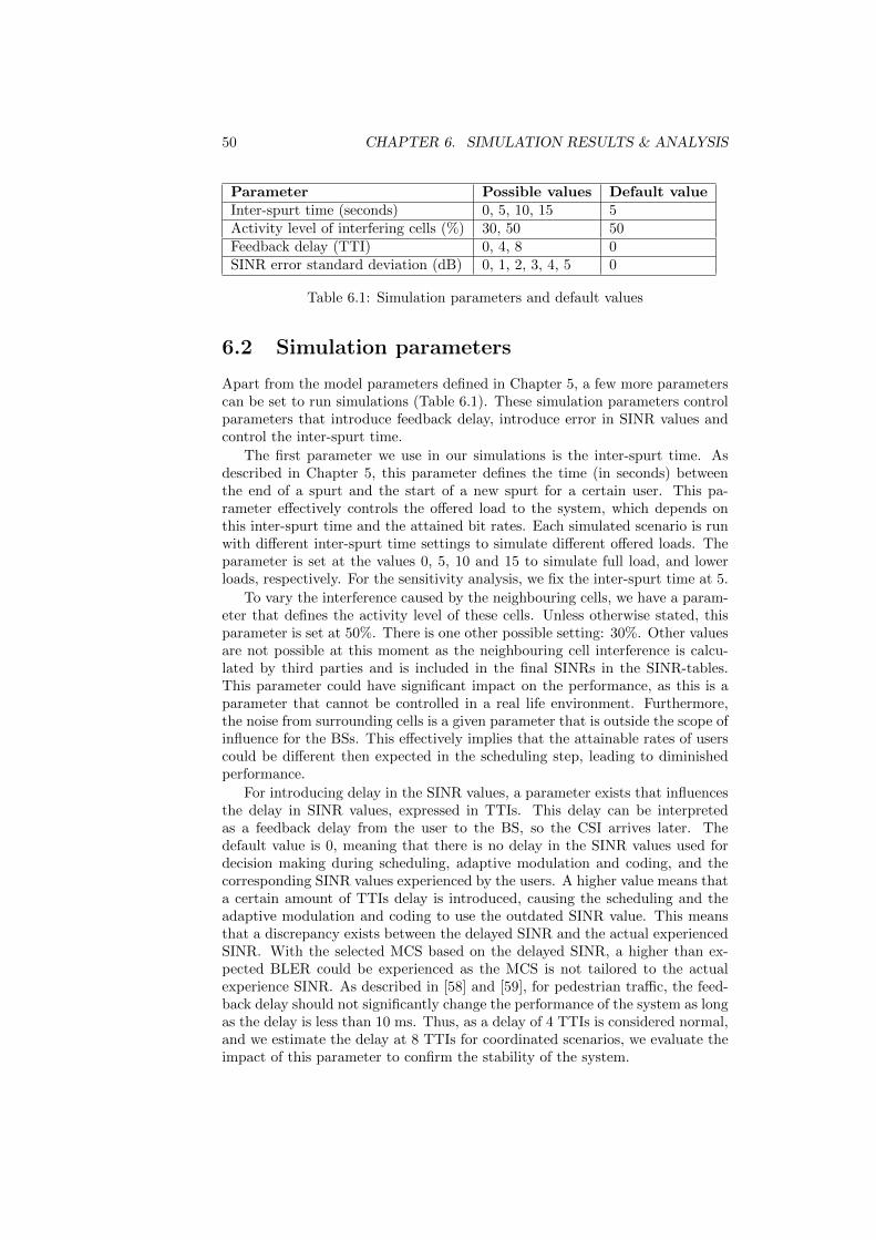
50 CHAPTER 6. SIMULATION RESULTS & ANALYSIS
Parameter Possible values Default valueInter-spurt time (seconds) 0, 5, 10, 15 5Activity level of interfering cells (%) 30, 50 50Feedback delay (TTI) 0, 4, 8 0SINR error standard deviation (dB) 0, 1, 2, 3, 4, 5 0
Table 6.1: Simulation parameters and default values
6.2 Simulation parameters
Apart from the model parameters defined in Chapter 5, a few more parameterscan be set to run simulations (Table 6.1). These simulation parameters controlparameters that introduce feedback delay, introduce error in SINR values andcontrol the inter-spurt time.
The first parameter we use in our simulations is the inter-spurt time. Asdescribed in Chapter 5, this parameter defines the time (in seconds) betweenthe end of a spurt and the start of a new spurt for a certain user. This pa-rameter effectively controls the offered load to the system, which depends onthis inter-spurt time and the attained bit rates. Each simulated scenario is runwith different inter-spurt time settings to simulate different offered loads. Theparameter is set at the values 0, 5, 10 and 15 to simulate full load, and lowerloads, respectively. For the sensitivity analysis, we fix the inter-spurt time at 5.
To vary the interference caused by the neighbouring cells, we have a param-eter that defines the activity level of these cells. Unless otherwise stated, thisparameter is set at 50%. There is one other possible setting: 30%. Other valuesare not possible at this moment as the neighbouring cell interference is calcu-lated by third parties and is included in the final SINRs in the SINR-tables.This parameter could have significant impact on the performance, as this is aparameter that cannot be controlled in a real life environment. Furthermore,the noise from surrounding cells is a given parameter that is outside the scope ofinfluence for the BSs. This effectively implies that the attainable rates of userscould be different then expected in the scheduling step, leading to diminishedperformance.
For introducing delay in the SINR values, a parameter exists that influencesthe delay in SINR values, expressed in TTIs. This delay can be interpretedas a feedback delay from the user to the BS, so the CSI arrives later. Thedefault value is 0, meaning that there is no delay in the SINR values used fordecision making during scheduling, adaptive modulation and coding, and thecorresponding SINR values experienced by the users. A higher value means thata certain amount of TTIs delay is introduced, causing the scheduling and theadaptive modulation and coding to use the outdated SINR value. This meansthat a discrepancy exists between the delayed SINR and the actual experiencedSINR. With the selected MCS based on the delayed SINR, a higher than ex-pected BLER could be experienced as the MCS is not tailored to the actualexperience SINR. As described in [58] and [59], for pedestrian traffic, the feed-back delay should not significantly change the performance of the system as longas the delay is less than 10 ms. Thus, as a delay of 4 TTIs is considered normal,and we estimate the delay at 8 TTIs for coordinated scenarios, we evaluate theimpact of this parameter to confirm the stability of the system.
6.3. OVERVIEW OF METRICS 51
Another parameter is defined for the error in the SINR values: the standarddeviation (in dB). This parameters defines the Gaussian error applied to theSINR values used for scheduling, and can be regarded as a channel estimationerror. The default value is 0, meaning that there is no error in the SINR. As withthe delay parameter, the error only affects scheduling and adaptive modulationand coding. The mean value of the SINR error is always 0, so it is possiblefor the system to either over- or underestimate the SINR during scheduling.As we can observe from [60], the performance of mobile networks will decreasewith increasing error in the channel estimation. The reason for diminishedperformance is quite straightforward: by introducing error in the values onwhich the scheduling is based, the scheduling algorithm will not be able tomake the most optimal scheduling combination, reducing system performance.
6.3 Overview of metrics
To evaluate the performance of the system in the various scenarios and to beable to compare these scenarios, we define the following metrics which will beintroduced in this section:
• Offered load;
• Average PRB utilisation;
• Average UE throughput;
• Average UE throughput by distance from the BS;
• 10th percentile UE throughput;
• Fairness.
An important system-level metric is the offered load. The offered load is definedas the total number of bits offered to the system divided by the simulated time.This metric depends on inter-spurt time, as a higher inter-spurt time meansthat less load is offered to the system and thus less throughput will be reached.Note that the offered load is similar to the system throughput as users cannotstart a new spurt before the last one ended. Therefore, the system can never beoverloaded, meaning that the maximum system throughput is reached with aninter-spurt time of 0. This metric will be useful in comparison of the capacityof the different sharing techniques and scheduling algorithms. With full load(inter-spurt time of 0), we can see the theoretical upper bound for the systemthroughput with all scheduling choices as all users keep receiving data. Withlower offered loads, we can see how different scheduling algorithms perform whenwe cannot necessarily make the best combinations (in terms of the schedulinggoal) of scheduled users as less users are available simultaneously. The offeredload is an average of the offered load in all the 150 replications.
A metric that is closely related to the load is the average PRB utilisation.This metric signifies the average PRB usage from the perspective of the BSs.With full load, it gives an indication whether the scheduling algorithm makesefficient use of the available spectrum as a value less than 100% would meannot all PRBs are used in each TTI. With decreasing load, it gives an idea ofthe share of time the channel is unused as the scheduling algorithms will always

52 CHAPTER 6. SIMULATION RESULTS & ANALYSIS
try to fully utilize the available spectrum. For orthogonal sharing scenarios,it is expected that the maximum PRB utilisation is 50%, as only half of thespectrum will be used by each operator.
The average UE throughput is a user-centred metric signifying the averagethroughput over all users. In order to compute this average throughput, the totaltransferred bits of all spurts of a user are divided by the sum of the transmissiontime of the spurts. Note that this translates into a weighted average over allspurts of a user since we take the transmission times into account. To generatethe average UE throughput metric, these user throughput for all 3000 users (150replications times 20 users) are averaged.
Not only are we interested in the average UE throughput over the wholesystem, but also analysed over distance between the user and the BS. As, onaverage, the channel quality should be better near the BS than far away, weexpect this measure to decrease over distance. In order to provide this metric,we categorize the users into ten distance zones from the BS. As the maximumdistance is 300 meters, each zone is 30 meters wide. The reason to categorizethe distance from the BS is to make sure that enough users are evaluated for acertain range of distance to get a representative average throughput.
Closely related to the average UE throughput, we calculate a CumulativeDistribution Function (CDF) of user throughput. In the analysis we use the10th percentile, to give an idea of the minimum rates achieved. This metricmeans that 90% of the users has experienced a minimum average throughputof the depicted rate. As such, we can easily see if the user experience wouldbe acceptable for the majority of users. The higher the 10th percentile rate,the better the experience for the users. The 10th percentile user throughputis generated by taking the average throughputs of all users and generating theCDF from that data.
A metric that is important for the user, but even more important for theoperator is the fairness of the user throughput. As a user you would want tohave a certain quality of service even when you are located on the cell edge,and as an operator you would want to promote fairness between users becausethese users have these quality of service constraints. To quantify fairness, wehave to realise that the even allocation of the user throughput over all users isdeemed fair. The more uneven this allocation is, the more unfair the scheme. Tocalculate the fairness, we use Jain’s fairness index [61]. Jain’s fairness index is ametric calculating fairness over a set of metrics (x1, x2, . . . , xn), see Equation 6.1.In our case, we use the user throughputs as input for the calculation. Thefairness index is bounded between 0 and 1, and can as such be interpreted as apercentage. A value of 0.1 means that the scheme is unfair to 90% of the users,whereas a value of 0.9 means that the scheme is unfair to only 10% of the users.In general, a higher fairness index means that the user throughputs are moreevenly distributed over all users.
J(x1, x2, . . . , xn) =(∑ni=1 xi)
2
n ∗∑ni=1 x
2i
(6.1)
6.4. SPECTRUM SHARING ANALYSIS 53
6.4 Spectrum sharing analysis
According to Figure 6.1, we have in total 19 leaves at the tree, which meansthat 19 distinct sets of simulations have been executed to form the basis of theanalysis in this section. For each of the 19 combinations, we simulated accordingto the default simulation parameters (Table 6.1), including all options for theinter-spurt time. In this section, we take a look at the performance of these 19combinations of spectrum use, scheduling algorithms and transmission schemes.To prevent confusing graphs due to the number of schemes, the simulationshave been grouped by the different scenarios. The results of the simulations aredepicted in Figure 6.2 until Figure 6.5.
6.4.1 Uncoordinated orthogonal sharing (FSA)
One of the reference scenarios, FSA, is the scenario depicting how the spectrumis used nowadays (Figure 6.2a - 6.2f). In our simulations each operator ownsa consecutive part of 50% of the spectrum. The operators do not have to dealwith interference from other operators on their share of the spectrum as thespectrum is used orthogonally. The physical layer scheme used is NE, as this isan uncoordinated scheme that gives an upper bound to using transmit diversity.
Figure 6.2f shows the offered load on the vertical axis, with varying inter-spurt times on the horizontal axis. As we can see, the maximum load thesystem can cope with is just over 30 Mbps in the case of MSR scheduling. ThePF algorithm performs worse than MSR with about 24 Mbps under full load,and the MM algorithm can only handle just shy of 20 Mbps of traffic. As weincrease the inter-spurt time, the offered load decreases. With increasing inter-spurt times the algorithms approach one another in offered load, indicatingthat the algorithms can all transmit the surplus in load that differentiated themfrom each other in the 0 inter-spurt time case within the inter-spurt times of theother users. Furthermore, there might even be time that the BSs are idle, i.e.do not have active user spurts. However, the MM scheduling algorithm remainsthe worst in terms of offered load even with longer inter-spurt times, suggestingthat the MM algorithm is inefficient in scheduling even under lower system load.As the objective of the MM scheduling algorithm is to maximise the minimumrate, the scheduling algorithm will often prefer users with lower bit-rates overusers with higher bit-rates to increase the rates of the former. The effect is thatthe spectrum is used less efficient than with MSR and PF, which both also takethe system throughput into account.
As expected, we can confirm that BSs have more idle time in Figure 6.2d.In this figure, the average PRB utilisation is shown for the offered loads as inFigure 6.2f. For full system load, all algorithms reach 50% PRB usage, whichis expected as each operator can only use its own share of the spectrum inthe uncoordinated orthogonal scenario. For lower loads, the PRB utilisationdecreases as the system fails to use all PRB as it is waiting certain amounts oftime for new spurts to arrive due to the inter-spurt times.
As for the 10th percentile throughput and the average user throughput (Fig-ure 6.2a and 6.2b), we can observe that the MSR algorithm assures highestaverage throughput and MM the lowest, but the 10th percentile throughput isdominated by the PF algorithm. It deserves notice that the 10th percentilethroughput for full load in the MSR algorithm is 0.0, meaning that at least 10%

54 CHAPTER 6. SIMULATION RESULTS & ANALYSIS
of the users experience no throughput at all. This is due to the fact that MSRalways schedules the best users, and since each user generates new spurts in-stantly, users with lower attainable bit rates do not get a chance to be scheduled.This improves with longer inter-spurt times as users with less favourable channelconditions are scheduled in-between spurts of users with more favourable con-ditions. As said, MM performs the worst in the average user throughput. Forthe 10th percentile throughput, it is a bit more complicated. When we trans-late the data points in the graph to inter-spurt times, we can see by lookingat Figure 6.2f that the data points are in decreasing order for inter-spurt time.This means that the rightmost data points signify the maximum load that thealgorithms can cope with. Therefore, we can say that the MM algorithm actu-ally dominates the MSR algorithm for full load as the MM algorithm manages0.25 Mbps 10th percentile UE throughput, where the MSR algorithm managesto offer nothing to these users. However, as the load decreases, we can see thatfor all other inter-spurt times the MM algorithm is on par, or below the otheralgorithms making it still the worst performing algorithm in this scenario.
Fairness-wise, we can clearly see in Figure 6.2c that the PF algorithm dom-inates in terms of fairness between users. The higher the load, the better thePF algorithm can provide fairness between users, up until over 80%. The MMalgorithm follows suit with a marginally smaller at full load, and a somewhatbigger gap at the lowest load. Both the PF and the MM algorithm have curvesthat increase with increasing offered load. This is due to the fact that bothalgorithms will equalize the rates more when more users are available. Withlower loads, it is possible that only one user is active at a time, yielding him themaximum rate as he will be assigned all PRBs. For the MSR algorithm, theoverall curve is contrary to the other algorithms. When the system experiencesfull load, the fairness is low due to the tendency to only serve the very bestusers for the same reasons outlined before. With lower offered loads, users thatwould not be served with full load can be served in-between the spurts of higherperforming users, thus increasing fairness as they will actually be allowed toreceive data instead of being ignored by the scheduling algorithm due to badchannels. Note that the MSR algorithm will never be more fair than the PFand MM algorithm, as in the case when only one user has an active transmis-sion at a time, the fairness will be equal for all algorithms. In cases with moreactive users however, the MSR algorithm will choose the best performing user,decreasing fairness.
Figure 6.2e shows the average user throughput over distance from the BS.The graph shows the throughput with an inter-spurt-time of five seconds. Asexpected, this follows a clear downward trend with increasing distance from theBS for the MSR algorithm. This clearly indicates that users closer to the BS onaverage have better channel conditions. For PF and MM, the downward trendis less pronounced as the fairness of these schemes is higher, meaning that UEsfar away (with also get a chance to receive data) will get more attention by thealgorithm.
6.4.2 Uncoordinated non-orthogonal sharing
Figure 6.3a - 6.3f show similar graphs as we just analysed, for non-orthogonaluncoordinated sharing of the spectrum. As discussed earlier, in this scheme BSscan use the whole spectrum and select users regardless of the choice of the other

6.4. SPECTRUM SHARING ANALYSIS 55
Legend
MSR NE PFSum NE MaxMin NE
0 10 20 30 40 50 60 70Offered load [Mbps]
0.0
0.5
1.0
1.5
2.0
2.5
3.0
10th percentile UE throughput [Mbps]
(a) 10th percentile UE throughput vs offered load
0 10 20 30 40 50 60 70Offered load [Mbps]
0
2
4
6
8
10
12
Average UE throughput [M
bps]
(b) Average UE throughput vs offered load
0 10 20 30 40 50 60 70Offered load [Mbps]
0.0
0.2
0.4
0.6
0.8
1.0
Jain's Fairness index
(c) Jain’s Fairness index vs offered load
0 10 20 30 40 50 60 70Offered load [Mbps]
0
20
40
60
80
100
Average PRB utilisation [per BS] (%
of total 50 PRB)
(d) PRB utilisation vs load
0 50 100 150 200 250 300Distance [meters]
0
5
10
15
20
Average UE throughput [M
bps]
(e) Average UE throughput vs distance (at 5 seconds inter-spurttime)
0 2 4 6 8 10 12 14Inter-spurt time [seconds]
0
10
20
30
40
50
60
70
Offered load [Mbps]
(f) System throughput vs inter-spurt time
Figure 6.2: Graphs for different aspects of uncoordinated orthogonal sharing(FSA).

56 CHAPTER 6. SIMULATION RESULTS & ANALYSIS
BS. This means that the expectation of the channel quality during schedulingdoes not align with the experienced channel quality due to added interferenceof users scheduled on the same PRBs from the other BS.
The offered load generated with the varying inter-spurt-times is about twothirds of the load generated with the uncoordinated orthogonal scheme for MSR,and a less drastic decrease for the PF and MM algorithms. The lower offeredload at an inter-spurt time of 0 is likely to be caused by overestimation of thechannel due to the added interference by the other BS transmitting on thesame spectrum. This means that the BLER will be higher due to lower SINR,effectively increasing the error rate due to the choice of a wrong MCS. Atlower inter-spurt times however, the offered load is similar to the load in theuncoordinated orthogonal sharing, suggesting that this scenario is capable ofhandling the same loads when the system is not fully loaded.
The PRB usage is 100% at full load as expected since each BS can use thewhole spectrum. With lower load, we see the PRB usage decrease indicating anidle channel at times. The PRB usage drop of the MM algorithm is less than theother algorithms, which can be explained by the lower average user throughputof this algorithm due to the increased fairness. This lower throughput impliesthat the transfers of spurts are longer in duration, leading to higher PRB usageas the idle time is less.
For the average user throughput, this sharing method is overall worse thanuncoordinated orthogonal sharing with MSR scheduling. For both PF and MMscheduling, the average user throughput is similar at higher loads, but higher atlower loads. The 10th percentile UE throughput is overall higher for all schemes,but also has the highest gain at lower loads, just as the average throughput forPF and MM scheduling. A reason for this observation is that the total numberof PRBs available is bigger, resulting (in the fair scheduling algorithms) in moreassigned PRBs for users with lower channel qualities, which corrects for thediminished SINR due to added interference. Because MSR focuses on the bestperforming users, the drop in average user throughput is higher than with theother algorithms, as a user with higher attainable decreases relatively more inthroughput than a user that would already have had a lower rate. With lowerloads the system has more available bandwidth, and if no concurrent users atthe other BS are scheduled, the bit rates will be higher across the board due tothe ability to schedule more PRBs.
Over distance, the order of the different algorithms remains the same (MSRthe best and MM the worst). However, the average throughputs are spacedmore closely together. Notably, MM virtually has the same throughput overdistance as in the FSA scheme. The tails of the throughput over distance creepmore together, and at the edge of the cell, the MSR algorithm is even ever soslightly worse than the PF algorithm.
6.4.3 Coordinated orthogonal sharing
Coordinated orthogonal sharing (Figure 6.4a - 6.4f) is similar to uncoordinatedorthogonal sharing in terms of the spectrum sharing: the spectrum is used inan orthogonal fashion. However, the BSs do not have their own fixed piece ofspectrum, but the spectrum is coordinated in usage and shared in full betweenboth BSs. The scheduling algorithms decide which PRB is assigned to whichuser on a system level and thus effectively also assigns the spectrum to the

6.4. SPECTRUM SHARING ANALYSIS 57
Legend
MSR NE PFSum NE MaxMin NE
0 10 20 30 40 50 60 70Offered load [Mbps]
0.0
0.5
1.0
1.5
2.0
2.5
3.0
10th percentile UE throughput [Mbps]
(a) 10th percentile UE throughput vs offered load
0 10 20 30 40 50 60 70Offered load [Mbps]
0
2
4
6
8
10
12
Average UE throughput [M
bps]
(b) Average UE throughput vs offered load
0 10 20 30 40 50 60 70Offered load [Mbps]
0.0
0.2
0.4
0.6
0.8
1.0
Jain's Fairness index
(c) Jain’s Fairness index vs offered load
0 10 20 30 40 50 60 70Offered load [Mbps]
0
20
40
60
80
100
Average PRB utilisation [per BS] (%
of total 50 PRB)
(d) PRB utilisation vs offered load
0 50 100 150 200 250 300Distance [meters]
0
5
10
15
20
Average UE throughput [M
bps]
(e) Average UE throughput vs distance (at 5 seconds inter-spurttime)
0 2 4 6 8 10 12 14Inter-spurt time [seconds]
0
10
20
30
40
50
60
70
Offered load [Mbps]
(f) Offered load vs inter-spurt time
Figure 6.3: Graphs for different aspects of uncoordinated non-orthogonal shar-ing.

58 CHAPTER 6. SIMULATION RESULTS & ANALYSIS
operators. As the spectrum is used orthogonally, we can not take advantage ofthe desirable properties of the SAPHYRE schemes as there is no interference onthe channel generated by other users. However, as the SINR of NE is the sameas SAPHYRE for orthogonal cases, this is a baseline in what the coordinatedSAPHYRE schemes can provide when used orthogonally.
When we look at the offered load generated with different inter-spurt-times,we can see that the curves look almost like a replica of the same graph for theuncoordinated orthogonal scenario. The scenario does introduce more flexibilityin scheduling as the whole spectrum is usable when only one operator has activeusers, which can be confirmed with the average UE throughput and the 10th
percentile throughput. In both the average UE throughput and the 10th per-centile throughput, we can observe overall higher throughputs for lower loadsin PF and MSR scheduling. For maximum load the average user throughputand 10th percentile throughput remains the same, which is an effect of that theusers keep generating spurts, and the maximum capacity of scheduling over 50PRBs is the same as scheduling over two times 25 PRBs. The MM schedulingalgorithm does not gain as much from the coordination as the other schedulingalgorithms do, as the scheduling algorithm now takes all users from both opera-tors into account. This means that if one lower performing user is active in thesystem, all users will see lower rates as the system tries to maximise the rate ofthe lower performing user. Therefore, instead of only affecting the users of oneBS, this now affects users of all BSs.
Higher average UE throughputs with similar offered load should translateto higher PRB usage, which is indeed the case for the MSR and PF schedulingalgorithm. For MM, the PRB usage is lower on average for lower load, which isan effect of the decreased average UE throughput at lower load due to the factthat the scheduling takes place for the whole system and thus the slowest userin the system slows down the other users as well.
From the fairness graph, we can observe that PF and MSR are a little bitless fair, and MM slightly more fair for non-maximum loads compared to theuncoordinated orthogonal scenario. The latter can be explained as the MM nowslows down the whole system instead of just the users of one BS when there isa slower user present, yielding a higher fairness as the rates over all users aremore equal, and the former can be explained by the observation that the averagerates are higher due to the possibility to exploit more PRBs for scheduling.
6.4.4 Coordinated non-orthogonal sharing
Lastly, we consider the coordinated non-orthogonal scenario, in which the schedul-ing is executed on a system level and the spectrum is used non-orthogonally.Besides the simulation of the advanced physical layer transmission schemes fromthe SAPHYRE project, we also simulate the ZF transmission scheme, a beam-forming scheme that can be considered a reference scheme. The SAPHYREschemes are expected to outperform the ZF transmission scheme, as outlined be-fore. Furthermore, because of the specific challenges of non-orthogonal schedul-ing, we evaluate all three PF algorithms: PFSum, PFProduct and PFCombi.The results of the coordinated non-orthogonal scenario can be seen in Figure 6.5a- 6.5f.
When we look at the offered load, we can observe an almost twofold increaseof the maximum load (with 0 inter-spurt time) when compared to the orthog-
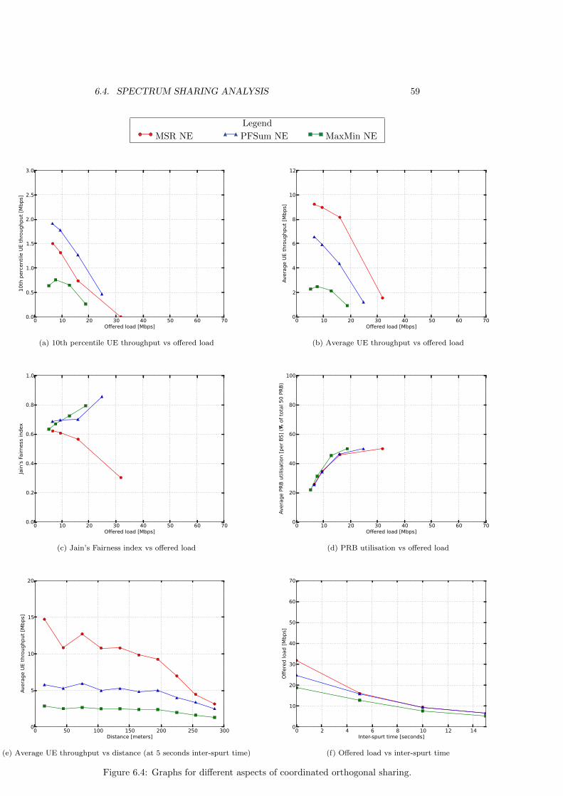
6.4. SPECTRUM SHARING ANALYSIS 59
Legend
MSR NE PFSum NE MaxMin NE
0 10 20 30 40 50 60 70Offered load [Mbps]
0.0
0.5
1.0
1.5
2.0
2.5
3.0
10th percentile UE throughput [Mbps]
(a) 10th percentile UE throughput vs offered load
0 10 20 30 40 50 60 70Offered load [Mbps]
0
2
4
6
8
10
12
Average UE throughput [M
bps]
(b) Average UE throughput vs offered load
0 10 20 30 40 50 60 70Offered load [Mbps]
0.0
0.2
0.4
0.6
0.8
1.0
Jain's Fairness index
(c) Jain’s Fairness index vs offered load
0 10 20 30 40 50 60 70Offered load [Mbps]
0
20
40
60
80
100
Average PRB utilisation [per BS] (%
of total 50 PRB)
(d) PRB utilisation vs offered load
0 50 100 150 200 250 300Distance [meters]
0
5
10
15
20
Average UE throughput [M
bps]
(e) Average UE throughput vs distance (at 5 seconds inter-spurt time)
0 2 4 6 8 10 12 14Inter-spurt time [seconds]
0
10
20
30
40
50
60
70
Offered load [Mbps]
(f) Offered load vs inter-spurt time
Figure 6.4: Graphs for different aspects of coordinated orthogonal sharing.
60 CHAPTER 6. SIMULATION RESULTS & ANALYSIS
onal scenarios. For the lower offered loads due to a longer inter-spurt time,we can see that the coordinated non-orthogonal scenario sustains only slightlyhigher offered load than the orthogonal scenarios. This observation leads usto believe that most of the gain in throughput in this scheme is coming fromthe scheduling of combinations of two users at one PRB, combined with theinterference cancellation in the transmission schemes. With longer inter-spurttimes, the number of combinations we can make between active users duringscheduling becomes less, making it less likely to schedule a good combinationof users. Furthermore, when increasing the inter-spurt time even higher, thecoordinated non-orthogonal scenario will behave the same as the coordinatedorthogonal scenario as in most cases only one user will be active in the systemdue to the long inter-spurt times, forcing the system to schedule orthogonally.For the inter-spurt times of 5 and 10 seconds, we can still see a marginal increaseover the coordinated orthogonal scheme as apparently sometimes the system canmake good combinations of scheduled users.
Globally, the offered load for the different scheduling algorithms behaves sim-ilar as in the other scenarios, but we can see here that the elaborate PFProductand PFCombi algorithms for PF scheduling perform significantly worse than thesimple PFSum algorithm. In the PRB usage graph, we can see that at full loadonly 50% of the PRBs is used per BS for PFProduct and PFCombi scheduling,indicating that the bad performance stems from the way in which the priorityindices are combined. In fact, both PFProduct and PFCombi scheduling al-gorithms seem to use the spectrum orthogonally in the majority of schedulingcases. This can be caused by users that have a priority index of in fact are alwayslower than the priority index of an orthogonally scheduled user, reducing theglobal scheme to an orthogonal scheme. As the performance of these schedulingalgorithms is now essentially the same as PF in coordinated orthogonal sharing,we will not discuss these scheduling algorithms further here.
The expectation that the SAPHYRE transmission schemes would outper-form ZF cannot be observed from the graphs. In fact, the MM transmissionscheme with MM scheduling even performs significantly worse than ZF withMM scheduling. This can be explained by the fact that the MM transmissionscheme specifically tries to equalize the SINR for the users by performing smartbeamforming, resulting in lower SINR for the user with better channel qualityin the ZF transmission scheme and marginally higher SINR for the weaker users.For the other transmission schemes, the curves for all graphs are similar if notalmost the same. The observation that the MSR and PF scheduling algorithmshave similar performance under both ZF and SAPHYRE transmission schemescan be explained because the interference of the other user is quite high, andeffectively nulled out by both algorithms. However, the SAPHYRE schemesare also applicable in other scenarios like when each BS serves multiple usersper PRB by spatial multiplexing. The interference situation will then changedrastically, and the SAPHYRE schemes will probably outperform ZF in thatscenario. Also, in this light a non co-sited scenario might as well show im-provement. Furthermore, the SAPHYRE schemes might perform better in thisscenario with less users, as described in [2].
Both the average UE throughputs and the 10th percentile throughputs areconsistently higher than all other scenarios evaluated. Combined with a slightlyhigher system throughput at longer inter-spurt times, this means that the usershave consistently better rates due to the non-orthogonal use of the spectrum

6.4. SPECTRUM SHARING ANALYSIS 61
and the coordinated scheduling. This in turn means that spurts of comparablesize are downloaded to the UE faster, providing a better user experience.
In Figure 6.5c, we can see the fairness of the different combinations ofscheduling algorithm and transmission scheme in the coordinated non-orthogonalscenario. Because we work with more scheduling algorithms in this scenario, andall scheduling algorithms are evaluated for two transmission schemes, the graphis a bit crowded in the 60% to 80% area. Therefore, we included an enlargementof this part in Figure 6.6. We can immediately see that, although the MM al-gorithm with the MM transmission scheme performs worst in the average userthroughput and offered load metrics, it performs stronger than MM with theZF transmission scheme in fairness. In fact, when we look at the fairness ofMM scheduling with MM transmission, than it seems to be more in line withthe fairness in other scenarios for MM scheduling than with the ZF transmis-sion scheme. Again, this is caused by the optimization in the MM transmissionscheme that tries to equalize the SINR of the scheduled users, leading to bet-ter fairness between users. Another observation is that both the PFCombi andPFProduct scheduling algorithms perform best in fairness with 85% althoughthey in fact schedule more orthogonally and perform bad in the other metrics.
6.4.5 Sharing scenario comparison
Now that we have evaluated the various sharing scenarios with respect to themetrics, we can compare these sharing scenarios with each other. From a sce-nario perspective, we can see that the coordinated non-orthogonal scenario hasthe best performance across the board. This comes however at the cost of coor-dination between operators, so we will analyse the sensitivity to the delay causedby this coordination later in this report. Furthermore, the coordinated orthog-onal scenario shows promise over the uncoordinated orthogonal scenario in av-erage user throughput and 10th percentile throughput. As the uncoordinatednon-orthogonal scenario performs worst, we cannot say that non-orthogonalspectrum sharing alone is the holy grail for the imminent spectrum crunch.However, it can be a solution when combined with coordination between oper-ators. In this section we will compare the different scenarios for each metric.
Offered load
The offered load metric is an important metric to compare the schemes witheach other. Due to the design of the system, this metric can be directly relatedto the system throughput, and with an inter-spurt time of 0, we can show thetheoretical upper limit of the system throughput.
As we have observed before, only in the simulations with an inter-spurt timeof 0 the offered load really differs in the different sharing scenarios. With higherinter-spurt times, the load becomes more or less the same for all scenarios, al-though the coordinated non-orthogonal scenario consistently reaches a little bitmore load. The convergence of the offered load at higher inter-spurt times iscaused by the fact that the inter-spurt times are multiples of the transmissiontime for most users. As this is the case, marginal average speed differences donot show in the offered load metric. For 0 inter-spurt time however, all usersdirectly generate new spurts after finishing the previous spurt, so we can seethe maximum maintainable system throughput. When the load is maximised,
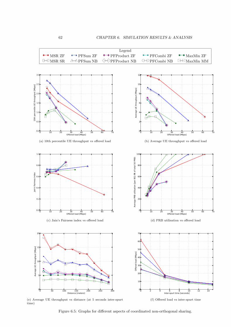
62 CHAPTER 6. SIMULATION RESULTS & ANALYSIS
Legend
MSR ZF PFSum ZF PFProduct ZF PFCombi ZF MaxMin ZF
MSR SR PFSum NB PFProduct NB PFCombi NB MaxMin MM
0 10 20 30 40 50 60 70Offered load [Mbps]
0.0
0.5
1.0
1.5
2.0
2.5
3.0
10th percentile UE throughput [Mbps]
(a) 10th percentile UE throughput vs offered load
0 10 20 30 40 50 60 70Offered load [Mbps]
0
2
4
6
8
10
12
Average UE throughput [M
bps]
(b) Average UE throughput vs offered load
0 10 20 30 40 50 60 70Offered load [Mbps]
0.0
0.2
0.4
0.6
0.8
1.0
Jain's Fairness index
(c) Jain’s Fairness index vs offered load
0 10 20 30 40 50 60 70Offered load [Mbps]
0
20
40
60
80
100
Average PRB utilisation [per BS] (%
of total 50 PRB)
(d) PRB utilisation vs offered load
0 50 100 150 200 250 300Distance [meters]
0
5
10
15
20
Average UE throughput [M
bps]
(e) Average UE throughput vs distance (at 5 seconds inter-spurttime)
0 2 4 6 8 10 12 14Inter-spurt time [seconds]
0
10
20
30
40
50
60
70
Offered load [Mbps]
(f) Offered load vs inter-spurt time
Figure 6.5: Graphs for different aspects of coordinated non-orthogonal sharing.
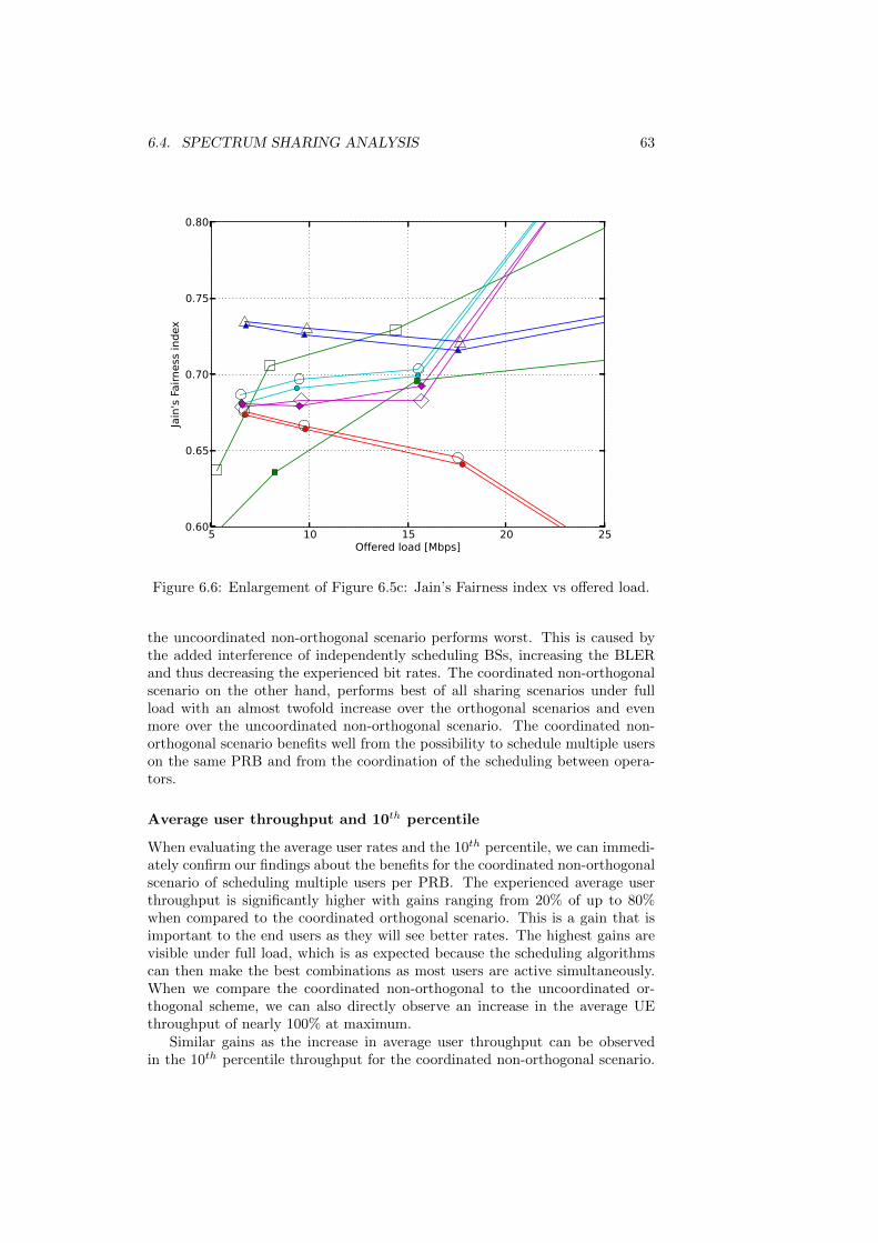
6.4. SPECTRUM SHARING ANALYSIS 63
5 10 15 20 25Offered load [Mbps]
0.60
0.65
0.70
0.75
0.80
Jain's Fairness index
Figure 6.6: Enlargement of Figure 6.5c: Jain’s Fairness index vs offered load.
the uncoordinated non-orthogonal scenario performs worst. This is caused bythe added interference of independently scheduling BSs, increasing the BLERand thus decreasing the experienced bit rates. The coordinated non-orthogonalscenario on the other hand, performs best of all sharing scenarios under fullload with an almost twofold increase over the orthogonal scenarios and evenmore over the uncoordinated non-orthogonal scenario. The coordinated non-orthogonal scenario benefits well from the possibility to schedule multiple userson the same PRB and from the coordination of the scheduling between opera-tors.
Average user throughput and 10th percentile
When evaluating the average user rates and the 10th percentile, we can immedi-ately confirm our findings about the benefits for the coordinated non-orthogonalscenario of scheduling multiple users per PRB. The experienced average userthroughput is significantly higher with gains ranging from 20% of up to 80%when compared to the coordinated orthogonal scenario. This is a gain that isimportant to the end users as they will see better rates. The highest gains arevisible under full load, which is as expected because the scheduling algorithmscan then make the best combinations as most users are active simultaneously.When we compare the coordinated non-orthogonal to the uncoordinated or-thogonal scheme, we can also directly observe an increase in the average UEthroughput of nearly 100% at maximum.
Similar gains as the increase in average user throughput can be observedin the 10th percentile throughput for the coordinated non-orthogonal scenario.

64 CHAPTER 6. SIMULATION RESULTS & ANALYSIS
For full load however, the MSR algorithm does not show an increase in 10th
percentile throughput as the algorithm will also in this scenario choose theusers with the best channel quality.
An important observation from the average UE throughput over distance isthat the curves of the better performing scenarios are steeper than the curvesof the scenarios that perform worse. However, the average UE throughput atthe cell edge is also increased, so not all of the performance gain we see in theaverage UE throughput comes at the expense of users at the cell edge.
Fairness
Fairness-wise, the general trend of the PF and MM algorithms is that theybecome more fair towards users when the system has more offered load. Thisis due to the fact that the scheduling algorithms are able to choose betweendifferent users when multiple users are active simultaneously. With lower loadshowever, it is less common that multiple users are active, so the algorithmscannot do anything different than allocating as much spectrum as possible. Thismeans that the fairness will become similar to the fairness in attainable bit ratesbetween users in extreme low loads. The MSR algorithm follows a downwardstrend as the algorithm allocates most of its PRBs to users with good channelquality when multiple users are active. This means some users will get little orno PRBs assigned, leaving an unfair distribution of the resources.
PRB usage
The main difference in PRB usage is the difference between non-orthogonal andorthogonal sharing, where the BSs will on average use either maximum 50%or 100%, respectively. With maximum offered load, all scenarios reach theirmaximum PRB usage, but PFCombi and PFProduct in the coordinated non-orthogonal scenario. The reason for the lower PRB usage with the PFCombiand PFProduct algorithm is that the way in which the priority indices are com-bined in these algorithms seems to promote orthogonal scheduling combinations,although the scenario enables non-orthogonal combinations as well. With loweroffered loads, the PRB usage decreases in all scenarios as the BSs are idle fora certain amount of time due to times when no active users are available forscheduling.
6.4.6 Scheduling algorithm comparison
From an operator’s perspective user experience is a very important issue. Ifyou consistently provide bad user experience, your clients will eventually findanother operator as the playing field is very competitive.
Overall, for systems which are not under full load, the MSR algorithm per-forms best. The PF algorithm does provide a better overall experience as thisalgorithm provides better bit rates when the system is fully loaded and is notthe worst performer in the rest of the cases. MM can be regarded as the weak-est scheme, as the fairness is not that much better than PF, and the trade-offin average user throughput is quite dramatic as well as the trade-off in systemthroughput. Furthermore, MM is the most complex algorithm, making the MM

6.4. SPECTRUM SHARING ANALYSIS 65
algorithm even less favourable. Because of the desirable properties of both PF-Sum and MSR, we select these scheduling algorithms for sensitivity analysis tosee how the algorithms perform under less favourable conditions.
Of the three forms of PF scheduling algorithms, we already shortly analysedthat the PFSum algorithm was the best. This is mainly due to the fact thatboth PFProduct and PFCombi make almost orthogonally use of the spectrum,leaving no room for the gains we can get from non-orthogonal sharing. Thisreduces the algorithms to the same performance as the PFSum algorithm inthe coordinated orthogonal scenario. This leads to the conclusion that the wayin which the two priority indices of the users are combined in PFProduct andPFCombi are suboptimal, leading to lower priority indices than the orthogonaldecision would.
In the remainder of this section, the different scheduling algorithms will becompared with regards to the various metrics.
Offered load
In terms of offered load, the MSR scheduling algorithm consistently providesthe highest offered load, indicating that it can handle the most traffic. Thisis quite logical when we remember that the objective of MSR scheduling isto maximize the sum-rate of the system. Yet, this high throughput is onlyreached with higher system loads. With lower loads it eventually decreases tothe throughput of PF scheduling. The lowest system throughput is consistentlygenerated by the MM scheduling algorithm, as this algorithm will give a fairamount of attention to users with bad channel conditions.
Average user throughput and 10th percentile
The average user throughput shows the same order of the scheduling algorithmsas does the offered load metric; the MSR scheduling algorithm reaches the high-est average user throughput. This also remains true with lower offered loads,suggesting a higher spread of experienced average user throughput than the PFor MM algorithm. Indeed, in the 10th percentile throughput graphs, we canobserve that this larger spread is the case as the PF (PFSum for the coordi-nated non-orthogonal scenario) takes the lead in this metric. Furthermore, 10%of the users actually experience a rate of zero when the system is fully loadedwith MSR scheduling, indicating that the MSR scheduling algorithm takes itsobjective very seriously at the expense of users experiencing bad channel quality.
With even longer inter-spurt times than we simulated, the average rates forthe non-orthogonal scenarios will likely decrease to the coordinated orthogonalscenario as scheduling combinations become scarce when less users are activesimultaneously. We can see this effect already with MM in the coordinatednon-orthogonal scenario. Furthermore, PF and MSR already show signs ofstabilization of the average user throughput with lower loads. Although MSRprovides higher average rates, from an operator’s perspective the PF algorithmis better for the user experience when the system gets fully loaded.
Fairness
Fairness-wise, the MM and PF algorithms both score similarly with increasingfairness when the load increases and between 60% up to almost 90% fairness.

66 CHAPTER 6. SIMULATION RESULTS & ANALYSIS
0 5 10 15 20 25 30UE throughput [Mbps]
0
20
40
60
80
100
Percentile
(a) CDF for an inter-spurt time of 0
0 5 10 15 20 25 30 35UE throughput [Mbps]
0
20
40
60
80
100
Percentile
(b) CDF for an inter-spurt time of 5
Figure 6.7: Cumulative Distribution Function (CDF) of UE throughput for theMSR scheduling algorithm in the coordinated non-orthogonal scenario
MM seems to flourish with uncoordinated non-orthogonal sharing, in which itreaches its top fairness. For the other scenarios, the PF algorithm takes thelead. The MSR scheduling algorithm is less fair with its fairness ranging from25% under full load up to 65% under lower loads. The low fairness of MSRscheduling under full load makes you wonder how many users actually experiencezero bit rate. Figure 6.7a shows the CDF for MSR scheduling under full load inthe coordinated non-orthogonal scenario. As can be observed from this graph,around 40% of the users experience zero bit rate and 75% of the users experiencemaximum 5 Mbps on average, making the MSR algorithm quite unsuitable foroperators when they experience full load. For reference, Figure 6.7b shows theCDF of user throughput for an inter-spurt time of 5. We can observe from thisgraph that the average UE throughput is spread more even over the users. Incontrast to the other scheduling algorithms, with the MSR algorithm fairnessincreases under lower loads. This can be explained by the fact that the userswith high rates will be served fast, and the users with lower rates can be servedin-between these high-performing users, which is not possible under full load asthe high performing users keep being active. As the MSR algorithm does notdeserve a ‘fair’ predicate, this round is a tie between PF and MM scheduling.However, we need to remember that MSR fairness increases radically when thesystem is not fully loaded.
6.5 Sensitivity analysis (coordinated non-orthogonalsharing)
In this section we analyse the sensitivity of the PFSum and the MSR schedulingalgorithm in the coordinated non-orthogonal scenario, with respect to interfer-ence, error in the SINRs and feedback delay. To get a fair comparison, we
6.5. SENSITIVITY ANALYSIS (COORDINATEDNON-ORTHOGONAL SHARING)67
consider one deviating parameter from the default values at a time, with allother parameters kept equal. This ceteris paribus assumption rules out the pos-sibility that other factors influence the observed effects, and allows us to focuson the sensitivity to one varying parameter at a time. Because redoing all thesimulations for all inter-spurt times would be very time-sensitive, we choose tosimulate with an inter-spurt time of five seconds, as this is the lowest settingwhere the system throughput of the different algorithms is similar. Further pa-rameters are kept at their default values as described earlier in this Chapter. Asthe error, delay and interference could likely have some impact on the spreadof measured values, we include a 95% confidence interval in all graphs for thesensitivity analysis.
We are mainly interested in the sensitivity of the transmission schemes in thecoordinated non-orthogonal scenario, as this includes the transmission schemesdeveloped by the SAPHYRE project. Furthermore, as we argued before, thecoordinated non-orthogonal scenario is the best performing scenario. For thescheduling algorithms we choose to evaluate the MSR and the PFSum algorithmas they are the best performing algorithms in all scenarios.
6.5.1 Sensitivity to interference of surrounding cells
To analyse the effect of interference of surrounding cells on the system, extrainput data from the SAPHYRE partners is needed as the interference is in-cluded in the traces for the transmission schemes. The default parameter of theinterference generated by the surrounding cells is based on an activity level of50%. Due to the constraints of the input data, we only have one other option atour disposal: an activity level of 30%. Figure 6.8 shows the results of the sim-ulations with an activity level of 30% and the corresponding simulations withthe default setting of 50%.
As can be observed from Figure 6.8a, the total offered load increases onlymarginally with lowered interference. As the 95% confidence interval over-lap partly with both interference activity levels, we cannot be sure that themarginally lower offered load, we cannot be confident that the effect is causedby the change of the interference level or just by the specific simulation. If theincrease is caused by the interference level, we should be able to see an increasein the average user throughput as well.
Figure 6.8b confirms the increased average user throughput with quite somedifference between the levels of interference. We can observe from the averageuser throughput graph that the PFSum algorithm has more gain (about 15%)than the MSR algorithm (about 8%). An explanation for this effect can be thatthe MSR algorithm already focuses on scheduling the users with the highestattainable bit rates. Users that would already would have had the highest MCSin the default scenario will not see a bit rate increase. Therefore, these userswith high bit rates are still the most likely to be scheduled. Only the users withlower bit rates see the real advantage of the lowered interference. In the PFSumalgorithm, users with lower bit rates in the default scenario gain more from theincreased SINRs as their increased attainable bit rates increases their priorityindices making it more likely that they are scheduled.
Figure 6.8c shows with the 10th percentile user throughput that the reductionin interference is beneficial to all users in the system. For MSR this is valid aswell, because the increased bit rates of the users makes more room for users
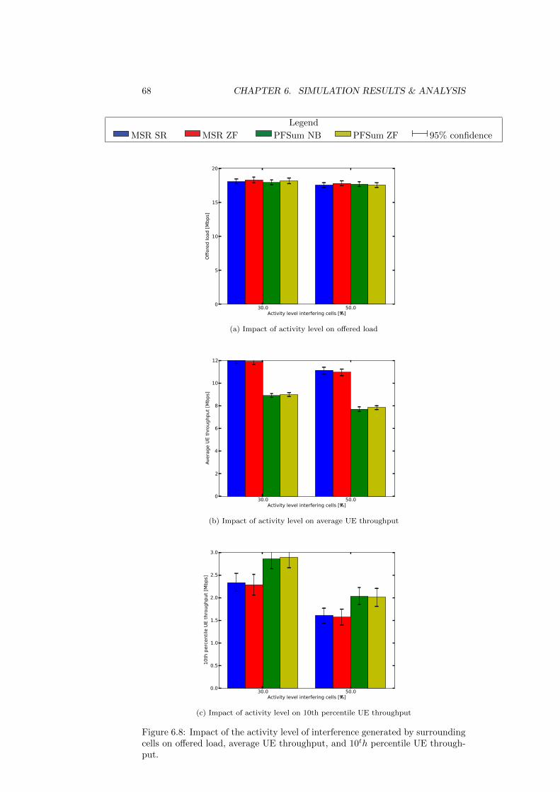
68 CHAPTER 6. SIMULATION RESULTS & ANALYSIS
Legend
MSR SR MSR ZF PFSum NB PFSum ZF 95% confidence
30.0 50.0Activity level interfering cells [%]
0
5
10
15
20
Offered load [Mbps]
(a) Impact of activity level on offered load
30.0 50.0Activity level interfering cells [%]
0
2
4
6
8
10
12
Average UE throughput [Mbps]
(b) Impact of activity level on average UE throughput
30.0 50.0Activity level interfering cells [%]
0.0
0.5
1.0
1.5
2.0
2.5
3.0
10th percentile UE throughput [M
bps]
(c) Impact of activity level on 10th percentile UE throughput
Figure 6.8: Impact of the activity level of interference generated by surroundingcells on offered load, average UE throughput, and 10th percentile UE through-put.
6.5. SENSITIVITY ANALYSIS (COORDINATEDNON-ORTHOGONAL SHARING)69
with smaller bit rates as all spurts are finished faster. In the PFSum algorithm,the increase in 10th percentile throughput stems from the fact that users withlower attainable bit rates will have more chance to be scheduled due to theirincreased bit rates when compared to the default scenario.
6.5.2 Sensitivity to feedback delay
The effects of introducing a 4- and 8-TTI delay in the SINRs used for schedulingare displayed in Figure 6.9. As can be observed from these graphs, the differencebetween no delay and 4- or 8-TTI delay is negligible. As explained before, this isas expected as the users move at pedestrian speed and thus the channel qualitychanges only marginally within this time window. As the results are very closeand within each others 95% confidence intervals, we cannot observe any trend.This leads us to the conclusion that a 4- to 8-TTI delay in the channel qualitydoes not impact users moving at pedestrian speed. However, as is mentioned in[59], pedestrian users should be able to tolerate up to a 10-TTI delay withoutsignificant impact. It might therefore be a good idea to test this assumption ina follow-up study by simulating even longer delays.
6.5.3 Sensitivity to feedback error
For the SINR error, we introduced three different values of the error. The error issampled from a Gaussian distribution with a standard deviation of 1 dB, 2 dB, 3dB, 4 dB or 5 dB and a mean of 0 dB. Figure 6.10 shows the effect of introducingthe error in the SINRs. As the SINR error has a mean of 0 dB, the SINR canboth be underestimated or overestimated with each scheduling decision for eachcombination of users. This means that, in the case of underestimation, thechannel quality of the user will be better than expected during scheduling andMCS selection, and in case of overestimation, the rate of the user will be worsethan expected. Selecting the wrong MCS for a certain channel quality causesthe BLER to be higher when the channel quality is overestimated, leading tolower bit rates. When the channel quality is underestimated however, the BLERis lower resulting in a good transmission, though possibly a better MCS couldhave been chosen that would have increased the bit rate. Furthermore, dueto working with uncertain data in the scheduling, the scheduling algorithmslikely make suboptimal decisions in the scheduling combinations, leading tolower throughputs. Due to these concerns, we expect that the performance ofthe system in both user throughput and total offered load will decrease withincreasing error.
Looking at the offered load (Figure 6.10a), a decrease is clearly visible witherrors of 3 dB and higher. With 1 dB and 2 dB of error, the total offered loadis similar to the default of 0 dB error. A slight downwards trend seems visible,but because the 95% confidence intervals are overlapping, purely based on thatdata we cannot be certain of a decrease. With 3 dB, 4dB and 5 dB error,a downwards trend in offered load begins speeding up. With 5 dB error, theoffered load is only 60% for PF scheduling, and 68% for MSR. Such a decreasein the offered load means that the it takes the users significantly longer to finishtheir spurts.
We can confirm that the average spurt will take longer to complete by lookingat the average user throughput (Figure 6.10b). We can observe the same trend

70 CHAPTER 6. SIMULATION RESULTS & ANALYSIS
Legend
MSR SR MSR ZF PFSum NB PFSum ZF 95% confidence
0.0 4.0 8.0SINR delay [TTI]
0
5
10
15
20
Offered load [Mbps]
(a) Impact of delay on offered load
0.0 4.0 8.0SINR delay [TTI]
0
2
4
6
8
10
12
Average UE throughput [M
bps]
(b) Impact of delay on average UE throughput
0.0 4.0 8.0SINR delay [TTI]
0.0
0.5
1.0
1.5
2.0
2.5
3.0
10th percentile U
E throughput [M
bps]
(c) Impact of delay on 10th percentile UE throughput
Figure 6.9: Impact of feedback delay on offered load, average UE throughput,and 10th percentile UE throughput.

6.5. SENSITIVITY ANALYSIS (COORDINATEDNON-ORTHOGONAL SHARING)71
Legend
MSR SR MSR ZF PFSum NB PFSum ZF 95% confidence
0.0 1.0 2.0 3.0 4.0 5.0SINR error standard deviation [dB]
0
5
10
15
20
Offered load [Mbps]
(a) Impact of SINR error on offered load
0.0 1.0 2.0 3.0 4.0 5.0SINR error standard deviation [dB]
0
2
4
6
8
10
12
Average U
E throughput [M
bps]
(b) Impact of SINR error on average UE throughput
0.0 1.0 2.0 3.0 4.0 5.0SINR error standard deviation [dB]
0.0
0.5
1.0
1.5
2.0
2.5
3.0
10th
perc
entile
UE thro
ughput [M
bps]
(c) Impact of SINR error on 10th percentile UE throughput
Figure 6.10: Impact of feedback error on offered load, average UE throughput,and 10th percentile UE throughput.

72 CHAPTER 6. SIMULATION RESULTS & ANALYSIS
as in the offered load with the real decrease beginning at an error of 3 dB.However, in this graph, we can also observe that the PF algorithm starts itsdescent already clearly at an error of 2 dB.
The 10th percentile throughput (Figure 6.10c) shows again the same down-wards curve as the the average user throughput. In the 10th percentile through-put however, we can observe that the PF algorithm performs higher than theMSR algorithm with 0 dB and 1 dB error; it performs similar at an error of 2dB, and worse than MSR at errors of 3 dB and higher. Due to this effect andthe increased rate of decrease for PF in the other metrics, we can say that theMSR algorithm is more resilient to SINR error than the PF algorithm. Thiscan be explained by the focus of the MSR algorithm at users with good channelquality. The high channel quality users in a scenario with error will most of thetime still be users in the higher channel quality regions that either overestimatedtheir channel quality to unrealistically high values or have underestimated a lit-tle, causing a higher BLER but on a high bit rate as well. So the remainingbit rate might be higher than a user in the lower channel quality regions thatthe PF algorithm is more likely to serve, that have overestimated their channelquality to the point where they can actually receive data but in reality are belowthe threshold for any successful data transfer. Furthermore, a higher BLER onlower bit rates in effect still means even lower experienced bit rates. So thefocus on the higher channel quality users of the MSR algorithm is the qualitythat makes it more resilient to SINR error.
Taking all the metrics into account, we can conclude that the MSR algorithmis more tolerant to smaller SINR error than the PF algorithm. The MSR algo-rithm will not see significant impact on offered load, average user throughputand 10th percentile throughput for errors of 1 dB or 2 dB, while the PF algo-rithm only tolerates a 1 dB error before decreasing significantly in the averageuser throughput and the 10th percentile user throughput.

Chapter 7
Conclusions and futurework
This thesis quantified the performance of different scenarios of spectrum use ona system level including model parameters that reflect a realistic environment.In this chapter, we conclude this thesis with general conclusions about the re-sults and analysis presented in the preceding chapter. Furthermore, we presentrecommendations for future work.
7.1 Conclusions
The transmission schemes developed by the SAPHYRE project have been eval-uated at link-level assessments, lacking realistic aspects of network operationlike scheduling, feedback delay, multi-user traffic, propagation environmentsand network layout. To provide a realistic system-level simulation, we mod-elled a realistic urban environment with WINNER II empirical channel traces,two co-sited operators and 3000 users, homogeneously spread over the cell anddivided in 150 groups of 20 randomly selected users which are active simulta-neously. We introduced a traffic model consisting of multiple spurts per userwith an exponentially distributed inter-spurt time, and the size of the spurtsdistributed as the empirical website size data as found in the HTTP archivegathered with mobile phones. Furthermore, we described a physical layer ab-straction and used it in the simulator to incorporate the transmission schemesof the SAPHYRE project as well as the NE transmission scheme serving as areference for LTE and the ZF transmission scheme serving as a reference fornon-orthogonal spectrum sharing. Furthermore, we described the MSR, PFand MM scheduling algorithms and suggested a way to deal with schedulingin a coordinated non-orthogonal scenario because scheduling two users on thesame resource is a significantly different problem from scheduling only one user.For PF scheduling this led to three possible scheduling algorithms: PFSum,PFCombi and PFProduct.
In order to assess the results of the spectrum sharing scenario simulations,we analysed the metrics regarding the load offered to the system, the averageuser throughput, the 10th percentile user throughput, fairness, and PRB usage.Based on this analysis, we selected the coordinated non-orthogonal scenario with
73
74 CHAPTER 7. CONCLUSIONS AND FUTURE WORK
PFSum and MSR scheduling for sensitivity analysis to analyse how the systemholds under feedback delay, feedback error, and interference of surrounding cells.
7.1.1 Answer to the research questions
In the introduction of this thesis, we established the following research question:what can we gain in terms of performance and capacity at the system level, byapplying the advanced transmission schemes for non-orthogonal sharing, as de-veloped in the SAPHYRE project, with respect to Fixed Spectrum Allocation, or-thogonal sharing, and non-orthogonal sharing with the ZF transmission scheme?In order to answer this research question, we break it up into three separatequestions:
• What can we gain with respect to uncoordinated orthogonal sharing (FSA)?
• What can we gain with respect to coordinated orthogonal sharing?
• What can we gain with respect to coordinated non-orthogonal sharingwith the ZF transmission scheme?
First, we will focus on above questions, followed by a focus on the sensitivityof the SAPHYRE scheme to feedback delay, feedback error and interference ofsurrounding cells.
SAPHYRE gain
When we compare the SAPHYRE transmission schemes in the coordinated non-orthogonal scenario with uncoordinated orthogonal sharing, we can immediatelyobserve an improvement across the board. Not only can the operators use thewhole spectrum in the coordinated non-orthogonal scenario, but they can alsouse it at the same time (with coordinated scheduling between the operators).When we look at both scenarios under full load, we can observe an almosttwofold increase in offered load and average user throughput for all schedulingalgorithms. This comes at a small cost in fairness for both PFSum and MSRscheduling. At lower loads the offered load to the system converges to the unco-ordinated orthogonal scenario. However, the almost twofold increase in averageuser throughput remains. For the 10th percentile user throughput it deservesmention that the MSR scheduling algorithm does not increase its metric withthe SAPHYRE transmission schemes at full load, but does at lower loads, likethe PFSum algorithm. The PFProduct and PFCombi scheduling algorithm per-form similar to the PFSum algorithm in the uncoordinated orthogonal scenarioin offered load albeit with a little bit higher average user throughput and 10th
percentile user throughput.Compared to the coordinated orthogonal scenario, the SAPHYRE transmis-
sion schemes in the coordinated non-orthogonal scenario also show improvement.The coordinated orthogonal scenario extends the uncoordinated orthogonal sce-nario with coordination between operators, and thus with the ability to use thewhole spectrum instead of only their own spectrum share in a coordinated fash-ion. As it is still an orthogonal scheme, the maximum offered load does notchange, so the situation remains the same: an almost twofold increase for theSAPHYRE transmission schemes. However, the ability to coordinate the spec-trum usage between operators has its effect on the average user throughput and

7.1. CONCLUSIONS 75
the 10th percentile throughput in comparison with uncoordinated orthogonal,as operators are allowed to use 100% of the spectrum when the other opera-tor has no active users. Therefore, the gain in average user throughput and10th percentile throughput is less dramatic between the SAPHYRE transmis-sion schemes in the coordinated non-orthogonal scenario and the coordinatedorthogonal scenario than above comparison with the uncoordinated orthogonalscenario. At full load, the increase is almost twofold in average user throughput,but at lower loads the gain decreases to around 35%.
The last comparison is between the SAPHYRE transmission schemes and theZF transmission scheme, both in the coordinated non-orthogonal scenario. Al-though the SAPHYRE transmission schemes are expected to outperform theZF transmission scheme, the performance of both is very similar if not al-most the same for the MSR, PFSum, PFProduct, PFCombi, and MM schedul-ing algorithms. Only the MM algorithm with the SAPHYRE transmissionscheme (MM) shows consistently worse performance than the MM algorithmwith the ZF transmission scheme. The similar performance between the ZFand SAPHYRE transmission schemes might be caused by, as suggested bySAPHYRE project partners, the co-sited setup of the scenario. Furthermore,when more than one user per PRB per operator is served, the interference sit-uation will change dramatically, likely giving the SAPHYRE schemes betterperformance than the ZF transmission scheme.
Sensitivity
For sensitivity analysis, we selected the MSR and the PFSum scheduling algo-rithm to evaluate the sensitivity of the SAPHYRE schemes to feedback delay,feedback error and interference of surrounding cells. Furthermore, for compari-son we included the ZF transmission scheme to see how the SAPHYRE schemesstack up to this transmission scheme in suboptimal conditions.
The interference level of surrounding cells (expressed in an activity percent-age) does not have a significant effect on the offered load to the system whencomparing between 30% and 50% interference. However, with a higher interfer-ence level, the average user throughput drops by 15% for the PFSum algorithmand by 8% for the MSR algorithm. In the 10th percentile throughput we canobserve a drop as well, with the PFSum algorithm again taking a higher dropthan the MSR algorithm.
The effect of feedback delay on the average user throughput, 10th percentileuser throughput and offered load is negligible for a 4- or 8-TTI delay. This ismainly caused by the fact that we simulate pedestrian users with low speed,which are suggested in literature to tolerate a delay of up to 10 TTIs. However,for coordinated spectrum sharing an 8-TTI delay seems enough to account fordelays in LTE (4 TTIs) and delays in coordination (another 4 TTIs).
The effect of feedback error in the SINR values has a somewhat larger im-pact on the system. An error of 1 dB is manageable by both the MSR andthe PFSum algorithm, but with 2 dB the PFSum algorithm begins decreasingaverage user throughput and 10th percentile user throughput. The MSR algo-rithm is stable under errors up to 2 dB and therefore a little bit more resilientto the error than the PFSum algorithm. With an error of 5 dB, the PFSumalgorithm takes an almost 40% decrease in offered load, where the MSR algo-rithm takes a smaller decrease of 32%. The average user throughput decreases
76 CHAPTER 7. CONCLUSIONS AND FUTURE WORK
by around 50% for the PFSum algorithm and 45% for the MSR algorithm. The10th percentile throughput really suffers with a meagre less than 0.1 Mbps 10th
percentile throughput left for both scheduling algorithms.The MSR scheduling algorithm is slightly more resilient in the sensitivity
analysis. However, this comes at the cost of selecting only the best performingusers to be scheduled, which is disastrous for the 10th percentile user through-put under full load, as we have demonstrated before. No observable differencescan be found between the ZF transmission scheme and the SAPHYRE trans-mission schemes in sensitivity to feedback delay, feedback error and interferenceof surrounding cells.
7.2 Future work
Whilst working on this thesis, it was suggested by the SAPHYRE project part-ners that the gain of the SAPHYRE schemes might be even higher when notusing a co-sited scenario. Furthermore, serving even more than one user perPRB per operator might also drastically change the interference, giving theSAPHYRE schemes a gain over the ZF transmission scheme. In this light, werecommend to run simulations for the non co-sited scenario as well to verify thisclaim. Furthermore, we recommend extending the simulator to provide a way ofsimulating multiple users per PRB per operator. With minor modifications, thePFSum, MSR and MM scheduling algorithm will work with this new extension.
Furthermore, we recommend to also investigate a more generic way to anal-yse the effects of spectrum sharing. For instance, this could be a generic algo-rithm that generates SINR values instead of the complex physical layer abstrac-tion for which we need third party input. This generic process could be usedto quantify results regarding questions relating to the impact of the realisticaspects of a system-level simulator on for instance an average increase of SINRvalues of 3 dB.

Bibliography
[1] M. Haardt, Z. K. M. Ho, E. Jorswieck, E. Karipidis, J. Kibilda, J. Li,J. Lindblom, C. Scheunert, J. Sykora, D. Gesbert, E. G. Larsson, andJ. Zhang, “Adaptive and robust signal processing in multi-user and multi-cellular environments (initial) D3.1a,” tech. rep., SAPHYRE, 2011.
[2] T. Yoo and A. Goldsmith, “On the optimality of multiantenna broadcastscheduling using zero-forcing beamforming,” IEEE Journal on Selected Ar-eas in Communications, vol. 24, pp. 528 – 541, March 2006.
[3] J. Belrose, “Reginald Aubrey Fessenden and the birth of wireless tele-phony,” IEEE Antennas and Propagation Magazine, vol. 44, pp. 38 –47,April 2002.
[4] J. Cimini, L., “Analysis and simulation of a digital mobile channel us-ing Orthogonal Frequency Division Multiplexing,” IEEE Transactions onCommunications, vol. 33, pp. 665 – 675, July 1985.
[5] M. Pereirasamy, J. Luo, M. Dillinger, and C. Hartmann, “Dynamic inter-operator spectrum sharing for UMTS FDD with displaced cellular net-works,” in IEEE Wireless Communications and Networking Conference,2005, vol. 3, pp. 1720 – 1725, March 2005.
[6] M. Buddhikot, “Understanding dynamic spectrum access: Mod-els,taxonomy and challenges,” in 2nd IEEE International Symposium onNew Frontiers in Dynamic Spectrum Access Networks, 2007. DySPAN2007, pp. 649 –663, April 2007.
[7] Q. Zhao and B. Sadler, “A survey of dynamic spectrum access,” IEEESignal Processing Magazine, vol. 24, pp. 79 –89, May 2007.
[8] D. Hatfield and P. Weiser, “Property rights in spectrum: taking the nextstep,” in First IEEE International Symposium on New Frontiers in Dy-namic Spectrum Access Networks, 2005. DySPAN 2005, pp. 43 –55, Novem-ber 2005.
[9] W. Lehr and J. Crowcroft, “Managing shared access to a spectrum com-mons,” in First IEEE International Symposium on New Frontiers in Dy-namic Spectrum Access Networks, 2005. DySPAN 2005, pp. 420 –444,November 2005.
77

78 BIBLIOGRAPHY
[10] P. Leaves, K. Moessner, R. Tafazolli, D. Grandblaise, D. Bourse, R. Tonjes,and M. Breveglieri, “Dynamic spectrum allocation in composite reconfig-urable wireless networks,” IEEE Communications Magazine, vol. 42, pp. 72– 81, May 2004.
[11] T. Yamada, D. Burgkhardt, I. Cosovic, and F. K. Jondral, “Resource dis-tribution approaches in spectrum sharing systems,” EURASIP Journal onWireless Communications and Networking, 2008.
[12] I. Mitola, J., “Cognitive radio for flexible mobile multimedia communica-tions,” in IEEE International Workshop on Mobile Multimedia Communi-cations, 1999. MoMuC 1999, pp. 3 –10, 1999.
[13] Q. Zhao and A. Swami, “A survey of dynamic spectrum access: Signalprocessing and networking perspectives,” in IEEE International Conferenceon Acoustics, Speech and Signal Processing, 2007. ICASSP 2007, vol. 4,pp. 1349–1352, April 2007.
[14] T. Weiss and F. Jondral, “Spectrum pooling: an innovative strategy forthe enhancement of spectrum efficiency,” IEEE Communications Magazine,vol. 42, pp. 8–14, March 2004.
[15] E. Jorswieck, L. Badia, T. Fahldieck, D. Gesbert, S. Gustafsson, M. Haardt,K.-M. Ho, E. Karipidis, A. Kortke, E. Larsson, H. Mark, M. Nawrocki,R. Piesiewicz, F. Ro andmer, M. Schubert, J. Sykora, P. Trommelen,B. van den Ende, and M. Zorzi, “Resource sharing in wireless networks:The SAPHYRE approach,” in Future Network and Mobile Summit, 2010,pp. 1 –8, June 2010.
[16] G. Salami, A. Quddus, D. Thilakawardana, and R. Tafazolli, “Nonpoolbased spectrum sharing for two UMTS operators in the UMTS extensionband,” in IEEE 19th International Symposium on Personal, Indoor andMobile Radio Communications, 2008. PIMRC 2008, pp. 1 –5, September2008.
[17] S. Kumar, G. Costa, S. Kant, F. Frederiksen, N. Marchetti, and P. Mo-gensen, “Spectrum sharing for next generation wireless communication net-works,” in First International Workshop on Cognitive Radio and AdvancedSpectrum Management, 2008. CogART 2008, pp. 1 –5, February 2008.
[18] W. Wang, Y. Cui, T. Peng, and W. Wang, “Noncooperative power controlgame with exponential pricing for cognitive radio network,” in IEEE 65thVehicular Technology Conference, 2007. VTC2007-Spring, pp. 3125 –3129,April 2007.
[19] L. Grokop and D. Tse, “Spectrum sharing between wireless networks,”in The 27th Conference on Computer Communications. INFOCOM 2008,pp. 201 –205, April 2008.
[20] Z. Ji and K. Liu, “Cognitive radios for dynamic spectrum access - dynamicspectrum sharing: A game theoretical overview,” IEEE CommunicationsMagazine, vol. 45, pp. 88 –94, May 2007.

BIBLIOGRAPHY 79
[21] W. Wang, T. Peng, and W. Wang, “Optimal power control under interfer-ence temperature constraints in cognitive radio network,” in IEEE WirelessCommunications and Networking Conference, 2007. WCNC 2007, pp. 116–120, March 2007.
[22] H. Islam, Y. chang Liang, and A. Hoang, “Joint power control and beam-forming for cognitive radio networks,” IEEE Transactions on WirelessCommunications, vol. 7, pp. 2415 –2419, July 2008.
[23] S. Jayaweera and T. Li, “Dynamic spectrum leasing in cognitive radio net-works via primary-secondary user power control games,” IEEE Transac-tions on Wireless Communications, vol. 8, pp. 3300 –3310, June 2009.
[24] D. Cabric and R. Brodersen, “Physical layer design issues unique to cogni-tive radio systems,” in IEEE 16th International Symposium on Personal,Indoor and Mobile Radio Communications, 2005. PIMRC 2005, vol. 2,pp. 759 –763, September 2005.
[25] R. Zhang and Y.-C. Liang, “Exploiting multi-antennas for opportunisticspectrum sharing in cognitive radio networks,” IEEE Journal of SelectedTopics in Signal Processing, vol. 2, pp. 88 –102, Februay 2008.
[26] K. Phan, S. Vorobyov, N. Sidiropoulos, and C. Tellambura, “Spectrumsharing in wireless networks via QoS-aware secondary multicast beamform-ing,” IEEE Transactions on Signal Processing, vol. 57, pp. 2323 –2335, June2009.
[27] Z. Ka, M. Ho, and D. Gesbert, “Spectrum sharing in multiple-antennachannels: A distributed cooperative game theoretic approach,” in IEEE19th International Symposium on Personal, Indoor and Mobile Radio Com-munications, 2008. PIMRC 2008, pp. 1 –5, September 2008.
[28] A. Eryilmaz and R. Srikant, “Fair resource allocation in wireless networksusing queue-length-based scheduling and congestion control,” in 24th An-nual Joint Conference of the IEEE Computer and Communications Soci-eties. INFOCOM 2005. Proceedings, vol. 3, pp. 1794 – 1803, March 2005.
[29] K. Kar, X. Luo, and S. Sarkar, “Throughput-optimal scheduling in mul-tichannel access point networks under infrequent channel measurements,”IEEE Transactions on Wireless Communications, vol. 7, pp. 2619 –2629,July 2008.
[30] R. Louie, M. Mckay, and I. Collings, “Maximum sum-rate of MIMO mul-tiuser scheduling with linear receivers,” IEEE Transactions on Communi-cations, vol. 57, pp. 3500 –3510, November 2009.
[31] S. Shakkottai and A. L. Stolyar, “Scheduling for multiple flows sharinga time-varying channel: The exponential rule,” tech. rep., University ofIllinois, 2000.
[32] M. Andrews, K. Kumaran, K. Ramanan, A. Stolyar, R. Vijayakumar, andP. Whiting, “Scheduling in a queuing system with asynchronously varyingservice rates,” Probability in the Engineering and Informational Sciences,vol. 18, no. 02, pp. 191–217, 2004.
80 BIBLIOGRAPHY
[33] H. Kim, K. Kim, Y. Han, and S. Yun, “A proportional fair schedulingfor multicarrier transmission systems,” in IEEE 60th Vehicular TechnologyConference, 2004. VTC2004-Fall. 2004, vol. 1, pp. 409 – 413, September2004.
[34] J.-Y. le Boudec, “Rate adaptation, congestion control and fairness: A tuto-rial,” tech. rep., Ecole Polytechnique Federale de Lausanne (EPFL), 2008.
[35] T. Bonald, L. Massoulie, A. Proutiere, and J. Virtamo, “A queueing anal-ysis of max-min fairness, proportional fairness and balanced fairness,”Queueing Systems, vol. 53, pp. 65–84, 2006. 10.1007/s11134-006-7587-7.
[36] T. Bu, L. Li, and R. Ramjee, “Generalized proportional fair schedulingin third generation wireless data networks,” in 25th IEEE InternationalConference on Computer Communications. INFOCOM 2006. Proceedings,pp. 1 –12, April 2006.
[37] S. Sesia, I. Toufik, and M. Baker, LTE: The UMTS Long Term Evolution:From theory to practice. John Wiley & Sons Ltd., 2009.
[38] HTTP archive, “June 15 2012 mobile web performance data (iphone),http://httparchive.org/downloads/httparchive mobile jun 15 2012.gz,”August 2012.
[39] Akamai, “Mobitest - free mobile web performance measurement tool,http://mobitest.akamai.com/m/index.cgi,” September 2012.
[40] R. Irmer, G. Liu, S. Xiadong, J. Kramer, S. Abeta, T. Salzer, E. Jacks,A. Buldorini, and G. Wannemacher, “Next Generation Mobile Networksradio access performance evaluation methodology,” tech. rep., NGMN Al-liance, January 2008.
[41] 3GPP, “3GPP TR 36.814: Further advancements for E-UTRA physicallayer aspects (release 9),” tech. rep., 3rd Generation Partnership Project,March 2010.
[42] P. Almers, E. Bonek, A. Burr, N. Czink, M. Debbah, V. Degli-Esposti,H. Hofstetter, P. Kyosti, D. Laurenson, G. Matz, A. F. Molisch, C. Oest-ges, and H. Ozcelik, “Survey of channel and radio propagation models forwireless MIMO systems,” EURASIP Journal on Wireless Communicationsand Networking, vol. 2007, p. 56, January 2007.
[43] M. Narandzic, C. Schneider, R. Thoma, T. Jamsa, P. Kyosti, and X. Zhao,“Comparison of SCM, SCME, and WINNER channel models,” in IEEE65th Vehicular Technology Conference, 2007. VTC2007-Spring, pp. 413 –417, April 2007.
[44] P. Kyosti, J. Meinila, L. Hentila, X. Zhao, T. Jamsa, C. Schnei-der, M. Narandzic, M. Milojevic, A. Hong, J. Ylitalo, V.-M. Holappa,M. Alatossava, R. Bultitude, Y. d. Jong, and T. Rautiainen, “WINNER IIchannel models,” Tech. Rep. IST-4-027756, WINNER, 2007.

BIBLIOGRAPHY 81
[45] V. Abhayawardhana, I. Wassell, D. Crosby, M. Sellars, and M. Brown,“Comparison of empirical propagation path loss models for fixed wire-less access systems,” in IEEE 61st Vehicular Technology Conference, 2005.VTC 2005, vol. 1, pp. 73 – 77, May 2005.
[46] A. Neskovic, N. Neskovic, and G. Paunovic, “Modern approaches in mod-eling of mobile radio systems propagation environment,” IEEE Communi-cations Surveys Tutorials, vol. 3, no. 3, pp. 2 –12, 2000.
[47] M. Hata, “Empirical formula for propagation loss in land mobile radioservices,” IEEE Transactions on Vehicular Technology, vol. 29, pp. 317 –325, August 1980.
[48] A. Medeisis and A. Kajackas, “On the use of the universal Okumura-Hata propagation prediction model in rural areas,” in IEEE 51st VehicularTechnology Conference Proceedings, 2000. VTC 2000-Spring Tokyo, vol. 3,pp. 1815 –1818, 2000.
[49] J. Milanovic, S. Rimac-Drlje, and K. Bejuk, “Comparison of propagationmodels accuracy for WiMAX on 3.5 GHz,” in 14th IEEE International Con-ference on Electronics, Circuits and Systems, 2007. ICECS 2007, pp. 111–114, December 2007.
[50] E. Larsson, E. Jorswieck, J. Lindblom, and R. Mochaourab, “Game theoryand the flat-fading Gaussian interference channel,” IEEE Signal ProcessingMagazine, vol. 26, pp. 18 –27, September 2009.
[51] 3GPP, “3GPP TR 25.892: Feasibility study for Orthogonal Frequency Di-vision Multiplexing (OFDM) for UTRAN enhancement (release 6),” tech.rep., 3rd Generation Partnership Project, June 2004.
[52] M. Dottling, “Assessment of advanced beamforming and MIMO technolo-gies,” Tech. Rep. IST-2003-507581, WINNER, 2005.
[53] Ericsson, “System-level evaluation of OFDM - further considerations,”Tech. Rep. R1-031303, 3GPP, 2003.
[54] D. Huy, R. Legouable, D. Ktenas, L. Brunel, and M. Assaad, “DownlinkB3G MIMO OFDMA link and system level performance,” in IEEE Vehicu-lar Technology Conference, 2008. VTC Spring 2008., pp. 1975 –1979, May2008.
[55] S. Catreux, V. Erceg, D. Gesbert, and J. Heath, R.W., “Adaptive mod-ulation and MIMO coding for broadband wireless data networks,” IEEECommunications Magazine, vol. 40, pp. 108 –115, June 2002.
[56] C. Mehlfuhrer, M. Wrulich, J. C. Ikuno, D. Bosanska, and M. Rupp, “Sim-ulating the Long Term Evolution physical layer,” in 17th European SignalProcessing Conference. EUSIPCO 2009, 2009.
[57] J. Ikuno, M. Wrulich, and M. Rupp, “System level simulation of LTE net-works,” in IEEE 71st Vehicular Technology Conference, 2010. VTC 2010-Spring, pp. 1 –5, May 2010.
82 BIBLIOGRAPHY
[58] S. Schwarz, M. Wrulich, and M. Rupp, “Mutual information based calcula-tion of the precoding matrix indicator for 3GPP UMTS/LTE,” in 2010 In-ternational ITG Workshop on Smart Antennas (WSA), pp. 52 –58, Febru-ary 2010.
[59] T. Yoo and A. Goldsmith, “Capacity and power allocation for fading MIMOchannels with channel estimation error,” IEEE Transactions on Informa-tion Theory, vol. 52, pp. 2203 –2214, May 2006.
[60] S. Zhou and G. Giannakis, “How accurate channel prediction needs to befor transmit-beamforming with adaptive modulation over rayleigh MIMOchannels?,” IEEE Transactions on Wireless Communications, vol. 3,pp. 1285 – 1294, July 2004.
[61] R. Jain, D. Chiu, and W. Hawe, “A quantitative measure of fairness anddiscrimination for resource allocation in shared computer systems,” 1984.


![Dynamic Spectrum Sharing by Opportunistic Spectrum Access ...epubs.surrey.ac.uk/807078/1/[150113] FinalThesis(HLee).pdf · Dynamic Spectrum Sharing by Opportunistic Spectrum Access](https://img.dokumen.tips/doc/110x75/5f2219dc6e2e315ceb610936/dynamic-spectrum-sharing-by-opportunistic-spectrum-access-epubs-150113-finalthesishleepdf.jpg)