Embed Size (px)
Citation preview
Assessing Probabilistic Forecasts of
Continuous Weather Variables
Tilmann Gneiting
University of Washington
Int’l Verification Methods Workshop
15 September 2004
joint work with Adrian E. Raftery, Fadoua Ba-
labdaoui, Kristin Larson, Kenneth Westrick,
Marc G. Genton and Eric Aldrich
University of Washington, 3TIER Environmen-
tal Forecast Group, Inc. and Texas A&M Uni-
versity
supported by DoD Multidisciplinary University
Research Initiative (MURI), WTC and NSF

Probabilistic forecasts
Calibration and sharpness
Scoring rules
Case study:
Short-range forecasts of wind speed

Probabilistic forecasts
univariate, continuous or mixed discrete con-
tinuous predictand X
probabilistic forecast in the form of a predic-
tive cumulative distribution function (CDF)
F (x) = P (X ≤ x), x ∈ �
or a predictive probability density function
(PDF)f(x), x ∈ �
examples include
raw ensemble forecasts of temperature, pres-
sure, precipitation, wind speed, . . .
postprocessed ensemble forecasts (ensemble
smoothing, BMA, EMOS)
statistical short-range forecasts of wind speed
at wind energy sites
What is a good probabilistic forecast?
ECMWF Workshop on Predictability 1997:
. . . the primary purpose of the ensemble pre-diction system is to provide and estimate theprobability density function (pdf) of the atmo-spheric state. Such a pdf should possess twoproperties:
1. statistical consistency (or reliability)
2. usefulness, that is, the pdf should providemore accurate information about the pre-dicted atmospheric state than a referencepdf based either on climatology or on acombination of deterministic (operational)forecasts and statistical data.

Calibration and sharpness
calibration:
statistical compatibility between the predictive
distributions and the observations
joint property of the forecasts and the obser-
vations
sharpness:
refers to the spread of the predictive distribu-
tions
property of the forecasts only
goal of probabilistic forecasting is to maximize
sharpness subject to calibration

Game-theoretic framework
two players, nature and forecaster
prequential scenario: times (cases, locations,
. . . ) t = 1,2, . . .
nature chooses a distribution Gt
forecaster chooses a distribution Ft
the observation or verification xt is a ran-
dom draw from Gt
verification on the basis of the (Ft, xt)

Example
at time t, nature chooses
Gt = N (µt,1) where µt ∼ N (0,1)
perfect forecaster
Ft = Gt = N (µt,1) for all t
climatological forecaster
Ft = N (0,2) for all t
Tom Hamill’s forecaster
Ft =
N(µt − 1
2,1)
with probability 13
N(µt +
12,1
)with probability 1
3
N(µt,
(1310
)2)with probability 1
3

Notions of calibration
probabilistic calibration
1
T
T∑
t=1
Gt (F−1t (p)) −→ p for all p ∈ (0,1)
exceedance calibration
1
T
T∑
t=1
G−1t (Ft(x)) −→ x for all x
marginal calibration
1
T
T∑
t=1
(Gt(x) − Ft(x)) −→ 0 for all x
perfect forecaster: PEM
climatological forecaster: PEM
Hamill’s forecaster: P∗EM

Verification tools
verification based on (Ft, xt)
Assessing probabilistic calibration
probability integral transform or PIT (Rosen-
blatt 1952; Dawid 1984)
pt = Ft(xt) ∈ [0,1]
PIT histogram: histogram of the pt
PIT histogram uniform ⇐⇒ prediction inter-
vals at all levels have proper coverage
analogue of the verification rank histogram
for ensemble forecasts

Probability Integral Transform
Re
lativ
e F
req
ue
ncy
0.0 0.2 0.4 0.6 0.8 1.0
0.0
0.2
0.4
0.6
0.8
1.0
1.2
Perfect Forecaster
Probability Integral Transform
Re
lativ
e F
req
ue
ncy
0.0 0.2 0.4 0.6 0.8 1.00
.00
.20
.40
.60
.81
.01
.2
Climatological Forecaster
Probability Integral Transform
Re
lativ
e F
req
ue
ncy
0.0 0.2 0.4 0.6 0.8 1.0
0.0
0.2
0.4
0.6
0.8
1.0
1.2
Hamill’s Forecaster

Assessing marginal calibration
addresses compatibility between verifying cli-
matology and forecast climatology
histogram of the verifications xt
for each t, draw a random number yt from the
predictive distribution Ft
histogram of the yt
marginal calibration table compares 5%, 50%
and 95% percentiles of the histograms
5% 50% 95%
Verifications −2.37 0.01 2.31
Perfect forecaster −2.28 0.00 2.30Climatological forecaster −2.34 0.02 2.37Hamill’s forecaster −2.59 0.02 2.64
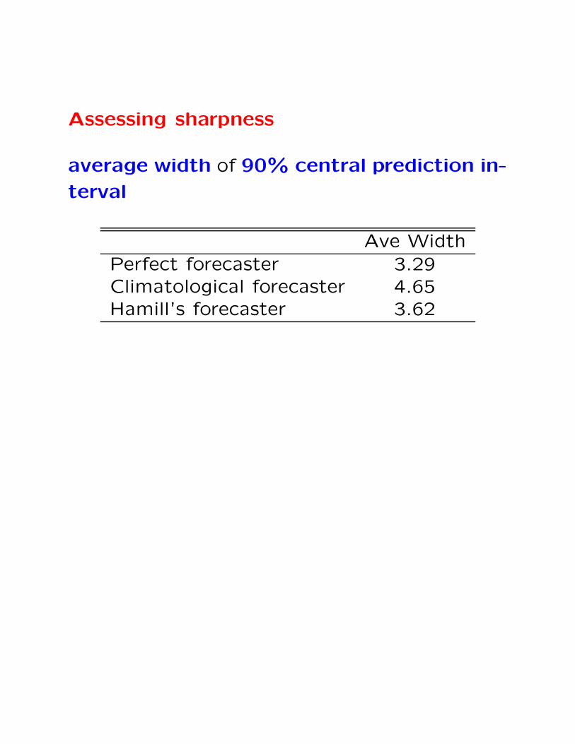
Assessing sharpness
average width of 90% central prediction in-
terval
Ave Width
Perfect forecaster 3.29Climatological forecaster 4.65Hamill’s forecaster 3.62

Scoring rules
a scoring rule
S(F, x)
assigns a numerical score to the forecast/ob-
servation pair (F, x)
negatively oriented: we consider scores to be
penalties
the smaller the better: the forecaster aims
to minimize the average score,
1
T
T∑
t=1
S(Ft, xt)
diagnostic approach: scoring rules address
both calibration and sharpness, yet form one
facet of forecast verification only

Propriety
suppose that I provide probabilistic forecasts
of a real-valued quantity X for your company
my best assessment: G
my actual forecast: F
verification: x
my penalty: S(F, x)
you expect me to quote F = G; however, will
I do so?
only if the expected score is minimized if I
quote F = G, that is if
EG S(G, X) ≤ EG S(F, X)
for all F and G
a scoring rule with this property is called proper
all scoring rules discussed hereinafter are proper

Scoring rules for PDF forecasts
ignorance score (Good 1952; Roulston and
Smith 2002)
IgnS(f, x) = − log f(x)
specifically,
IgnS(N (µ, σ2), x) =1
2ln(2πσ2) +
(x − µ)2
2σ2
quadratic score and spherical score (Good
1971)
QS(f, x) = − f(x) +1
2
∫ ∞
−∞(f(y))2 dy
SphS(f, x) = − f(x)
/(∫ ∞
−∞(f(y))2 dy
)1/2

Scoring rules for predictice CDFs
the continuous ranked probability score or
CRPS has lately attracted attention
origins unclear (Matheson and Winkler 1976;
Stael von Holstein 1977; Unger 1985)
CRPS(F, x) =
∫ ∞
−∞(F (y) − 1(y ≥ x))2 dy
integral of the Brier scores for probability fore-
casts at all possible threshold values y
specifically,
CRPS(N (µ, σ2), x
)
= σ
(x − µ
σerf
(x − µ√
2σ2
)+ 2ϕ
(x − µ
σ
)− 1√
π
)
grows linearly in |x − µ|, in contrast to the ig-
norance score

using results of Szekely (2003)
CRPS(F, x) =
∫ ∞
−∞(F (y) − 1(y > x))2 dy
= EF |X − x| − 1
2EF
∣∣∣X − X ′∣∣∣
where X and X ′ are independent random vari-
ables, both with distribution F
generalizes the absolute error to which it
reduces if F is a deterministic (point) forecast
can be reported in the same unit as the ver-
ifications
provides a direct way of comparing deter-
ministic and probabilistic forecasts
forms a special case of a novel and very general
type of score, the energy score (Gneiting and
Raftery 2004)

Scores for quantile and interval forecasts
consider interval forecasts in the form of the
central (1 − α) × 100% prediction intervals
equivalent to quantile forecasts at the levelsα2 × 100% and (1 −
α2 ) × 100%
α = 0.10 corresponds to the 90% central pre-
diction interval and quantile forecasts at the
5% and 95% level
scoring rule Sα(l, u; x) if the interval forecast
is [l, u] and the verification is x
interval score
Sα(l, u;x) =
2α(u − l) + 4(l − x) if x < l
2α(u − l) if x ∈ [l, u]
2α(u − l) + 4(x − u) if x > u
fixed penalty proportional to width of interval
additional penalty if the verification falls out-
side the prediction interval

Case study:Short-range forecasts of wind speed
wind power: the world’s fastest growing en-
ergy source; clean and renewable
Stateline wind energy center: $300 million
wind project on the Vansycle ridge at the
Oregon-Washington border
2-hour forecasts of hourly average wind speed
at the Vansycle ridge
joint project with 3TIER Environmental Fore-
cast Group, Inc.
data collected by Oregon State University for
the Bonneville Power Administration


Forecast techniques
persistence forecast as reference standard:
Vt+2 = Vt
classical approach (Brown, Katz and Murphy
1984): autoregressive (AR) time series tech-
niques
our approach (Gneiting, Larson, Westrick, Gen-
ton and Aldrich 2004) is spatio-temporal:
regime-switching space-time (RST) method


Regime-switching space-time (RST)
technique
merges meteorological and statistical expertize
model formulation is parsimonious, yet takes
account of all the salient features of wind
speeds: alternating atmospheric regimes, tem-
poral and spatial autocorrelation, diurnal and
seasonal non-stationarity, conditional hetero-
scedasticity and non-Gaussianity
regime-switching: identification of distinct
forecast regimes
spatio-temporal: utilizes geographically dis-
persed meteorological observations in the vicin-
ity of the wind farm
fully probabilistic: provides probabilistic fore-
casts in the form of predictive CDFs

Daily Index
Win
d S
peed
0 1 2 3 4 5 6 7
05
1015
20
21−27 June 2003
| | | | | | | | | | | | | | | | | | | | | | | | | | | | | | | | | | | | | | | | | | | | | | | | | | | | | | | | | | | | | | | | | | | | | | | | | | | | | | | | | | | | | | | | | | | | | | | | | | | | | | | | | | | | | | | | | | | | | | | | | | | | | | | | | | | | | | | | | | | | | | | | | | | | | | | | | | | | | | | |
Daily Index
Win
d S
peed
0 1 2 3 4 5 6 7
05
1015
20
28 June − 4 July 2003
| | | | | | | | | | | | | | | | | | | | | | | | | | | | | | | | | | | | | | | | | | | | | | | | | | | | | | | | | | | | | | | | | | | | | | | | | | | | | | | | | | | | | | | | | | | | | | | | | | | | | | | | | | | | | | | | | | | | | | | | | | | | | | | | | | | | | | | | |
Daily Index
Win
d S
peed
0 1 2 3 4 5 6 7
05
1015
20
5 July − 11 July 2003
| | | | | | | | | | | | | | | | | | | | | | | | | | | | | | | | | | | | | | | | | | | | | | | | | | | | | | | | | | | | | | | | | | | | | | | | | | | | | | | | | | | | | | | | | | | | | | | | | | | | | | | | | | | | | | | | | | | | | | | | | | | | | | | | | | | | | | | | | | | | | | | | | | | |

Verification
evaluation period: May–November 2003
deterministic forecasts: RMSE, MAE
predictive CDFs: PIT histogram, marginal
calibration table, CRPS
interval forecasts (90% central prediction
interval): coverage, average width, interval
score (IntS)
reporting scores month by month allows for
significance tests
for instance, the RST forecasts had a lower
RMSE than the AR forecasts in May, June,
. . . , November
under the null hypothesis of equal skill this will
happen with probability p =(12
)7= 1
128 only

RMSE (m· s−1) May Jun Jul Aug Sep Oct Nov
Persistence 2.14 1.97 2.37 2.27 2.17 2.38 2.11AR 2.01 1.85 2.00 2.03 2.03 2.30 2.08RST 1.75 1.56 1.70 1.78 1.77 2.07 1.88
MAE (m· s−1) May Jun Jul Aug Sep Oct Nov
Persistence 1.60 1.45 1.74 1.68 1.59 1.68 1.51AR 1.54 1.38 1.50 1.54 1.53 1.67 1.53RST 1.32 1.18 1.33 1.31 1.36 1.48 1.37
CRPS (m· s−1) May Jun Jul Aug Sep Oct Nov
AR 1.11 1.01 1.10 1.11 1.10 1.22 1.10RST 0.96 0.85 0.95 0.95 0.97 1.08 1.00
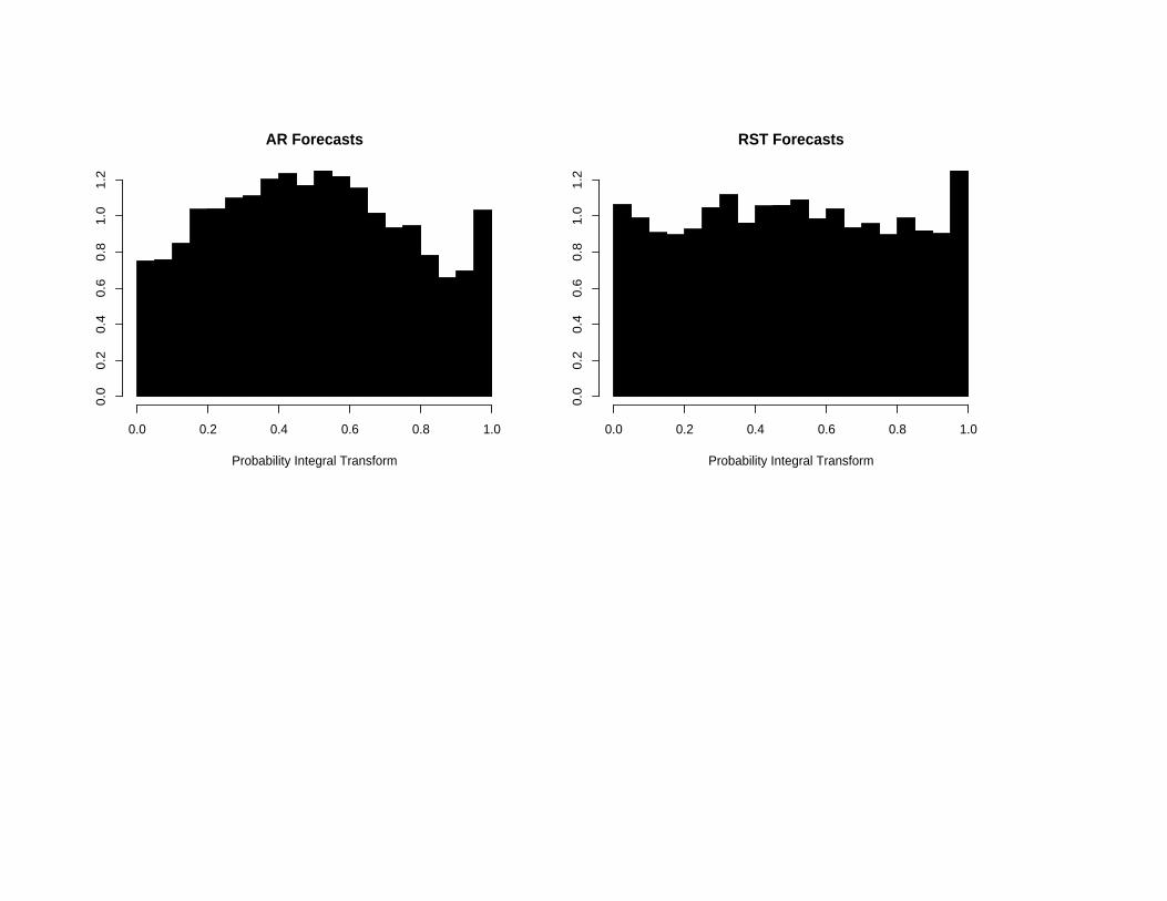
Probability Integral Transform
0.0 0.2 0.4 0.6 0.8 1.0
0.0
0.2
0.4
0.6
0.8
1.0
1.2
AR Forecasts
Probability Integral Transform
0.0 0.2 0.4 0.6 0.8 1.0
0.0
0.2
0.4
0.6
0.8
1.0
1.2
RST Forecasts
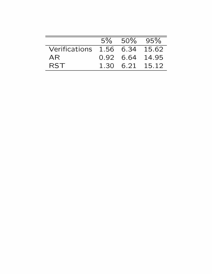
5% 50% 95%
Verifications 1.56 6.34 15.62AR 0.92 6.64 14.95RST 1.30 6.21 15.12

Cov May Jun Jul Aug Sep Oct Nov
AR 91.1% 91.7% 89.2% 91.5% 90.6% 87.4% 91.4%RST 92.1% 89.2% 86.7% 88.3% 87.4% 86.0% 89.0%
Width May Jun Jul Aug Sep Oct Nov
AR 6.98 6.22 6.21 6.38 6.37 6.40 6.78RST 5.93 4.83 5.14 5.22 5.15 5.45 5.46
IntS May Jun Jul Aug Sep Oct Nov
AR 1.74 1.64 1.77 1.75 1.74 2.04 1.86RST 1.52 1.29 1.41 1.50 1.50 1.83 1.64
Technical reports
www.stat.washington.edu/tilmann
Gneiting, T. and A. E. Raftery (2004)
Strictly proper scoring rules, prediction,
and estimation∗
Technical Report no. 463, Department of
Statistics, University of Washington
Gneiting, T., K. Larson, K. Westrick, M. G.
Genton and E. Aldrich (2004)
Calibrated probabilistic forecasting at the
Stateline wind energy center: The regime-
switching space-time (RST) method
Technical Report no. 464, Department of
Statistics, University of Washington
∗Introduces scores as positively oriented rewards ratherthan negatively oriented penalties