Assessing climate change impacts on extreme weatherevents: the case for an alternative (Bayesian) approach

Michael E. Mann1 & Elisabeth A. Lloyd2 & Naomi Oreskes3

Received: 5 June 2016 /Accepted: 19 January 2017 /Published online: 28 August 2017# Springer Science+Business Media B.V. 2017

Abstract The conventional approach to detecting and attributing climate change impacts onextreme weather events is generally based on frequentist statistical inference wherein a nullhypothesis of no influence is assumed, and the alternative hypothesis of an influence is acceptedonly when the null hypothesis can be rejected at a sufficiently high (e.g., 95% or Bp = 0.05^) levelof confidence. Using a simple conceptual model for the occurrence of extreme weather events, weshow that if the objective is tominimize forecast error, an alternative approachwherein likelihoodsof impact are continually updated as data become available is preferable. Using a simple Bproof-of-concept,^ we show that such an approach will, under rather general assumptions, yield moreaccurate forecasts. We also argue that such an approach will better serve society, in providing amore effective means to alert decision-makers to potential and unfolding harms and avoidopportunity costs. In short, a Bayesian approach is preferable, both empirically and ethically.

1 Introduction

There is a growing body of research dealing with the issue of detecting and attributing theimpact of anthropogenic climate change on various types of weather and climate phenomena(e.g., Stott et al. 2013; Bindoff et al. 2013). In recent years, attention has turned in particular tothe impact climate change may be having on extreme weather phenomena (Trenberth 2011;

Climatic Change (2017) 144:131–142DOI 10.1007/s10584-017-2048-3

A comment to this article is available at doi:10.1007/s10584-017-2049-2

Electronic supplementary material The online version of this article (doi:10.1007/s10584-017-2048-3)contains supplementary material, which is available to authorized users.

* Michael E. Mannmann@psu.edu

1 Department of Meteorology and Atmospheric Science, Penn State University, University Park, PA16802, USA

2 History and Philosophy of Science Department, Indiana University, 652 Ballantine Hall,Bloomington, IN 47405, USA

3 History of Science Department, Harvard University, Cambridge, MA 02138, USA

Allen 2011; Blanchet and Davison 2011; Peterson et al. 2012; Otto et al. 2012; Cooley et al.2007; NRC 2016). The traditional approach in these studies involves the use of parallel modelsimulations that alternately have and have not been subjected to anthropogenic increases ingreenhouse gas concentrations. If a particular phenomenon of interest (e.g., record heat, heatwave duration, droughts, floods, or active tornado or hurricane seasons) is found to occursufficiently more often in the latter case than in the former, it is concluded that a change hasbeen detected and can be attributed to the impact of climate change. Among other assumptions,this approach assumes that the models capture the full range of processes that may impact theoccurrence of extreme weather events. That assumption has been disputed by some leadingscientists (Francis and Vavrus 2012; Trenberth 2011, 2012; Trenberth et al. 2015) and has longbeen recognized as a problem in all modeling (Oreskes et al. 1994).

Some researchers have proposed a Bayesian framework for climate change detection andattribution (Berliner et al. 2000), while other researchers have used approaches (see Hegerl et al.2010) that sidestep the detection step or, e.g., employ fractional attributed risk (BFAR^; see, e.g.,Bellprat and Doblas-Reyes 2016) which can avoid the assumptions of frequentist statistics inclimate change attribution. Nonetheless, numerous recent studies (IPCC 2013; Allen 2011;Herring et al. 2015) have continued to invoke a frequentist detection and attribution approachwherein a null hypothesis of no impact is invoked, and rejection of the null hypothesis andalleged detection and attribution of a climate change impact demands rejection of the nullhypothesis at a high level of likelihood (e.g., p = 0.05 or p = 0.10). To quote the most recentIPCC chapter on Detection and Attribution (emphasis added by us), BAttribution results aretypically expressed in terms of conventional ‘frequentist’ confidence intervals or results ofhypothesis tests: when it is reported that the response to anthropogenic GHG increase is verylikely greater than half the total observed warming, it means that the null hypothesis that theGHG-induced warming is less than half the total can be rejected with the data available at the10% significance level. Expert judgment is required in frequentist attribution assessments, but itsrole is limited to the assessment of whether internal variability and potential confounding factorshave been adequately accounted for, and to downgrade nominal significance levels to accountfor remaining uncertainties. Uncertainties may, in some cases, be further reduced if priorexpectations regarding attribution results themselves are incorporated, using a Bayesian ap-proach, but this is not currently the usual practice.^

This philosophical approach to hypothesis testing—i.e., the frequentist framework—iswidespread in the scientific community and it is common to many physical and socialscientific disciplines. Indeed, it is so pervasive that some practitioners conflate it with Bthescientific method,^ and consider it inappropriate even to question whether it provides anappropriate interpretational framework for all scientific hypotheses (see Curry 2011; Allen2011). Yet, despite the sense that it is deeply engrained in the history of science, its roots arerather shallow, with widespread adoption of the practice dating back only to the 1940s(Gigerenzer et al. 1989). Scientists in several fields are increasingly re-examining the appro-priateness of the frequentist approach to hypothesis testing (Nuzzo 2014).

Some have argued that this philosophical framework is a by-product of the intrinsic conser-vatism of the scientific discipline, reflecting a tendency among scientists for Bleast drama^ indrawing inferences and conclusions (Brysse et al. 2013; Anderegg et al. 2014). In practice, thisapproach embraces (see Lloyd and Oreskes, in review) a subjective preference for risking type 2errors of statistical inference (failure to reject a false null hypothesis, i.e., Bfalse negative^) overtype 1 errors (rejecting a true null hypothesis, i.e., Bfalse positive^). In the context of climatescience, it is likely that attacks on scientists by critics, and the ensuing phenomenon of Bseepage,^

132 Climatic Change (2017) 144:131–142

whereby scientists are induced to be cautious for fear of being a target of politically-motivatedcriticism (Lewandowsky et al. 2015), reinforces this latent tendency.

However, in many areas of biomedicine and in pharmaceutical testing, where the principle ofBfirst, do no harm^ prevails, the standard practice (and in some cases legal requirement) is toassume harm until safety can be demonstrated (Gigerenzer and Edwards 2003). With human-caused climate change, there is a potential for greatly increased damage and loss of life, andinaction comes at a large potential societal cost. In this regard, one may argue that climate changeattribution is more like biomedicine than it is, for example, like experimental psychology. Becauseof the potential for harm, the overly conservative frequentist framework is ethically concerning.

An alternative Bayesian framework (Berliner et al. 2000) has been proposed wherein oneemploys as a statistical prior, the evidence that exists—either theoretical or observational innature—that climate change may be impacting the underlying statistical distribution of theclimate variable/s of interest. (Indeed, the alternative Bayesian framework was advocateddecades ago in the field of clinical pharmacology, e.g., Berry 1987). In the case of impactson extreme weather, some researchers (Trenberth 2011, 2012, Trenberth et al. 2015; Lloyd andOreskes (in review)) have proposed that one employs a conditional approach, by accepting apriori relevant physical principles regarding the relationship between climate and extremeweather. For example, the demonstrated warming of the planet has increased the likelihood ofdaily heat extremes (Meehl et al. 2007). Moreover, it has fundamentally intensified the globalhydrological cycle, increasing overall levels of atmospheric humidity and the potential forextreme precipitation events (Trenberth et al. 2015). These considerations provide theoreticaland mechanistic reasons—one might say priors—to believe that climate change is likely to beimpacting extreme weather events. In sum, the Bayesian framework has the advantage, indetection and attribution practices, of having its conclusions be more clearly traceable to theunderlying assumptions and dependence of results on prior assumptions.

The impacts of climate change may be compound in nature for certain types of extremeweather events. For example, with extreme precipitation events, there is both a thermodynamiccomponent (warmer temperatures favor greater atmospheric humidity) and a dynamicalcomponent (upward vertical motion is required for condensation of moisture). In the case oftornadoes, there are likewise thermodynamic (warmer temperatures favor increased moistenergy in the atmosphere) and dynamical factors (greater atmospheric wind shear favors thetwisting of the atmosphere required for tornadic circulation) involved.

The projected changes in the underlying thermodynamic factors are typically better knownthan those in the dynamical factors, and some researchers have argued that we can draw inferencesabout extreme heat and extreme rainfall events based on the thermodynamic considerations (e.g.,Shepherd 2014; Trenberth 2011, 2012; Trenberth et al. 2015). Others (e.g., Stott et al. 2016) haveargued that as long as projected dynamical factors remain uncertain, it is not possible to drawreliable inferences about the impact that climate change will have on these events.

However, the latter argument implicates its advocates in a fallacy: that because we do not knowall underlying factors with certainty, we are unable to say anything about the impact of climatechange on a particular type of weather event. Consider, for simplicity, the case where the impactsof the two factors (thermodynamic and dynamical) are multiplicative and independent. In such acase, if we know with some considerable confidence (e.g., 90% likelihood) that the thermody-namic factors will favor an increase in the frequency of the extreme weather events in question,while dynamical factors are considered a toss-up (i.e., 50% likelihood), then the joint probability(70% likelihood of an increase) is far from a toss-up. Such considerations are explored in moredetail by Shepherd (2016) and are implicit in the recent work of Diffenbaugh et al. (2015).

Climatic Change (2017) 144:131–142 133

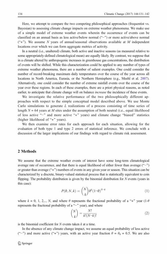
Here, we attempt to compare the two competing philosophical approaches (frequentist vs.Bayesian) to assessing climate change impacts on extreme weather phenomena. We make useof a simple model of extreme weather events wherein the occurrence of events can beclassified on an annual basis as less active/below normal (B−^) or more active/above normal(B+^). We assume N years of annual/seasonal observations available at M independentlocations over which we can form aggregate metrics of activity.

In a neutral (i.e., unaltered) climate, both active and inactive seasons (as measured relative tosome appropriately-defined climatological mean) are equally likely. By contrast, we suppose thatin a climate altered by anthropogenic increases in greenhouse gas concentrations, the distributionof events will be shifted. While this characterization could be applied to any number of types ofextreme weather phenomena, there are a number of salient examples. One could consider thenumber of record-breaking maximum daily temperatures over the course of the year across alllocations in North America, Eurasia, or the Northern Hemisphere (e.g., Meehl et al. 2007).Alternatively, one could consider the number of extreme rainfall events over the course of theyear over these regions. In each of these examples, there are a priori physical reasons, as notedearlier, to anticipate that climate change will on balance increase the incidence of these events.

We investigate the relative performance of the two philosophically different ap-proaches with respect to the simple conceptual model described above. We use MonteCarlo simulations to generate L realizations of a process consisting of time series oflength N = 64 years at M sites under the assumption of both neutral (i.e., equal likelihoodof less active B−^ and more active B+^ years) and climate change Bbiased^ statistics(higher likelihood of B+^ years).

We then examine error rates for each approach for each situation, allowing for theevaluation of both type 1 and type 2 errors of statistical inference. We conclude with adiscussion of the larger implications of our findings with regard to climate risk assessment.

2 Methods

We assume that the extreme weather events of interest have some long-term climatologicalaverage rate of occurrence, and that there is equal likelihood of either fewer than average (B−^)or greater than average (B+^) numbers of events in any given year or season. This situation can becharacterized by a discrete, binary-valued statistical process that is statistically equivalent to coinflipping. The probability distribution is given by the binomial distribution for N events (years inthis case):

P θ;N ; kð Þ ¼ N

k

� �θk 1−θð ÞN−k ð1Þ

where k = 0, 1, 2,.., N, and where θ represents the fractional probability of a B+^ year (1-θrepresents the fractional probability of a B−^ year), and where

N

k

� �¼ N !

k! N−kð Þ! ð2Þ

is the binomial coefficient for N events taken k at a time.In the absence of any climate change impact, we assume an equal probability of less active

(B−^) and more active (B+^) years, with an active year fraction θ = θ0 = 0.5. We are also

134 Climatic Change (2017) 144:131–142

interested in the alternative hypothesis that climate change has led to an increase in theoccurrence of events. That situation is characterized by a probability θ =θ0 > 0.5 for active(B+^) years. Note that for cases (like heat extremes, heat waves, flood frequency) whereclimate change can be a priori assumed to lead to an increase in likelihood, we are dealing one-sided statistical inferences and a one-tailed analysis of any change in the underlying probabilitydistribution

In the conventional, frequentist approach to detection and attribution, we adopt a nullhypothesis H0 of an equal probability of active and inactive years (θ =θ0 = 0.5). We reject it infavor of the alternative hypothesis H1 of a bias toward more active years (θ = θ0 > 0.5) onlywhen we are able to achieve rejection of H0 at a high (we choose the conventional criticalvalue p = 0.05) level of confidence. Once we determine that the null hypothesis can be rejectedat the p = 0.05 level, we replace the prior assumed value θ = 0.5 with the value of θ determinedfrom the accumulated raw data for the site. We do this for each of the M = 100 sitesindependently and only in the end aggregate the statistical results to define a domain-widemetric of occurrence frequency.

In the alternative, Bayesian approach, we assume (1) to represent a likelihood function for θconditional on the available observations. As a prior, we assume an unbiased process (θ = 0.5),admitting both informative (e.g., pre-specified binomial distribution centered at θ = θ0 = 0.5) oruninformative (e.g., uniform over [0, 1]) prior distributions. As increasingly large numbers ofdata N become available, we obtain a posterior distribution of the form of (1) via BayesTheorem:

P AjBð Þ ¼ P BjAð ÞP Að ÞP Bð Þ ð3Þ

where P(A) is the prior, P(B|A)/P(B) is the likelihood function given the data B, and P(A|B) isthe resulting posterior distribution, and where the revised estimate θ is defined by the peak ofposterior distribution. Once again, we do the updating for each of the M sites independently,and aggregate results in the end.

For the purpose of the analysis procedure, we generated via Monte Carlo simulationsof a binary-valued process of length Nmax = 64 for both (a) the unbiased case θ0 = 0.5,(b) the modestly biased case θ0 = 0.6, and (c) the strongly biased case θ0 = 0.75. Thelatter two cases correspond to a 20% higher and 50% higher likelihood, respectively, ofactive (B+^) years vs. inactive (B−^) years. Given, for example, that the rate of record-breaking warmth has doubled (i.e., exhibited a 100% increase) over the past half century(Meehl et al. 2007), our use of a 20 and even 50% increase is, at least for some extremeweather phenomena, conservative.

For each experiment, we performed parallel frequentist and Bayesian estimation of expect-ed values for increasingly large subsets of the data series of length Ntot, iteratively refining ourestimates of the posterior distribution and bias (b = θ0 − 0.5). We performed six sub-experiments that consist of using the first Ntot = 2, 4, 8, 16, 32, and 64 years of the total ofNmax = 64 years of data for each site. These six experiments introduce, sequentially N = 2, 2, 4,8, 16, and 32 new years of data, respectively. For each set, we computed the expected (Ñ+)number of active years based on updated estimates of θ0 derived from the posterior distributionof the previous experiment.

For both methods, we defined an error function ε as the average over all M sites of theabsolute difference between the observed (N+) and predicted (Ñ+) number of active years,allowing us to objectively compare the performance of the frequentist and Bayesian

Climatic Change (2017) 144:131–142 135

approaches. The absolute error is a reasonable proxy for quantities, such as total accrueddamage, that might be of interest in the context of climate change risk.

For a single binary process with nearly equal probabilities (i.e., θ0 = 0.5 to 0.6) for the two(less active and more active) states, the signal-to-noise ratios for the bias b = θ0 − 0.5 arerelatively low. However, aggregating over a set of independent sites M leads to a considerablybetter estimate of the signal.

We show results based on both (a) a large (M = 100) spatial array of sites that can bethought of, conceptually, as an average over a continental (e.g., US-wide) domain, and (b) asmaller (M = 5) spatial array that can be thought of conceptually as representing an averageover a local region (e.g., central Pennsylvania). In both cases, we average the spatial-meanstatistics over a large (L = 100) number of independent realizations to get representativeestimates. For the Bayesian analysis, we have employed a modestly informative prior corre-sponding to the binomial distribution P(θ = 0.5, k = 2, N = 4). Similar results are obtained forthe uninformative uniform prior [0 1].

Our approach represents a simplification of the real world impact of climate change onextremeweather, and this is indeed the point. The simplicity of the proof-of-concept we providespeaks to the generality of the underlying approach and the broad likely applicability of theconclusions drawn. We suggest that there are a number of potential extensions of the approachthat are worth pursuing. Among them is the use of a steadily changing climate (rather than thesimple binary biased/unbiased before/after approach taken), including allowing for scenariossuch as accelerating climate change impacts and/or tipping point-like transitions.

3 Results and discussion

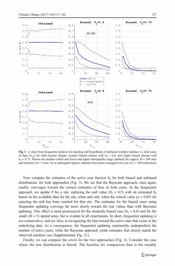
In the frequentist analysis, the distribution of p values for rejecting the null remains centered atp = 0.5 in the case of the unbiased distribution, as it should (Fig. 1). The small number of falsepositives (~ 2 per site breach the p = 0.05 level on average for the M = 100 site experiments)are consistent with chance expectations. In the case of the biased distribution, by contrast, thereis instead a clear trend toward rejecting the null as Ntor increases. As we approach Ntor = 64, wefind that the median of the distribution just breaches the p = 0.05 threshold for the modestlybiased case (θ0 = 0.6), indicating that the null hypothesis of an unbiased distribution is nowbeing rejected at roughly half the sites. For the strongly biased case (θ0 = 0.75), we observemuch more rapid convergence toward rejection of the null, with more than 50% of the sitesbreaching the p = 0.05 threshold at Ntor = 16 and more than 75% of the sites at Ntor = 32. Thesmaller array of sites (M = 5) yields slightly slower convergence toward the rejection of thenull, e.g., the median still lies above the p = 0.05 threshold for the modestly biased case atNtor = 64. The frequentist approach, in short, yields the expected results.

In the Bayesian analysis (Fig. 2), by contrast, we find that posterior distributions efficientlyconverge toward the correct values for both the unbiased (θ0 = 0.5) and biased (θ0 = 0.6 andθ0 = 0.75) cases, as the number of years increases to Ntor = 32 and then Ntor = 64 years. Thedistributions both approach the correct mean value and narrow in width and uncertainty asmore data become available. For the modestly biased case θ0 = 0.6 and M = 100 sites, only asmall fraction (~ 5%) of the total area under the distribution lies to the left of θ0 = 0.5 forNtor = 64, consistent with the observation above (Fig. 1) that the median p value breaches thep = 0.05 significance level for Ntor = 64.

136 Climatic Change (2017) 144:131–142

Now compare the estimates of the active year fraction θ0 for both biased and unbiaseddistributions, for both approaches (Fig. 3). We see that the Bayesian approach, once again,readily converges toward the correct estimates of bias in both cases. In the frequentistapproach, we update θ for a site, replacing the null value (θ0 = 0.5) with an estimated θ0based on the available data for the site, when and only when the critical value (p = 0.05) forrejecting the null has been reached for that site. The estimates for the biased cases usingfrequentist updating converge far more slowly toward the true values than with Bayesianupdating. This effect is most pronounced for the modestly biased case (θ0 = 0.6) and for thesmall (M = 5) spatial array, but is evident in all experiments. In short, frequentist updating istoo conservative, and too slow, to recognizing the bias toward the active state that exists in theunderlying data. As a consequence, the frequentist updating consistently underpredicts thenumber of active years, while the Bayesian approach yields estimates that closely match theobserved numbers (see Supplementary Fig. S1).

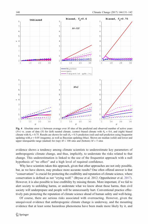
Finally, we can compare the errors for the two approaches (Fig. 4). Consider the casewhere the true distribution is biased. The baseline for comparison then is the steadily

Fig. 1 p value from frequentist analysis for rejecting null hypothesis of unbiased weather statistics vs. total yearsof data (Ntot) for (left) neutral climate, (center) biased climate with θ0 = 0.6, and (right) biased climate withθ0 = 0.75. Shown are median (solid) and lower and upper interquartile range (dashed) for (upper) M = 100 sitesand (bottom)M = 5 sites. As in subsequent figures, statistics have been averaged over a set of L = 100 realizations

Climatic Change (2017) 144:131–142 137

increasing absolute error associated with the null prediction of an unbiased distribution.For the strongly biased case θ0 = 0.75 with large (M = 100) spatial array, whereconvergence toward the true distribution is efficient for either method, the errors forboth frequentist and Bayesian updating level off rapidly to the asymptotic constantbackground value. For the biased case θ0 = 0.6, however, the errors using frequentistupdating continue to grow with sample size through N = 32, while the errors for theBayesian approach remain substantially smaller and nearly level as the posterior distri-bution becomes tighter and more accurate with increasing N. The errors for the Bayesianprediction also remain lower than those for frequentist updating for the small spatial(M = 5) spatial array in both modestly and strongly biased cases.

While the Bayesian updating reduces errors when a bias is present, such reduced errormight be offset by greater error when there is no bias present. Such increased error couldresult from more frequent false positives (i.e., spurious estimates of θ that depart fromthe true value of 0.5). However, we see that this effect is modest, as errors are similar forthe two approaches in the unbiased case. That conclusion holds most strongly for thelarge array (M = 100) of sites (Fig. 4).

Fig. 2 Prior and posterior probability distributions from Bayesian analysis for the active year fraction (θ) for(left) neutral climate, (center) biased climate with θ0 = 0.6, and (right) biased climate with θ0 = 0.75. Shown areprior distribution (red), and posterior distributions for intermediate Ntot = 32 (green) and final Ntot = 64 (black)distributions. Shown are median (solid) and lower and upper interquartile range (dashed) for (top) M = 100 sitesand (bottom) M = 5 sites

138 Climatic Change (2017) 144:131–142

4 Ethical considerations in climate change attribution

We have argued for the Bayesian approach on the intellectual grounds that it offers agreater likelihood of producing empirically accurate results in detection and attributionstudies. This argument is reinforced by the ethical considerations of climate changeattribution. It is well established that the conventional frequentist approach poses agreater risk of type 2 rather than type 1 error. In climate change detection andattribution, this means that we will tend to underestimate the danger represented byextreme events that have been worsened, or made more probable, by an anthropogeniccomponent (Anderegg et al. 2014). This in turn means that society may underpreparefor real threats, increasing the likelihood that property damage, injury, and loss of lifewill ensue (Lloyd and Oreskes, in review).

One might therefore argue that scientists should Berr on the side of caution^ and takesteps to ensure that we are not underestimating climate risk and/or underestimating thehuman component of observed changes. Yet, as several workers have shown (Rahmstorfet al. 2007; Brysse et al., 2013), the opposite is the case in prevailing practice. Available

Fig. 3 Estimated active year fraction (θ0) for (left) neutral climate, (center) biased climate with θ0 = 0.6, and(right) biased climate with θ0 = 0.75 as a function of total years of data (Ntot). Results are shown for frequentistupdating with p = 0.05 (magenta), as well as Bayesian updating (blue). Shown are median (solid) and lower andupper interquartile range (dashed) for (upper) M = 100 sites and (bottom) M = 5 sites

Climatic Change (2017) 144:131–142 139

evidence shows a tendency among climate scientists to underestimate key parameters ofanthropogenic climate change, and thus, implicitly, to understate the risks related to thatchange. This underestimation is linked to the use of the frequentist approach with a nullhypothesis of Bno effect^ and a high level of required confidence.

Why have scientists taken this approach, given that other approaches are not only possible,but, as we have shown, may produce more accurate results? One often offered answer is thatBconservatism^ is crucial for protecting the credibility and reputation of climate science, whereconservatism is defined as not Bcrying wolf.^ (Brysse et al. 2012; Oppenheimer et al. 2017).However, it is also possible to lose credibility by missing threats. More important, if we fail toalert society to unfolding harms, or understate what we know about those harms, then civilsociety will underprepare and people will be unnecessarily hurt. Conventional practice effec-tively puts protecting the reputation of climate science ahead of human safety and well-being.

Of course, there are serious risks associated with overreacting. However, given theunequivocal evidence that anthropogenic climate change is underway, and the mountingevidence that at least some hazardous phenomena have been made more likely by it, and

Fig. 4 Absolute error (ε) between average over M sites of the predicted and observed number of active years(N+) vs. years of data (N) for (left) neutral climate, (center) biased climate with θ0 = 0.6, and (right) biasedclimate with θ0 = 0.75. Results are shown for null (θ0 = 0.5) prediction (red) and null prediction using frequentistupdating with p = 0.05 (magenta), as well as Bayesian updating (blue). Shown are median (solid) and lower andupper interquartile range (dashed) for (top) M = 100 sites and (bottom) M = 5 sites

140 Climatic Change (2017) 144:131–142

given the observed slow response of civil society to act to prevent those harms, it seemsreasonable to conclude that the risks of underreaction to climate change are now greaterthat the risks of overreaction. We suggest that in such a situation, it is ethically preferableto embrace an approach that avoids understating what we know. Fortunately, as we haveshown, this approach is intellectually preferable as well.

5 Conclusions

Using a simple conceptual model for the occurrence of extreme weather events, we showthat the traditional frequentist approach to hypothesis testing, under a fairly general set ofassumptions, suffers from a tendency to underestimate potential climate change impacts onthe occurrence of extreme weather events when such an impact is present in the data. Thatunderestimation, and the error associated with it, tends to increase substantially over time.An alternative Bayesian updating approach does not suffer from this problem.

The dominant current paradigm used in the field of detection and attribution is to employ afrequentist approach, requiring a very high threshold of significance (e.g., p = 0.05) forrejecting the null hypothesis of no impact. We argue that this paradigm is conceptually flawed,empirically damaging, and ethically questionable. It comes at a significant cost to the empiricalaccuracy of detection, leads to delayed detection and a weakened ability to respond to suchdetection, and increases the overall likelihood of underpreparedness for climate-related harms.

If the objective is to minimize forecast error and potential damage, an alternative Bayesianapproach wherein likelihoods of impact are continually updated as data become available ispreferable. We have shown that such an approach will, under rather general assumptions, yieldmore accurate forecasts. Indeed, a proof-of-concept for how scientists might employ aBayesian approach to detection and attribution has already been outlined in the literature(Berliner et al. 2000). It is our recommendation that such an approach be pursued morevigorously in future work. Such an approach would be better both empirically and ethically.

Acknowledgements We thank James V. Stone, Psychology Department, Sheffield University, Sheffield,England for kindly posting the Bayesian coin flipping routine (MatLab code version 7.5. downloaded fromhttp://jim-stone.staff.shef.ac.uk/BayesBook/Matlab). We thank two anonymous reviewers for the helpfulcomments on the initial draft of this article.

References

Allen M (2011) In defense of the traditional null hypothesis: remarks on the Trenberth and Curry WIREs opinionarticles. WIREs Clim Change 2:931–934. doi:10.1002/wcc.145

Anderegg WR, Callaway ES, Boykoff MT, Yohe G, Root TYL (2014) Awareness of both type 1 and 2 errors inclimate science and assessment. Bull Am Meteorol Soc 95:1445–1451

Bellprat O, Doblas-Reyes F (2016) Attribution of extreme weather and climate events overestimated byunreliable climate simulations. Geophys Res Lett 43:2158–2164

Berliner LM, Levine RA, Shea DJ (2000) Bayesian climate change assessment. J Clim 13:3805–3820Berry DA (1987) Interim analysis in clinical trials: the role of the likelihood principle. Amer Stat 41:117–122Bindoff NL, Stott PA, Achuta Rao KM, Allen MR, Gillett N, Gutzler D, Hansingo K, Hegerl G, Hu Y, Jain S,

Mokhov II, Overland J, Perlwitz J, Sebbari R, Zhang X (2013) Detection and attribution of climate change:

Climatic Change (2017) 144:131–142 141

from global to regional. In: Stocker TF, Qin D, Plattner G-K, Tignor M, Allen SK, Boschung J, Nauels A,Xia Y, Bex V, Midgley PM (eds) Climate change 2013: the physical science basis. Contribution of workinggroup I to the fifth assessment report of the intergovernmental panel on climate change. CambridgeUniversity Press, Cambridge

Blanchet J, Davison AC (2011) Spatial modeling of extreme snow depth. Ann Appl Stat 5:1699–1725Brysse K, Oreskes N, O’Reilly J, Oppenheimer M (2013) Climate change prediction: erring on the side of least

drama? Glob Environ Chang 23(1):327–337Cooley D, Nychka D, Naveau P (2007) Bayesian spatial modeling of extreme precipitation return levels. J Am

Stat Assoc 102(479):824–840, Applications and case studies. doi:10.1198/016214506000000780Curry JA (2011) Nullifying the climate null hypothesis. WIREs Clim Change 2:919–924. doi:10.1002/wcc.141Diffenbaugh NS, Swain DL, Touma D (2015) Anthropogenic warming has increased drought risk in California.

Proc Natl Acad Sci U S A 112(13):3931–3936. doi:10.1073/pnas.1422385112Francis JA, Vavrus SJ (2012) Evidence linking Arctic amplification to extreme weather in mid-latitudes.

Geophys Res Lett 39:L06801. doi:10.1029/2012GL051000Gigerenzer G, Edwards A, (2003) Simple tools for understanding risks: from innumeracy to insight, British

Medical Journal, 327, 741–744Gigerenzer G, Switjink Z, Porter T, Daston L, Beatty J, Kruger L (1989) The empire of chance: how probability

changed science and everyday life. Cambridge University Press, CambridgeHegerl GC, Hoegh-Guldberg O, Casassa G, Hoerling MP, Kovats RS, Parmesan C, Pierce DW, Stott PA (2010)

Good practice guidance paper on detection and attribution related to anthropogenic climate change. In:Stocker TF, Field CB, Qin D, Barros V, Plattner GK, Tignor M, Midgley PM, Ebi KL (eds) Meeting reportof the intergovernmental panel on climate change expert meeting on detection and attribution of anthropo-genic climate change. IPCC Working Group I Technical Support Unit, University of Bern, Bern p 8

Herring SC, Hoerling MP, Kossin JP, Peterson TC, Stott PA (2015) Explaining extreme events of 2014 from aclimate perspective. Bull Am Meteorol Soc 96(12):S1–S172

IPCC (2013) Summary for policymakers. In: Stocker TF, Qin D, Plattner G-K, Tignor M, Allen SK, Boschung J,Nauels A, Xia Y, Bex V, Midgley PM (eds) Climate change 2013: the physical science basis. Contribution ofworking group I to the fifth assessment report of the intergovernmental panel on climate change. CambridgeUniversity Press, Cambridge

Lewandowsky S, Oreskes N, Risbey JS, Newell BR, Smithson M (2015) Seepage: climate change denial and itseffect on the scientific community. Glob Environ Chang 33:1–13. doi:10.1016/j.gloenvcha.2015.02.013

Meehl GA, Arblaster JM, Tebaldi C (2007) Contributions of natural and anthro-pogenic forcing to changes intemperature extremes over the U.S. Geophys Res Lett 34:L19709. doi:10.1029/2007GL030948

National Research Council (2016) Attribution of extreme weather events in the context of climate change.National Academies Press, Washington, DC

Nuzzo R (2014) Scientific method: statistical errors. Nature 506:150–152Oppenheimer M, Oreskes N, Jamieson D, Brysse K, O’Reilly J, Shindell M, (2017) Assessing assessments:

scientific knowledge for public policy, University of Chicago Press. (forthcoming)Oreskes N, Shrader-Frechette K, Belitz K (1994) Verification, validation, and confirmation of numerical models

in the earth sciences. Science 263:641–646Otto FEL, Massey N, van Oldenborgh GJ, Jones RG, Allen MR (2012) Reconciling two approaches to

attribution of the 2010 Russian heat wave. Geophys Res Lett 39:L04702. doi:10.1029/2011GL050422Peterson T, Stott P, Herring S (2012) Explaining extreme events of 2011 form a climate change perspective. Bull

Am Meteorol Soc 93(7):1041–1067Rahmstorf S, Cazenave A, Church JA, Hansen JE, Keeling RF, Parker DE, Somerville RC (2007) Recent climate

observations compared to projections. Science 316(5825):709–709Shepherd TG (2014) Atmospheric circulation as a source of uncertainty in climate change projections. Nat

Geosci 7:703–708Shepherd TG (2016) A common framework for approaches to extreme event attribution. Curr Clim Change Rep

2(1):28–38. doi:10.1007/s40641-016-0033-yStott PA, Allen M, Christidis N, Dole RM, Hoerling M, Huntingford C, Pall P, Perlwitz J, Stone D (2013)

Attribution of weather and climate-related events. In: Asrar GR, Hurrell JW (eds) Climate science for servingsociety. Springer, Haarlem, pp 307–337

Stott P, Christidis N, Otto FEL, Sun Y, Vanderlinden J-P, van Oldenborgh GJ, Vautard R, von Storch H, Walton P,Yiou P, Zwiers FW (2016) Attribution of extreme weather and climate-related events. Wiley Interdiscip RevClim Chang 7(1):23–41. doi:10.1002/wcc.380

Trenberth KE (2011) Attribution of climate variations and trends to human influences and natural variability.WIREs Clim Change 2:925–930

Trenberth KE (2012) Framing the way to relate climate extremes to climate change. Clim Chang 115:283–290Trenberth KE et al (2015) Attribution of climate extreme events. Nat Clim Chang 5:725–730

142 Climatic Change (2017) 144:131–142