ASE FILE COPY

ASE FILECOPY

*v

IFSM-72-13

LEfflOI HJNTO1 1ITY

ALTERNATING METHOD APPLIED TOEDGE AND SURFACE CRACK PROBLEMS

byR. J. Hartranft

andG. C . S i h

Technical Report NASA-TR-72-1

April 1972

NATIONAL AERONAUTICS AND SPACE ADMINISTRATION

LANGLEY RESEARCH CENTER

HAMPTON, VIRGINIA 23365

https://ntrs.nasa.gov/search.jsp?R=19730012185 2018-02-12T11:14:24+00:00Z

Page Intentionally Left Blank

\s

I I

ABSTRACT

The Schwarz-Neumann alternating method is employed to obtain stressintensity solutions to two crack problems of practical importance: (1) asemi-infinite elastic plate containing an edge crack which is subjectedto concentrated normal and tangential forces, and (2) an elastic half-space containing a semicircular surface crack which is subjected touniform opening pressure. The solution to the semicircular surfacecrack is seen to be a significant improvement over existing approximatesolutions. Application of the alternating method to other crack prob-lems of current interest is briefly discussed.

Page intentionally Left Blank

NATIONAL AERONAUTICS AND SPACE ADMINISTRATION

Grant NGR-39-007-066

Technical Report No. 1

ALTERNATING METHOD

APPLIED TO

EDGE AND SURFACE CRACK PROBLEMS

by

R. J. HartranftAssistant Professor of Mechanics

and

G. C. SihProfessor of Mechanics

Department of Mechanical Engineering and MechanicsLehigh University

Bethlehem, Pennsylvania

i-'

. > : • • « : - t &X1 Y-V ;~' Apri l- V972

e* Blank

TABLE 0£ CONTENTS

Page

LIST OF FIGURES iii

NOTATION iv

1. INTRODUCTION 1

2. EDGE CRACK PROBLEM 7

2.1 Infinite Plate with a Central Crack 11

2.2 Edge-Loaded Semi-Infinite Plate 19

2.3 Iterative Formulation of the Problem 202.4 Numerical Results and Green's Function 27

i

3. SURFACE CRACK PROBLEM 32

3.1 Penny-Shaped Crack in an Infinite Body 33

3.2 Surface Loads on Half Space 46

3.2(1) Nonsingular stress 46

3.2(2) Singular stress 49

3.3 Iterative Formulation 50

3.4 Numerical Treatment of Singularities 563.4(1) Half space 56

3.4(2) Penny-shaped crack - nonsingular load 583.4(3) Penny-shaped crack - singular load 61

3.5 Discussion of Numerical Results 64

4. FUTURE APPLICATIONS - SEMI-ELLIPTICAL CRACK 66

APPENDIX 70

.REFERENCES - . 78

FIGURES,.. . -••., .'. -•= ' 81.•-i , - ' • • . I 1

Paqe Intentionally Left Blank

List of Figures

Figure Title

2.1 Edge-cracked plate

2.2 Cracked infinite plate

2.3 Edge-loaded half plane

2.4 Concentrated forces on an edge crack

2.5 Stress intensity factor correction for concen-trated forces on an edge crack

3.1 Penny-shaped crack in infinite body

3.2 Local coordinates (p,<}>) at crack front

3.3 Half space (x>;0) loaded on surface (x=0)

3.4 Auxiliary coordinates for singular solutions

3.5 Function for eq.(3.39) for singular normal stresson half-space

3.6 Half-penny surface crack

3.7 Grid rn surface of half-space

3.8 Stress intensity factor for Figure 3.6

3.9 Successive iterations for stress intensity factor

3.10 Separate contributions to the stress intensityfactor in first iteration

,4.1 S e m i - e l l i p t i c a l surface crack

A-l Linearly loaded edge crack

A-2 Partially loaded edge crack

'A-3 ' Correction factors for partially loaded edge crack

A-4 Penny-shaped crack in an infinite body underu n i a x i a l tension and uniform shear

A-5 Concentrated forces on a penny-shaped crack

A-6 Penny-shaped crack in a cross-section of a beamunder pure bending

i i i


NOTATION

A' ° A ' etc' " n solution in sequence A

B ' B ' etc' - n solution in sequence B

E,v ~ modulus of elasticity, Poisson's ratio

J (x) - Bessel function of first kind of orderm m

j (x) - spherical Bessel function of first kindm of order m

Edqe Crack

a - length of edge crack, half length ofcrack in infinite medium

b - distance from edge to concentratedforce

B(a) - arbitrary function in solution ofSection 2.1

c - b/a

f(b/a) - ki, k2 correction for concentratedforces

FQ(y,z) - nonsingular stress on x=0 for uniformpressure on crack

F (y) - function involved in representation ofmn q(y,o)

ki, k2 - stress intensity factors in Mode I, II

k(n), ki") - contribution of nth iteration to ki, k2t \ i \

P (y)> q^(x) - normal stresses on planes x = 0, y=0 inn i teration

P,Q - concentrated forces on the crack

r- V'..\ ' ' " • • > - • ^ ' ' ' • ' " "" ' ' ; ' " ' '• ' d is tance from crack tip

s(n)U), t(n)(u) - dimensionless forms of q(n)(x), p(n)(y)


u = y/(a+y) - variable to reduce infinite range ofintegration to finite range

u , v - displacement componentsx y

v(x) = 2(i-v2) vy(

x'°)> displacement on y = 0

a(x) - normal stress (-a (x,0)) applied tocrack ^

a , a , T - stress componentsx y xyijj(t) - function introduced to solve for v(x)

and B(a)

Surface Crack

a - radius of penny-shaped crack, used tonon-dimensionalize all lengths

A_n - coefficient of rn cos2(m-l)e in expan-mn sion of p(r,9)

b - size of square in half space solution

C - coefficient of tn in expansion of92m-2(t)

D (£) - arbitrary functions in solution ofm Section 3.1

F(£,n,c) - Love's solution for normal stress onz=0 due to unit tension on a square ofx=0 (half space)

g (t) - functions introduced to solve for

nr

- !0 = "/2' 'l = ]' Jk = 'k-2

- stress intensity factor

k(0) - dimensionl ess stress intensity factor,

lv ;k(n-l)(|)ks(e) + k(n)(e), contribu

tion of n iteration to k(e)


kin)(6) - k(9) produced by 0_ = pntin)(x,y) onn crack z u IM

kq(9) - k(9) produced by singular stress(Section 3.4(3)) on crack

K (r) - Fourier coefficients of p(r,6)

p - dimensionless pressure at center ofcrack

P0 - uniform pressure on crack, used tonon-dimensionalize boundary stresses

p(r,e) - dimensionless variable pressure oncrack

dimensionless, nonsingular part of 0j_ L. A

on x=0 in n iteration

qc,n'(y,z) - nonsingular part of 0 on x = 0 producedJl A

by 0 = tJin'(x,y) on crack

qc(y,z) - nonsingular part of 0 on x=0 producedO A

by singular stress (Section 3.4(3)) oncrack

r,9,z - dimensionless cylindrical coordinates

RI> iî, Ra» ^2 - dimensionless coordinates in plane ofcrack

S(i|j) - function giving singular 0 on crackdue to singular part of a on x=0

A

t^n'(x,y) = - k^n" '(|)ts(x,y) + t^n'(x,y), dimen-

sionless, nonsingular stress on crackin n iteration

/ \*M (x,y) - stress on crack produced by

0.. = qin" '(.y,z) on x = 0

VI

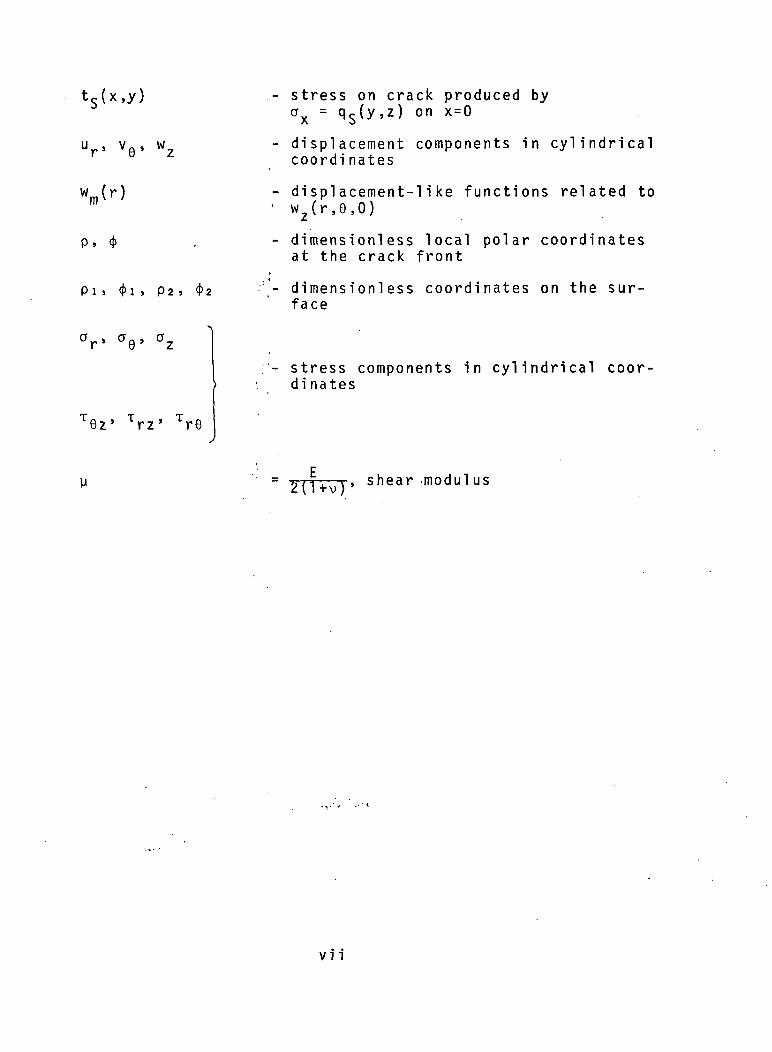
t s ( x , y )

V V wz

w m ( r )

P» 4»

Pis < f > l » P2 , <J>2

- stress on crack produced byax = on

- displacement components in cylindricalcoordinates

- displacement-like functions related to' w2(r,0,0)

- dimensionl ess local polar coordinatesat the crack front

- dimensionl ess coordinates on the sur-face

ar> V az

T6z' Trz' Tr6

stress components in cylindrical coor-dinates

+ \ » shear modulus

VI 1

InteL*ft 8/a

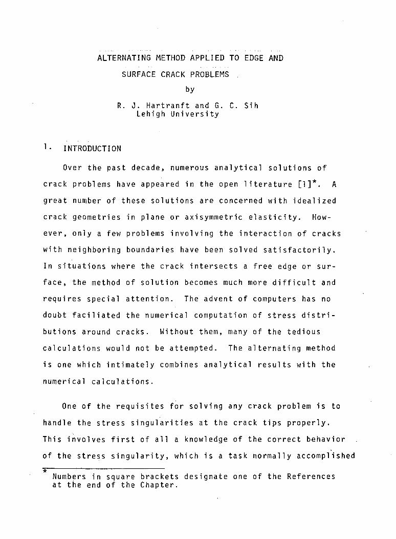
ALTERNATING METHOD APPLIED TO EDGE AND

SURFACE CRACK PROBLEMS

by

R. J. Hartranft and G. C. SihLehigh University

1- INTRODUCTION

Over the past decade, numerous analytical solutions of

crack problems have appeared in the open literature [1]*. A

great number of these solutions are concerned with idealized

crack geometries in plane or axisymmetric elasticity. How-

ever, only a few problems i n v o l v i n g the interaction of cracks

with neighboring boundaries have been solved satisfactorily.

In situations where the crack intersects a free edge or sur-

face, the method of solution becomes much more difficult and

requires special attention. The advent of computers has no

doubt faciliated the numerical computation of stress distri-

butions around cracks. Without them, many of the tedious

calculations would not be attempted. The alternating method

is one which intimately combines analytical results with the

numerical calculations.

One of the requisites for solving any crack problem is to

handle the stress singularities at the crack tips properly.

This involves first of all a knowledge of the correct behavior

of the stress singularity, which is a task normally accomplished

*Numbers in square brackets designate one of the Referencesat the end of the Chapter.

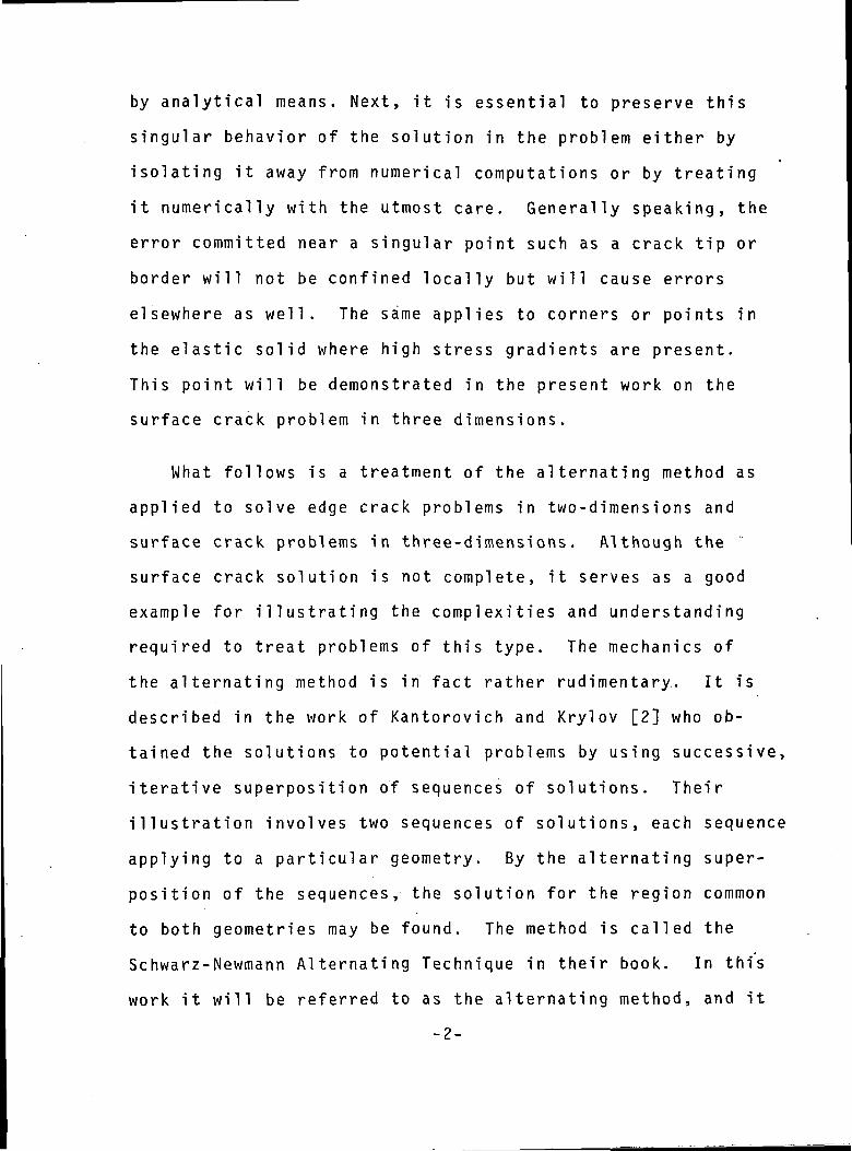
by analytical means. Next, it is essential to preserve this

singular behavior of the solution in the problem either by

isolating it away from numerical computations or by treating

it numerically with the utmost care. Generally speaking, the

error committed near a singular point such as a crack tip or

border will not be confined locally but w i l l cause errors

elsewhere as well. The same applies to corners or points in

the elastic solid where high stress gradients are present.

This point will be demonstrated in the present work on the

surface crack problem in three dimensions.

What follows is a treatment of the alternating method as

applied to solve edge crack problems in two-dimensions and

surface crack problems in three-dimensions. Although the

surface crack solution is not complete, it serves as a good

example for illustrating the complexities and understanding

required to treat problems of this type. The mechanics of

the alternating method is in fact rather rudimentary. It is

described in the work of Kantorovich and Krylov [2] who ob-

tained the solutions to potential problems by using successive,

iterative superposition of sequences of solutions. Their

illustration involves two sequences of solutions, each sequence

applying to a particular geometry. By the alternating super-

position of the sequences, the solution for the region common

to both geometries may be found. The method is called the

Schwarz-Newmann Alternating Technique in their book. In this

work it will be referred to as the alternating method, and it

-2-

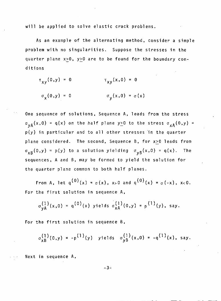
will be applied to solve elastic crack problems.

As an example of the alternating method, consider a simple

problem with no singularities. Suppose the stresses in the

quarter plane x_>0, y>^0 are to be found for the boundary con-

ditions

Txy(0,y) = 0 T

Xy(x'0) = °

ax(0,y) = 0 ay(x,0) = a(x)

One sequence of solutions, Sequence A, leads from the stress

a ,(x,0) = q(x) on the half plane y_>0 to the stress a »(0,y) =

p(y) in particular and to all other stresses 'in the quarter

plane considered. The second, Sequence B, for x^>0 leads from

axB(0,y) = p(y) to a solution yielding a B(x,0) = q(x). The

sequences, A and B, may be formed to yield the solution for

the quarter plane common to both half planes.

From A, let q(0)(x) = a(x), x>0 and q(0)(x) = a(-x), x<0.

For the first solution in sequence A,

ayA}(x,0) = q(0)(x) yields axA

}(0,y) = p(1)(y), say.

For the first solution in sequence B,

axB)(0'y) = -p(1)(y) yields ayB)(x'0) = -q(1)(x),

Next in sequence A,

-3-

j0) = q(1)(x) yields a)(o,y) = p(2)(y), say

and then in sequence B,

,y) = -p(2)(y) yields c^2)(x,0) = -q(2)(x), say

The sequences continue alternating this way. Both sequences

apply to the quarter plane, and by superposition, the boundary

values on the quarter plane are

oy(x,0) =

or

ay(x,0) = q(0)(x) - q(1)(x) + q(1)(x) - q(2)(x)

ax(0,y) -

Therefore, after superposing the first n terms of each sequence,

the boundary values are

ay(x,0) = a(x) - q(n)(x)

ax(0,y) = 0

Additional solutions from the sequences are superposed until

the residual stress, q^(x), on the x-axis is ne g l i g i b l e

-4-

compared to the applied stress a(x).

A different form of the alternating method was applied to

the problem of an edge crack in a semi-infinite region by

Irwin [3], who essentially used only the first few solutions

of each sequence to estimate the stress intensity factor.

Lachenbruch [4] included additional terms from each sequence

to obtain a better estimate. Further study of the alternating

method ap p l i e d to this problem w i l l be carried out in detail

in Section 2. One of the two sequences of solutions involved

there is for an infinite region containing a finite straight-

crack subjected to arbitrary normal stresses on its faces.

The solution is written in integral form and may be evaluated

for any given loads. In this case, the analytical result

gives the singularity separately, and no additional special

numerical treatment is required.

Recently, application of the alternating method to finiteV

width strips cracked on one edge has been formulated by Broz

[5]. The method of Section 2 could be extended to this case

by using three sequences of solutions. Reference to such

extensions will be made later on. However, Broz considers

more complicated analytical problems i n v o l v i n g only two se-

quences. One sequence considers a row of collinear equally

spaced cracks of equal length, each loaded by the same arbi-

trary normal stresses on its faces. He gives the formulas

for the stresses at the locations of the edges of the strip

in terms of integrals which may be numerically evaluated.

-5-

The other sequence gives a similar expression for the stress

produced at the location of the crack in an uncracked strip

loaded arbitrarily on its edges. He has included very few

numerical results in [5], but a computer program for obtaining

additional results could be easily written.

In a similar fashion, three-dimensional problems may also

be solved by the alternating method. Smith et al. [6,7,8]

have published a series of papers containing numerical results

for the effect of interaction of cracks with free surfaces.

One of the geometries considered [6] was a surface crack per-

pendicular to the surface of a half space. The crack is in

the shape of half of a flat circular disk with the diameter

on the surface. The other problems involved cases where the

crack is a larger of smaller portion of the circular disk

whose diameter parallel to the surface lies either above or

below the surface. In [7] the crack intersects the free sur-

face, and in [8] it is completely embedded in the half space.

A generalization of [8] was later made by Shah and Kobayashi

[9] in which the embedded crack is e l l i p t i c a l in shape with

the minor axis perpendicular to the surface.

As in the plane problems, one sequence of solutions for

the three-dimensional problems above is chosen to be an in-

finite body containing a crack. For the penny-shaped crack

a fairly convenient solution is known for pressure on the

crack of the form rncosm6 where r and 0 are the usual polar

coordinates. A less convenient solution for the e l l i p t i c a l

crack is known for polynomial variations of the stress on

-6-

the crack. But these solutions account only partially for

the effect of the stress singularity. The other sequence

used for the three-dimensional problems is made up of solu-

tions of arbitrarily loaded half spaces. It may be seen in

Section 3 that the stress applied to the half space must be

singular. The previous solutions do not satisfactorily

treat this effect, which is shown in Section 3.5 to drasti-

cally alter the numerical results. The singularity on the

surface of the half space may be taken care of analytically,

and then one is faced with an additional singularity in the

other sequence. That is, the stress applied to the crack is

singular at two points of the crack front. No analytical

way of handling this singularity could be found at present,

but special precaution was taken numerically.

2- EDGE CRACK PROBLEM

The determination of stress intensity factors for bodies

containing cracks extending inward from a free edge has at-

tained importance because such cracks are frequently found in

structural members. The analytical model is usually based

on the theory of elasticity in plane strain or generalized

plane stress. The case of a crack perpendicular to the edge

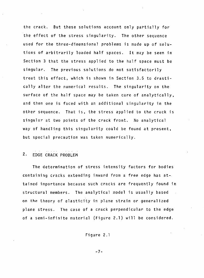
of a semi-infinite material (Figure 2.1) wi l l be considered.

Figure 2.1

-7-

Irwin [3,10] estimated the stress intensity factor, k, ,

for the case of uniform pressure on the edge crack (or uni-

form tension at infinity perpendicular to the crack) and ob-

tained a value of k-, ten percent higher than that for an

infinite plate with a crack of twice the length. He used

two problems whose solutions are given in Sections 2.1 and

2.2. The infinite plate with an arbitrarily pressurized

crack is considered first. Then the half plate subjected to

arbitrary normal stresses is superposed on the infinite

cracked plate. Irwin used the superposition to obtain two

simultaneous integral equations (see Section 2.3) in two

unknown functions and solved them by an iterative method which

is equivalent to the alternating method presented here.

Later, Bueckner [11] reconsidered the problem and ob-

tained a more accurate correction (13%)*. By superposing the

two problems described above, he obtained a singular inte-

gral equation for the deformed shape of the crack. The equa-

tion permitted straightforward integration for obtaining the

pressure required to produce certain prescribed deformed

shapes. A number of different deformed shapes and associated

pressure distributions were obtained. A linear combination of

these pressures was fitted to the actual uniform pressure by

collocation (equating the actual pressure to the linear

Winne and Wundt [12] overlooked the correction of Buecknerwhen they used some of his other results on cracks in finitewidth strips (also contained in [11]). The review of Parisand Sih [1] points out the error in [12].

-8-

combination at a number of points equal to the number of un-

determined coefficients). Thus the deformed shape of th'e

crack was determined as a known linear combination of the

prescribed shapes. And the stress intensity factor followed

immediately (as from equation (2.16) below).

Koiter [13], in his analysis of the same problem, gave a

refined value of the stress intensity factor i n v o l v i n g a cor-

rection of 12.15%. The computation of a definite integral was

done numerically with such precision that the factor above is

in error by no more than one unit in the last digit. The

definite integral results from the application [14] of M e l l i n

transforms [15] to the quarter plane problem to which the one

under consideration reduces by symmetry. The transform leads

to an equation of the WIENER-HOPF type which is then solved.

Table I: k-j values for uniform tension in Figure 2.1

Source

Irwin [3,10]

Bueckner [11]

Koiter [13,14]

W i g g l e s w o r t h [16]

Lachenbruch [4]

S ta l l yb rass [18]

Sneddon [19]

Append ix

Va/a

1

1

1

1

1

1

1

1

.1

.13

.1215

. 122

.1

.1215

.1215

.1215*

obtained by using equation (2.50)

-9-

A more general study of the problem using the alternating

method, was made by Lachenbruch [4], who considered variable

as well as uniform loads on the crack.

There have been other solutions [16,17,18] of the problem

using the same technique as in [13,14]. The latest by

Stallybrass [18] obtains the stress intensity factors for

stress on the crack varying as a power of distance from the

edge. He gives numerical results for integer powers, 0, 1,

2, ••• 10, which could be combined if the stress on the crack

is a polynomial function of that distance. Sneddon [19] also

used the quarter plane formulation, but his technique of

solving the problem (similar to the method of Section 2.1)

leads to a Fredholm integral equation of the second kind. Two

approximate methods of solving the integral equation are com-

pared for the case of uniform stress on the crack, and both

give very good accuracy.

Sections 2.1 and 2.2 which follow contain the solutions

of the two problems used in the alternating method. The

alternating method is presented in detail in Section 2.3 for

the case of concentrated forces acting on the crack. The

numerical results of Section 2.4 are used to develop an inte-

gral expression for the stress intensity factor for arbitrary

loads on the crack. The integral is evaluated for several

examples which are contained in the Appendix. One of the

examples is the problem of uniform pressure on the crack which

has been considered by many others. A comparison of this

-10-

result with those obtained by the various other investigators

can be found in Table I.

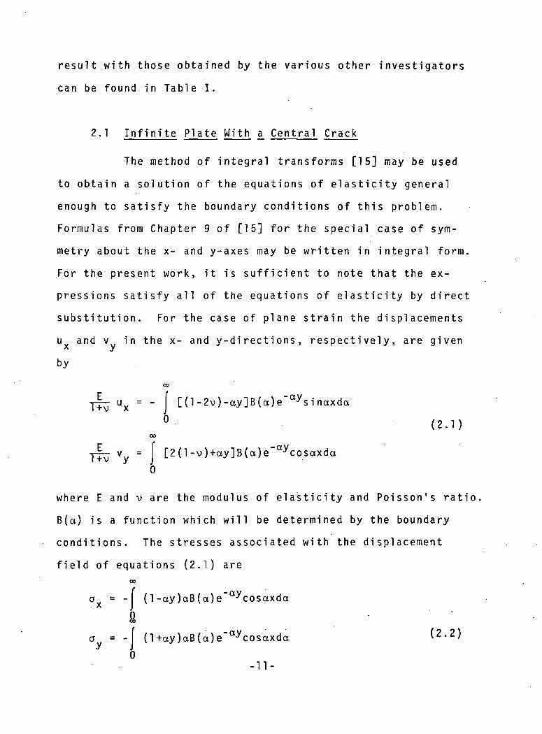
2.1 Infinite Plate With a_ Central Crack

The method of integral transforms [15] may be used

to obtain a solution of the equations of elasticity general

enough to satisfy the boundary conditions of this problem.

Formulas from Chapter 9 of [15] for the special case of sym-

metry about the x- and y-axes may be written in integral form.

For the present work, it is sufficient, to note that the ex-

pressions satisfy all of the equations of elasticity by direct

substitution. For the case of plane strain the displacements

u and v in the x- and y-di rections , respectively, are givenx y

by

ux " • [d-2v)-oy]B(a)e"ays1naxdci0 (2.1)

= I [2(l-v)+ay]B(a)e"aycosaxda

where E and v are the modulus of elasticity and Poisson's ratio

B(a) is a function which w i l l be determined by the boundary

conditions. The stresses associated with the displacement

field of equations (2.1) areoo

a = - (1-ay)aB(a)e"aycosaxda

a = -1 (l+ay)aB(a)e"aycosaxda

0-11-

W

a2B(a)e~a^sinaxdctjxy0

The solution given by equations (2.1) and (2.2) may

also be used for generalized plane stress if E is replaced by

(l+2v)E/(l+v)2 and v by v/(l+v). Equations (2.1) and (2.2)

should be applied only for yÔ. For negative y, the conditions

of symmetry about the x-axis should be used. The crack pro-

blem of this Section is restricted to the case of loading by

normal stresses on the crack which are symmetric about the

y-axis. With this restriction, the problem has the symmetry

required for application of equations (2.1) and (2.2). It

may be noticed that the last of equations (2.2) satisfies the

boundary condition T (x,0) = 0 on the crack and the x-axisxyof symmetry outside of the crack.

Figure 2.2

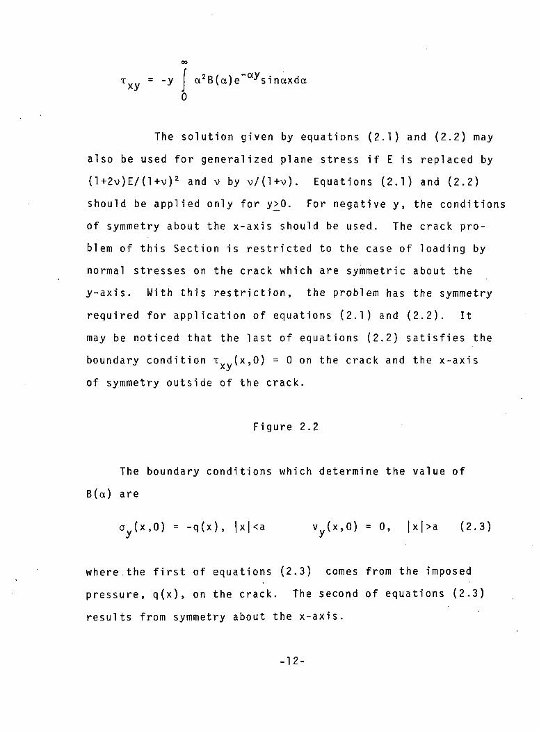
The boundary conditions which determine the value of

B(a) are

a (x,0) = -q(x), |x|<a vy(x,0) = 0, |x|>a (2.3)

where the first of equations (2.3) comes from the imposed

pressure, q(x), on the crack. The second of equations (2.3)

results from symmetry about the x-axis.

-12-

The boundary conditions (2.3) require these special

results from .eqs. (2.1 ) and (2.2):

Y j v y ( x , 0 ) = 2 ( l - v ) B ( a ) c o s a x d a0

7 <2-4)a (x,0) = - aB(a)cosaxda

0CO

Let v(x) = - - - v (x,0) = I B(a)cosaxda (2.5)2(l-v2) y JQ

The Fourier inversion [15] of equation (2.5) gives

oo

B(a) = - v(x)cosaxdx

0

But by the second of equations (2.3), v(x) = 0 for x>a.

Therefore, B(a) becomes

a9 f

B(a) = -jj- v(x)cosaxdx (2.6)

0

Now, since v(x) is a displacement, the representation

a

v' !x

(X) = f t ( t ) t d t f 0<x<a (2i /f 2 _ y 2

may be used. Integration of equation (2.7) by parts shows

the correct crack tip opening shape. If equation (2.7) is

substituted into equation (2.6),

-13-

B ( a ) = —• cosaxdx ^ 'J J /F2T0 x

a t

= £ f <Mt)tdt f ^^77 J J /JTT:cosax dx

0

<Mt)JQ(at)tdt (2.8)*

0

The first of equations (2.3) and the second of (2.4)

give the equation

CO

aB(a)cosaxda = q(x) , 0<x<a (2.9)

0

Integrating equa t i on (2 . 9) ,

00 x

1 B (a )s i naxda = | qU)d£ , 0<x<a (2 .10 )

0 0

If equation (2.8) is substituted into equation(2 . 1 0) an

integral equation for ip(t) results.00 a xf s inaxda f ty(t) J Q (a t ) td t = | q ( C ) d ^ , 0<x<a

0 0 0

a °° xor f i|i(t)tdt [ J Q (a t )s inaxda = | q ( ^ ) d C , 0<x<a (2 .11)

0 0 0

The formula for JQ(X), the Bessel function of order zero',on page 27 of [20] is used in the last step.

-14-

But'

WW

j J0(at)sinaxda = <

0

1

/X2-t2

t>x

t<x

Therefore, equation (2.11) reduces to

q(£)d£ » 0<x<a (2.12)

Equation (2.12) may, be solved as a special cas.e of Abel's

integral equation

x

**

f 4»(t)dt

0 /*rriT= h(x) , 0<x<a (2.13)

which has the solution

= | ft f UKA71 L J /t2-

0<t<a (2.14)

Therefore, the solution of equation (2.12) is

t

*(t) - q(x)dx 0<t<a0

(2.15)

It is known that the opening displacement of the

crack tip is given by (see equations (3.15) of [21])

**First formula on page 37 of [20].

This form may be obtained from that on page 141 of [20] bya change of variables.

-15-

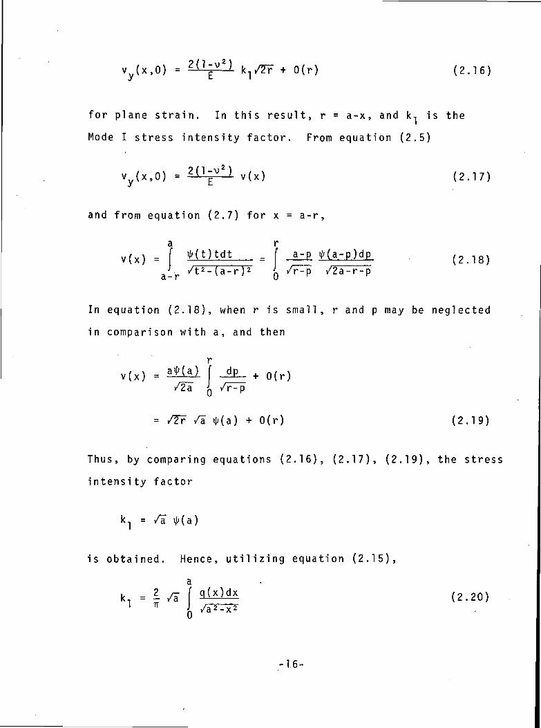
vy(x,0) = 0(r) (2.16)

for plane strain. In this result, r = a-x, and k, is the

Mode I stress intensity factor. From equation (2.5)

vy(x,0) = "v v(x) (2.17)

and from equation (2.7) for x = a-r,

v(x) = f »(t)tdt = " a-p »(a-p)dp>• /t2-(a-r)

2a-r 0 /2a-r-p

(2.18)

In equation (2.18), when r is small, r and p may be neglected

in comparison with a, and then

V(X) =/2~a

0(r)

= /2r /a 0(r) (2.19)

Thus, by comparing equations (2.16), (2.17), (2.19), the stress

intensity factor

= /a

is obtained. Hence, utilizing equation (2.15),

a(2.20)

-16-

It is also necessary to evaluate the normal stress

on the y-axis which, from equations (2.2), is

ax

vw

(0,y) = -j (l-ay)aB(a)e"ayda (2.21)

From equations (2.8) and (2.15)

a t[a) = | | JQ(at)tdt |

0 0

2 f f 0= I q(x)dx -=— - tdt

J0<at>

Therefore, interchanging the order of integration in equation

(2.21),

° (0,y) = f f(x,y)q(x)dx (2.22)^ J

0a

where f(x,y) = f g(y,t) tdt (2.23)J J t 2 _ v 2XCO

where g(y,t) = - (1-ay)aJ0(at)e"ayda

The evaluation of g(y,t) leads directly to

The integration of equation (2.23) may be accomplished with

g(y,t) given by equation (2.24). The result is

-17-

f(x,y) =x2+y2

a2-x2

a2+y2

_2j,2

(2.25)

Finally, substituting equation (2.25) into (2.22), the in-

tegral

1— f q(x)P(y) • f r|_x2+y2 |_x2+y2 a2+y2

(2.26)

for the desired stress,

= p(y) (2.27)

is obtained.

The above results apply also to the case of shear

loading on the crack. In fact if the stress on the crack is

Txy(x,0) = -q(x) , |x|<a

where q(x) = q(-x), then the Mode II stress intensity factor

i sa

q(*)dx (2.28)k, - /a

and

T(0,y) = p(y)

where p(y) is given by equation (2.26)

-18-

2.2 Edge-Loaded Semi-Infinite Plate

The solution given by equations (2.1) and (2.2)

applies to the case in which a half plane, y>^0 (Figure 2.3)

is subjected to normal stresses

oy(x,0) = p(x) (2.29)

symmetric about the y-axis. It is found from the second of

equations (2.2) and the Fourier inversion theorem that

aB

CO

(a) = - | I p(x)cosaxdx . (2.30)

Figure 2.3

The first of equations (2.2) and equation (2.30)

combine to give

ax

\*J <JW

(0,y) = — (1-ay)ae"ayda p ( x ) c o s a x d x

-0 000 00

= — p(x)dx (1-ay)ae~aycosaxda

0 0CO

4 t x2p(x)dxff Jo <x2+*2)2

A change of coordinates gives us that for a half

plane, x>_0, subjected to tension on the edge,

ox(0,y) = p(y) (2.32)

-19-

the desired stress is

(2.33)

For convenience in the numerical work, introduce

the new variable,

1 u = -£-a+y

and the' function,

t(u) = u2p(y) = u2 p(Trrr)

In terms: of these quantities,

1)duo) = i 2L f t(u

i0) * a J [x*(l-u0

Again, the case of shear loading

Txy(0,y) = p(y) (2.35)

on a half plane has a similar solution yielding

(2.36)

2-. 3 Iterative Formulation of the Problem

The iterative approach may be though about in two

ways which are essentially equivalent. One way used by

Irwin [3], involves the superposition of the preceding two

-20-

solutions. The boundary conditions of the edge-cracked plate

problem result in a pair of integral equations:

0<x<a(x) . lx f y 2 p ( y ) d y = a ( x ) ,T J f v 2 + v M 2

and

p(y) + 2y2 _ 2a2+y7 1 2 2 a2+y2_

dx = 0,

0<y<oo

where a(x) is the stress applied to the edge crack. These

equations may be solved by iteration by assuming some form

for q(x), say q(x) = a(x), and using this assumed form in the

second equation to solve for p(y). This value of p(y) is

then used in the first equation to obtain a corrected value

of q(x). Then a corrected value of p(y) is found, and the

procedure is continued until there is no significant change

in p(y) or q(x). The last value of q(x) gives the stress

intensity factor according to equation (2.20).

A more satisfactory way, from a physical and computational

point of view, of interpreting the iterative approach involves

the alternating superposition of the previously developed

solutions. Consider the details of the case,

a(x) = P6(x-b), 0<b<a

where 6(x) is the Dirac Delta generalized function. The

above expression represents a line force, P (force per unit

-21-

length in the z-direction), acting a distance b from the free

edge. (Figure 2.4).

Figure 2.4

Let us refer to the infinite plate containing the

crack as Problem A, and to the edge-loaded semi-infinite plate

as Problem B. Subscripts of A or B will denote the problem

with which the subscripted stress is associated. Then the

iterations consist of superimposing Problem A and Problem B.

The procedure begins with Problem A.

In Problem A, let the stress on the crack be

x) = -<*(*) = -P«(x-b), x>0 (2.37)

and require it to be even in x. That is, the crack is opened

by four symmetrically located concentrated forces. The pres-

ent simple form of ff(x) allows

. (0) _ 2 P/i"'/a2-b2

and aJ!>>(0,y) = P(0)(y)

2 2 2(0), x 2P /az-b2 y r 2y2 2a2+y

where pv My) = — , / . L / , -- T^ .77 /a2+y2' b2+y2 b2+y2 a2+y2

to be evaluated in closed form from equations (2.20) and (2.26)

In the case of more complicated loading k| and p( (y) could

-22-

be evaluated by numerical integration as in the succeeding

iterations. The second part of the zeroth integration involves

Problem B.

In Problem B, let the normal stress on the edge be

uxB v"'-y/ K

This load gives the stress according to equation (2.33) as

=q(1)(x)

CO

2(0)where q(1)(x) = -^ x I *-*- LIHJL (2.40)

* J0 (x2+y

2)2

The superposition of these two problems gives a stress state

which satisfies all of the boundary conditions of the edge-

cracked plate except that the stress on the crack is

ay(x,0) = -o(x) + q ( x )

If q^ '(x) is not negli g i b l e compared to a(x), further itera

tions are required.

The first part of the first iteration requires the

solution of Problem A for

This leads to an additional contribution to the stress intensity

-23-

factor of

k(D _ 2 ,- } q ( 1 ) ( x ) d xki " ? /a V-5—ro s^*1

and a s t ress on x = 0 of

where

, ( l ) , t f A = i _* f g v i ; ( x ) / a T T ^ r 2y2 _ 2a 2+ y 2 1D V ' ; ( v ) = - ^ a ^ ' -^ ^d T/ dx

" T /—7-; 5 - 2 , 2 2 2 2 '/a 2 +y 2 ^ x + y |_x2+y2 a n( 2 . 41 )

An application of Problem B for a load of

'oiiÔ.y) = -p(1)(y)

gives o }(x,0) = q(2)(y)

where+y

The superposition of these two parts of the first

iteration gives the solution of the edge cracked plate with

load on the crack,

+ q(2)(x)

-24-

After superposing the zeroth and first interations, the stress

on the crack is

a (x,0) = -a(x) + q(2)(x)

and the stress intensity factor is

k - 2kl ~ «I (I ,/ 5 L *i/az-b2q(1)(x)dx

7T0

The second iteration has the stresses

(x,0) = -q(2)(x) - P(2)(y)

P(2)(y) ay2)(x,0) = q(3)(x)

f 2)and the stress intensity factor associated with qv (x). The

functions p^ (y) and q^ (x) are given by formulas similar to

equations(2,40) and (2.41). After superposing this interation

on the others, we have the edge-cracked plate subjected to

stress

oy(x,0) = -a(x) + q(3)(x)

on the crack. For this load the stress intensity factor is

2_v 2

The pattern of the iterations should be clear now,

-25-

For the computations, introduce the dimensionless

variables

= x/a

and the functions

u = y/(a+y) c = b/a

Then the iteration is from

where

to to t^(u), etc

t(°)(u) = 2. 1-c2 u3(1-u)2

71 C2(l-u)2+u2/(l-u)2+u22u2 2(1-u)

_c2(l-u)2+u2 (l-u)2+u2

(2.42)

n>l (2.43)

1

t(n>(u) = u3(1-u)2

?2(l-u)2+u2 2

r 2uLC2(l-u 2 2)2+u

2(1-u)2+u2

(l-u)2+u2J(2.44)

In terms of

s(O =

the stress intensity factor is given by

-26-

/a2-b2

where

f()] (2.45)

f(c) = fJ

(0)The dependence of f(c) on c comes from t* '(u).

The stress intensity factor for the edge-cracked

plate subjected to shear forces (Figure 2.4) is given in terms

of the same function f(c) above as

(2-46)

2.4 Numerical Results and Green's Function

The numerical iteration of equations (2.42-44) is

straightforward except when the concentrated forces are very

near the edge of the plate. For b/a _> .2 the integrals were

evaluated using Simpson's rule with 250 subdivisions, and five

iterations were used. Tests using more subdivisions and it-

erations showed that the accuracy of the results is about one

percent. As b/a was decreased, more subdivisions were required

and it appeared that eight iterations were required. The

results are shown in Figure 2.5. The correction factor plotted

there is the fractional increase due to the edge of the

stress intensity factor for an infinite plate with four sym-

metrically located normal or shear forces.

-27-

Figure 2.5

No values of the function f(b/a) were obtained for

b/a < .05, but the curve plotted in Figure 2.5 seems a rea-

sonable extension of the computed points. The computed points

are shown as boxes, and the curve drawn through the points is

f(c) = (l-c2)[0.2945 - 0.3912 c2 + 0.7685 c*

- 0.9942 c6 + 0.5094 c8] (2.47)

This function will be used in a Green's function analysis of

the stress intensity factor for an edge crack subjected to

some arbitrary distribution of pressure.

One reason for the difficulty in obtaining points

on the curve for small values of b/a is the singularity at the

point of application of the concentrated load. As long as b>0,

the stress a^'(Q,y) (equation 2.39) has no singularity, and

its removal by the half-plane solution of Section 2.2 presents

no difficulty. But when b=0, the stress on the y-axis has a

singularity at the origin which requires special treatment.

A straight application of the alternating method to this case

would, if the numerical analysis were exactly accurate, give

a stress on the crack,a^B (x,0), with a singularity at the

origin. Each step of the procedure would leave a stress sin-

gularity at the origin. This points up a fundamental diffi-

culty associated with the alternating method in more general

cases.

-28-

To show the difficulty, recall that equations (2.1)

and (2.2) give the solution for the half plane, y>0, loaded

by normal stresses on the edge, y=0. It can be seen from

equations (2.2) that

ax(x,0) = ay(x,0)

That is, both normal stresses are the same at each point of

the edge. Applying this result to Section 2.3 for arbitrary

stress

aJjJ^x.O) = -q(0)(x) = -o(x)

on the crack, it is found that the stress, aj? (0,y) satisfies

Similarly, in the half plane problem,

ayB){0'0) = "xB^0'0) °r q(1)(°> = -P(0)(°)

And so it would continue giving

q(0) = _p(0) = q(l) = _ p(l) = q(2) = _p(3) = . . .

where each function is evaluated at the orgin. Therefore,

q<n)(0) = q(0)(0) = a(0)

After the n^ iteration, the superposition of all steps gives

the exact solution of the edge crack problem for stress on

-29-

the crack given by

ay(x.O) = -a(x) + q{n)(x)

And since

ay(0,0) = -a(0) + a(0) = 0

the scheme does not converge to the desired solution. That/ \

is, q^ (x) is not n e g l i g i b l e compared to a(x) at x=0 at least.

But no difficulty should be expected if the stress on the

edge crack at the edge, a(0), is zero. And in the case of a

concentrated force as in equation (2.37) a(0) = 0 as long as

b>0.

In the case of shear loading, the same difficulty

exists. The equality of the normal stresses on the edge and

on the plane at right angles to the edge has its counterpart

in the obvious statement about the shear stresses on the same

planes. The same kind of details could be given for this

case, but fundamentally the difficulty is that the shear stress

on the crack at the intersection of the crack and edge must

be equal to that on the edge unless the stress tensor is

allowed to be non-symmetric.

Consider now the case of arbitrary stress on the

edge crack,

a (x,0) = -a(x) , 0<x<a (2.48)

-30-

For a concentrated force, dP = <?(x)dx, located a distance x

from the edge, equation (2.45) gives the stress intensity

factor

dkl = | S* T^ZZZ [ l+ f (x /a ) ] ( 2 . 4 9 )

The contribution of each part of the pressure distribution

on the crack may be written as in equation (2.49). The total

stress intensity factor is obtained by integrating,

f a(x) f(»/o<I /az-x2

(2.50)

For shear loading, T (x,0) = -T(X), k« is given by the samexy c.expression with a(x) replaced by T(X). Note that the first

term is the stress intensity factor for an infinite plate

containing a crack of length 2a subjected to the same pressure

(even in x). The second term is the correction due to the

presence of the free edge. The results of integrating equation

(2.50) for a number of pressure variations are contained in

the Appendix.

The value of the stress intensity factor listed in

Table I was obtained by application of equation (2.50). It

may be seen to agree with the value calculated by Koiter [13].

In addition, the other edge crack results in the Appendix agree

with those of Lachenbruch [4], though he published only two

digit stress intensity factors. The result for linearly vary-

ing pressure agrees with that of Stallybrass [18].

-31-

3. SURFACE CRACK PROBLEM

One of the crack geometries that has received continual

interest in fracture mechanics is that of a semi-el 1iptical

crack whose major axis lies on a stress free surface. This

configuration is analogous to the two dimensional version of

the edge crack problem discussed earlier except that no re-

l i a b l e method has yet been found to solve the three-dimen-

sional problem. The major cause of difficulty lies in the

lack of information at the points where the crack border

intersects with the free surface. Sin [22] has discussed this

point in detail in connection with the finite thickness crack

problem. This difficulty is clearly evidenced by the varia-

tion among results [6,9,10] published on the semi-circular

and semi-el 1iptical surface crack problems. In [6,9], the

maximum value of the stress-intensity factor was found to be

on the free surface, whereas in [10] the maximum occurred at

the utmost interior point of the crack front.

In order to demonstrate the sensitivity of the solution

to the influence of the free surface the semi-circular crack

problem is again treated in this section by the alternating

method. With special care given to the stress state around

the critical points where the crack border intersects with

the free surface, a more accurate numerical solution was

achieved. The results are strikingly different from those

published in the literature [6,7,8,9,10,23] and are given

-32-

for each iteration to illustrate the rate of convergence.

The construction of the two sequences used in the alternating

method is described in Section 3.3. The general solution used

in one sequence is obtained in Section 3.1. The half space

solution required by the other sequence is presented in Sec-

tion 3.2. In Section 3.4, the singularities which affect

the numerical solution are discussed, and methods of treating

them are given. And, concluding this Section, the numerical

results are shown.

3.1 Penny-Shaped Crack in an Infinite Body

The basic solution used for the infinite body con-

taining a penny-shaped crack (Figure 3.1) is obtained from

Muki [24]. His solution is valid for completely arbitrary

loading of a semi-infinite solid. When the loading is re-

stricted to normal stresses on the surface, his solution may

be applied to the case of a penny-shaped crack subjected to

arbitrary variation of pressure on its faces. The crack

problem may be reduced by symmetry to a half space problem

in which known normal stress acts inside a circular region

and unknown normal stress (producing known displacement) acts

outside this region.

Figure 3.1

-33-

A characteristic length is taken to be a, and all

length coordinates are expressed as the product of a and a

dimension!ess coordinate. The cylindrical coordinates (ar,

6, az) shown in Figure 3.1 involve the dimensionless variables

r and z. In the following equations, a quantity, pQ, which

has dimensions of stress is shown explicitly so that all

quantities appearing after the summation signs are dimension-

less. In this Section a w i l l be the radius of the crack and

PQ, the uniform pressure acting on it. In other applications

they would designate some other parameters.

If the loading is further restricted to be symmetric

about the xz-plane (9=0), Muki's solution reduces to

oooo

= -Poa nm=u

oooo

2yvQ = -pQa I s inm9| [ l -2v -£z ]D m U)e~ t ' ^ J m (? r )dC ( 3 . 1 )

00oo

= pna I c o s m e f [ 2 ( l - v ) - K z ] DU m=0 J m

for the displacement components, u , VQ, wz . The shear modulus

and Poisson's ratio are denoted by p and v, respectively, in

equations '(3.1 ). Note that the dimensions of the left hand

sides are the same as pQa. The functions Dm(£) remain to be

determined by the boundary conditions on z=0. The Bessel

functions of the first kind, JmUr), of all integer orders

are required in equations (3.1).

-34-

The stress components corresponding to the d i s <

placement field (3.1) are given by

cosmem=(

C °°

{-!•L o

+ —r

a0 = pQ I cosme<m=0 m m

(3.2)

:ez po m=0

rz

Tre = "OF J0™ si

-35-

The shear stresses, TQz and T^Z, vanish on the plane

z=0 as required by symmetry about the xy-plane. The boundary

conditions of the penny-shaped crack problem which must be

satisfied by appropriately choosing D„(?) are

a = -p0p(r,8) on z=0 for r<l

wz = 0 on z=0 for r>l(3.3)

where p(r,6) is the dimensionless pressure acting on the faces

of the crack. Since p(r,8) is required to be symmetric about

the xz-plane, it may be expanded in a cosine series as

p(r,9) = I K (r)cosme (3.4)m=0

TT

where KQ(r) = j p(r,e)d90

(3.5)2 fKm(r) = p(r,6)cosmede , rn>l0

The equations for Dm(£) are obtained by using

equations (3.3) in conjunction with (3.1), (3.2), (3.4).

They are

= Km(r) ,0

(3.6)

0

for each m = 0, 1, 2, •••. The procedure for solving these

-36-

equations is analagous to that in Section 2.1. The displace

ment-like function,

(?r)d5 (3.7)0

is introduced. Since by the second of equations (3.6),

wm(r) = 0 for r>l , the Hankel inverse transform [15] of

equation (3.7) is

1

DmU) = « 'j wm(r)Jm(5r)dr (3.8)0

The displacement-like behavior of w (£) is assured if it is

represented in the form

o m r .-m+1 ..wm^ = f r 9m<*) V- — (3'9)111 T" J '" 2-2

Use of equation (3.9) in equation (3.8) gives another repre-

sentation of D

gm(t)

m

1 1

0 r

f t"+\(t)dt1

1

f C f t«gm(t)Jm<5t)dt (3.10)*

The formula at the top of page 32 of [20] may be used inthe last step if the substitution, r=tsin6 is made.

-37-

where Jm(Ct) =

is the spherical Bessel function of the first kind of order m.

If the first of equations (3.6) is multiplied on

both sides by r™ , it can be integrated with respect to r

to become ] • .

= Lm(r), (3.11)

where Lm(r) = | nm+1Km(n)dn (3.12)

The equation' which determines 9m(t) is obtained by substituting

equation (3.10) into (3.11):

or f -t*gm(t)dt

2

\

(3.13)

Knowing that

0

0

tV1""1

/ r2 - t2

equation (3.13) may be written as

.m+2 ...

t>r

t<r

(3.K)

Third formula on page 37 of [20] with y=m,

-38-

By application of the solution, equation (2.14), of equation

(2.13) to equation (3,14) ,

* s ). 0

or, since equation (3.12) gives

tf

• 0

m+1

9m(t) = f™"1 f K_(r) * - ^ (3.15)m 2-2

Changing the v a r i a b l e , of integration in equation (3.15) from

r to £ = r/t gives the form,

0

The stress intensity factor is most conveniently

determined by examining the crack opening shape near r=l .

From equations (3.1), (3.7) the displacement for z=0 is

CO

w, = — pna I wm(r)cosme (3.16)z y u m=0 m

For r=l-p, equation (3.9) becomes

1

W.O-P) =f 0-p)m f g.(t)i

-39-

As p-K), p and n may be neglected in comparison with 1, and

this leads to

= gm(T)/Zp + 0(p)

Therefore, the equation (3.16) for the crack opening near the

crack front becomes

/Zap I . g (l)cosme + 0(p ) (3.17)m=0

The relationship between displacement and stress intensity

factor (See equation (5.37) of [21]) is the same as in equa-

tion (2.16) for plane strain. In equation (2.16), note that

r is not dimensionless . Hence it is identified with ap in

equation (3.17). Thus, comparing equations (3.17) and (2.16),

In equation (3.18), k is the physically dimensioned stress

intensity factor. The subscript p is used to d i s t i n g u i s h it

from the dimensionless stress intensity factor

CO

k(e) = [ gm(l)cosme = kp/(| p0/i-) (3.19)

which will be used in the numerical calculations.

-40-

The stress intensity factor may also be determined by

calculating the singular part of the stress distribution. If

equation (3.10) is integrated by parts,

1[t-mg(t)]dtm

0

only the first term contributes to the stress singularities.

The spherical Bessel functions may be written as the product

of polynomials in -? and trigonometric functions as e.g.

- sing ,• r\ _ sing cosg~~~ " ~

The resulting integrals of the typeCO

J £VCzJUr)s0

obtained from equations (3.2) may be evaluated from formulas

based on the third one on page 33 of [20]. By differentiating

and separating the real and imaginary parts of the formula

referred to, results of the type

s1n(£- + S?L) + 0(1)2 20

are found. After these results are used, and the nonsingular

terms discarded, the stress state may be written in the form,

rr = ¥ PO

-41-

„„ = 2v 5. „_ Kill/2p

9 ^ p 0 I [ c o s f ] + 0(1)

°z = f PO [cosf + I s*n*s1n2f] + 0(1) (3,20)/2p

In equations (3.20), p and 4> are the dimension! ess polar

coordinates shown in Figure 3.2. The stresses T and T „,

are nonsingular. It may be verified that the singular terms

satisfy the condition of plane strain,

°6 = v(ar + az}

1ocally.

Figure 3.2

The present iterative aprroach requires the calcula

tion of the stresses on the yz-plane. In general each of

the stresses, a , T , T , is not 2ero, but for the caseX A jr X i

in which the pressure on the crack is symmetric about the

yz-plane, only the normal stress is not zero. It may be

evaluated from equations (3.2) by

ax(0,y,z) = 0g(y,u/2, z)

It is helpful in the numerical analysis to separate the

singular and nonsingular parts of this stress as

-42-

°x - 2v P 0 M ) C = cos - + -- cos !-] + p0q(y,z)/2p /2p

(3.21)

where (p ,(|)1 ) and (p ,<j>2) are coordinates in the yz-plane

as shown in Figure 3.4. The nonsingular function q(y,z) is

computed from the preceding two equations as long as the

point (0,y,z) is not close to the crack front. When (0,y,z)

nears one of the points (0, +a , 0), the singular parts of

equations (3.21) and (3.22) are equal, and q(y,z) may be

written in a form in which the singularities are analytically

cancelled. From equations (3.2) and (3.21),

q(y,z) = - > k()[-l— cos i + -!— cos/Zp~

1 2oo

+ Im=0

00

-H0

(3.22)

Use has been made :of the fact that for symmetry of loading

about the yz-plane, all K, g, D with odd subscripts vanish.

To illustrate the lack of singularity in q(y,z), the

form valid for z = 0 and y<_l w i l l be given. A similar expres-

sion can be written for y>_l , and at y = l, both give the

same value of q(y,z). The Fourier coefficients of p(r,9) can

be written as polynomials,

-43-

K0 ( r ) . pc + A l nr"

(3 '23)

where p = KQ(O) = p(0,9) is the dimension! ess pressure at

the center of the crack. For K« (r) in this form, equation

(3.15) gives

9 0 ( t ) - Pc + Ji C1ntn

nt" , • >! ( 3 . 2 4 )

where C ' -* ( 3 '2 5 )

and IQ = I , I, = 1 , ik = ^ I k_ 2 (3.26)

The part of D«(?) resulting from the constant part of 9n(t)

may be evaluated as

1

| 5 j t2pcJ0Ut)dt = p^Ô0

and the integrals of this part of DQ(£) in equation (3.22) can

be determined in closed form. The remaining part of D

and the other Dp (£) can be found in terms of spherical Bessel

functions and the sine integral function. In general, the

remaining integrals in equati on (3 . 22). are evaluated numerically,

but when z=0 they can be exp l i c i t l y obtained.

•-44-

For z = 0 and y<H , the integrations in equation (3,22)

result in

q(y.O) = £ PcF0(y,0) +N

where

2v(2m+n) (2m-2) (2m-3) Fmn(y)] (3.27)

I4m-4 2m-4+n2m+n

2m-4-n

ln + TT2

n f 2m-4

(4m-5)(4m-4)'

A similar but more complicated result can be found for y>/l .

Using the polar coordinates shown in Figure 3.4, the other

function in equation (3.27) may be written

FQ(y,z) = 2v[ ' sin cos

v - / 2 x l-2v_v arcsin(__) +

1 2 ^ y

+ z cos r .[z sin

(3.28)

For z=0, equation (3.28) reduces to

l+2v . 1 .T —2— arcsin — + /TTTT(3.29)

•45-

for y_>l . For y<l , FQ(y,0) is equal to the constant obtained

from equation (3.29) by putting y=l.

Reiterating the important results, if p(r,6) is

symmetric about both the xz- and the yz-planes, then it can

be written

P(r,6) = - ~ o_(x,y,0) = I K? (r)cos2me (3.30)P0 z m=0 m

It follows that

n I*)g2m(t) -0 y ' *

can be computed to yield the stress intensity factor

k D ( 8 ) = P0/a I g 2 m ( l ) c o s 2 m e ( 3 . 3 2 )H m=0

and :

Once D2 „(?) is computed, any of the stresses and displacements

may be determined. In particular a (0,y,z) of equation (3.21)J\

is obtained by calculating the function q(y,z) from eq.(3.22).

3.2 Surface Loads on Half Space

(1) Nonsingular stress

Consider the case of normal stresses a actingA

on the surface occupying the yz-plane as shown in Figure 3.3

-46-

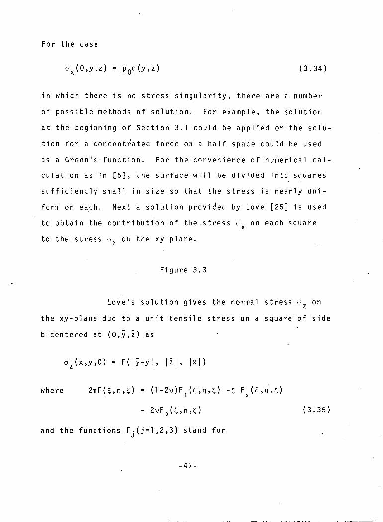
For the case

ffx(0,y,z) = pQq(y,z) (3.34)

in which there is no stress singularity, there are a number

of possible methods of solution. For example, the solution

at the beginning of Section 3.1 could be applied or the solu-

tion for a concentrated force on a half space could be used

as a Green's function. For the convenience of numerical cal-

culation as in [6], the surface w i l l be d i v i d e d into squares

sufficiently small in size so that the stress is nearly uni-

form on each. Next a solution provided by Love [25] is used

to obtain the contribution of the stress a on each squareA

to the stress a on the xy plane.

Figure 3.3

Love's solution gives the normal stress a on

the xy-plane due to a unit tensile stress on a square of side

b centered at (0,y,z) as

az(x,y,0) = F(|y-y| ,

where 2irFU,n,c) = (1-2v)Fi (?,n,c) -C F^C.n.c)

- 2vF3U,n,c) (3.35)

and the functions F.(j=l,2,3) stand forsJ

-47-

IS

Fo =b-n b+n

2 (b-n)2+?2 a: (b+n)2+?2 2(3.36)

F3 tan-1

+ tan

+ tan

+ tan2ir, |cl<b, |n|<b

0, otherwise

with the following contractions

2 _ + (b-n)2 +

(b+n)

+ ?

2 I -r 2

dj = (b-?)2 + (b+n)2 + c2

By taking advantage of symmetry, attention may

be confined to the centers (0 , y • , z •) of the squares which lie

in the first quadrant of the yz-plane. The effect of the

other three symmetrically located quadrants is i n c l u d e d in

the result

o,(x,y,0) = pnt(x,y)

where

0

N Nt(x,y) = 2 I I q(yi,i,)[F(|yry|,|z |, |x|)

i=l j=l J J

(3.37)

-48-

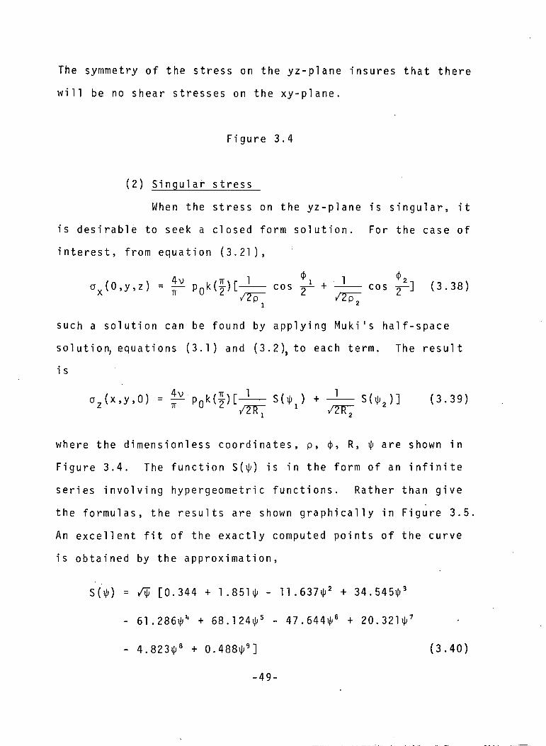
The symmetry of the stress on the yz-plane insures that there

w i l l be no shear stresses on the xy-plane.

Figure 3.4

(2) Singular stress

When the stress on the yz-plane is singular, it

is desirable to seek a closed form solution. For the case of

interest, from equation (3.21),

ox(0,y,z) = P0k(f)[-L- cos + -J— cos Ji] (3.38)X IT 0 2 2 - 2

such a solution can be found by applying Muki's half-space

solution, equations (3.1) and (3. 2 )} to each term. The result

i s

o_(x,y,0) = P0k(f)[-l— SU ) + -1— S(^)] (3.39)Z TT 0 2 -- -

where the dimensionl ess coordinates, p, 4>, R, ty are shown in

Figure 3.4. The function S(T(J) is in the form of an i n f i n i t e

series i n v o l v i n g hypergeometri c functions. Rather than give

the formulas, the results are shown graphically in Figure 3.5

An excellent fit of the exactly computed points of the curve

is obtained by the approximation,

' •? [ 0 . 3 4 4 + 1.851^ - 11.637i|j2 + 3 4 . 5 4 5 ^ 3

61.286i|>" + 6 8 . 1 2 4 ^ 5 - 47 .644 i^ 6 + 20.32H7

+ 0.488i|)9] (3.40)

-49-

This exp ress i on is va l i d only for 0_<<jK7r/2 and for P o i s s o n ' s

rat io, v = 0 .30.

Fi gure 3.5

It should be noted that there are singulari-

ties in a (x,y,0) at the points where the crack front inter-

sects the free surface. The numerical difficulties due to

the singularity w i l l be discussed in more detail in Section

3.4.

3.3 Iterative Formulation

The solutions of the two preceding problems w i l l

be superposed alternately to solve the case of a uniformly

pressurized half penny-shaped crack perpendicular to a free

surface (Figure 3.6). The procedure begins with the well

known solution [26] for uniform pressure of a penny-shaped

crack in an infinite medium. This solution gives stresses on

the yz-plane which are removed by superposing the half space

solution for equal and opposite stresses on the yz-plane.

As a result of the half space solution, there is a residual

normal stress on the crack in addition to the uniform pres-

sure. This is eliminated by superposing the solution of

Section 3.1 for pressure on the crack equal to the residual

stress. Again, stresses on the yz-plane are produced which

are removed by appl i c a t i o n of the half space solution. The

cycle of superpositions is continued until the resudual stress

on the crack is negligible compared to the uniform pressure.

-50-

Figure 3.6

As outlined, the first step in the procedure re-

quires the solution of the penny-shaped crack problem for the

case

a^fx.y.O) = -p0 (3.41)

Either [26] or Section 3.1 may be used to find the stress

intensity factor,

and the stress on the yz-plane,

a j v ( 0 , y , z ) = -p- p n k ( ° ' ( £ ) [ cos ^ + cos ^-JXM 71 U c r= c. m c.

/2p /2pi 2

+ P0q(0)(y,z) (3.43)

See Figure 3.4 for the coordinates, p,4>. For the case of(r\\ y

uniform pressure, qv (y,z) is equal to — FQ(y,z) which is

given in equation (3.28).

The second half of the zeroth iteration is used to

eliminate the stress on the free surface. The stress applied

to the surface is

ajSÔ.y.z) = aJJÔ.y.z) (3.44)AD A tt

which gives the result (See Figure 3.4 for R,^.)

1 2 (3.45)

-51-

where t^ (x,y) is determined by applying the method of

dSection 3.2(1). It depends only on q^ , and not on the

singular part of oA i \

After the second half of this iteration is sub-

tracted from the first half, the surface will be free of

stress, but the stress on the crack w i l l be

az(x,y,0) = -p0 - a^)(x,y,0) (3.46)

rather than constant. An additional iteration is used to

eliminate the stress o^ .

For the first iteration, the stre.ss on the penny-

shaped crack is taken to be

'/zirr /2trA O2

P0t(1)(x,y) (3.47)

Because of the singularity in the first term of equation

(3.47), care must be taken in the numerical procedure. The

description of the numerical method w i l l be given in the

following section. The contribution of the two parts of

a a are computed separately and the desired quantities ex-

pressed as

kO)(e) *£>. k(0>(£)Me) + k^(e) (3.48)

Tr £ o ii

q(1)(Y,z) = k(0)(f)qs(y,z) + q(1)(y,z) (3.49)TT e. * N

-52-

+ P 0 q ( 1 ) ( y , z ) ( 3 . 5 0 )

where k s ( 9 ) and p Q q s ( y , z ) are the d imension! ess s t ress inten-

sity factor and r ionsingular part of a ( 0 , y , z ) , respec t i ve l y ,/\

due to stress on the crack of

S( ) SU )sz(x,y,0) = pQ[ - + - — ] (3.51)2 u ~

Similarly, kl '(6) and p^qi (y,z) stem from the stress

Pt (x,y) on the crack.

The effects of these two terms are kept separate

into the second half of the iteration. The stress on the

half space is taken to be

This results in the residual stress on the crack,

(3.52)

where

t (2)(x,y) = k < ° ) t ( x , y ) + t ( x , y ) (3.53)

In a way similar to the definitions of q$ and q* ', t$ and

t,, ' are defined to be the stress a,(x,y,0) due to the stressz

-53- .

a (0,y,z) equal to q~ and q.;, ', respectively, and are foundX o IN

by the method of Section 3.2(1).

Again, the second half of the iteration when sub-

tracted from the first half frees the surface of stresses.

Adding the first iteration to the zeroth cancells the re-

sidual stress 0^0 and gives

tfz(x,y,0) = -p0 - a*BMx,y,0)

Further iterations are added until the stress on

the crack is reduced to the applied stress -PQ to within

some arbitrary tolerance. The additional computations which

must be made for each iteration are straightforward. For

the second iteration, the dimensionless intensity factor,(2) (2}kj, '(8), and stress a (0,y,z) = P QpM (y>z) due to stress on

(2}the crack of a (x,y,0) = p Qtv '(x,y) are obtained. Then the

half space solution gives a (x,y,0) = Pntl (x,y) due to(2)o" (0,y,z) = Ppo,,:, (y,z). The contribution of this iteration

X U IN

to the dimensionless stress intensity factor is

and the stress on the crack is

az(x,y,0) = -p

where

-54-

t(3)(x,y) =

For the n— iteration, the functions, ks(0),

q$(y»z)» and t<j(x,y), are used again in conjunction with

the results of the previous iteration, k^ n~ '(0) and

t (x,y). The method of Section 3.1 gives the new functions,

k^n'(0) and q^n'(y,z), which are, respectively, the dimen-

sionless stress intensity factor and the nonsingular part

of a (0,y,z) produced by application of the stress a (x,y,0)=f\ L-

t (x,y) to the crack. The half space solution of Section

3.2(1) gives tln+ ' (x ,y) , the stress a (x,y,0) produced by

a (0,y,z) = qin^(y,z) acting on the surface. The new addi-A ill

tion to the dimensionl ess stress intensity factor is

k(n)(e) = iv.k(n-l)(!.)ks(e) + k(n)(e)

and the residual stress on the crack is

0Oj>(x.y.O) . |i P k(»)(J)[ii!il +ZB TT 0 ^

where the term carried into the next iteration, if necessary,

is

The alternating method applied in this Section is

modified by the separate treatment of the singular part of

the stress (equation (3.43)) applied to the half space. The

solution for the half space subjected to the singular stress-55-

is given by the first part of equation (3.45). The

resulting stress which must be removed from the crack, eq.

(3.47), has two parts which are kept separate. The singular

part is the same in each iteration except for the coefficient

involved. Therefore, the numerical solution for a penny-

shaped crack subjected to the singular stress (tensile) of

equation (3.51) is determined to as high a degree of accuracy

as possible. The contribution of this solution to each

iteration is contained in the functions with a subscript, S.

The remaining contribution, from the rest of equation (3.47)

gives the terms denoted by the subscript, N. The parts are

combined as in equations (3.48) to (3.50) to give the total

solution of the penny-shaped crack problem for this iteration

The solution is treated by the same method in each successive

i teration.

The next section contains a description of the

numerical details and the difficulties associated with the

stress singularity of equation (3.47).

3.4 Numerical Treatment of Si ngularlties

(1) Half space

For the case of uniform pressure on the crack,

the first step requiring numerical analysis is the clearing

of the stress, eq.(3.43) from the surface in the second half

of the zeroth iteration. For convenience the problem is a

half space with tensile stresses,

ax(0,y,z) = pQq(y,z)

-56-

on the surface. The function q(y,z) can be any of the non-

singular functions of the first line of Table II. The solu-

tion for the singular part of the stress a (0,y,z) is givenX

analytically by equations (3.38) to (3.40).

The surface of the half space is divided into

a number of regions as shown in Figure 3.7. Each region is

then s u b d i v i d e d into a number of squares, larger squares

being used where the stress becomes small and less rapidly

varying. The values of q (y^z) at the centers of each of

the squares are computed from the closed form expression,

equation (3.28). Because of the lengthy calculations needed

to obtain the values of the other q's, they were computed

at fewer points and the six point bivariate interpolation

formula was used to get the values at the remaining points.

The numbers in parentheses in Figure 3.7 give the number of

values of y and the number of values of z, respectively, used

to obtain the grid points at which q was calculated exactly.

After the values of q(y,z) have been computed at the center

of each square, the solution in Section 3.2(1) is used

directly to obtain the values of the stress on the xy-plane

denoted by

crz(x,y,0) = p0t(x,y) (3.54)

where the t's corresponding to the various q's are shown in

Table II.

-57-

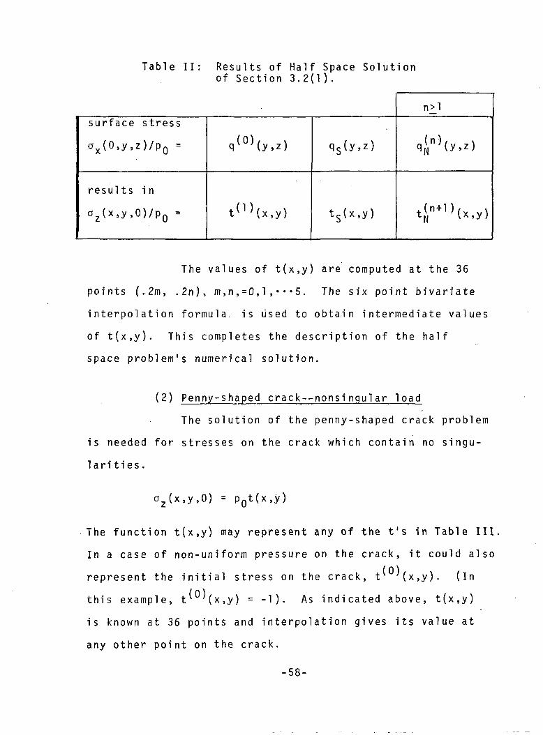
Table II: Results of Half Space Solutionof Section 3.2(1).

surface stress

ax(0,y,z)/pQ =

results in

oz(x,y,0)/pQ =

q(0)(y,Z>

t«'(*,y>

qs(y,z)

t$(x,y)

n>l

qN ^y 'z '

t<"+1)(x,y)

The values of t(x,y) are computed at the 36

points (.2m, .2n), m,n,=0,l,*«*5. The six point bivariate

interpolation formula is used to obtain intermediate values

of t(x,y). This completes the description of the half

space problem's numerical solution.

(2) Penny-shaped crack--nonsi ngul ar loag^

The solution of the penny-shaped crack problem

is needed for stresses on the crack which contain no singu-

larities.

az(x,y,0) = pQt(x,y)

The function t(x,y) may represent any of the t's in Table III

In a case of non-uniform pressure on the crack, it could also

represent the i n i t i a l stress on the crack, t* (x,y). (In

this example, t' ^(x,y) = -1). As indicated above, t(x,y)

is known at 36 points and interpolation gives its value at

any other point on the crack.

-58-

The solution of Section 3.1 requires first the

computation of the Fourier coefficients of

P(r,e) = -t(x,y)

which areTT/2

K0(r) = | | p(r,6)d0

0TT/2

K2m(r) = 1 | p(r,6)cos2mede, mH (3.55)0

K2m+1(r) = 0 , m>0

The first 40 K's are each computed for 30 values of r using

a technique given by Filon [27]. His technique gives as

good accuracy with 100 d i v i s i o n s of the range of integration

as the usual Simpson's rule does with 500.

The coefficients of a five term polynomial

approximation to each K are determined by the method of

least squares. This gives

W"' ' ,*.*! .i.r" ' "i1 (3'56)

where A , m=l ,2, • • «40; n = l,2,-"5 are known constants and

p =p(0,9). The polynomial form of the K's enable gm(t) to beO III '

determined also in polynomial form as in equation (3.24),

-59-

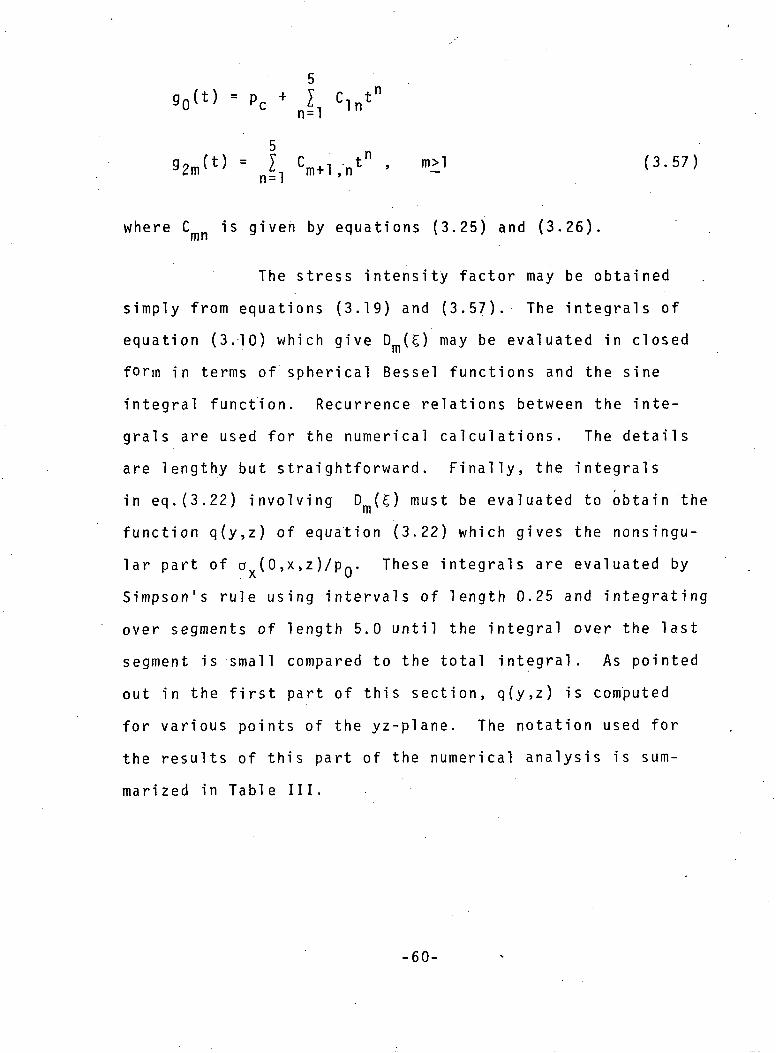
9°(t) =

j, V'."*" ' "i1 '3'57)

where C is given by equations (3.25) and (3.26).

The stress intensity factor may be obtained

simply from equations (3.19) and (3.57). The integrals of

equation (3.10) which give D (£) may be evaluated in closed

form in terms of spherical Bessel functions and the sine

integral function. Recurrence relations between the inte-

grals are used for the numerical calculations. The details

are lengthy but straightforward. Finally, the integrals

in eq.(3.22) in v o l v i n g Dm(£) must be evaluated to obtain the

function q(y,z) of equation (3.22) which gives the nonsingu-

lar part of a (0,x,z)/pQ. These integrals are evaluated by

Simpson's rule using intervals of length 0.25 and integrating

over segments of length 5.0 until the integral over the last

segment is small compared to the total integral. As pointed

out in the first part of this section, q(y,z) is computed

for various points of the yz-plane. The notation used for

the results of this part of the numerical analysis is sum-

marized in Table III.

-60-

Table III: Stress Intensity Factors and Stresseson yz-Plane for Various Loads on Crack.

stress on crack

tfz(x,y,0)/p0 =

produces stress°x(0,y,z)/p0whose nonsing.part is =

produces stressintensity factor

kp(6)/| P0/a =

eq.(3.51)/p0

qs(y,z)

ks(e)

t(0)(x,y) = -1

q(0)(y,z) =

IF0^'2)(see eq. (3.28)

kt°)(6) = 1

n l

t(n)(x,y)

qSn)(y.i)

k^n)(e)

For n>2, t(n)(x,y) = k(n'2 } (f)ts(x ,y ) + t<n)'(x,y) (See T.II)

For n>l, k< n>(e) = k( > (|) ks(6) + 4 (0)

( 3 ) Penny-shaped crack -- singular load

The singular stress on the crack was given in

equation (3.39). For the numerical analysis consider the

dimensionless form,

Note that since a >0, the singular part of the load on the -

crack gives a negative stress intensity factor. Further,

since larger tensile stresses occur near'the intersection of

-61-

the crack front with the surface, the stress intensity factor

should be expected to be larger in magnitude there. Thus,

when combined with the other contributions to the stress in-

tensity factor, this w i l l cause a decrease in the total as

the surface is approached.

Because of the singularity, it would be advantageous

, to have a closed form solution for this part of the problem.

But since none could be found, it was decided to use the same

numerical method given for nonsingular loads. It is evident

that more terms and finer mesh sizes are required. Limita-

tions on computer time forced the use of the same number of

points in r and the same number of terms in the r expansion

as above. More terms were included in the Fourier series,

and smaller s u b d i v i s i o n s were used in the integration. It

was found that KM) decreased very slowly as m increased.

For m=400, Km(l) was of the order of 10"2, Km(.967), of 10"3,

Km(.933), of 10"4, and for r<.5, Km(r) was of the order 10~

5.

For m=1600 these figures decreased by a factor of 10. Each

time additional terms were included in the Fourier series,

the magnitude of k<.(6), the dimensionl ess stress intensity

factor due to the singular pressure on the crack, increased

near 9 = ir/2 and remained the same elsewhere. Finally ks(e)

was calculated using 841 terms in the cosine series.

The function q.(y,z) which gives the nonsingular part

of the stress a (0,y,z) due to the load on the crack/\

-62-

was .computed using 241 terms in the Fourier series. This

part of the numerical solution required more than half of

the computer time used. But note that the same function

is used again in each iteration.

In reference [6] which also treats this pro-

blem there is no separation of singular and nonsingular

terms in the numerical analysis. The half space problem

utilizes stresses at points within Regions I and III of

Figure 3.6. Outside these regions, the stress is approxi-

mated by zero. In [6], the stress is computed at 80 points

within Region I, as compared with 45 in this analysis. The

additional points should not be expected to account accurately

for the singularities.

To obtain the stresses in the regions mentioned

above and to obtain the stress intensity factor for a given

stress on the penny shaped crack in [6], the stress on the

crack is computed for five values of r and 19 values of 0.

Weddle's rule is applied to the integrals for K (r) for

m=0,2,4,•••10. Simpson's rule using, say, 40 values of 6

should be as accurate. Km(

r) 1S obtained in [6] as a fifth

order polynomial in r by forcing the polynomial to pass

through the computed points. In this work, Km(r) is known

at 30 values of r, and the fifth.-order polynomial is obtained

by least squares curve fitting.

-63-

3.5 Discussion of Numerical Results

The result.of the analysis described above is the

curve in Figure 3.8. which shows the variation of the stress

intensity factor along the crack front. The deepest point of

the crack is 6=0. Initially, moving away from this point,

there is a gradual increase in stress intensity factor. Then

about 20° from the surface there is a rapid increase. Fol-

lowing this a more rapid decrease occurs in the last 3°.

Note that the. stress,intensity factor tends to zero at the

surface, a result discussed in several previous papers [22,

28,29], It appears that an increase in numerical accuracy

would further decrease the value at the surface toward zero.

However, the lack of an exact solution of the problem of a

crack loaded by the stress of equation (3.51) is reflected

by an accumulation of numerical inaccuracies as the number

of iterations is increased.

Figure .3.8

It should be clear that the results in Figure 3.8

are by no means the exact solution of the problem but are

presented as the best approximation available. The trend of

the curves differs substantially from those obtained in [6]

using basically the same numerical procedure. The results of

[6], shown as a dashed line in Figure 3.8, would be expected

to differ slightly from the present results because they were

-.64-

obtained for a Poisson's ratio of 0.25 and the present ones,

0.30. The apparent reason for the qualitative difference

between the results is the differing treatments of the sin-

gularities. As background information some intermediate

results w i l l be given.

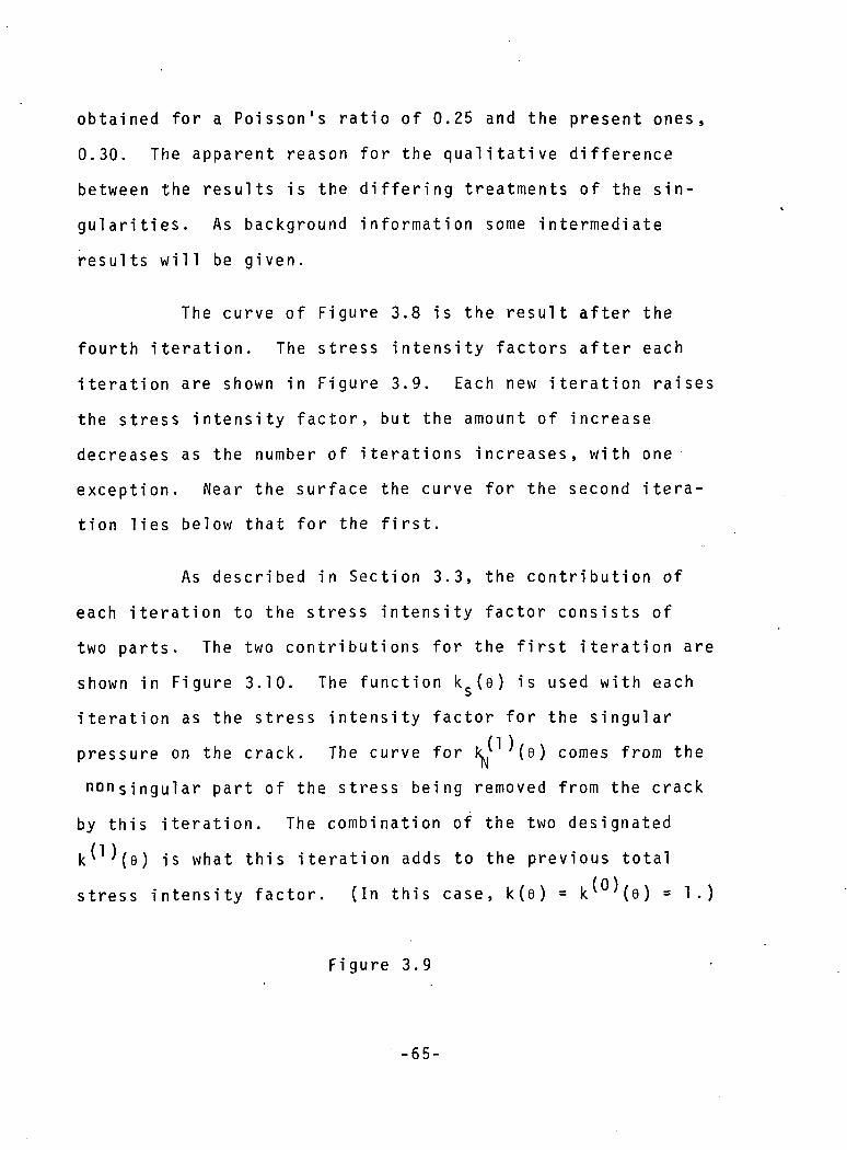
The curve of Figure 3.8 is the result after the

fourth iteration. The stress intensity factors after each

iteration are shown in Figure 3.9. Each new iteration raises

the stress intensity factor, but the amount of increase

decreases as the number of iterations increases, with one

exception. Near the surface the curve for the second itera-

tion lies below that for the first.

As described in Section 3.3, the contribution of

each iteration to the stress intensity factor consists of

two parts. The two contributions for the first iteration are

shown in Figure 3.10. The function ks(e) is used with each

iteration as the stress intensity factor for the singular

pressure on the crack. The curve for k* (e) comes from the

singular part of the stress being removed from the crack

by this iteration. The combination of the two designated

k^ '(0) is what this iteration adds to the previous total

stress intensity factor. (In this case, k(e) = k^ '(e) = 1.)

Figure 3.9

-65-

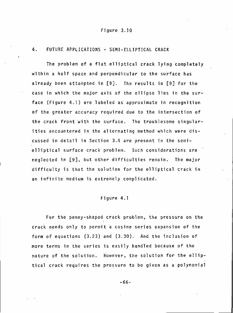
Figure 3.10

4. FUTURE APPLICATIONS - SEMI-ELLIPTICAL CRACK

The problem of a flat elliptical crack lying completely

within a half space and perpendicular to the surface has

already been attempted in [9]. The results in [9] for the

case in which the major axis of the ellipse lies in the sur-

face (Figure 4.1) are labeled as approximate in recognition

of the greater accuracy required due to the intersection of

the c.rack front with the surface. The troublesome singular-

ities encountered in the alternating method which were dis-

cussed in detail in Section 3.4 are present in the semi-

elliptical surface crack problem. Such considerations are

neglected in [9], but other difficulties remain. The major

difficulty is that the solution for the elliptical crack in

an infinite medium is extremely complicated.

Figure 4.1

For the penny-shaped crack problem, the pressure on the

crack needs only to permit a cosine series expansion of the

form of equations (3.23) and (3.30). And the inclusion of

more terms in the series is easily handled because of the

nature of the solution. However, the solution for the ell i p -

tical crack requires the pressure to be given as a polynomial

-66-

N MP(x.y) = I I a xray" (4.1)

n=0 m=0 mn

It is possible to work out the solution for any finite number

of terms of equation (4.1), although, for a large number, it

is impractical. Thus far, no way has been found to include

the effect of additional terms in (4.1) by a recurrence scheme.

The additional terms require the solution for the lower order

terms and additional contributions combined in a complicated

way.

As a result of the difficulty, the elliptical crack prob-

lem was restricted in [9] to be of the form

p(x.y) = aOQ + a01y + a2Qx2 + a02y

2 + a21x2y + aQ3y

3

(4.2)

The six constants in this equation are determined by a least

squares technique of fitting equation (4.2) to a number of

known values of p(x,y). The odd powers of x are omitted

because the problem is taken to be symmetric about the yz-

plane. For the e l l i p t i c a l surface flaw, the pressure would

also be made symmetric about the xz-plane, and the odd powers

of y would be eliminated. Thus, only three constants, a ,

a?0' an?' wou^ be a v a i l a b l e for the least square fitting

necessary. Additional terms are clearly needed, but the 200

terms used in the penny-shaped crack solution (40 in 6, 5 in r)

cannot be approached.

-67-

As suggested by Kantorovich and Krylov [2], the Schwarz-

Neumann Alternating Technique has wide applicability. It can

be applied to other three-dimensional crack problems of

interest such as the finite thickness crack problem. The

crack may be taken to intersect the plate at any angle. Such

problems would involve combined modes of crack extension even

though the plate is loaded in simple tension.

There is some arbitrariness in the choice of the two

sequences of problems involved in the alternating method. For

example, in Section 2.3, the stress, o(x), on the edge crack

was extended symmetrically to negative values of x in the

zeroth iteration. It would have been possible to make the

stress skew-symmetric about the y-axis instead. The two se-

quences of problems would then be quite different. Similarly,

in the surface crack problem, the i n i t i a l pressure on the

penny-shaped crack could be taken to be skew-symmetric about

the yz-plane. The problems which make up the two sequences

would then have different characteristics. In general, the

various alternatives should be studied to determine whether

one provides a better representation of the essential proper-

ties of the problem.

It is conceivable that in some applications the alter-

nating method w i l l involve three or more sequences of solu-

tions. In general, one sequence would be expected to be

necessary for each part of the boundary of the material.

-68-

If there were three parts of the boundary and three solutions,

the sequence would be formed similarly to the examples pre-

sented here. Each solution would produce some undesirable

residual stresses on the other two boundaries. Thus, each

iteration would use each solution in turn to remove the

residual stresses produced by the other two solutions in

their previous applications.

-69-

APPENDIX

Stress intensity factors for various particular loads

on the edge crack are listed here. For other loads the

general expression of eq.(2.50) may be used. In addition,

results for the penny-shaped crack in an infinite body are

given, i n c l u d i g g some recently published stress intensity

factors for non-axisymmetrically loaded cracks.

Edge Cracks

(1) Concentrated forces (Figure 2.4)

For concentrated normal and shearing forces applied

to the crack as shown in Figure 2.4, the stress intensity

factors are

K , "~ ~~~"1 TT /a2-b2

_ 2

v/a2-b2

where f(b/a) is given by equation (2.47) and Figure 2.5.

Figure A-l

(2) Linear stress (Figure A-l)

In this case, the stress on the crack varies linearly

from zero at the edge to twice the average stress at the

crack tip (Figure A-l). The stress intensity factors in

-70-

terms of the average stresses are

k = 1 .3660 a, /ai a

k, = 1 .3660 T, /a"^ a

Figure A-2

(3) Uniform stress near crack tip (Figure A-2)

As shown in Figure A-2, the crack is free of stress

on the part of its faces adjacent to the edge and is sub-

jected to uniform stresses on the other part up to the crack

tip. The stress intensity factors may be expressed as

k2 = | . a r ccos (b /a )T 0 / a [ l +h l ( b /a ) ]

where h^b/a) is shown in Figure A-3. These results may

also be expressed in terms of the average stresses on the

crack,

aa = (l-b/a)a0 Ta = (l-b/a)T0

The stress intensity factors

= h 2 ( b / a ) a a / a ~

k2 = h 2 ( b / a ) T a / a ~

-71-

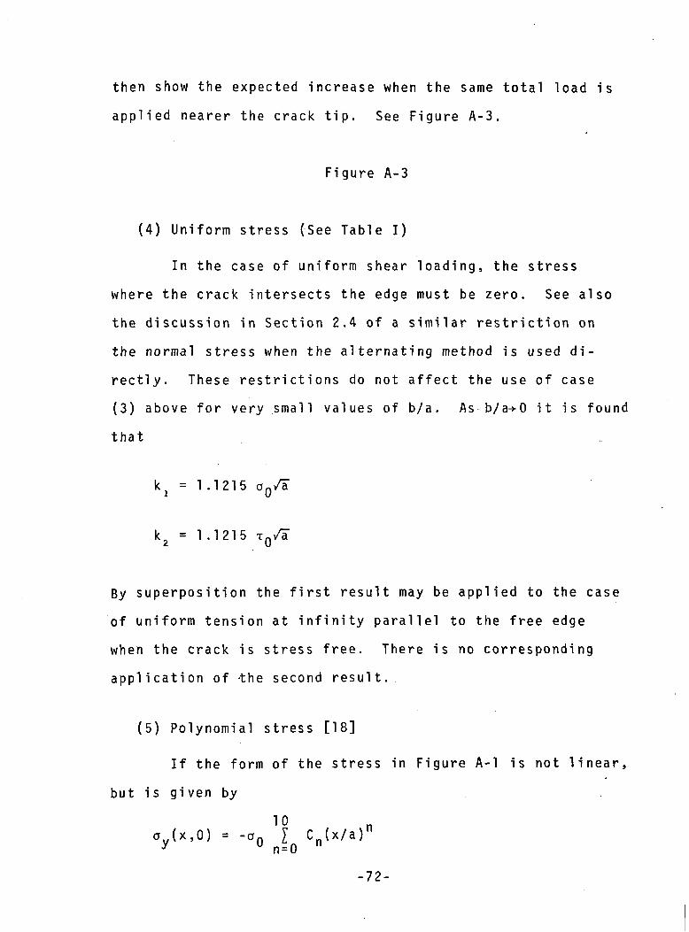
then show the expected increase when the same total load is

applied nearer the crack tip. See Figure A-3.

Figure A-3

(4) Uniform stress (See Table I)

In the case of uniform shear loading, the stress

where the crack intersects the edge must be zero. See also

the discussion in Section 2.4 of a similar restriction on

the normal stress when the alternating method is used di-

rectly. These restrictions do not affect the use of case

(3) above for very small values of b/a. As b/a-»-0 it is found

that

= 1 .1215 o0/a

k2 = 1 .1215 TQ/a

By superposition the first result may be applied to the case

of uniform tension at infinity parallel to the free edge

when the crack is stress free. There is no corresponding

application of -the second result.

(5) Polynomial stress [18]

If the form of the stress in Figure A-l is not linear,

but is given by

%(x'0) = -<*<, I C (x/a)ny u n=0 r

-72-

where C0, C , •••, CIQ are arbitrary constants, then the

stress intensity factor is [18]

kj = a0/2¥[0.7930C0 + 0.4829C1 + 0.3716C,, + 0.3118C3

+ 0.2735CU + 0.2464C, + 0.2260C. + 0.2099C,H o o /

+ 0.1968Cfl + 0.1858CQ + 0.1765C,Jo 9 '10

If there is shear loading T ' (x,0) given by the expressionxy

for a (x,0), but with aQ replaced by TQ, then by the state-

ment following eq.(2.50), the Mode II stress intensity

factor, k , is given by the expression for k with. an replaced2 1 •' U

by TO.

jênny-Shaped Cracks

(6) General result (Figure 3.1)

The pressure applied to the crack is in the form

a = -P0 I Km(r)cosme, z = 0,m=0

where r is the distance from the z-axis divided by the crack

radius, a. The resulting Mode I stress intensity factor is

= - pQ/a I g (l)cosme77 u m=0

where

-73-

These formulas apply only when the stress on the crack

is symmetric about a plane containing the z-axis (the 6=0

plane). For the special case of axisymmetric loading the

only nonzero Km(r) is KQ(r), and the equations simplify

considerably.

(7) Uniform tension (Figure A-4) [26]

By superposition, the stress intensity factor due to

the uniaxial tension may be determined by considering the

same geometry, but with uniform pressure,

az = ~aO ' z=0' r<1

on the crack and zero stress at infinity. For this problem

the parameters of case (6) are

P0 = aO ' K0(r) = ] ' Km(r) = °*

Therefore, the stress intensity factor is [26].

Figure A-4

(8) Uniform shear (Figure A-4) [30]

The solution in [30] for constant shearing stresses

on the faces of a penny-shaped crack may be used to obtain

the stress intensity factors for Figure A-4.

-74-

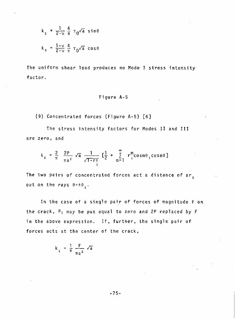
4 i—— Tn/a s i n e

cose

The uniform shear load produces no Mode I stress intensity

factor.

Figure A-5

(9) Concentrated forces (Figure A-5) [6]

The stress intensity factors for Modes II and III

are zero, and

k = - =2— /a —-— [4- + I r c o s m e . c o s i n e ]* Tra 2 /T^lrT ^ m=l J J

The two pairs of concentrated forces act a distance of art

out on the rays 0=±0i.

In the case of a single pair of forces of magnitude F on

the crack, 61 may be put equal to zero and 2P replaced by F

in the above expression. If, further, the single pair of

forces acts at the center of the crack,

l - L _ / a

• 7 5 -

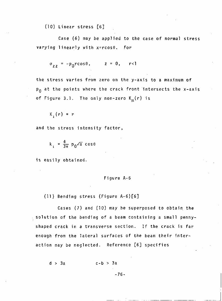
(10) Linear stress [6]

Case (6) may be applied to the case of normal stress

varying linearly with x=rcos0. For

a = -p0rcos9, z = 0, r<l

the stress varies from zero on the y-axis to a maximum of

P0 at the points where the crack front intersects the x-axis

of Figure 3.1. The only non-zero Km(r) is

K:(r) = r

and the stress intensity factor.

= P^ cose

is easily obtained.

Figure A-6

(11) Bending stress (Figure A-6)[6]

Cases (7) and (10) may be superposed to obtain the

solution of the bending of a beam containing a small penny-

shaped crack in a transverse section. If the crack is far

enough from the lateral surfaces of the beam their inter-

action may be neglected. Reference [6] specifies

d > 3a c-b > 3a

-76-

where the dimensions of the beam are shown in Figure A-6.

An additional restriction must be placed on the dimensions

to insure that the crack faces are not compressed together,

for the solution would be i n v a l i d if that happened. This

restri ction,

b > f a

simply makes the stress intensity factor positive at all

points of the crack front. In terms of the moment of inertia,

I = 2dc3/3, of the cross-section, the stress produced in an

uncracked beam is

MQaa = —y— (b/a - rcose), z = 0, r<l

By superposition, the stress intensity factor

7 Mnaki = f -f- S* (b/a - (2/3)cos6)

may be found by considering the beam to be loaded only by

stresses on the faces of the crack equal and opposite to those

produced in the uncracked beam.

Surface Crack

(12) Uniform stress

The geometry of the half penny-shaped crack at the

surface of a half space is shown in Figure 3.6. For the case

of uniform tension at infinity perpendicular to the crack

(or uniform pressure on the crack faces), the stress inten-

sity factor is given in Figure 3.8.-77-

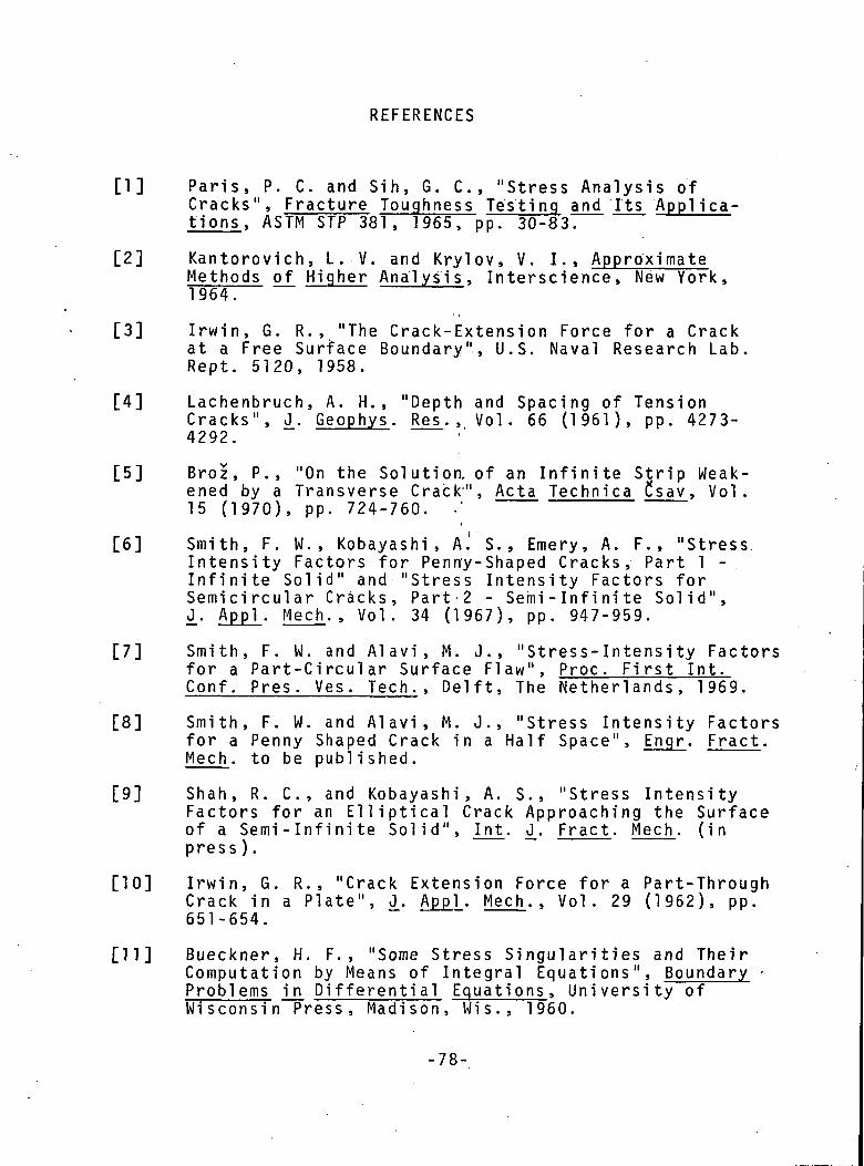
REFERENCES

[I] Paris, P. C. and Sih, G. C., "Stress Analysis ofCracks", Fracture Toughness Testing and Its Applica-tions. ASTM STP 381, 1965, pp. 30-83.

[2] Kantorovich, L . - V . and Krylov, V. I., ApproximateMethods of Higher Analysis, Interscience, New York,1964.

[3] Irwin, G. R. , "The Crack-Extension Force for a Crackat a Free Surface Boundary", U.S. Naval Research Lab.Rept. 5120, 1958.

[4] Lachenbruch, A. H., "Depth and Spacing of TensionCracks", J_. Geophys. Res. , Vol. 66 (1961), pp. 4273-4292.

[5] Broz, P., "On the Solution, of an Infinite Strip Weak-ened by a Transverse Crack1", Acta Technica Csav, Vol.15 (1970), pp. 724-760. .'

[6] Smith, F. W. , Kobayashi , A.' S. , Emery, A. F., "StressIntensity Factors for Penny-Shaped Cracks, Part 1 -Infinite Solid" and "Stress Intensity Factors forSemicircular Cracks, Part'2 - Semi -Infinite Solid",J.. Appl . Mech. . Vol. 34 (1967), pp. 947-959.

[7] Smith, F. W. and A l a v i , M. J., "Stress-Intensity Factorsfor a Part-Circular Surface Flaw", Proc. First Int.Conf. Pres. Ves. Tech. . Delft, The Netherlands, 1969.

[8] Smith, F. W. and A l a v i , M. J., "Stress Intensity Factorsfor a Penny Shaped Crack in a Half Space", Engr. Fract.Mech. to be published.

[9] Shah, R. C., and Kobayashi, A. S., "Stress IntensityFactors for an Elliptical Crack Approaching the Surfaceof a Semi -Infinite Solid", Int. J^. Fract. Mech. (inpress).

[10] Irwin, G. R. , "Crack Extension Force for a Part-ThroughCrack in a Plate", ^. Appl. Mech.. Vol. 29 (1962), pp.651-654.

[II] Bueckner, H. F. , "Some Stress Singularities and TheirComputation by Means of Integral Equations", Boundary -Problems in Differenti al Equations, University ofWisconsin Press, Madison, Wis., 1960.

-78-

[12] Winne, D.H. and Wundt, B.M., "Application of theGriffith-Irwin Theory of Crack Propagation to theBursting Behavior of Disks, Including Analyticaland Experimental Studies", Trans. ASME, Vol. 80(1958), pp. 1643-1655.

[13] Koiter, W.T., discussion of paper by Bowie, J. Appl.Mech., Vol. 32 (1965), p. 237.

[14] Koiter, W.T., "On the Flexural Rigidity of a BeamWeakened by Transverse Saw-Cuts", Proc. Kon. Ned.Akad. Wet.. (B), Vol. 59 (1956), pp. 354-374.

[15] Sneddon, I.N., Fourier Transforms, McGraw-Hill,New York, 1951.

[16] Wiggleswort«h,L .A. , "Stress Distribution in a NotchedPlate", Mathematika. Vol. 4 (1957), pp. 76-96.

[17] Doran, H.E., and Buchwald, V.T., "The Half-Plane withan Edge Crack in Plane Elastostatics", J_. Inst. Maths.Applies. . Vol. 5 (1969), pp. 91-112.

[18] Stallybrass, M.P., "A Crack Perpendicular to anElastic Half-Plane", Int. J_. Engr. Sci . , Vol. 8(1970), pp. 351-362. ;

[19] Sneddon, I.N. and Das, S.C., "The Stress IntensityFactor at the Tip of an Edge Crack in an ElasticHalf Plane", Int. J. Engr. Sci., Vol. 9 (1971),pp. 25-36.

[20] Magnus, W. and Oberhettinger, F., Formulas and Theoremsfor the Functions of Mathematical Physics, Chelsea,New York, 1949.

[21] Sih, G.C. and Liebowitz, H., "Mathematical Theoriesof Brittle Fracture", Fracture, Vol. 2, AcademicPress, New York, 1968.

[22] Sih, G.C., "A Review of the Three-Dimensional StressProblem for a Cracked Plate", Int. J_. Fract. Mech.Vol. 7 (1971 ), pp. 39-61.

[23] Thresher, R.W. and Smith, F.W., "Stress IntensityFactors for a Surface Crack in a Finite Solid"ASME Paper No. 71-APMW-6, J_. Appl . Mech. , in press.

[24] Muki, R.} "Asymmetric Problems of the Theory ofElasticity for a Semi-Infinite Solid and a ThickPlate", Progress in Solid Mechanics, Vol. 1.,North-Holland P u b l i s h i n g Co., Amsterdam, 1960,pp. 401-439.

-79-

[25] Love, A.E.H., "The Stress Produced in a Semi-InfiniteSolid by Pressure on Part of the Boundary", Phil.Trans. Roy. Soc. (A), Vol. 228 (1929), pp. 377 20.

[26] Sneddon, I.N., "The Distribution of Stress in theNeighbourhood of a Crack in an Elastic Solid", Proc.

• Roy. Soc. (A), Vol. 187 (1946), pp. 229-260.

[27] Filon, L.N.G., "On a Quadrature Formula for Trigon-ometric Integrals", Proc. Roy. Soc. Edin. , Vol. 49(1928-29), pp. 38-47.

[28] Hartranft, R.J. and Sih, G.C., "The Use of Eigenfunc-tion Expansions in the General Solution of Three-Dimensional Crack Problems", J. Math. Mech., Vol. 19(1969), pp. 123-138.

[29] Sih, G.C., W i l l i a m s , M.L., Swedlow, J.L., "Three-Dimensional Stress Distribution Near a Sharp Crack ina Plate of Finite Thickness", Air Force MaterialsLaboratory, Wright-Patterson Air Force Base, November1966 (AFML-TR-66-242).

[30] Segedin, C.M., "Note on a Penny-Shaped Crack UnderShear", Proc. Camb. Phil . Soc. . Vol. 47 (1951),pp. 396-400.

-80-

Fig. 2.1: Edge-cracked plate

-81-

oy(x.O) = -q(x)

-S

Fig. 2.2: Cracked infinite plate

-82-

ay(x,0) = p(x)

Fig. 2.3: Edge-loaded half plane

-83-

Fig. 2.4: Concentrated forces on an edge crack

-84-

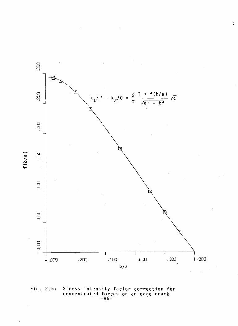
oo

oU3Csl

DoCM

(O LD

OCD

O

-.oca .200 .4DO I -QDG

b/a

Fig. 2.5: Stress intensity factor correction forconcentrated forces on an edge crack

-85-

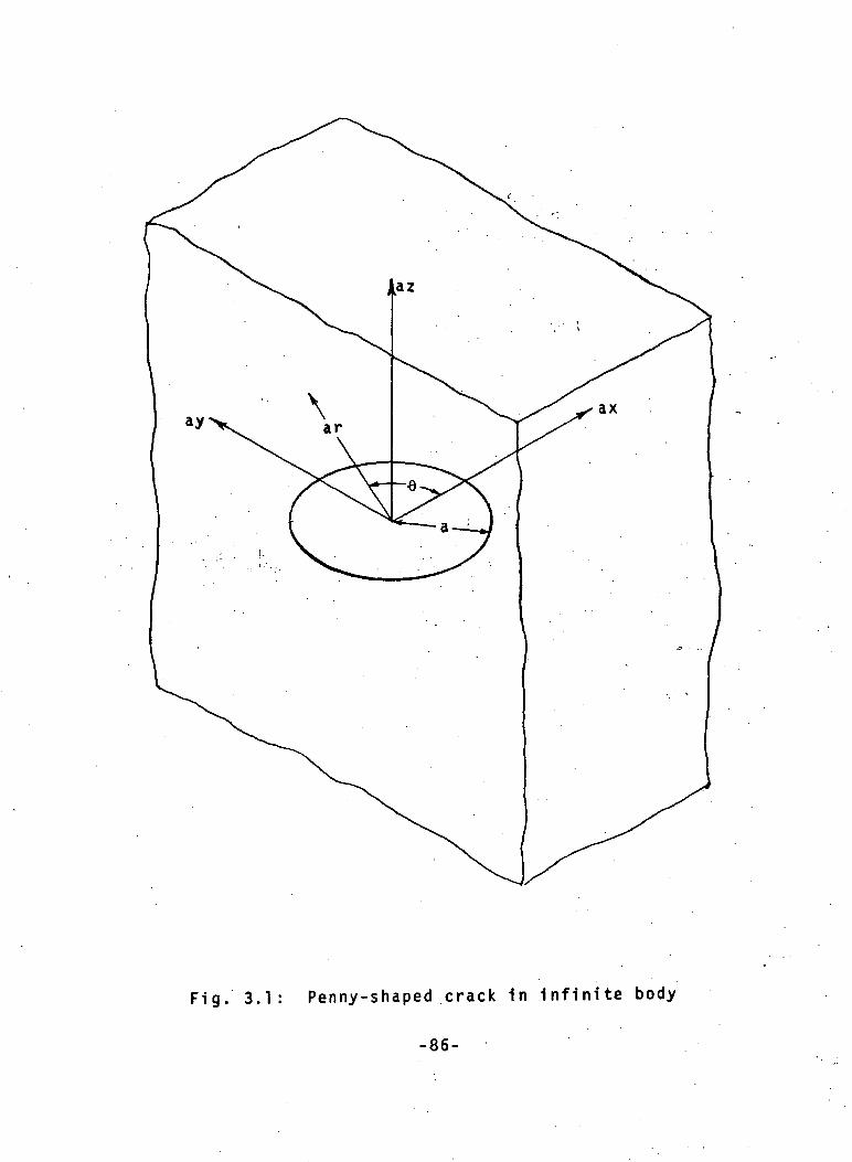
Fig. 3.1: Penny-shaped crack in infinite body

-86-

crack front

Fig. 3.2: Local coordinates (p,<f>) at crack front

-87-

Fig. 3.3: Half space (x £ 0) loaded on surface (x = 0)

-88-

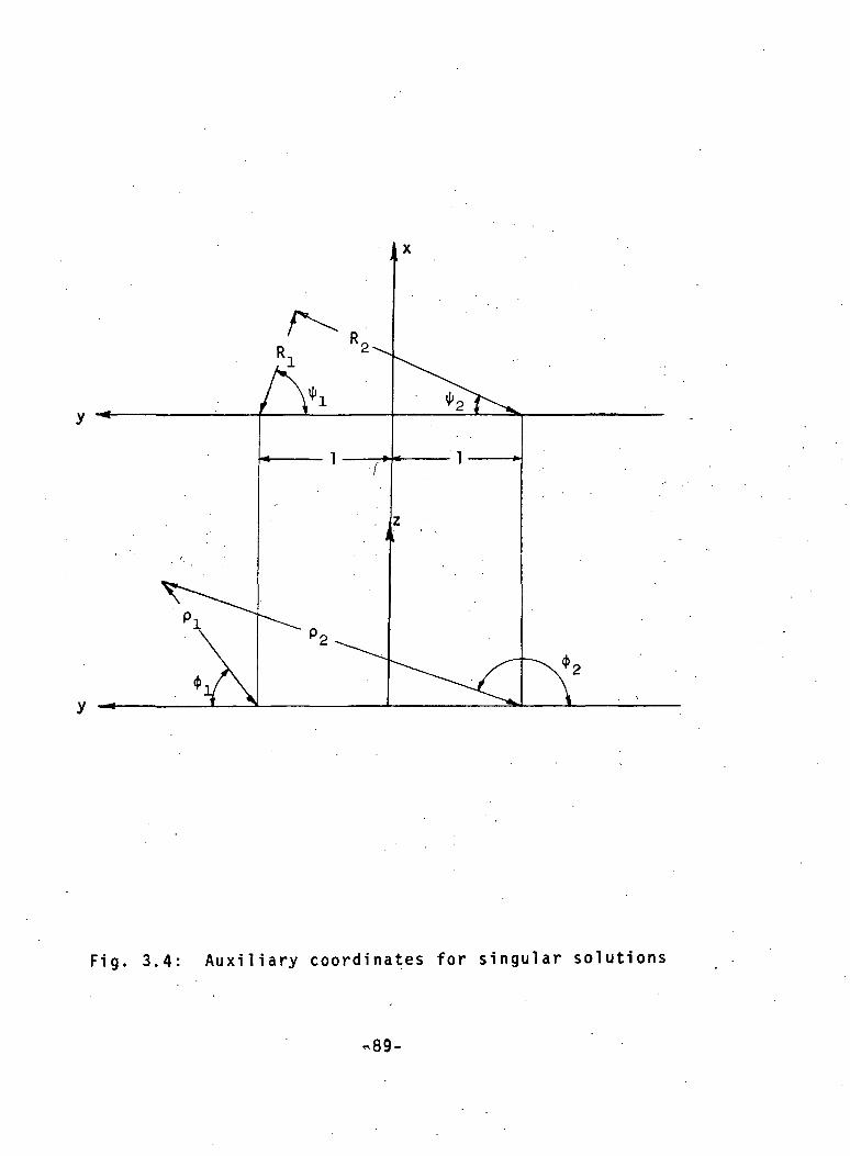
R 2Rl

1 r*

Fig. 3.4: Auxiliary coordinates for singular solutions

-89-

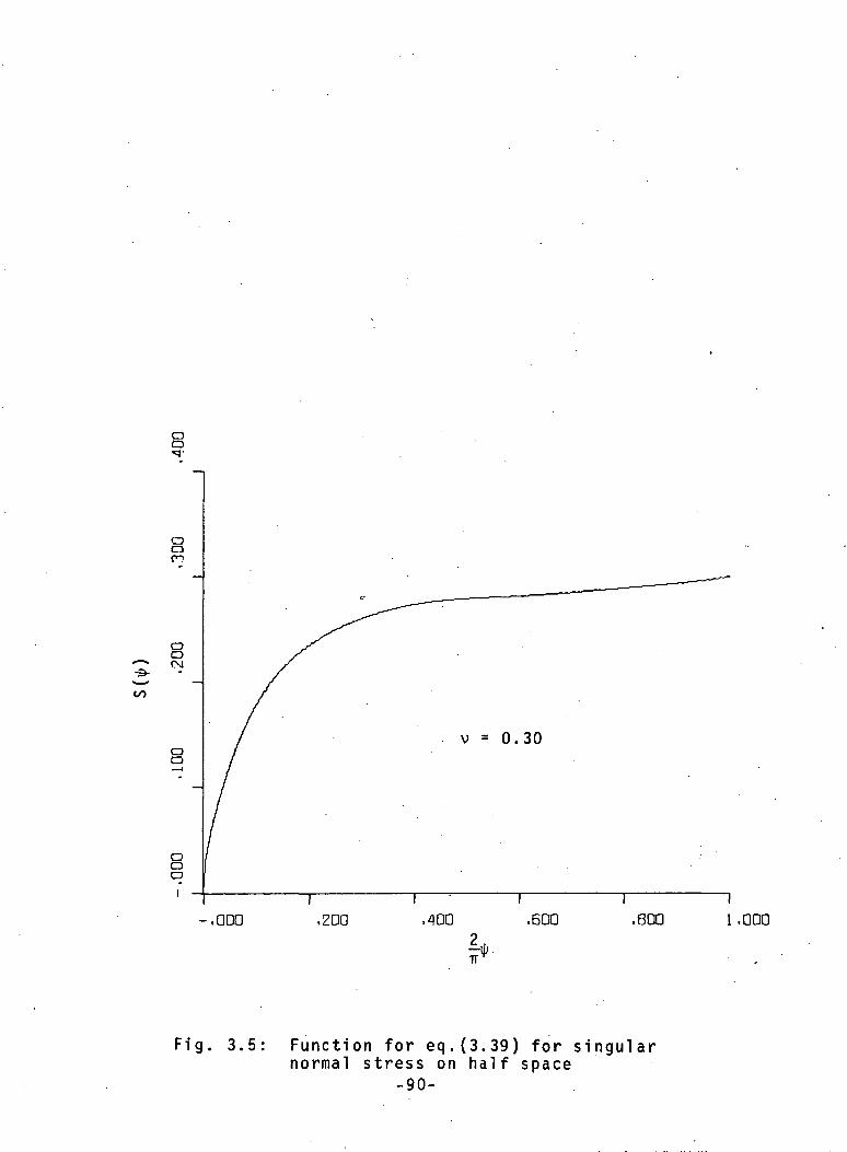
ooen

ooCM

ao

ooo

-.ODD ,200

v = 0.30

1 1 1 1 1,400 ,600

I*-.800 1 .000

Fig. 3.5: Function for eq.(3.39) for singularnormal stress on half space

-90-

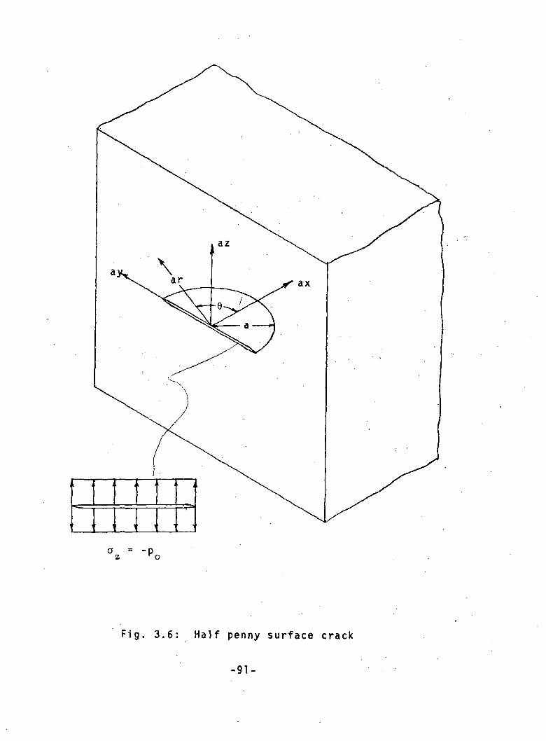
a = -pz r

Fig. 3.6: Half penny surface crack

-91-

(3,5)

VI

144 squares

(3.3)

V

100 squares

(3,3)

25

(4,3)II 75

(3,4)

III

150

(9,5)I 1250

Fig. 3.7: Grid on surface of half space

-92-

1.25-

1.20--

1.15-

CD

1.10-

1.05

1.00

Prom Section 3.5(v = 0.30)

From Ref. [6](v = 0.25)

Fig. 3.8: Stress intensity factor for Fig. 3.6

-93-

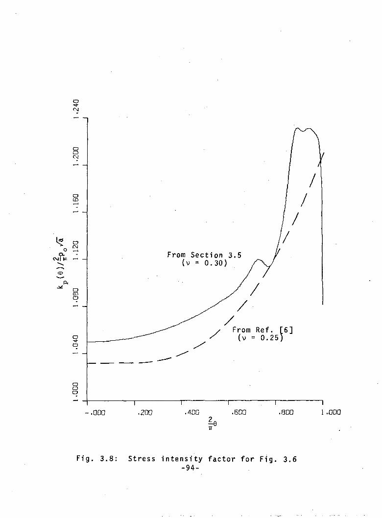
0-<*•(M

OOCN!

oto

CD

OCOo

D•<*•O

From Section 3.5(v = 0.30)

From Ref. [6](v = 0.25)

— I — I I . I I-.000 .200 .400 .600 .800 1.000

ie7T

Fig. 3.8: Stress intensity factor for Fig. 3.6-94-

o-*Csl

O

-.ODD .QDQ

Fig. 3.9: Successive iterations for thestress intensity factor

-95-

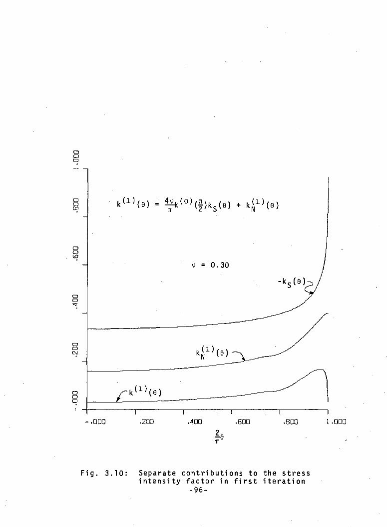
ooo

-.ODD ,2QO ,400 ,600 .800I1 .000

Fig. 3.10: Separate contributions to the stressintensity factor in first iteration

-96-

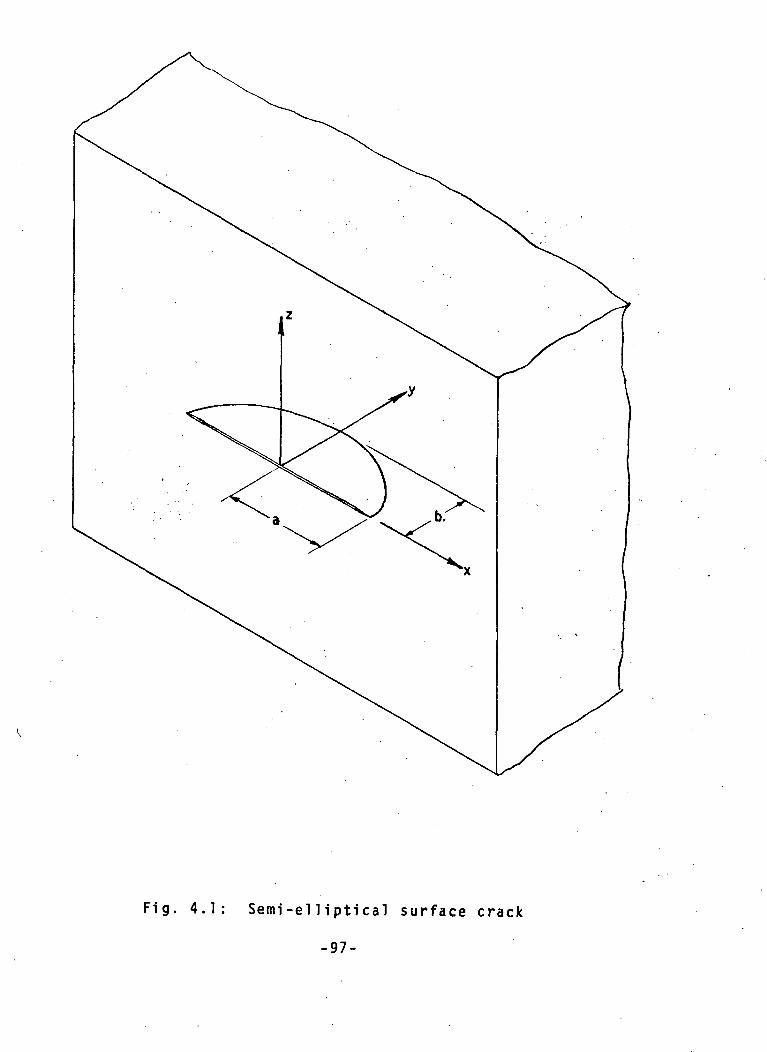
Fig. 4.1: Semi-el 1iptical surface crack

-97-

oy(x.O)

X.a

Fig. A-l : Linearly loaded edge crack

-98-

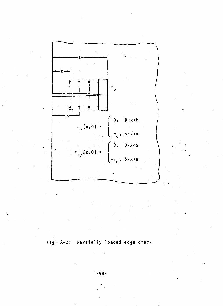
a (x,0) =0, 0<x<b

-aQ, b<x<a

6, 0<x<b

-T , b<x<ao

Fig. A-2: Partially loaded edge crack

-99-

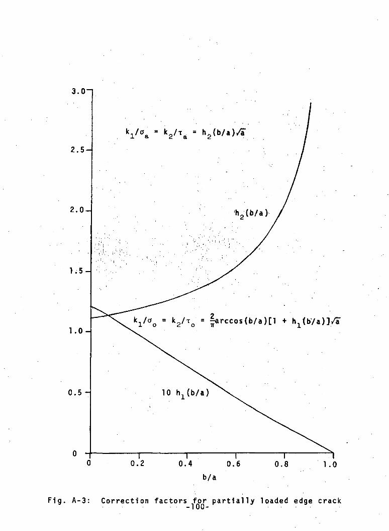
3.0-1

2.5-

2.0-

1.5-

1.0-

0.5 -

kl/Cfa = k2/Ta

ki/ao = k2/To = h1(b/a)]/i'

10 h1(b/a)

0.2 0.4 0.6 0.8 1.0

b/a

Fig. A-3: Correction factors for partially loaded edge crack

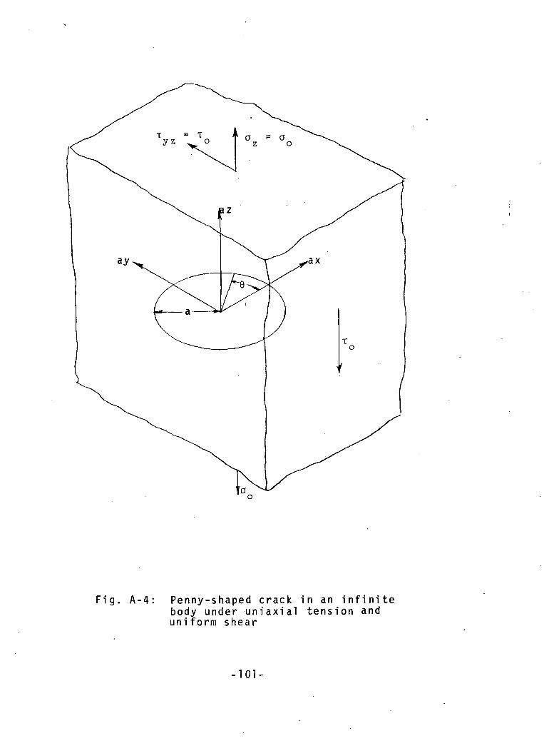
Fig. A-4: Penny-shaped crack in an infinitebody under uniaxial tension anduniform shear

-101-

Fig. A-5: Concentrated forces on a penny-shaped crack

-102-

uO>I/)I

CO«/> o>o cl-'f-OT3

c •<a ai

.«- <u

U Q.IX)

0 <1) ••o

-o c0> 3O.(O £

Ul 0)1 -Q

c. <ocCU4-o. o

-103-

Documents

ASE FILE COPY